Irreversible thermodynamics of thermoelectric devices:
From local framework to global description

Abstract

Thermoelectricity is traditionally explained via Onsager’s irreversible, flux-force framework. The coupled flows of heat and electric charge are modelled as steady-state flows, driven by the thermodynamic forces defined in terms of the gradients of local, intensive parameters like temperature and electrochemical potential. A thermoelectric generator is a device with a finite extension, and its performance is measured in terms of total power output and total entropy generation. These global quantities are naturally expressed in terms of discrete or global forces derived from their local counterparts. We analyze the thermodynamics of thermoelectricity in terms of global flux-force relations. These relations clearly show the additional quadratic dependence of the driver flux on global forces, corresponding to the process of Joule heating. We discuss the global kinetic coefficients defined by these flux-force relations and prove that the equality of the global cross-coefficients is derived from a similar property of the local coefficients. Finally, we clarify the differences between the global framework for thermoelectric energy conversion and the recently proposed minimally nonlinear irreversible thermodynamic model.

I Introduction

In many transport phenomena, interesting effects arise due to coupling between different thermodynamic forces present simultaneously in the system. Thermoelectricity provides a physically transparent picture of this coupling between flows of heat and electric charge, which gives rise to the well-known Seebeck, Peltier, and Thomson effects Onsager1931 ; Callen1948 ; Domenicali1954 ; Callenbook1985 ; DavidJou2008 . These interference phenomena can be successfully described within the linear flux-force formalism of Onsager Onsager1931 . The aforesaid linear relationship between fluxes and forces derives from the usually small magnitudes of the thermodynamic forces driving the system. The latter are expressed as gradients of the locally defined intensive parameters and this framework invokes the local-equilibrium hypothesis Callen1948 .

Although, the thermodynamic explanation of the above phenomena treats them as steady-state processes at the local level, actual devices have macroscopic extensions and so their performance needs to be analyzed by scaling up the local description. This leads to the study of global quantities like total power output and total entropy generation by the device. Due to the increasing worldwide demand for efficient and environment-friendly energy convertors, many works have pursued optimization of the material properties as well as power output/cooling power of thermoelectric devices Gordon1991 ; DiSalvo1999 ; RIFFAT2003 ; Shakouri2011 ; Benenti2011 ; snyder2011 ; Goupil2011 ; Apertet2012B ; Apertet2013A ; Ouerdane2013 ; Wohlman2014 ; BENENTI2017 ; Jasleen2019 ; Ding2019 . It is noteworthy that a local, linear-irreversible model gives rise to nonlinear (quadratic) dissipation terms in the flux equations at the global level CWelton . In thermoelectricity, Joule heating plays the role of this dissipation term. Thus, despite the apparent presence of nonlinearities in thermal flux equations, the locally linear character of the underlying framework for thermoelectricity has been emphasized CWelton ; Apertet2013B .

With the advent of finite-time thermodynamics, the flux-force framework for irreversible phenomena has been extended to macroscopic heat devices too Caplan1965 ; VandenBroeck2005 ; Iyyappan2020 , where the fluxes still are linear functions of the global or discrete forces. Further, the so-called minimally nonlinear irreversible thermodynamic (MNLIT) model Izumida2012 ; Izumida2015 proposes generalized heat flux equations by incorporating a nonlinear, phenomenological term at the global level, akin to the dissipation term in thermoelectric devices. This model may be adapted for both autonomous as well as cyclic heat devices operating in finite time Esposito2010 ; Izumida2013 .

In this paper, our focus is on the thermoelectric flux-force relations at the global level. As with the standard Onsager-Callen framework, consideration of the total rate of entropy generation as a bilinear form leads to the identification of global thermodynamic forces. We show how the scale-up from a local description naturally leads us to express the driven flux as a linear function of these global or discrete forces. In consequence, we will see that the driver flux additionally follows a nonlinear dependence on these forces, equivalent to the presence of a nonlinear dissipation term discussed above. We also define global kinetic coefficients from these flux relations. A hallmark of the underlying local framework is the equality of kinetic cross-coefficients based on principle of microscopic time reversibility Onsager1931b . We observe a similar property of the global kinetic coefficients, which can be traced to its local counterpart.

The plan of the paper is as follows. In Section II, Onsager-Callen framework for a thermoelectric generator is discussed. In Section III, we identify the discrete or global forms of forces and express the fluxes in terms of these forces. We also obtain expressions for the global kinetic coefficients and prove Onsager reciprocity at the global level. In Section IV, our approach is compared with the MNLIT model. Finally, we conclude in Section V.

II Thermoelectric generator

Consider the thermoelectric material to be a one-dimensional, homogeneous substance of length $l$ and cross-sectional area $A$, with given values of electrical resistivity $\rho$, thermal conductivity $\kappa$, and Seebeck coefficient $\alpha$. This is the so-called Constant Properties model Ioffe1957 . The two arms of the thermoelectric module are in series electrically, while they are parallel to each other thermally (see Fig. 1).

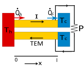
Figure 1: Schematic of thermoelectric heat engine. Two legs (yellow online) of a constant properties thermoelectric material (TEM) in simultaneous contact with a hot ($x=0$) and a cold ($x=l$) reservoir. Electric power, $P=\dot{Q}_{h}-\dot{Q}_{c}$, is drawn against an external load.

To describe thermoelectricity within linear-irreversible thermodynamic framework, the fluxes may be chosen as the particle current density $\vec{J}_{N}$ and the thermal current density $\vec{J}_{Q}$, locally driven by the respective affinities $-\vec{\nabla}\mu/T$ and $\vec{\nabla}(1/T)=-\vec{\nabla}T/T^{2}$, where $\mu$ and $T$ are the local electrochemical potential and the temperature, respectively. Assuming small magnitudes for such affinities, Onsager expressed the local fluxes as linear combination of these affinities:

$$\left(\begin{array}[]{c}\vec{J}_{N}\\ \vec{J}_{Q}\end{array}\right)=\left(\begin{array}[]{cc}L_{11}&L_{12}\\ L_{21}&L_{22}\end{array}\right)\left(\begin{array}[]{c}-{\vec{\nabla}\mu}/{T}\\ -\vec{\nabla}T/{T^{2}}\end{array}\right),$$ (1)

where the Onsager coefficients, $L_{ij}$, obey certain conditions Onsager1931 in order to satisfy the second law of thermodynamics. By defining the electric current density $\vec{J}=e\vec{J}_{N}$, and noting that $\vec{\nabla}\mu=e\vec{\nabla}V$, where $e$ is the charge on electron and $V$ is the electrostatic potential, we can write (1) as

$$\left(\begin{array}[]{c}\vec{J}\\ \vec{J}_{Q}\end{array}\right)=\left(\begin{array}[]{cc}e^{2}L_{11}&eL_{12}\\ eL_{21}&L_{22}\end{array}\right)\left(\begin{array}[]{c}-{\vec{\nabla}V}/{T}\\ -\vec{\nabla}T/{T^{2}}\end{array}\right).$$ (2)

It is known that the knowledge of Onsager coefficients $L_{ij}$ is equivalent to the knowledge of the quantities $\rho$, $\kappa$ and $\alpha$, whereby we have the following expressions Callen1948 :

$$L_{11} = \frac{T}{\rho e^{2}},$$

$$L_{12} = \frac{\alpha T^{2}}{\rho e}=L_{21},$$ (3)

$$L_{22} = T^{2}\left(\frac{\alpha^{2}T}{\rho}+\kappa\right).$$

Note that the cross-coefficients are equal by virtue of the principle of microscopic reversibility Onsager1931 . Secondly, even if the quantities $\rho$, $\kappa$, and $\alpha$ are assumed to be constant, the Onsager coefficients depend on local temperature $T$.

III From local to global affinities

Now, the Onsager-Callen framework was formulated for the steady-state description of irreversible phenomena in terms of forces and fluxes at the local level. In this section, we analyze how the flux-force relations are extended to the macroscopic level i.e. applied to the full length of the thermoelectric material.

The local rate of entropy production per unit volume, $\dot{s}$, is defined as the divergence of the entropy flux $\vec{J}_{s}=\vec{J}_{Q}/T$, so that $\dot{s}=\vec{\nabla}.(\vec{J}_{Q}/T)$, which can be written as the sum of products of fluxes and conjugate forces, as follows.

$$\dot{s}=\vec{J}.\left(\!-\frac{\vec{\nabla}V}{T}\!\right)+\vec{J}_{Q}(x).\vec{\nabla}\left(\!\frac{1}{T}\!\right),$$ (4)

where we have used Callen1948

$$\vec{\nabla}.\vec{J}_{Q}=-\vec{J}.\vec{\nabla}V.$$ (5)

Then, the rate of total entropy production per unit area (p.u.a) along the whole length of the material (1-d case) is $\dot{\cal S}=\int_{0}^{l}\dot{s}\;dx$, and given by

$$\dot{\cal S}=\frac{J_{Q}(l)}{T_{c}}-\frac{J_{Q}(0)}{T_{h}},$$ (6)

where $x=0(l)$ corresponds to the hot (cold) end of the material.

Now, the global power output p.u.a is given by

$${\cal P} = -\int_{0}^{l}\vec{\nabla}.\vec{J_{Q}}\;dx,$$ (7)

$$= J_{Q}(0)-J_{Q}(l).$$ (8)

Further, the use of Eq. (5) in (7), and the constant magnitude $|\vec{J}|\equiv J$ implies that

$${\cal P}=J(V_{c}-V_{h})\equiv J\Delta V.$$ (9)

From Eqs. (8) and (9), we can write Eq. (6) as

$$\dot{\cal S}=J\left(\!-\frac{\Delta V}{T_{c}}\!\right)+J_{Q}(0)\left(\!\frac{1}{T_{c}}-\frac{1}{T_{h}}\!\right).$$ (10)

Thus, the global rate of entropy production p.u.a is expressed in a bilinear form, $\dot{\cal S}\equiv{\cal J}_{1}X_{1}+{\cal J}_{2}X_{2}$, where the corresponding flux-force pairs are identified as follows.

$${\cal J}_{1} = J,\qquad\quad X_{1}=-\frac{\Delta V}{T_{c}},$$ (11)

$${\cal J}_{2} = J_{Q}(0),\quad X_{2}=\frac{1}{T_{c}}-\frac{1}{T_{h}}.$$ (12)

Comparing Eqs. (4) and (10), we observe how the pair of local affinities take up a discrete form, relevant for the global description. It is interesting to analyze this bilinear form further from irreversible thermodynamic point of view. For future comparison, we consider the rate of total entropy production, $\dot{S}=\dot{\cal S}A\equiv{J}_{1}X_{1}+{J}_{2}X_{2}$, where

$${J}_{1} = I,\qquad X_{1}=-\frac{\Delta V}{T_{c}},$$ (13)

$${J}_{2} = \dot{Q}_{h},\quad X_{2}=\frac{1}{T_{c}}-\frac{1}{T_{h}},$$ (14)

with $I=JA$ and $\dot{Q}_{h}=J_{Q}(0)A$.

III.1 Flux-force relations at the global level

Corresponding to linear flux-force relations at the local level, we now enquire into the relations between fluxes and forces at the macroscopic level. Note that the local flux-force relations are postulated to be linear within Onsager’s approach. Here, we wish to see how the fluxes, $J_{i}$, in Eqs. (13) and (14), are expressed in terms of the global or discrete affinities, $X_{i}$.

Firstly, from Eqs. (2) and (3), we can write

$$\vec{J}=-\frac{1}{\rho}\vec{\nabla}V-\frac{\alpha}{\rho}\vec{\nabla}T.$$ (15)

For the case of a 1-d thermoelectric element, we have

$$J=-\frac{1}{\rho}\frac{\partial V}{\partial x}-\frac{\alpha}{\rho}\frac{\partial T}{\partial x}.$$ (16)

Now, since the current density $J$ as well as $\rho$ and $\alpha$ are constant along the length of the material, integrating the above equation over $x\in[0,l]$, we obtain:

$$J.l=-\frac{\Delta V}{\rho}+\frac{\alpha}{\rho}\Delta T.$$ (17)

In the above, $\Delta V=V_{c}-V_{h}>0$, whereas $\Delta T=T_{h}-T_{c}>0$. Since $J=I/A$ and the resistance of the material is $R=\rho l/A$, we can write Eq. (17) as

$$I=-\frac{\Delta V}{R}+\frac{\alpha}{R}\Delta T.$$ (18)

which can be rewritten in the form

$$J_{1}=\frac{T_{c}}{R}X_{1}+\frac{\alpha T_{c}T_{h}}{R}X_{2},$$ (19)

following the definitions in Eqs. (13) and (14).

Thus, we note that the flux $J_{1}\equiv I$ is linear in the discrete forces $X_{1}$ and $X_{2}$.

Similarly, from Eqs. (2) and (3), the local thermal flux inside the thermoelectric material is given by:

$$J_{Q}(x)=-\frac{\alpha T(x)}{\rho}\frac{\partial V}{\partial x}-\left(\frac{\alpha^{2}T(x)}{\rho}+\kappa\right)\frac{\partial T}{\partial x},$$ (20)

which can be cast in the following form Apertet2013B :

$$J_{Q}(x)=\alpha T(x)J+\frac{\kappa\Delta T}{l}-\frac{\rho(l-2x)J^{2}}{2}.$$ (21)

Then, thermal currents at the end points of the thermoelectric material are evaluated to be

$$\dot{Q}_{h} = \alpha T_{h}I+K\Delta T-\frac{1}{2}RI^{2},$$ (22)

$$\dot{Q}_{c} = \alpha T_{c}I+K\Delta T+\frac{1}{2}RI^{2},$$ (23)

where $\dot{Q}_{c}=J_{Q}(l)A$. Also, $K=\kappa A/l$ is the thermal conductance. Then, the total power output of thermoelectric generator, $P=\dot{Q}_{h}-\dot{Q}_{c}$ is given by: $P=\alpha\Delta TI-RI^{2}$.

We close this subsection by expressing the thermal flux $J_{2}\equiv\dot{Q}_{h}$ in terms of the forces ($X_{1},X_{2}$). Substituting for $I=J_{1}$ from Eq. (19) into Eq. (22), we obtain

$$J_{2}=\frac{\alpha T_{c}T_{h}}{R}X_{1}+\left(\frac{\alpha^{2}T_{h}}{R}+K\right)T_{h}T_{c}X_{2}-\frac{T_{c}^{2}}{2R}X_{1}^{2}-\frac{\alpha^{2}T_{h}^{2}T_{c}^{2}}{2R}X_{2}^{2}-\frac{\alpha T_{h}T_{c}^{2}}{R}X_{1}X_{2}.$$ (24)

Thus, we have expressed the fluxes ($J_{1},J_{2}$) in terms of the global affinities ($X_{1},X_{2}$). Whereas $J_{1}$ is linear in the global forces, $J_{2}$ is explicitly non-linear in these forces. Alternately, nonlinearity lies in the quadratic dissipation term in Eq. (22), due to Joule heating Apertet2013B .

III.2 Global kinetic coefficients

We may formally define a set of kinetic coefficients by assuming expansion of the fluxes in terms of the global affinities, as follows. We write

$$J_{1} = {\cal L}_{11}X_{1}+{\cal L}_{12}X_{2},$$ (25)

$$J_{2} = {\cal L}_{21}X_{1}+{\cal L}_{22}X_{2}+{\cal O}[X_{j}^{2}].$$ (26)

Then, comparing Eq. (25) with (19), and Eq. (26) with (24), we obtain

$${\cal L}_{11} = \frac{T_{c}}{R},$$

$${\cal L}_{12} = \frac{\alpha T_{c}T_{h}}{R}={\cal L}_{21},$$ (27)

$${\cal L}_{22} = T_{c}T_{h}\left(\!\frac{\alpha^{2}T_{h}}{R}+K\!\right).$$

Additionally, we have higher-order coefficients related to the quadratic terms in Eq. (24). The above kinetic coefficients may be compared with their local counterparts in Eq. (3). Now, here also we observe the equality of the cross-coefficients. Recall, that the corresponding equality at the local level can be argued on the basis of microscopic time-reversibility. Interestingly, the equality at the macroscopic level can also be traced to the equality at the local level, as we show below.

From Eq. (2), we have

$$\vec{J}_{Q}(x)=\frac{L_{21}}{eL_{11}}\vec{J}-\frac{D}{L_{11}T^{2}}\vec{\nabla}T,$$ (28)

where $D=L_{11}L_{22}-L_{12}L_{21}$. If we do not invoke Eqs. (3), then, equivalent to Eq. (22), we can write

$$\dot{Q}_{h}=\frac{L^{{}^{\prime}}_{21}}{eL^{{}^{\prime}}_{11}}I+\frac{D^{\prime}A}{L^{{}^{\prime}}_{11}T^{2}_{h}l}\Delta T-\frac{T_{h}\;l}{2e^{2}L^{{}^{\prime}}_{11}A}I^{2},$$ (29)

where the primed Onsager coefficients are evaluated at $x=0$, or $T=T_{h}$. Alternately, in terms of the forces $X_{i}$, we can write $J_{2}\equiv\dot{Q}_{h}$ as

$$J_{2}=\frac{L^{{}^{\prime}}_{21}T_{c}}{eL^{{}^{\prime}}_{11}R}X_{1}+T_{c}T_{h}\left(\frac{D^{\prime}A}{L^{{}^{\prime}}_{11}T^{2}_{h}l}+\frac{\alpha L^{{}^{\prime}}_{21}T_{c}}{eL^{{}^{\prime}}_{11}R}\right)X_{2}+{\cal O}[X_{j}^{2}].$$ (30)

Comparing the above equation with Eq. (26), we identify ${\cal L}_{21}={L^{{}^{\prime}}_{21}T_{c}}/{eL^{{}^{\prime}}_{11}R}$, which turns out to be equal to ${\cal L}_{12}$, upon substituting from Eq. (3). Thus, we see that the equality ${\cal L}_{21}={\cal L}_{12}$ is consistent with the equality of Onsager coefficients ($L_{21}=L_{12}$) at the local level.

IV Comparison with MNLIT model

As mentioned in the Introduction, the so-called MNLIT model Izumida2012 assumes the following extended Onsager relations at the global level:

$$\bar{J}_{1} = \bar{\cal L}_{11}X_{1}+\bar{\cal L}_{12}X_{2},$$ (31)

$$\bar{J}_{2} = \bar{\cal L}_{21}X_{1}+\bar{\cal L}_{22}X_{2}-\gamma_{h}\bar{J}_{1}^{2},$$ (32)

where $\gamma_{h}>0$ specifies the strength of dissipation into the hot reservoir. The Onsager-like kinetic coefficients $\bar{\cal L}_{ij}$ are required to satisfy specific conditions in order to satisfy the second law at the global scale, $\dot{S}=\bar{J}_{1}X_{1}+\bar{J}_{2}X_{2}>0$.

Now, by inspection, one can notice that the thermoelectric generator at the global level of description, seems like a special case of the MNLIT model, with the kinetic coefficients $\bar{\cal L}_{ij}={\cal L}_{ij}$ as given by Eq. (27), and $\gamma_{h}=R/2$. However, important distinctions between the two frameworks need to be emphasized. First, in the thermoelectric case, the global flux-force relations are not postulated per se, but they emerge naturally when we scale up the description from a local to the global level, as shown in the previous sections. On the other hand, the flux-force relations in the form of Eqs. (31) and (32) are the premise of MNLIT model. Secondly, the reciprocity of cross-coefficients, $\bar{\cal L}_{21}=\bar{\cal L}_{12}$, is also something which is assumed in the MNLIT model. We have seen in the above that this feature is automatically satisfied for the thermoelectric model, and it is derived from the Onsager reciprocity at the local level. Thus, as has been emphasized earlier Apertet2013B ; Izumida2012 , the MNLIT model is not derived from some microscopic model, whereas the global description of thermoelectricity is derived from the underlying local linear-irreversible model. Still, the MNLIT model may be useful for a macroscopic modelling of irreversible thermal machines in the nonlinear regime Izumida2015 .

V Concluding remarks

In the above, we have analyzed the flux-force relations for a thermoelectric generator at global level, by scaling up from the local, linear-irreversible thermodynamic framework of Onsager and Callen. An important step is the identification of global affinities or thermodynamic forces and fluxes from the bilinear expression for the rate of total entropy generation. The flux-force relation is linear in case of the driven flux (electric current) while it is quadratic in the global forces for the driver flux (hot thermal flux). The nonlinear dissipation terms are known to be due to Joule heating. Further, these flux-force relations also yield expressions for the effective kinetic coefficients. We observe the equality of cross-coefficients and show that this is derived from the Onsager reciprocity at the local level. Although, the traditional picture of thermoelectricity is adequate to explain the global features of power generation and so on, we believe the global flux-force relations expressed in terms of discrete or global equivalent of the local forces, is also a valid depiction of the same phenomenon. Our analysis also clarifies the comparison with the other nonlinear phenomenological models such as MNLIT model. One can similarly formulate the global relations in the presence of magnetic field which breaks the time-reversal symmetry Apertet2013B . As may be expected, the global cross-coefficents are also not equal in this case. Finally, in the present paper, we have assumed ideal thermal contacts between the thermoelectric material and the reservoirs. In principle, one can also include the effect of finite-conductance heat exchangers in the performance analysis Gordon1991 . It will be interesting, albeit more involved, to investigate the global force-flux picture in the presence of internal as well as external irreversibilities.

Appendix A Choice of fluxes and affinities

We recall that the choice of fluxes and conjugate affinities is not unique within the Onsager framework Callen1948 . Thus, if the particle current density $\vec{J}_{N}$ and thermal current density $\vec{J}_{Q}$ are the fluxes of our description, then $-(\vec{\nabla}\mu)/T$ and $\vec{\nabla}(1/T)$, respectively, are the affinities. On the other hand, if $\vec{J}_{N}$ along with the energy current density, defined as: $\vec{J}_{E}(x)=\vec{J}_{Q}(x)+\mu(x)\vec{J}_{N}$, are chosen as the fluxes, then the corresponding affinities are, $-\vec{\nabla}(\mu/T)$ and $\vec{\nabla}(1/T)$, respectively. Analogously, the rate of entropy production at local level is given by:

$$\dot{s}=-\vec{J}_{N}.\vec{\nabla}\left(\frac{\mu}{T}\right)+\vec{J}_{E}(x).\vec{\nabla}\left(\frac{1}{T}\right),$$ (33)

The corresponding global rate of entropy production is then given by:

$$\dot{\cal S}=J_{N}\left(\frac{\mu_{h}}{T_{h}}-\frac{\mu_{c}}{T_{c}}\right)+J_{E}(0)\left(\frac{1}{T_{c}}-\frac{1}{T_{h}}\right),$$ (34)

which is in a bilinear form, expressed in terms of the corresponding fluxes and discrete forces.

Appendix B Thermoelectric refrigerator

In this section, we study the thermoelectric device working as a refrigerator. In this case, thermal and work flows invert their directions relative to the case of thermoelectric generator. At the local level, the fluxes are the electric flux density $\vec{J}$ and thermal flux density $\vec{J}_{Q}$, with conjugate affinities as $\vec{\nabla}V/T$ and $-\vec{\nabla}(1/T)=\vec{\nabla}T/T^{2}$. Local power input p.u.a. is given by $P=-\vec{\nabla}.\vec{J_{Q}}=\vec{J}.\vec{\nabla}V$. Now, the rate of local entropy production per unit volume, $\dot{s}=-\vec{\nabla}.(\vec{J}_{Q}/T)$ can be written as follows.

$$\dot{s}=\vec{J}.\left(\frac{\vec{\nabla}V}{T}\right)-\vec{J}_{Q}(x).\vec{\nabla}\left(\frac{1}{T}\right),$$ (35)

In this case, local force-flux relations are expressed as:

$$\left(\begin{array}[]{c}\vec{J}\\ \vec{J}_{Q}\end{array}\right)=\left(\begin{array}[]{cc}e^{2}L_{11}&eL_{12}\\ eL_{21}&L_{22}\end{array}\right)\left(\begin{array}[]{c}{\vec{\nabla}V}/{T}\\ \vec{\nabla}T/{T^{2}}\end{array}\right),$$ (36)

where the Onsager coefficients in terms of the properties of thermoelectric material have the same expressions as in Eq. (3).
Now, the rate of entropy production p.u.a along the 1-d thermoelectric material is given as

$$\dot{\cal S}=-\frac{J_{Q}(l)}{T_{c}}+\frac{J_{Q}(0)}{T_{h}},$$ (37)

which can be rewritten as

$$\dot{\cal S}=J\left(\frac{\Delta V}{T_{h}}\right)+J_{Q}(l)\left(\frac{1}{T_{h}}-\frac{1}{T_{c}}\right).$$ (38)

The rate of total entropy production, $\dot{S}=\dot{\cal S}A\equiv{J}_{1}X_{1}+{J}_{2}X_{2}$, where

$${J}_{1} = I,\qquad X_{1}=\frac{\Delta V}{T_{h}},$$ (39)

$${J}_{2} = \dot{Q}_{c},\quad X_{2}=\frac{1}{T_{h}}-\frac{1}{T_{c}}.$$ (40)

The above fluxes $J_{i}$ may be expressed in terms of macroscopic affinities $X_{i}$. By using Eqs. (3) and (36), we get

$$\vec{J}=\frac{\vec{\nabla}V}{\rho}+\alpha\frac{\vec{\nabla}T}{\rho}$$ (41)

Integrate it over the whole length, i.e, $x\in[0,l]$, we obtain $I={\Delta V}/{R}-\alpha{\Delta T}/{R}$, which can be written as

$$J_{1}=\frac{T_{h}}{R}X_{1}+\frac{\alpha T_{c}T_{h}}{R}X_{2}.$$ (42)

Also, thermal flux $J_{2}$ in terms of the global forces is given as

$$J_{2}=\frac{\alpha T_{h}T_{c}}{R}X_{1}+\left(\frac{\alpha^{2}T_{c}}{R}+K\right)T_{h}T_{c}X_{2}+{\cal O}[X_{j}^{2}]$$ (43)

It shows that $J_{2}$ is not a linear function of the global forces. Next, we compare Eqs. (42) and (43) with Eqs. (25) and (26) to get global kinetic coefficents:

$${\cal L}_{11} = \frac{T_{h}}{R},$$

$${\cal L}_{12} = \frac{\alpha T_{c}T_{h}}{R}={\cal L}_{21},$$ (44)

$${\cal L}_{22} = T_{c}T_{h}\left(\frac{\alpha^{2}T_{c}}{R}+K\right).$$

These coefficients of thermoelectric refrigerator may be compared with Eq. (27) for thermoelectric generator. We observe the difference in the form of diagonal coefficients. Further, it also shows that cross-coefficients preserve their equality which emerges from time-reversal symmetry at the microscopic level.

References

- (1) L. Onsager. Reciprocal relations in irreversible processes. ii. Phys. Rev., 38:2265–2279, Dec 1931.
- (2) H. B. Callen. The application of onsager’s reciprocal relations to thermoelectric, thermomagnetic, and galvanomagnetic effects. Phys. Rev., 73:1349–1358, Jun 1948.
- (3) C. A. Domenicali. Irreversible thermodynamics of thermoelectricity. Rev. Mod. Phys., 26:237–275, Apr 1954.
- (4) H. B Callen. Thermodynamics and an introduction to thermostatistics. New York : Wiley, 2nd ed edition, 1985. Rev. ed. of: Thermodynamics. 1960.
- (5) G. Lebon and D. Jou. Understanding non-equilibrium thermodynamics :. Springer,, Berlin, 2008.
- (6) J. M. Gordon. Generalized power versus efficiency characteristics of heat engines: The thermoelectric generator as an instructive illustration. American Journal of Physics, 59:551–555, June 1991.
- (7) F. J. DiSalvo. Thermoelectric cooling and power generation. Science, 285(5428):703–706, 1999.
- (8) S. B. Riffat and X. Ma. Thermoelectrics: a review of present and potential applications. Applied Thermal Engineering, 23(8):913 – 935, 2003.
- (9) A. Shakouri. Recent developments in semiconductor thermoelectric physics and materials. Annual Review of Materials Research, 41:399–431, 2011.
- (10) G. Benenti, K. Saito, and G. Casati. Thermodynamic bounds on efficiency for systems with broken time-reversal symmetry. Physical Review Letters, 106(23), 2011.
- (11) G. J. Snyder and E. S. Toberer. Complex thermoelectric materials. World Scientific, 2011.
- (12) C. Goupil, W. Seifert, K. Zabrocki, E. Müller, and G. J. Snyder. Thermodynamics of thermoelectric phenomena and applications. Entropy, 13(8):1481–1517, 2011.
- (13) Y. Apertet, H. Ouerdane, C. Goupil, and P. Lecoeur. Irreversibilities and efficiency at maximum power of heat engines: The illustrative case of a thermoelectric generator. Phys. Rev. E, 85(3):031116, March 2012.
- (14) Y. Apertet, H. Ouerdane, A. Michot, C. Goupil, and Ph. Lecoeur. On the efficiency at maximum cooling power. EPL (Europhysics Letters), 103(4):40001, 2013.
- (15) H. Ouerdane, C. Goupil, Y. Apertet, A. Michot, and A.l Abbout. A Linear Nonequilibrium Thermodynamics Approach to Optimization of Thermoelectric Devices, pages 323–351. Springer Berlin Heidelberg, Berlin, Heidelberg, 2013.
- (16) O. Entin-Wohlman, J.-H. Jiang, and Y. Imry. Efficiency and dissipation in a two-terminal thermoelectric junction, emphasizing small dissipation. Phys. Rev. E, 89:012123, Jan 2014.
- (17) G. Benenti, G. Casati, K. Saito, and R. S. Whitney. Fundamental aspects of steady-state conversion of heat to work at the nanoscale. Physics Reports, 694:1 – 124, 2017.
- (18) J. Kaur and R. S. Johal. Thermoelectric generator at optimal power with external and internal irreversibilities. Journal of Applied Physics, 126(12):125111, 2019.
- (19) Y. Ding, Y. Qiu, K. Cai, Q. Yao, S. Chen, L. Chen, and J. He. High performance n-type ag2se film on nylon membrane for flexible thermoelectric power generator. Nature Communications, 10(1):841, Feb 2019.
- (20) H. B. Callen and T. A. Welton. Irreversibility and generalized noise. Phys. Rev., 83:34–40, Jul 1951.
- (21) Y. Apertet, H. Ouerdane, C. Goupil, and P. Lecoeur. From local force-flux relationships to internal dissipations and their impact on heat engine performance: The illustrative case of a thermoelectric generator. Phys. Rev. E, 88(2):022137, August 2013.
- (22) O. Kedem and S. R. Caplan. Degree of coupling and its relation to efficiency of energy conversion. Trans. Faraday Soc., 61:1897–1911, 1965.
- (23) C. Van den Broeck. Thermodynamic efficiency at maximum power. Phys. Rev. Lett., 95:190602, Nov 2005.
- (24) I. Iyyappan and R. S. Johal. Efficiency of a two-stage heat engine at optimal power. EPL (Europhysics Letters), 128(5):50004, jan 2020.
- (25) Y. Izumida and K. Okuda. Efficiency at maximum power of minimally nonlinear irreversible heat engines. EPL (Europhysics Letters), 97(1):10004, jan 2012.
- (26) Y. Izumida, K. Okuda, J. M. M. Roco, and A. Calvo Hernández. Heat devices in nonlinear irreversible thermodynamics. Phys. Rev. E, 91:052140, May 2015.
- (27) M. Esposito, R. Kawai, K. Lindenberg, and C. Van den Broeck. Efficiency at maximum power of low-dissipation Carnot engines. Phys. Rev. Lett., 105:150603, Oct 2010.
- (28) Y. Izumida, K. Okuda, A. Calvo Hernández, and J. M. M. Roco. Coefficient of performance under optimized figure of merit in minimally nonlinear irreversible refrigerator. EPL (Europhysics Letters), 101(1):10005, jan 2013.
- (29) Lars Onsager. Reciprocal relations in irreversible processes. ii. Phys. Rev., 38:2265–2279, Dec 1931.
- (30) A. F. Ioffe. Semiconductor thermoelements, and Thermoelectric cooling. Infosearch, ltd., 1957.