Robust pricing and hedging via neural SDEs

Abstract.

Mathematical modelling is ubiquitous in the financial industry and drives key decision processes. Any given model provides only a crude approximation to reality and the risk of using an inadequate model is hard to detect and quantify. By contrast, modern data science techniques are opening the door to more robust and data-driven model selection mechanisms. However, most machine learning models are “black-boxes” as individual parameters do not have meaningful interpretation. The aim of this paper is to combine the above approaches achieving the best of both worlds. Combining neural networks with risk models based on classical stochastic differential equations (SDEs), we find robust bounds for prices of derivatives and the corresponding hedging strategies while incorporating relevant market data. The resulting model called neural SDE is an instantiation of generative models and is closely linked with the theory of causal optimal transport. Neural SDEs allow consistent calibration under both the risk-neutral and the real-world measures. Thus the model can be used to simulate market scenarios needed for assessing risk profiles and hedging strategies. We develop and analyse novel algorithms needed for efficient use of neural SDEs. We validate our approach with numerical experiments using both local and stochastic volatility models.

2010 AMS subject classifications: Primary: 65C30, 60H35; secondary: 60H30.

1. Introduction

1.1. Problem overview

Model uncertainty is an essential part of mathematical modelling but is particularly acute in mathematical finance and economics where one cannot base models on well established physical laws. Until recently, these models were mostly conceived in a three step fashion: 1) gathering statistical properties of the underlying time-series or the so called stylized facts; 2) handcrafting a parsimonious model, which would best capture the desired market characteristics without adding any needless complexity and 3) calibration and validation of the handcrafted model. Indeed, model complexity was undesirable, amongst other reasons, for increasing the computational effort required to perform in particular calibration but also pricing and risk calculations. With greater uptake of machine learning methods and greater computational power more complex models can now be used. This is due to the fact that arguably the most complicated and computationally expensive step of calibration has been addressed. Indeed, in the seminal paper [Hernandez, 2016] used neural networks to learn the calibration map from market data directly to model parameters. Subsequently, many papers followed [Liu et al., 2019, Ruf and Wang, 2019, Ruf and Wang, 2019, Benth et al., 2020, Gambara and Teichmann, 2020, Sardroudi, 2019, Horvath et al., 2019, Bayer et al., 2019, Bayer and Stemper, 2018, Vidales et al., 2018]. However, these approaches focused on the calibration of fixed parametric model, but did not address perhaps even the more important issue which is model selection and model uncertainty.

The approach taken in this paper is fundamentally different. We let the data dictate the model, while still keeping a strong prior on the model form. This is achieved by using SDEs for the model dynamics but instead of choosing a fixed parametrization for the model SDEs we allow the drift and diffusion to be given by an overparametrized neural networks. We will refer to these as Neural SDEs. These are shown to not only provide a systematic framework for model selection, but also, quite remarkably, to produce robust estimates on the derivative prices. Here, the calibration and model selection are done simultaneously. In this sense, model selection is data-driven. Since the neural SDE model is overparametrised, there is a large pool of possible models and the training algorithm selects a model. Unlike in handcrafted models, individual parameters do not carry any meaning. This makes it hard to argue why one model is better than another. Hence the ability to efficiently compute interval estimators, which algorithms in this paper provide, is critical.

In parallel to this work, a similar approach to modelling was taken in [Cuchiero et al., 2020], where the authors considered local stochastic volatility models with the leverage function approximated with a neural network. Their model can be seen as an example of a Neural SDEs.

Let us now consider a probability space $(\Omega,\mathcal{F},(\mathcal{F}_{t})_{t\in[0,T]},\mathbb{P})$ and a random variable $\Psi\in L^{2}(\mathcal{F}_{T})$ that represents the discounted payoff of a illiquid (path-dependent) derivative. The problem of calculating a market consistent price of a financial derivative can be seen as equivalent to finding a map that takes market data (e.g. prices of underlying assets, interest rates, prices of liquid options) and returns the no-arbitrage price of the derivative. Typically an Itô process $(X_{t}^{\theta})_{{t}\in[0,T]}$, with parameters $\theta\in\mathbb{R}^{p}$ has been the main component used in constructing such pricing function. Such parametric model induces a martingale probability measure, denoted by $\mathbb{Q}(\theta)$, which is then used to compute no-arbitrage price of derivatives. The market data (input data) here is represented by payoffs $\{\Phi_{i}\}_{i=1}^{M}$ of liquid derivatives, and their corresponding market prices $\{\mathfrak{p}(\Phi_{i})\}_{i=1}^{M}$. We will assume throughout that this price set is free of arbitrage. To make the model $\mathbb{Q}(\theta)$ consistent with market prices, one seeks parameters $\theta^{*}$ such that the difference between $\mathfrak{p}(\Phi_{i})$ and $\mathbb{E}^{\mathbb{Q}(\theta^{*})}[\Phi_{i}]$ is minimized for all $i=1,\ldots,M$ (w.r.t. some metric). If for all $i=1,\ldots,M$ we have $\mathfrak{p}(\Phi_{i})=\mathbb{E}^{\mathbb{Q}(\theta^{*})}[\Phi_{i}]$ then we will say the model is consistent with market data (perfectly calibrated). There may be infinitely many models that are consistent with the market. This is called Knightian uncertainty [Knight, 1971, Cohen et al., 2018].

Let $\mathcal{M}$ be the set of all martingale measures / models that are perfectly calibrated to market inputs. In the robust finance paradigm, see [Hobson, 1998, Cox and Obloj, 2011], one takes conservative approach and instead of computing a single price (that corresponds to a model from $\mathcal{M}$) one computes the price interval $(\inf_{\mathbb{Q}\in\mathcal{M}}\mathbb{E}^{\mathbb{Q}}[\Psi],\sup_{\mathbb{Q}\in\mathcal{M}}\mathbb{E}^{\mathbb{Q}}[\Psi])$. The bounds can be computed using tools from martingale optimal transport which also, through dual representation, yields corresponding super- and sub- hedging strategies, [Beiglböck et al., 2013]. Without imposing further constrains, the class of all calibrated models $\mathcal{M}$ might be too large and consequently the corresponding bounds too wide to be of practical use [Eckstein et al., 2019]. See however an effort to incorporate further market information to tighten the pricing interval, [Nadtochiy and Obloj, 2017, Aksamit et al., 2020]. Another shortcoming of working with the entire class of calibrated models $\mathcal{M}$ is that, in general, it is not clear how to obtain a practical/explicit model out of the measures that yields price bounds. For example, such explicit models are useful when one wants consistently calibrate under pricing measure $\mathbb{Q}$ and real-world measure $\mathbb{P}$ as needed for risk estimation and stress testing, [Broadie et al., 2011, Pelsser and Schweizer, 2016] or learn hedging strategies in the presence of transactional cost and an illiquidity constrains [Buehler et al., 2019].

1.2. Neural SDEs

Fix $T>0$ and for simplicity assume constant interest rate $r\in\mathbb{R}$. Consider parameter space $\Theta=\Theta^{b}\times\Theta^{\sigma}\subseteq\mathbb{R}^{p}$ and parametric functions $b:\mathbb{R}^{d}\times\Theta^{b}\rightarrow\mathbb{R}^{d}$ and $\sigma:\mathbb{R}^{d}\times\Theta^{\sigma}\rightarrow\mathbb{R}^{d\times n}$. Let $(W_{t})_{t\in[0,T]}$ be a $n$-dimensional Brownian motion supported on $(\Omega,\mathcal{F},(\mathcal{F}_{t})_{t\in[0,T]},\mathbb{Q})$ so that $\mathbb{Q}$ is the Wiener measure and $\Omega=C([0,T];\mathbb{R}^{n})$. We consider the following parametric SDE

(1.1) $$dX^{\theta}_{t}=b(t,X_{t}^{\theta},\theta)dt+\sigma(t,X_{t}^{\theta},\theta)dW_{t}\,.$$

We split $X^{\theta}$ which is the entire stochastic model into traded assets and non-tradable components. Let $X^{\theta}=(S^{\theta},V^{\theta})$, where $S$ are the traded assets and $V$ are the components that are not traded. We will assume that for all $t\in[0,T]$, $x=(s,v)\in\mathbb{R}^{d}$ and $\theta\in\mathbb{R}^{p}$ we will assume that

$$b(t,(s,v),\theta)=\big{(}rs,b^{V}(t,(s,v),\theta)\big{)}\in\mathbb{R}^{d}\,\,\,\text{and}\,\,\,\sigma(t,(s,v),\theta)=\big{(}\sigma^{S}(t,(s,v),\theta),\sigma^{V}(t,(s,v),\theta)\big{)}\,.$$

Then we can write (1.1) as

(1.2) $$\begin{split}dS^{\theta}_{t}&=rS_{t}^{\theta}\,dt+\sigma^{S}(t,X_{t}^{\theta},\theta)\,dW_{t}\,,\\ dV^{\theta}_{t}&=b^{V}(t,X_{t}^{\theta},\theta)\,dt+\sigma^{V}(t,X_{t}^{\theta},\theta)\,dW_{t}\,,\\ X^{\theta}_{t}&=(S^{\theta}_{t},V^{\theta}_{t})\,.\end{split}$$

Observe that $\sigma^{S}$ and $\sigma^{V}$ encode arbitrary correlation structures between the traded assets and the non-tradable components. Moreover, we immediately see that $(e^{-rt}S_{t})_{t\in[0,T]}$ is a (local) martingale and thus the model is free of arbitrage.

In a situation when $(b,\sigma)$ are defined to be neural networks (see Appendix C), we call the SDE (1.1) a neural SDE and we denote by $\mathcal{M}^{\text{nsde}}(\theta)$ the class of all solutions to (1.1). Note that due to universal approximation property of neural networks, see [Hornik, 1991, Sontag and Sussmann, 1997, Cuchiero et al., 2019], $\mathcal{M}^{\text{nsde}}(\theta)$ contains large class of SDEs solutions. Furthermore, neural networks can be efficiently trained with the stochastic gradient decent methods and hence one can easily seek calibrated models in $\mathcal{M}^{\text{nsde}}(\theta)$. Finally, neural SDE integrate black-box neural network type models with the known and well studied SDE models. One consequence of that is that one can: a) consistently calibrate these under the risk neutral measure as well as the real-world measure; b) easily integrate additional market information e.g constrains on realised variance; c) verify martingale property. We want to remark that for simplicity we work in Markovian setting, but one could consider neural-SDEs with path-dependent coefficients and/or consider more general noise processes. We postpone analysis of theses cases to follow up paper. By imposing suitable conditions on the coefficients $(b,\sigma)$ we know that unique solution to (1.1) exists, [Krylov, 1980, Chapter 2]. These conditions can be satisfied by neural networks e.g. by applying weight clipping. We denote the law of $X^{\theta}$ on $C([0,T];\mathbb{R}^{d})$ by $\mathbb{Q}(\theta):=\mathcal{L}((X_{t})_{t\in[0,T]})$.

Given a loss function $\ell:\mathbb{R}\times\mathbb{R}\rightarrow\mathbb{R}^{+}$, the search for calibrated model can be written as

$$\theta^{\ast}\in\arg\min_{\theta\in\Theta}\sum_{i=1}^{M}\ell(\mathbb{E}^{\mathbb{Q}(\theta)}[\Phi_{i}],\mathfrak{p}(\Phi_{i}))\,,\quad\text{where}\quad\mathbb{E}^{\mathbb{Q}(\theta)}[\Phi]=\int_{C([0,T],\mathbb{R}^{d})}\Phi(\omega)\mathcal{L}(X^{\theta})(d\omega)\,.$$

To extend the calibration consistently to the real world measure, assume that we are given some statistical facts (e.g. moments or other distributional properties) that the price process (or the non tradable components) should satisfy). Let $\zeta:[0,T]\times\mathbb{R}^{d}\times\mathbb{R}^{p}\to\mathbb{R}^{n}$ be another parametric function (e.g. neural network) and we extend the parameter space to $\Theta=\Theta^{b}\times\Theta^{\sigma}\times\Theta^{\zeta}\subseteq\mathbb{R}^{p}$. Let

$$\begin{split}b^{S,\mathbb{P}}(t,X^{\theta}_{t},\theta)&:=rS^{\theta}_{t}+\sigma^{S}(t,X^{\theta}_{t},\theta)\zeta(t,X^{\theta}_{t},\theta)\,,\\ b^{V,\mathbb{P}}(t,X^{\theta}_{t},\theta)&:=b^{V}(t,X^{\theta}_{t},\theta)+\sigma^{V}(t,X^{\theta}_{t},\theta)\zeta(t,X^{\theta}_{t},\theta)\,.\end{split}$$

We now define a real-world measure $\mathbb{P}(\theta)$ via the Radon–Nikodym derivative

$$\frac{d\mathbb{P}(\theta)}{d\mathbb{Q}(\theta)}:=\exp\left(\int_{0}^{T}\zeta(t,X^{\theta}_{t},\theta)\,dW_{t}+\frac{1}{2}\int_{0}^{T}|\zeta(t,X^{\theta}_{t},\theta)|^{2}\,dt\right)\,.$$

Under appropriate assumption on $\zeta$ (e.g. bounded) the measure $\mathbb{P}(\theta)$ is a probability measure and by using Girsanov theorem we can find Brownian motion $(W^{\mathbb{P}(\theta)}_{t})_{t\in[0,T]}$ such that

(1.3) $$\begin{split}dS^{\theta}_{t}&=b^{S,\mathbb{P}}(t,X^{\theta}_{t},\theta)\,dt+\sigma^{S}(t,X_{t}^{\theta},\theta)\,dW^{\mathbb{P}(\theta)}_{t}\,,\\ dV^{\theta}_{t}&=b^{V,\mathbb{P}}(t,X_{t}^{\theta},\theta)\,dt+\sigma^{V}(t,X_{t}^{\theta},\theta)\,dW^{\mathbb{P}(\theta)}_{t}\,.\end{split}$$

This is now the Neural SDE model in real-world measure $\mathbb{P}(\theta)$ and one would like use market data to seek $\zeta$. Let $\mathbb{P}^{\text{market}}$ denote empirical distribution of market data and $(\mathbb{E}^{\mathbb{P}^{\text{market}}}[\mathcal{S}_{i}])_{i=1}^{\tilde{M}}$ be a corresponding set statistics one aims to match. These might be autocorrelation function, realised variance or moments generating functions. The calibration to real-world measure, with $(b^{V},\sigma^{V},\sigma^{S})$ being fixed, consists of finding $\theta^{\ast}$ such that

$$\theta^{\ast}\in\arg\min_{\theta\in\Theta}\sum_{i=1}^{\tilde{M}}\ell(\mathbb{E}^{\mathbb{P}(\theta)}[\mathcal{S}_{i}],\mathbb{E}^{\mathbb{P}^{\text{market}}}[\mathcal{S}_{i}(\omega)])\,.$$

But in fact we can write

$$\mathbb{E}^{\mathbb{P}(\theta)}[\mathcal{S}_{i}]=\mathbb{E}^{\mathbb{Q}(\theta)}\bigg{[}\mathcal{S}_{i}\frac{d\mathbb{P}(\theta)}{d\mathbb{Q}(\theta)}\bigg{]}\,.$$

Thus we see that in this framework there needs to be no distinction between a derivative price $\Phi_{i}$ and a real-world statistic $\mathbb{E}^{\mathbb{P}^{\text{market}}}[\mathcal{S}_{i}]$. Hence from now on we will write only about risk-neutral calibrations bearing in mind that methodologically this leads to no loss of generality.

Let us connect neural SDEs to the concept of generative modelling, see  [Goodfellow et al., 2014, Kingma and Welling, 2013]. Let $\mathbb{Q}^{\text{market}}\in\mathcal{M}$ be the true martingale measure (so by definition all liquid derivatives are perfectly calibrated under this measure i.e. $\mathbb{E}^{\mathbb{Q}^{\text{market}}}[\Phi_{i}]=\mathfrak{p}(\Phi_{i})$ for all $i=1,\ldots,M$). We know that when (1.1) admits a strong solution then for any $\theta\in\mathbb{R}^{p}$ there exists a measurable map $G^{\theta}:\mathbb{R}^{d}\times C([0,T];\mathbb{R}^{n})\to C([0,T];\mathbb{R}^{d})$ such that $X^{\theta}=G^{\theta}(\zeta,W)$, see [Karatzas and Shreve, 2012, Corolarry 3.23]. Hence, one can view (1.1) as a generative model that maps $\mu$, the joint distribution of $X_{0}$ on $\mathbb{R}^{d}$ and the Wiener measure on $C([0,T];\mathbb{R}^{n})$ into $\mathbb{Q}^{\theta}=(G^{\theta}_{t})_{\#}\mu$. We see that by construction $G$ is a causal transport map i.e transport map that is adapted to filtration $(\mathcal{F}_{t})_{t\in[0,T]}$, see also [Acciaio et al., 2019, Lassalle, 2013].

One then seeks $\theta^{\ast}$ such that $G^{\theta^{\ast}}_{\#}\mu$ is a good approximation of $\mathbb{Q}^{\text{market}}$ with respect to user specified metric. In this paper we work with

$$D(G^{\theta}_{\#}\mu,\mathbb{Q}^{\text{market}}):=\sum_{i=1}^{M}\ell\left(\int_{C([0,T],\mathbb{R}^{d})}\Phi_{i}(\omega)(G^{\theta}_{\#}\mu)(d\omega),\int_{C([0,T],\mathbb{R}^{d})}\Phi_{i}(\omega)\mathbb{Q}^{\text{market}}(d\omega)\right)\,.$$

As we shall see in Sections 5.1 and 5.2 there are many Neural SDE models that can be calibrated well to market data and that produce significantly different prices for derivatives that were not part of the calibration data. In practice these would be illiquid derivatives where we require model to obtain prices. Therefore, we compute price intervals for illiquid derivatives within the class of calibrated neural SDEs models. To be more precise we compute

$$\inf_{\theta}\left\{\mathbb{E}^{\mathbb{Q}(\theta)}[\Psi]\,:\,D(G(\theta)_{\#}\mu_{0},\mathbb{Q}^{\text{market}})=0\right\}\,,\,\,\,\,\sup_{\theta}\left\{\mathbb{E}^{\mathbb{Q}(\theta)}[\Psi]\,:\,D(G(\theta)_{\#}\mu_{0},\mathbb{Q}^{\text{market}})=0\right\}\,.$$

We solve the above constraint optimisation problem by penalisation. See [Eckstein and Kupper, 2019] for related ideas.

1.3. Key conclusions and methodological contributions of this paper

The results in this paper presented below lead to the following conclusions.

1. Neural SDEs provide a systematic framework for model selection and produce robust estimates on the derivative prices. The calibration and model selection are done simultaneously and the thus the model selection is data-driven.

2. With neural SDEs, the modelling choices one makes are: networks architectures, structure of neural SDE (e.g. traded and non-traded assets), training methods and data. For classical handcrafted models the choice of the algorithm for calibrating parameters has not been considered as part of modelling choice, but for machine learning this is one of the key components. See Section 5, where we show how the change in initialisation of stochastic gradient method used for training leads to different prices of illiquid options, thus providing one way of obtaining price bounds. Furthermore even for basic local volalitly model that is unique for continuum of strikes and maturities, produces ranges of prices of illiquid derivatives when calibrated to finite data sets.

3. The above optimisation problem is not convex. Nonetheless, empirical experiments in Sections 5.1-5.2 demonstrate that the stochastic gradient decent methods used to minimise the loss functional $D$ converges to the set of parameters for which calibrated error is of order $10^{-5}$ to $10^{-4}$ for the square loss function. Theoretical framework for analysing such algorithms is being developed in [Šiška and Szpruch, 2020].

4. By augmenting classical risk models with modern machine learning approaches we are able to benefit from expressibility of neural networks while staying within realm of classical models, well understood by traders, risk managers and regulators. This mitigates, to some extent, the concerns that regulators have around use of black-box solutions to manage financial risk. Finally while our focus here is on SDE type models, the devised framework naturally extends to time-series type models.

The main methodological contributions of this work are as follows.

1. By leveraging martingale representation theorem we developed an efficient Monte Carlo based methods that simultaneously learns the model and the corresponding hedging strategy.

2. The calibration problem does not fit into classical framework of stochastic gradient algorithms, as the mini-batches of the gradient of the cost function are biased. We provide analysis of the bias and show how the inclusion of hedging strategies in training mitigates this bias.

3. We devise a novel, memory efficient randomised training procedure. The algorithm allows us to keep memory requirements constant, independently of the number of neural networks in neural SDEs. This is critical to efficiently calibrate to path dependent contingent claims. We provide theoretical analysis of our method in Section 4 and numerical experiment supporting the claims in Section 5.

The paper is organized as follows. In Section 2 we outline the exact optimization problem, introduce a deep neural network control variate (or hedging strategy), address the process of calibration to single/multiple option maturities and state the exact algorithms. In Section 3 we analyse the bias in Algorithms 1 and 2. In Section 4 we show that the novel, memory-efficient, drop-out-like training procedure for path-dependent derivatives does not introduce bias in the new estimator. Finally, the performance of Neural Local Volatility and Local Stochastic Volatility models is presented in Section 5. Some of the proofs and more detailed results from numerical experiments are relegated to the Appendix. The code used is available at github.com/msabvid/robust_nsde.

2. Robust pricing and hedging

Let $\ell:\mathbb{R}\times\mathbb{R}\to[0,\infty)$ be a convex loss function such that $\min_{x\in\mathbb{R},y\in\mathbb{R}}\ell(x,y)=0$. For example we can take $\ell(x,y)=|x-y|^{2}$. Given $\ell$, our aim is to solve the following optimisation problems:

1. Find model parameters $\theta^{*}$ such that model prices match market prices:

   (2.1) $$\theta^{\ast}\in\arg\min_{\theta\in\Theta}\sum_{i=1}^{M}\ell(\mathbb{E}^{\mathbb{Q}(\theta)}[\Phi_{i}],\mathfrak{p}(\Phi_{i}))\,.$$

   In practice this is equivalent to finding some $\theta^{*}$ such that $\sum_{i=1}^{M}\ell(\mathbb{E}^{\mathbb{Q}(\theta^{*})}[\Phi_{i}],\mathfrak{p}(\Phi_{i}))=0$. This is due to inherent overparametrization of Neural SDEs and the fact that $\ell\geq 0$ reaches minimum at zero.

2. Find model parameters $\theta^{l,*}$ and $\theta^{u,*}$ which provide robust arbitrage-free price bounds for an illiquid derivative, subject to available market data:

   (2.2) $$\begin{split}\theta^{l,\ast}&\in\arg\min_{\theta\in\Theta}\mathbb{E}^{\mathbb{Q}(\theta)}[\Psi]\,,\,\,\,\leavevmode\nobreak\ \text{ subject to}\,\,\,\sum_{i=1}^{M}\ell(\mathbb{E}^{\mathbb{Q}(\theta)}[\Phi_{i}],\mathfrak{p}(\Phi_{i}))=0\,\,,\\ \theta^{u,\ast}&\in\arg\max_{\theta\in\Theta}\mathbb{E}^{\mathbb{Q}(\theta)}[\Psi],\,\,\,\leavevmode\nobreak\ \text{ subject to}\,\,\,\sum_{i=1}^{M}\ell(\mathbb{E}^{\mathbb{Q}(\theta)}[\Phi_{i}],\mathfrak{p}(\Phi_{i}))=0\,.\end{split}$$

The no-arbitrage price of $\Psi$ over the class of neural SDEs used is then in $\Big{[}\mathbb{E}^{\mathbb{Q}(\theta^{l,*})},\mathbb{E}^{\mathbb{Q}(\theta^{u,*})}\Big{]}$.

2.1. Learning hedging strategy as a control variate

A starting point in the derivation of the practical algorithm is to estimate $\mathbb{E}^{\mathbb{Q}(\theta)}[\Phi]$ using a Monte Carlo estimator. Consider $(X^{i,\theta})_{i=1}^{N}$, a $N$ i.i.d copies of (1.1) and let $\mathbb{Q}^{N}(\theta):=\frac{1}{N}\sum_{i=1}^{N}\delta_{X^{i,\theta}}$ be empirical approximation of $\mathbb{Q}(\theta)$. Due to the Law of Large Numbers, $\mathbb{E}^{\mathbb{Q}^{N}(\theta)}[\Phi]$ converges to $\mathbb{E}^{\mathbb{Q}(\theta)}[\Phi]$ in probability. Moreover, the Central Limit Theorem tells us that

$$\mathbb{P}\left(\mathbb{E}^{\mathbb{Q}(\theta)}[\Phi]\in\left[\mathbb{E}^{\mathbb{Q}^{N}(\theta)}[\Phi]-z_{\alpha/2}\frac{\sigma}{\sqrt{N}},\mathbb{E}^{\mathbb{Q}^{N}(\theta)}[\Phi]+z_{\alpha/2}\frac{\sigma}{\sqrt{N}}\right]\right)\rightarrow 1\,\,\,\text{as}\,\,\,N\rightarrow\infty\leavevmode\nobreak\ ,$$

where $\sigma=\sqrt{\mathbb{V}\text{ar}[\Phi]}$ and $z_{\alpha/2}$ is such that $1-\text{CDF}_{Z}(z_{\alpha/2})=\alpha/2$ with $Z$ the standard normal distribution. We see that by increasing $N$, we reduce the width of the above confidence intervals, but this increases the overall computational cost. A better strategy is to find a good control variate i.e. we seek a random variable ${\Phi^{cv}}$ such that:

(2.3) $$\mathbb{E}^{\mathbb{Q}^{N}(\theta)}[\Phi^{cv}]=\mathbb{E}[\Phi]\quad\text{and}\quad\mathbb{V}\text{ar}[\Phi^{cv}]<\mathbb{V}\text{ar}[\Phi]\leavevmode\nobreak\ .$$

In the following we construct $\Phi^{cv}$ using hedging strategy. Similar approach has recently been developed in [Vidales et al., 2018] in the context of pricing and hedging with deep networks.

Martingale representation theorem (see for example Th. 14.5.1 in  [Cohen and Elliott, 2015]) provides a general methodology for finding Monte Carlo estimators with the above stated properties (2.3).

If $\Phi$ is such that $\mathbb{E}^{\mathbb{Q}}[|\Phi|^{2}]<\infty$, then there exists a unique process $Z=(Z_{t})_{t}$ adapted to the filtration $(\mathcal{F}_{t})_{t\in[0,T]}$ with $\mathbb{E}^{\mathbb{Q}}\left[\int_{t}^{T}|Z_{s}|^{2}\,ds\right]<\infty$ such that

$$\mathbb{E}[\Phi|\mathcal{F}_{0}]=\Phi-\int_{0}^{T}Z_{s}\,dW_{s}\,.$$

Define

$$\Phi^{cv}:=\Phi-\int_{0}^{T}Z_{s}\,dW_{s}\,,$$

and note that

$$\mathbb{E}^{\mathbb{Q}(\theta)}[\Phi^{cv}|\mathcal{F}_{0}]=\mathbb{E}^{\mathbb{Q}(\theta)}[\Phi|\mathcal{F}_{0}]\quad\text{and}\quad\mathbb{V}\text{ar}^{\mathbb{Q}(\theta)}[\Phi^{cv}|\mathcal{F}_{0}]=0\leavevmode\nobreak\ .$$

The process $Z$ has more explicit representations using corresponding (possibly path dependent) backward Kolomogorov equation or Bismut–Elworthy–Li formula. Both approaches require further approximation, see [Vidales et al., 2018] and [Vidales et al., 2020]. Here, this approximation will be provided by an additional neural network. Without loss of generality assume that $\Phi=\phi((X^{\theta}_{t})_{t\in[0,T]})$ for some $\phi:C([0,T],\mathbb{R}^{d})\rightarrow\mathbb{R}$. In the remaining of the paper, we will slightly abuse the notation to write $\Phi$ indistinctively as both the option and the mapping $C([0,T],\mathbb{R}^{d})\rightarrow\mathbb{R}$.

Consider now a neural network $\mathfrak{h}:[0,T]\times C([0,T],\mathbb{R}^{d})\times\mathbb{R}^{p}\rightarrow\mathbb{R}^{d}$ with parameters $\xi\in\mathbb{R}^{p^{\prime}}$ with $p^{\prime}\in\mathbb{N}$ and define the following learning task, in which $\theta$ (the parameters on the Neural SDE model) is fixed:

Find

(2.4) $$\xi^{\ast}\in\operatorname*{arg\,min}_{\xi}\mathbb{V}\text{ar}\left[\Phi((X^{\theta}_{t})_{t\in[0,T]})-\int_{0}^{T}\mathfrak{h}(s,(X^{\theta}_{s\wedge t})_{t\in[0,T]},\xi)dW_{s}\bigg{|}\mathcal{F}_{0}\right]\,.$$

In a similar manner one can derive $\Psi^{cv}$ for the payoff of the illiquid derivative for which we seek the robust price bounds. Then (2.2) can be restated as

(2.5) $$\begin{split}\theta^{l,\ast}&\in\arg\min_{\theta\in\Theta}\mathbb{E}^{\mathbb{Q}(\theta)}[\Psi^{cv}]\,,\,\,\,\leavevmode\nobreak\ \text{ subject to}\,\,\,\sum_{i=1}^{M}\ell(\mathbb{E}^{\mathbb{Q}(\theta)}[\Phi_{i}^{cv}],\mathfrak{p}(\Phi_{i}))=0\,,\\ \theta^{u,\ast}&\in\arg\max_{\theta\in\Theta}\mathbb{E}^{\mathbb{Q}(\theta)}[\Psi^{cv}]\,,\,\,\,\leavevmode\nobreak\ \text{ subject to}\,\,\,\sum_{i=1}^{M}\ell(\mathbb{E}^{\mathbb{Q}(\theta)}[\Phi_{i}^{cv}],\mathfrak{p}(\Phi_{i}))=0\,.\end{split}$$

The learning problem (2.5) is better than (2.2) from the point of view of algorithmic implementation, as it will enjoy lower Monte Carlo variance and hence will require simulation of fewer paths of the Neural SDE in each step of the stochastic gradient algorithm. Furthermore, when using (2.5) we learn a (possibly abstract) hedging strategy for trading in the underlying asset to replicate the derivative payoff. Since the market may be incomplete this abstract hedging strategy may not be usable in practice. More precisely, since the process $X^{\theta}$ will contain tradable as well as non-tradable assets, the control variate for the latter has to be adapted by either performing a projection or deriving a strategy for the corresponding tradable instrument.

To deduce a real hedging strategy recall that $X^{\theta}=(S^{\theta},V^{\theta})$ with $S^{\theta}$ being the tradable assets and $V^{\theta}$ the non-tradable components. Decompose the abstract hedging strategy as $\mathfrak{h}=(\mathfrak{h}^{S},\mathfrak{h}^{V})$. Let $\bar{S}^{\theta}_{t}:=e^{-rt}S^{\theta}_{t}$ and note that due to (1.2) we have

$$d(\bar{S}^{\theta}_{t})=e^{-rt}\sigma^{S}(t,X_{t}^{\theta},\theta)\,dW_{t}\,.$$

If we can solve $\mathfrak{h}^{S}=e^{-rt}\bar{\mathfrak{h}}^{S}_{t}\sigma^{S}(t,X^{\theta}_{t},\theta)$ for $\bar{\mathfrak{h}}^{S}_{t}$ then this is a real hedging strategy.

Therefore, an alternative approach to (2.4), possibly yielding a better hedge, but worse variance reduction would be to consider finding

(2.6) $$\bar{\xi}^{\ast}\in\operatorname*{arg\,min}_{\bar{\xi}}\mathbb{V}\text{ar}\left[\Phi((X_{t})_{t\in[0,T]})-\int_{0}^{T}\bar{\mathfrak{h}}(r,(X_{r\wedge t})_{t\in[0,T]},\bar{\xi})\,d\bar{S}^{\theta}_{r}\bigg{|}\mathcal{F}_{0}\right]$$

for some other neural network $\bar{\mathfrak{h}}$. This is the version we present in Algorithms 1 and 2.

2.2. Time discretization

In order to implement the (2.5) we define partition $\pi$ of $[0,T]$ as $\pi:=\{t_{0},t_{1},\ldots,t_{N_{\text{steps}}}=T\}$. We first approximate the stochastic integral in (2.4) with the appropriate Riemann sum. Depending on the choice of the neural network architecture approximating $\sigma$ in the Neural SDE (1.1) we may have $\sigma$ which grows super-linearly as a function of $x$. In such a case the moments of the classical Euler scheme are known blow up in the finite time, see [Hutzenthaler et al., 2011], even if moments of the solution to the SDE are finite. In order to avoid blow ups of moments of the simulated paths during training we apply tamed Euler method, see [Hutzenthaler et al., 2012, Szpruch and Zhāng, 2018]. The tamed Euler scheme is given by

(2.7) $$X_{t_{k+1}}^{\pi,\theta}=X_{t_{k}}^{\pi,\theta}+\frac{b(t_{k},X_{t_{k}}^{\pi,\theta},\theta)}{1+|b(t_{k},X_{t_{k}}^{\pi,\theta},\theta)|\sqrt{\Delta t_{k}}}\Delta t_{k}+\frac{\sigma(t_{k},X_{t_{k}}^{\pi,\theta},\theta)}{1+|\sigma(t_{k},X_{t_{k}}^{\pi,\theta},\theta)|\sqrt{\Delta t_{k}}}\Delta W_{t_{k+1}}\,,$$

with $\Delta t_{k}=t_{k+1}-t_{k}$ and $\Delta W_{t_{k+1}}=W_{t_{k+1}}-W_{t_{k}}$.

2.3. Algorithms

We now present the algorithm to calibrate the Neural SDE (1.1) to market prices of derivatives (Algorithm 1) and the algorithm to find robust price bounds for an illiquid derivative (Algorithm 2). Note that during training we aim to calibrate the SDE (1.1), and at the same time, adapt the abstract hedging strategy to minimise the variance (2.4). Therefore, we alternate two optimisations:

1. During each epoch, we optimise the parameters $\theta$ of the Neural SDE, while the parameters of the hedging strategy $\xi$ are fixed. In order to calculate the Monte Carlo estimator $\mathbb{E}^{\mathbb{Q}^{N}(\theta)}[\Phi^{cv}]$ we generate $N_{\text{trn}}$ paths $(x_{t_{n}}^{\pi,\theta,i})_{n=0}^{N_{\text{steps}}}:=(s_{t_{n}}^{\pi,\theta,i},v_{t_{n}}^{\pi,\theta,i})_{n=0}^{N_{\text{steps}}}$, $i=1,\ldots,N_{\text{trn}}$ using tamed Euler scheme on (1.1). Furthermore, we create a copy of the generated paths, denoting them $(\tilde{x}_{t_{n}}^{\pi,,i})_{n=0}^{N_{\text{steps}}}:=(\tilde{s}_{t_{n}}^{\pi,,i},\tilde{v}_{t_{n}}^{\pi,,i})_{n=0}^{N_{\text{steps}}}$ such that each $\tilde{x}_{t_{k}}^{\pi,,i}$ does not depend on $\theta$ anymore for the purposes of backward propagation when calculating the gradient. The paths $(\tilde{x}_{t_{n}}^{\pi,,i})_{n=0}^{N_{\text{steps}}}$ will be used as input to the parametrisation of the abstract hedging strategy $\mathfrak{h}$; as a result, in Algorithm 1 during this phase of the optimisation, the purpose of the hedging strategy is reducing the variance of $\mathbb{E}^{\mathbb{Q}^{N}(\theta)}[\Phi^{cv}]$ in order to speed up the convergence of the gradient descent algorithm.

2. During each epoch, we optimise the parameters $\xi$ of the parametrisation of the hedging strategy, while the parameters $\theta$ of the Neural SDE are fixed.

In both Algorithms 1 and 2 as well as in the numerical experiments, we use the squared error for the nested loss function: $\ell(x,y)=|x-y|^{2}$. Furthermore, the calibration of the Neural SDE to market derivative prices with robust price bounds for illiquid derivative in Algorithm 2 is done using a constrained optimisation using the method of Augmented Lagrangian [Hestenes, 1969], with the update rule of the Lagrange multipliers specified in Algorithm 3.

Algorithm 1 Calibration to market European option prices for one maturity

  Input: $\pi=\{t_{0},t_{1},\ldots,t_{N_{\text{steps}}}\}$ time grid for numerical scheme.

  Input: $(\Phi_{i})_{i=1}^{N_{\text{prices}}}$ option payoffs.

   Input: Market option prices $\mathfrak{p}(\Phi_{j})$, $j=1,\ldots,N_{\text{prices}}$.

  Initialisation: $\theta$ for neural SDE parameters, $N_{\text{trn}}\in\mathbb{N}$ large.

  Initialisation: $\xi$ for control variate approximation.

  for $\text{epoch}:1:N_{\text{epochs}}$ do

      Generate $N_{\text{trn}}$ paths $(x_{t_{n}}^{\pi,\theta,i})_{n=0}^{N_{\text{steps}}}:=(s_{t_{n}}^{\pi,\theta,i},v_{t_{n}}^{\pi,\theta,i})_{n=0}^{N_{\text{steps}}}$, $i=1,\ldots,N_{\text{trn}}$ using Euler scheme on (1.1). and create copies $(\tilde{x}_{t_{n}}^{\pi,i})_{n=0}^{N_{\text{steps}}}:=(\tilde{s}_{t_{n}}^{\pi,i},\tilde{v}_{t_{n}}^{\pi,i})_{n=0}^{N_{\text{steps}}}$ such that each $\tilde{x}_{t_{k}}^{\pi,i}$ does not depend on $\theta$ anymore, thus $\partial_{\theta}\tilde{x}_{t_{k}}^{\pi,i}=0$.

     During one epoch: Freeze $\xi$, use Adam (see  [Kingma and Ba, 2014]) to update $\theta$, where

$$\theta=\widehat{\operatorname*{arg\,min}_{\theta}}\sum_{j=1}^{N_{\text{prices}}}\left(\mathbb{E}^{N_{\text{trn}}}\left[\Phi_{j}\left(X^{\pi,\theta}\right)-\sum_{k=0}^{N_{\text{steps}}-1}\bar{\mathfrak{h}}(t_{k},\tilde{X}_{t_{k}}^{\pi,},\xi_{j})\Delta\tilde{\bar{S}}^{\pi,}_{t_{k}}\right]-\mathfrak{p}(\Phi_{j})\right)^{2}$$

and where $\mathbb{E}^{N_{\text{trn}}}$ denotes the empirical expected value calculated on the $N_{\text{trn}}$ paths.

     During one epoch: Freeze $\theta$, use Adam to update $\xi$, by optimising the sample variance

$$\xi=\widehat{\operatorname*{arg\,min}_{\xi}}\sum_{j=1}^{N_{\text{prices}}}\mathbb{V}\text{ar}^{N_{\text{trn}}}\left[\Phi_{j}\left(X^{\pi,\theta}\right)-\sum_{k=0}^{N_{\text{steps}}-1}\bar{\mathfrak{h}}(t_{k},X_{t_{k}}^{\pi,\theta},\xi_{j})\Delta\tilde{\bar{S}}^{\pi,\theta}_{t_{k}}\right]$$

  end for

  return  $\theta,\xi_{j}$ for all prices $(\Phi_{i})_{i=1}^{N_{\text{prices}}}$.

Algorithm 2 Calibration to vanilla prices for one maturity with lower bound for exotic price

  Input: $\pi=\{t_{0},t_{1},\ldots,t_{N_{\text{steps}}}\}$ time grid for numerical scheme.

  Input: $(\Phi_{i})_{i=1}^{N_{\text{prices}}}$ option payoffs.

   Input: Market option prices $\mathfrak{p}(\Phi_{j})$, $j=1,\ldots,N_{\text{prices}}$.

  Initialisation: $\theta$ for neural SDE parameters, $N_{\text{trn}}\in\mathbb{N}$ large.

  Initialisation: $\xi$ for control variate approximation.

  Initialisation: $\lambda,c$ for Augmented Lagrangian algorithm for constrained optimisation.

  for $\text{epoch}:1:N_{\text{epochs}}$ do

      Generate $N_{\text{trn}}$ paths $(x_{t_{n}}^{\pi,\theta,i})_{n=0}^{N_{\text{steps}}}:=(s_{t_{n}}^{\pi,\theta,i},v_{t_{n}}^{\pi,\theta,i})_{n=0}^{N_{\text{steps}}}$, $i=1,\ldots,N_{\text{trn}}$ using the Euler-type scheme on (1.1) and create copies $(\tilde{x}_{t_{n}}^{\pi,,i})_{n=0}^{N_{\text{steps}}}:=(\tilde{s}_{t_{n}}^{\pi,i},\tilde{v}_{t_{n}}^{\pi,i})_{n=0}^{N_{\text{steps}}}$ such that each $\tilde{x}_{t_{k}}^{\pi,i}$ does not depend on $\theta$ anymore, thus $\partial_{\theta}\tilde{x}_{t_{k}}^{\pi,i}=0$.

      During one epoch: Freeze $\xi$, use Adam to find $\theta^{N_{\text{trn}}}$, where

$$\begin{split}f(\theta)&:=\mathbb{E}^{N_{\text{trn}}}\left[\Psi(X^{\pi,\theta})-\sum_{k=0}^{N_{\text{steps}}-1}\bar{\mathfrak{h}}(t_{k},(\tilde{X}^{\pi,}_{t_{k}\wedge t_{j}})_{j=0}^{N_{\text{steps}}},\xi_{\Psi})\Delta\tilde{\bar{S}}^{\pi,}_{t_{k}}\right]\\ h(\theta)&:=\sum_{j=1}^{N_{\text{prices}}}\left(\mathbb{E}^{N_{\text{trn}}}\left[\Phi_{j}\left(X^{\pi,\theta}\right)-\sum_{k=0}^{N_{\text{steps}}-1}\bar{\mathfrak{h}}(t_{k},\tilde{X}_{t_{k}}^{\pi,},\xi_{j})\Delta\tilde{\bar{S}}^{\pi,}_{t_{k}}\right]-\mathfrak{p}(\Phi_{j})\right)^{2}\\ \theta&=\widehat{\operatorname*{arg\,min}_{\theta}}\,f(\theta)+\lambda h(\theta)+c\cdot(h(\theta))^{2}\end{split}$$

and where $\mathbb{E}^{N_{\text{trn}}}$ denotes the empirical expected value calculated on the $N_{\text{trn}}$ paths.

     During one epoch: Freeze $\theta$, use Adam to update $\xi$,

$$\begin{split}\xi&=\widehat{\operatorname*{arg\,min}_{\xi}}\sum_{j=0}^{N_{\text{prices}}}\mathbb{V}\text{ar}^{N_{\text{trn}}}\left[\Phi_{j}\left(X^{\pi,\theta}\right)-\sum_{k=0}^{N_{\text{steps}}-1}\bar{\mathfrak{h}}(t_{k},X_{t_{k}}^{\pi,\theta},\xi_{j})\Delta\tilde{\bar{S}}^{\pi,\theta}_{t_{k}}\right]+\\ &+\mathbb{V}\text{ar}^{N_{\text{trn}}}\left[\Psi\left(X^{\pi,\theta}\right)-\sum_{k=0}^{N_{\text{steps}}-1}\bar{\mathfrak{h}}(t_{k},(X_{t_{k}\wedge t_{j}}^{\pi,\theta})_{j=0}^{N_{\text{steps}}},\xi_{\Psi})\Delta\tilde{\bar{S}}^{\pi,\theta}_{t_{k}}\right]\end{split}$$

     Every 50 updates of $\theta$: Update $\lambda,c$ using Algorithm 3

  end for

  return  $\theta,\xi$.

Algorithm 3 Augmented Lagrangian parameters update

  Input: $\lambda>0,c>0$

  Input: $f(\theta)$ approximated exotic price with current values of $\theta$

  Input: $MSE(\theta)$ MSE of calibration to Vanilla prices with current values of $\theta$

  Update $\lambda:=\lambda+c\,MSE(\theta)$

  Update $c:=2c$

  return  $c$, $\lambda$

2.4. Algorithm for multiple maturities

Algorithms 1 and 2 calibrate the SDE (5.3) to one set of derivatives. If the derivatives for which we have liquid market prices can be grouped by maturity, as is the case e.g. for call / put prices, we can use a more efficient algorithm to achieve the calibration.

This follows the natural approach used e.g. in [Cuchiero et al., 2020], and in [Vidales et al., 2018] in the context of learning PDEs, where the networks for $b(t,X_{t}^{\theta},\theta)$ and $\sigma(t,X_{t}^{\theta},\theta)$ are split into different networks, one per maturity. Let $\theta=(\theta_{1},\ldots,\theta_{N_{m}})$, where $N_{m}$ is the number of maturities. Let

(2.8) $$\begin{split}b(t,X_{t}^{\theta},\theta)&:=\mathbf{1}_{t\in[T_{i-1},T_{i}]}(t)b^{i}(t,X_{t}^{\theta},\theta_{i}),\quad i\in\{1,\ldots,N_{m}\},\\ \sigma(t,X_{t}^{\theta},\theta)&:=\mathbf{1}_{t\in[T_{i-1},T_{i}]}(t)\sigma^{i}(t,X_{t}^{\theta},\theta_{i}),\quad i\in\{1,\ldots,N_{m}\},\end{split}$$

with each $b^{i}$ and $\sigma^{i}$ a feed forward neural network.

Regarding the SDE parametrisation, we fit feed-forward neural networks (see Appendix C) to the diffusion of the SDE of the price process under the risk-neutral measure. In the particular case, where we calibrate the Neural SDE to market data, without imposing any bounds on the resulting exotic option prices, one can then do an incremental learning as follows,

1. Consider the first maturity $T_{i}$ with $i=1$.

2. Calibrate the SDE using Algorithm 1 to the vanilla prices in maturity $T_{i}$.

3. Freeze the parameters of $\sigma_{i}$, set $i:=i+1$, and go back to previous step.

The above algorithm is memory efficient, as it only needs to backpropagate through that last maturity in each gradient descent step.

3. Analysis of the stochastic approximation algorithm for the calibration problem

3.1. Classical stochastic gradient

First, let us review the basics about stochastic gradient algorithm. Let $H:\Omega\times\Theta\rightarrow\mathbb{R}^{d}$. Consider the following optimisation problem

$$\min_{\theta\in\Theta}h(\theta)\,,\quad\text{where}\quad h(\theta):=\mathbb{E}[H(\theta)]\,.$$

Notice that the minimization task (2.1) does not fit this pattern as in our case the expectation is inside $\ell$.

Nevertheless we know that the classical gradient algorithm, with the learning rates $(\eta_{k})_{k=1}^{\infty}$, $\eta_{k}>0$ for all $k$, applied to this optimisation problem is given by

$$\theta_{k+1}=\theta_{k}-\eta_{k}\partial_{\theta}(\mathbb{E}[H(\theta_{k})])\,.$$

Under suitable conditions on $H$ and on $\eta_{k}$, it is known that $\theta_{k}$ converges to a minimiser of $h$, see [Benveniste et al., 2012]. As $\mathbb{E}[H(\theta_{k})]$ can rarely be computed explicitly, the above algorithm is not practical and is replaced with stochastic gradient descent (SGD) given by

$$\theta_{k+1}=\theta_{k}-\eta_{k}\frac{1}{N}\sum_{i=1}^{N}\partial_{\theta}H^{i}(\theta_{k})\,,$$

where $(H^{i}(\theta))_{i=1}^{N_{batch}}$ are independent samples from the distribution of $H(\theta)$ and $N\in\mathbb{N}$ is the size of the mini-batch. In particular $N$ could be one. The choice of a “good” estimator for $\mathbb{E}[H(\theta)]$ in the context of stochastic gradient algorithms is an active research area research, see e.g. [Majka et al., 2020]. When the estimator of $\mathbb{E}[H(\theta)]$ is unbiased, the SGD can be shown to converge to a minimum of $h$, [Benveniste et al., 2012].

3.2. Stochastic algorithm for the calibration problem

Recall that our overall objective in calibration is to minimize some $J=J(\theta)$ given by

$$J(\theta)=\sum_{i=1}^{M}\ell\Big{(}\mathbb{E}^{\mathbb{Q}(\theta)}[\Phi_{i}^{\text{cv}}],\mathfrak{p}(\Phi_{i})\Big{)}\,.$$

We write $X^{\theta}:=(X_{t}^{\theta})_{t\in[0,T]}$ and note that $\mathbb{E}^{\mathbb{Q}(\theta)}\big{[}\Phi_{i}\big{]}=\mathbb{E}\big{[}\Phi_{i}(X^{\theta})\big{]}$. Noting that in the calibration part of (2.1)–(2.5) the $\mathfrak{h}(s,(\tilde{X}_{s\wedge t})_{t\in[0,T]},\xi)d\tilde{\bar{S}}_{s}$ is fixed and hence $\mathbb{E}^{\mathbb{Q}}[\partial_{\theta}\Phi^{cv}_{i}(X^{\theta})]=\mathbb{E}^{\mathbb{Q}}[\partial_{\theta}\Phi_{i}(X^{\theta})]$

We differentiate $J=J(\theta)$ and work with the pathwise representation of this derivative (using language from [Glasserman, 2013]). For that we impose the following assumption.

Assumption 3.1.

We assume that payoffs $G:=(\Psi,\Phi)$, $G:C([0,T],\mathbb{R}^{d})\rightarrow\mathbb{R}$ are such that

$$\partial_{\theta}\mathbb{E}^{\mathbb{Q}}\left[G(X^{\theta})\right]=\mathbb{E}^{\mathbb{Q}}\left[\partial_{\theta}G(X^{\theta})\right]\,.$$

We refer reader to [Glasserman, 2013, chapter 7] for exact conditions when exchanging integration and differentiation is possible. We also remark that for the payoffs for which the Assumption 3.1 does not hold, one can use likelihood method and more generally Malliavin weights approach for computing greeks, [Fournié et al., 1999]. We don’t pursue this here for simplicity.

Writing $\ell=\ell(x,y)$, applying Assumption 3.1 and noting that $\mathbb{E}^{\mathbb{Q}(\theta)}\big{[}\Phi_{i}\big{]}=\mathbb{E}\big{[}\Phi(X^{\theta})\big{]}$ we see that

$$\begin{split}\partial_{\theta}J(\theta)&=\sum_{i=1}^{M}(\partial_{x}\ell)\Big{(}\mathbb{E}^{\mathbb{Q}(\theta)}[\Phi_{i}^{\text{cv}}],\mathfrak{p}(\Phi_{i})\Big{)}\partial_{\theta}\mathbb{E}^{\mathbb{Q}(\theta)}\big{[}\Phi_{i}^{\text{cv}}\big{]}\\ &=\sum_{i=1}^{M}(\partial_{x}\ell)\Big{(}\mathbb{E}[\Phi_{i}^{\text{cv}}(X^{\theta})],\mathfrak{p}(\Phi_{i})\Big{)}\mathbb{E}\big{[}\partial_{\theta}\Phi_{i}(X^{\theta})\big{]}\,.\end{split}$$

Hence, if we wish to update $\theta$ to some $\tilde{\theta}$ in such a way that $J$ is decreased then we need to take (for some $\gamma>0$)

$$\tilde{\theta}=\theta-\gamma\sum_{i=1}^{M}(\partial_{x}\ell)\Big{(}\mathbb{E}[\Phi_{i}^{\text{cv}}(X^{\theta})],\mathfrak{p}(\Phi_{i})\Big{)}\mathbb{E}\big{[}\partial_{\theta}\Phi_{i}(X^{\theta})\big{]}$$

so that

$$\begin{split}\frac{d}{d\varepsilon}J(\theta+\varepsilon(\tilde{\theta}-\theta))\Big{\rvert}_{\varepsilon=0}&=\sum_{i=1}^{M}(\partial_{x}\ell)\Big{(}\mathbb{E}[\Phi_{i}^{\text{cv}}(X^{\theta})],\mathfrak{p}(\Phi_{i})\Big{)}\mathbb{E}\big{[}\partial_{\theta}\Phi_{i}(X^{\theta})\big{]}(\tilde{\theta}-\theta)\\ &=-\gamma\bigg{|}\sum_{i=1}^{M}(\partial_{x}\ell)\Big{(}\mathbb{E}[\Phi_{i}^{\text{cv}}(X^{\theta})],\mathfrak{p}(\Phi_{i})\Big{)}\mathbb{E}\big{[}\partial_{\theta}\Phi_{i}(X^{\theta})\big{]}\bigg{|}^{2}\leq 0\,.\end{split}$$

If we had one network for each time step, leading to some resnet-like-network architecture for the time discretization then it may be more efficient to use a backward equation representation in the training. This representation can be derived using similar analysis as in [Jabir et al., 2019] (see also [Šiška and Szpruch, 2020]).

Since the summation plays effectively no role in further analysis we will assume, without loss of generality, that $M=1$ and work with the objective

$$h(\theta)=\ell\Big{(}\mathbb{E}^{\mathbb{Q}(\theta)}[\Phi^{\text{cv}}],\mathfrak{p}(\Phi)\Big{)}\,.$$

Then in the gradient step update we have

$$\partial_{\theta}h(\theta)=\partial_{x}\ell\left(\mathbb{E}^{\mathbb{Q}}[\Phi^{cv}(X^{\theta})],\mathfrak{p}(\Phi)\right)\mathbb{E}^{\mathbb{Q}}[\partial_{\theta}\Phi(X^{\theta})]\,,$$

Since $\ell$ is typically not an identity function, a mini-batch estimator of $\partial_{\theta}h(\theta)$, obtained by replacing $\mathbb{Q}$ with $\mathbb{Q}^{N}$ given by

$$\partial_{\theta}h^{N}(\theta):=\partial_{x}\ell\left(\mathbb{E}^{\mathbb{Q}^{N}}[\Phi^{cv}(X^{\theta})],\mathfrak{p}(\Phi)\right)\mathbb{E}^{\mathbb{Q}^{N}}[\partial_{\theta}\Phi(X^{\theta})]\,,$$

is a biased estimator of $\partial_{\theta}h$. Nonetheless the bias can be estimated in terms of number of samples $N$ and the variance. The fact the bias is controlled by the variance justifies why it is important to reduce the variance when calibrating the models with stochastic gradient algorithm. An alternative perspective is to view $\partial_{\theta}h^{N}(\theta)$ as non-linear function of $\mathbb{Q}^{N}$. It turns out that that there is a general theory studying smoothness and corresponding expansions of such functions of measures and we refer reader to [Chassagneux et al., 2019] for more details.

In Appendix A we provide a result on the bias for a general loss function. For the square loss function the bias is given below.

Theorem 3.2.

Let Assumption 3.1 hold. Consider the family of neural SDEs (1.1). For $\ell(x,y)=|x-y|^{2}$, we have

$$\begin{split}&\left|\mathbb{E}^{\mathbb{Q}}\left[\partial_{\theta}h^{N}(\theta)\right]-\partial_{\theta}h(\theta)\right|\leq\frac{2}{N}\left(\mathbb{V}ar^{\mathbb{Q}}[\Phi^{cv}(X^{\theta})]\right)^{1/2}\left(\mathbb{V}ar^{\mathbb{Q}}[\partial_{\theta}\Phi(X^{\theta})]\right)^{1/2}\,.\end{split}$$

Proof.

This is an immediate consequence of Theorem A.1. ∎

Hence, we see that by reducing the variance of the first term we are also reducing the bias of the gradient. This justifies superiority of learning task (2.5) over (2.2).

4. Analysis of the randomised training

4.1. Case of general cost function $\ell$

While the idea of calibrating to one maturity at the time described in Section 2.4 works well if our aim is only to calibrate to vanilla options, it cannot be directly applied to learn robust bounds for path dependent derivatives, see (2.2). This is because the payoff of path dependent derivatives, in general, is not an affine function of maturity. On the other hand training all neural networks at every maturity all at once, makes every step of the gradient algorithm used for training computationally heavy.

In what follows we introduce a randomisation of the gradient so that at each step of the gradient algorithm the derivatives with respect to the network parameters are computed at only one maturity at the time while keeping parameters at all other maturities unchanged. This is similar to the popular dropout method, see [Srivastava et al., 2014], that is known to help with overfitting when training deep neural networks but for us the main aim is computational efficiency. Recall how we split the networks for drift and diffusion

(2.8’) $$\begin{split}b(t,X_{t}^{\theta},\theta)&:=\mathbf{1}_{t\in[T_{i-1},T_{i}]}(t)b^{i}(t,X_{t}^{\theta},\theta_{i}),\quad i\in\{1,\ldots,N_{m}\},\\ \sigma(t,X_{t}^{\theta},\theta)&:=\mathbf{1}_{t\in[T_{i-1},T_{i}]}(t)\sigma^{i}(t,X_{t}^{\theta},\theta_{i}),\quad i\in\{1,\ldots,N_{m}\},\end{split}$$

Let $U\sim\mathbb{U}[1,\ldots,N_{m}]$ be a uniform random variable over set $[1,\dots,N_{m}]$ defined on a new probability space $(\Omega^{\mathbb{U}},\mathcal{F}^{\mathbb{U}},(\mathcal{F}^{\mathbb{U}}_{t})_{t\in[0,T]},\mathbb{P}^{\mathbb{U}})$. Let $Z$ be given by

$$\begin{split}dZ_{t}^{\theta}(U)=&\bigg{(}\sum_{i=1}^{N_{m}}\mathbf{1}_{[T_{i-1},T_{i}]}(t)\partial_{x}b^{i}(t,X_{t}^{\theta},\theta_{i})Z_{t}^{\theta}(U)+N\mathbf{1}_{[T_{U-1},T_{U}]}(t)\partial_{\theta_{U}}b^{U}(t,X_{t}^{\theta},\theta_{U})\bigg{)}\,dt\\ &+\bigg{(}\sum_{i=1}^{N_{m}}\mathbf{1}_{[T_{i-1},T_{i}]}(t)\partial_{x}\sigma^{i}(t,X_{t}^{\theta},\theta_{i})Z_{t}^{\theta}(U)+N\mathbf{1}_{[T_{U-1},T_{U}]}(t)\partial_{\theta_{U}}\sigma^{U}(t,X_{t}^{\theta},\theta_{U})\bigg{)}\,dW_{t}\,,\end{split}$$

where $b^{U},\sigma^{U}$ are simply neural networks sampled from the random index $U$.

Theorem 4.1.

Assume $\partial_{x}[b,\sigma](t,\cdot,\theta)$ exists and is bounded with $(t,\theta)$ fixed and $\partial_{\theta}[b,\sigma](t,x,\cdot)$ exists and is bounded with $(t,x)$ fixed. Let $h(\theta)=\ell(\mathbb{E}^{\mathbb{Q}(\theta)}[\phi(X_{t}^{\theta})],\mathfrak{p}(\Phi))$ and let its randomised gradient be

$$(\partial_{\theta}h)(\theta,U)=\partial_{x}\ell(\mathbb{E}^{\mathbb{Q}(\theta)}[\phi(X_{t}^{\theta})],\mathfrak{p}(\Phi))\,\mathbb{E}^{\mathbb{Q}(\theta)}[(\partial_{x}\phi)(X_{t}^{\theta})Z_{t}^{\theta}(U)]\,.$$

Then $\mathbb{E}^{\mathbb{U}}[(\partial_{\theta}h)(\theta,U)]=(\partial_{\theta}h)(\theta)$. In other words the randomised gradient is an unbiased estimator of $(\partial_{\theta}h)(\theta)$.

Less stringent assumption on derivatives of $b$ and $\sigma$ are possible, but we do not want to overburden the present article with technical details.

Proof.

It is well known, e.g [Krylov, 1999, Kunita, 1997], that

$$\begin{split}d(\partial_{\theta}X_{t}^{\theta})=\sum_{i=1}^{N_{m}}\mathbf{1}_{[T_{i-1},T_{i}]}(t)\bigg{[}&\Big{(}(\partial_{x}b^{i}(t,X_{t}^{\theta},\theta_{i})\partial_{\theta}X_{t}^{\theta}+\partial_{\theta_{i}}b^{i}(t,X_{t}^{\theta},\theta_{i})\Big{)}\,dt\\ &+\Big{(}(\partial_{x}\sigma^{i}(t,X_{t}^{\theta},\theta_{i})\partial_{\theta}X_{t}^{\theta}+\partial_{\theta_{i}}\sigma^{i}(t,X_{t}^{\theta},\theta_{i})\Big{)}\,dW_{t}\bigg{]}\,.\end{split}$$

Let $U\sim\mathbb{U}[1,\ldots,N_{m}]$ be a uniform random variable over set $[1,\dots,N_{m}]$ defined on a new probability space $(\Omega^{\mathbb{U}},\mathcal{F}^{\mathbb{U}},(\mathcal{F}^{\mathbb{U}}_{t})_{t\in[0,T]},\mathbb{P}^{\mathbb{U}})$. We introduce process $Z$ as follows

$$\begin{split}dZ_{t}^{\theta}(U)=&\bigg{(}\sum_{i=1}^{N_{m}}\mathbf{1}_{[T_{i-1},T_{i}]}(t)\partial_{x}b^{i}(t,X_{t}^{\theta},\theta_{i})Z_{t}^{\theta}(U)+N\mathbf{1}_{[T_{U-1},T_{U}]}(t)\partial_{\theta_{U}}b^{U}(t,X_{t}^{\theta},\theta_{U})\bigg{)}\,dt\\ &+\bigg{(}\sum_{i=1}^{N_{m}}\mathbf{1}_{[T_{i-1},T_{i}]}(t)\partial_{x}\sigma^{i}(t,X_{t}^{\theta},\theta_{i})Z_{t}^{\theta}(U)+N\mathbf{1}_{[T_{U-1},T_{U}]}(t)\partial_{\theta_{U}}\sigma^{U}(t,X_{t}^{\theta},\theta_{U})\bigg{)}\,dW_{t}\,.\end{split}$$

Note that

$$\mathbb{E}^{\mathbb{U}}[N\mathbf{1}_{[T_{U-1},T_{U}]}(t)\partial_{\theta_{U}}b^{U}(t,X_{t}^{\theta},\theta_{U})]=\sum_{i=1}^{N_{m}}\mathbf{1}_{[T_{i-1},T_{i}]}(t)\partial_{\theta_{i}}b^{i}(t,X_{t}^{\theta},\theta_{i})$$

and

$$\mathbb{E}^{\mathbb{U}}[N\mathbf{1}_{[T_{U-1},T_{U}]}(t)\partial_{\theta_{U}}\sigma^{U}(t,X_{t}^{\theta},\theta_{U})]=\sum_{i=1}^{N_{m}}\mathbf{1}_{[T_{i-1},T_{i}]}(t)\partial_{\theta_{i}}\sigma^{i}(t,X_{t}^{\theta},\theta_{i})\,.$$

Now using Fubini-type Theorem for Conditional Expectation, [Hammersley et al., 2019, Lemma A5], we have

$$\begin{split}d\mathbb{E}^{\mathbb{U}}\big{[}Z_{t}^{\theta}(U)\big{]}=&\bigg{(}\sum_{i=1}^{N_{m}}\mathbf{1}_{t\in[T_{i-1},T_{i}]}(t)\partial_{x}b^{i}(t,X_{t}^{\theta},\theta_{i})\mathbb{E}^{\mathbb{U}}\big{[}Z_{t}^{\theta}(U)\big{]}+\sum_{i=1}^{N_{m}}\mathbf{1}_{t\in[T_{i-1},T_{i}]}(t)\partial_{\theta_{i}}b^{i}(t,X_{t}^{\theta},\theta_{i})\bigg{)}\,dt\\ &+\bigg{(}\sum_{i=1}^{N_{m}}\mathbf{1}_{t\in[T_{i-1},T_{i}]}(t)\partial_{x}\sigma^{i}(t,X_{t}^{\theta},\theta_{i})E^{\mathbb{U}}\big{[}Z_{t}^{\theta}(U)\big{]}+\sum_{i=1}^{N_{m}}\mathbf{1}_{t\in[T_{i-1},T_{i}]}(t)\partial_{\theta_{i}}\sigma^{i}(t,X_{t}^{\theta},\theta_{i})\bigg{)}\,dW_{t}\,.\end{split}$$

Hence the process $\mathbb{E}^{\mathbb{U}}\big{[}Z_{t}^{\theta}(U)\big{]}$ solves the same linear equation as $\partial_{\theta}X^{\theta}$. As the equation has unique solution we conclude that

(4.1) $$\mathbb{E}^{\mathbb{U}}[Z_{t}^{\theta}(U)]=\partial_{\theta}X_{t}^{\theta}\,.$$

Recall that $h(\theta)=\ell(\mathbb{E}^{\mathbb{Q}(\theta)}[\phi(X_{t}^{\theta})],\mathfrak{p}(\Phi))$, and so

$$(\partial_{\theta}h)(\theta)=\partial_{x}\ell(\mathbb{E}^{\mathbb{Q}(\theta)}[\phi(X_{t}^{\theta})],\mathfrak{p}(\Phi))\,\mathbb{E}^{\mathbb{Q}(\theta)}[(\partial_{x}\phi)(X_{t}^{\theta})\partial_{\theta}X_{t}^{\theta}]\,.$$

Recall the randomised gradient

$$(\partial_{\theta}h)(\theta,U)=\partial_{x}\ell(\mathbb{E}^{\mathbb{Q}(\theta)}[\phi(X_{t}^{\theta})],\mathfrak{p}(\Phi))\,\mathbb{E}^{\mathbb{Q}(\theta)}[(\partial_{x}\phi)(X_{t}^{\theta})Z_{t}^{\theta}(U)]\,.$$

Note that due to (4.1)

$$\mathbb{E}^{\mathbb{U}}[\mathbb{E}^{\mathbb{Q}(\theta)}[(\partial_{x}\phi)(X_{t}^{\theta})Z_{t}^{\theta}(U)]]=\mathbb{E}^{\mathbb{Q}(\theta)}[(\partial_{x}\phi)(X_{t}^{\theta})\partial_{\theta}X_{t}^{\theta}]\,.$$

this implies that $\mathbb{E}^{\mathbb{U}}[(\partial_{\theta}h)(\theta,U)]=(\partial_{\theta}h)(\theta)$. ∎

4.2. Case of square loss function $\ell$

Here we show that, in the special case when $\ell(x,y)=|x-y|^{p}$, randomised gradient as described in Section 4 is an unbiased estimator of the full gradient even in the case when $\mathbb{Q}$ is replaced by its empirical measure $\mathbb{Q}^{N}$. Consequently standard theory on stochastic approximation applies. We base the presentation on the case $p=2$, as general case works in exact the same way. Let $(\bar{\Omega},\bar{\mathcal{F}},(\bar{\mathcal{F}_{t}})_{t\in[0,T]},\bar{\mathbb{P}})$ be a copy of $(\Omega,\mathcal{F},(\mathcal{F}_{t})_{t\in[0,T]},\mathbb{P})$. Then we write

$$h^{N}(\theta):=(\mathbb{E}^{\mathbb{Q}^{N}(\theta)}[\phi(X_{t}^{\theta})]-\mathfrak{p}(\Phi))^{2}=(\mathbb{E}^{{\bar{\mathbb{Q}}^{N}(\theta)}}[\phi(\bar{X}_{t}^{\theta})]-\mathfrak{p}(\Phi))(\mathbb{E}^{\mathbb{Q}^{N}(\theta)}[\phi(X_{t}^{\theta})]-\mathfrak{p}(\Phi_{i}))\,.$$

See also [Cuchiero et al., 2020] for the same observation. The gradient of $h$ is given by

$$\begin{split}(\partial_{\theta}h^{N})(\theta)=&(\mathbb{E}^{{\bar{\mathbb{Q}}^{N}(\theta)}}[\phi(\bar{X}_{t}^{\theta})]-\mathfrak{p}(\Phi))(\mathbb{E}^{\mathbb{Q}^{N}(\theta)}[(\partial_{x}\phi)(X_{t}^{\theta})\partial_{\theta}X_{t}^{\theta}]-\mathfrak{p}(\Phi_{i}))\\ &+(\mathbb{E}^{{\bar{\mathbb{Q}}^{N}(\theta)}}[(\partial_{x}\phi)(\bar{X}_{t}^{\theta})\partial_{\theta}\bar{X}_{t}^{\theta}]-\mathfrak{p}(\Phi))(\mathbb{E}^{\mathbb{Q}^{N}(\theta)}[\phi(X_{t}^{\theta})]-\mathfrak{p}(\Phi_{i}))\,.\end{split}$$

Equivalently

$$\begin{split}(\partial_{\theta}h^{N})(\theta)(\partial_{\theta}h^{N})(\theta)=&2(\mathbb{E}^{{\bar{\mathbb{Q}}^{N}(\theta)}}[\phi(\bar{X}_{t}^{\theta})]-\mathfrak{p}(\Phi))(\mathbb{E}^{\mathbb{Q}^{N}(\theta)}[(\partial_{x}\phi)(X_{t}^{\theta})\partial_{\theta}X_{t}^{\theta}]-\mathfrak{p}(\Phi_{i}))\\ =&2(\mathbb{E}^{{\bar{\mathbb{Q}}^{N}(\theta)}}[(\partial_{x}\phi)(\bar{X}_{t}^{\theta})\partial_{\theta}\bar{X}_{t}^{\theta}]-\mathfrak{p}(\Phi))(\mathbb{E}^{\mathbb{Q}^{N}(\theta)}[\phi(X_{t}^{\theta})]-\mathfrak{p}(\Phi_{i}))\,.\end{split}$$

To implement the above algorithm one simply needs to generate two independent sets of samples. Furthermore,

$$\begin{split}(\partial_{\theta}h^{N})(\theta,U)(\partial_{\theta}h^{N})(\theta)=&2(\mathbb{E}^{{\bar{\mathbb{Q}}^{N}(\theta)}}[\phi(\bar{X}_{t}^{\theta})]-\mathfrak{p}(\Phi))(\mathbb{E}^{\mathbb{Q}^{N}(\theta)}[(\partial_{x}\phi)(X_{t}^{\theta})Z_{t}^{\theta}(U)]-\mathfrak{p}(\Phi_{i}))\\ =&2(\mathbb{E}^{{\bar{\mathbb{Q}}^{N}(\theta)}}[(\partial_{x}\phi)(\bar{X}_{t}^{\theta})Z_{t}^{\theta}(U)]-\mathfrak{p}(\Phi))(\mathbb{E}^{\mathbb{Q}^{N}(\theta)}[\phi(X_{t}^{\theta})]-\mathfrak{p}(\Phi_{i}))\,.\end{split}$$

is an unbiased estimator of $(\partial_{\theta}h^{N})(\theta)$.

5. Testing neural SDE calibrations

All algorithms were implemented using PyTorch, see [Paszke et al., 2017] and [Paszke et al., 2019]. The code used is available at github.com/msabvid/robust_nsde. Our target data (European option prices for various strikes and maturities) is described in Appendix B. We assume that there is one traded asset $S=(S_{t})_{t\in[0,T]}$. We calibrate to European option prices

$$\mathfrak{p}(\Phi):=\mathbb{E}^{\mathbb{Q}(\theta)}[\Phi]=e^{-rT}\mathbb{E}^{\mathbb{Q}(\theta)}\left[\left(S_{T}-K\right)_{+}|\,S_{0}=1\right]$$

for maturities of $2,4,\ldots,12$ months and typically $21$ uniformly spaced strikes between in $[0.8,1.2]$. As an example of an illiquid derivative for which we wish to find robust bounds we take the lookback option

$$\mathfrak{p}(\Psi):=\mathbb{E}^{\mathbb{Q}(\theta)}[\Psi]=e^{-rT}\mathbb{E}^{\mathbb{Q}(\theta)}\left[\max_{t\in[0,T]}S_{t}-S_{T}|\,X_{0}=1\right]\,.$$

5.1. Local volatility neural SDE model

In this section we consider a Local Volatility (LV) Neural SDE model. It has been shown by [Dupire et al., 1994] (see also [Gyöngy, 1986]) that if the market data would consist of a continuum of call / put prices for all strikes and maturities then there is a unique function $\sigma$ such that with the price process

(5.1) $$dS_{t}=rS_{t}\,dt+S_{t}\,\sigma(t,S_{t})dW_{t}\,,\,\,\,S_{0}=1\,$$

the model prices and market prices match exactly. In practice only some calls / put prices are liquid in the market and so to apply [Dupire et al., 1994] one has to interpolate, in an arbitrage free way, the missing data. The choice of interpolation method is a further modelling choice on top of the one already made by postulating that the risky asset evolution is governed by (5.1).

We will use a Neural SDE instead of directly interpolating the missing data. Let our LV Neural SDE model be given by

(5.2) $$dS_{t}^{\theta}=rS_{t}^{\theta}dt+\sigma(t,S_{t}^{\theta},\theta)S_{t}^{\theta}dW_{t}^{\mathbb{Q}},\\$$

where $S_{t}^{\theta}\geq 0$, $S_{0}^{\theta}=1$ and $\sigma:[0,T]\times\mathbb{R}\times\mathbb{R}^{p}\to\mathbb{R}^{+}$ allows us to calibrate the model to observed market prices.

5.2. Local stochastic volatility neural SDE model

In this section we consider a Local Stochastic Volatility (LSV) Neural SDE model. See, for example, [Tian et al., 2015]. As in the Local Volatility Neural SDE model (5.2), we have the risky asset price price process $(S_{t})_{t\in[0,T]}$, where the drift is equal to the risk-free bond rate $r$. However, the volatility function in the LSV Neural SDE model now depends on $t$, $S_{t}$ and a stochastic process $(V_{t})_{t\in[0,T]}$. Here $(V_{t})_{t\in[0,T]}$ is not a traded asset. The model is then given by

(5.3) $$\begin{split}dS_{t}&=rS_{t}dt+\sigma^{S}(t,S_{t},V_{t},\nu)S_{t}\,dB^{S}_{t},\quad S_{0}=1,\\ dV_{t}&=b^{V}(V_{t},\phi)\,dt+\sigma^{V}(V_{t},\varphi)\,dB^{V}_{t},\quad V_{0}=v_{0},\\ d\langle B^{S},B^{V}\rangle_{t}&=\rho dt\end{split}$$

where $\theta:=\{\nu,\phi,\varphi,v_{0},\rho\},\,\,\rho,v_{0}\in\mathbb{R},$ as the set of (multi-dimensional) parameters that we aim to optimise so that the model is calibrated to the observed market data.

5.3. Deep learning setting for the LV and LSV neural SDE models

In the SDE (5.2) the function $\sigma$ and the SDE (5.3) the functions $\sigma^{S}$, $b^{V}$ and $\sigma^{V}$ are parametrised by one feed-forward neural network per maturity (see Section 2.4 and Appendix C) with $4$ hidden layers with $50$ neurons in each layer. The non-linear activation function used in each of the hidden layers is the linear rectifier relu. In addition, in $\sigma^{S}$ and $\sigma^{V}$ after the output layer we apply the non-linear rectifier softplus$(x)=\log(1+\exp(x))$ to ensure a positive output.

The parameterisation of the hedging strategy for the vanilla option prices is also a feed-forward linear network with 3 hidden layers, 20 neurons per hidden layer and relu activation functions. However, in order to get one hedging strategy per vanilla option considered in the market data, the output of $\mathfrak{h}(t_{k},s_{t_{k},\theta}^{i},\xi_{K_{j}})$ has as many neurons as strikes and maturities.

Finally, the parameterisation of the hedging strategy for the exotic options price is also a feed-forward network with 3 hidden layers, 20 neurons per hidden layer and relu activation functions.

The Neural SDEs (5.2) and (5.3) were discretized using the tamed Euler scheme (2.7) with $N_{\text{steps}}=8\times 12$ uniform time steps for $T=1$ year (i.e. $16$ for every $2$ months). The number of Monte Carlo trajectories in each stochastic gradient descent iteration was $N=4\times 10^{4}$ and the abstract hedging strategy was used as a control variate.

Finally in the evaluation of the calibrated Neural SDE, the option prices are calculated using $N=4\times 10^{5}$ trajectories of the calibrated Neural SDEs, which we generated with $2\times 10^{5}$ Brownian paths and their antithetic paths; in addition we also used the learned hedging strategies to calculate the Monte Carlo estimators with lower variance $\mathbb{E}^{\mathbb{Q}(\theta)}[\Phi_{i}^{cv}]$ and $\mathbb{E}^{\mathbb{Q}(\theta)}[\Psi^{cv}]$.

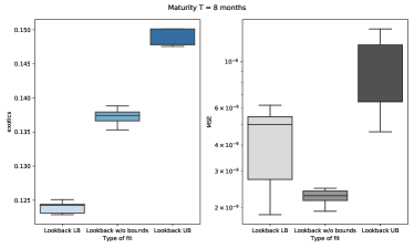
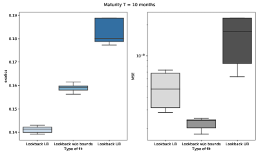
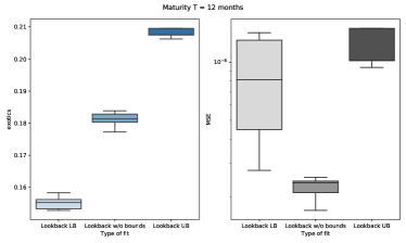
Figure 5.1. Box plots for the Local Volatility model (5.2). Exotic option price quantiles are in blue in the left-hand box-plot groups. The MSE quantiles of market data calibration is in grey, in the right-hand box-plot groups. Each box plot comes from 10 different runs of Neural SDE calibration. The three box-plots in each group arise respectively from aiming for a lower bound of the illiquid derivative(left), only calibrating to market and then pricing the illiquid derivative (middle) and aiming for a lower bound of the illiquid derivative (right).

5.4. Conclusions from calibrating for LV neural SDE

Each calibration is run $10$ times with different initialisations of the network parameters, with the goal to check the robustness of the exotic option price $\mathbb{E}^{\mathbb{Q}(\theta)}[\Psi]$ for each calibrated Neural SDE. The blue boxplots in Figure 5.1 provide different quantiles for the exotic option price $\mathbb{E}^{\mathbb{Q}(\theta)}[\Psi]$ and the obtained bounds after running We make the following observations from calibrating LV Neural SDE:

1. It is possible to obtain high accuracy of calibration with MSE of about $10^{-9}$ for $6$ month maturity, about $10^{-8}$ for 12 month maturity when the only target is to fit market data. If we are minimizing / maximizing the illiquid derivative price at the same time then the MSE increases somewhat so that it is about $10^{-8}$ for both $6$ and $12$ month maturities. See Figure 5.1. The calibration has been performed using $K=21$ strikes.

2. The calibration is accurate not only in MSE on prices but also on individual implied volatility curves, see Figure 5.2 and others in Appendix D.

3. As we increase the number of strikes per maturity the range of possible values for the illiquid derivative narrows. See Figure F.1 and Tables 1, 2, 3 and 4. The conjecture is that as the number of strikes (and maturities) would increase to infinity we would recover the unique $\sigma$ given by the Dupire formula that fits the continuum of European option prices.

4. With limited amount of market data (which is closer to practical applications) even the LV Neural SDE produces noticeable ranges for prices of illiquid derivatives, see again Figure 5.1.

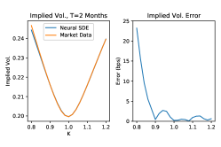
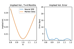
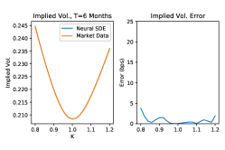
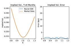
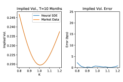
Figure 5.2. Calibrated neural SDE LV model and target market implied volatility comparison.

In Appendix F we provide more details on how different random seeds, different constrained optimization algorithms and different number of strikes used in the market data input affect the illiquid derivative price.

In Appendix D we present market price and implied volatility fit for constrained and unconstrained calibrations. High level of accuracy in all calibrations is achieved due to the hedging neural network incorporated into model training.

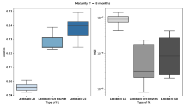
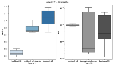
Figure 5.3. Box plots for the Local Stochastic Volatility model (5.3). Exotic option price quantiles are in blue in the left-hand box-plot groups. The MSE quantiles of market data calibration is in grey, in the right-hand box-plot groups. Each box plot comes from 10 different runs of Neural SDE calibration. The three box-plots in each group arise respectively from aiming for a lower bound of the illiquid derivative(left), only calibrating to market and then pricing the illiquid derivative (middle) and aiming for a lower bound of the illiquid derivative (right).

5.5. Conclusions from calibrating for LSV neural SDE

Each calibration is run ten times with different initialisations of the network parameters, with the goal to check the robustness of the exotic option price $\mathbb{E}^{\mathbb{Q}(\theta)}[\Psi]$ for each calibrated Neural SDE. The blue boxplots in Figure 5.3 provide different quantiles for the exotic option price $\mathbb{E}^{\mathbb{Q}(\theta)}[\Psi]$ and the obtained bounds after running all the experiments $10$ times. We make the following observations from calibrating LSV Neural SDE:

1. We note that our methods achieve high calibration accuracy to the market data (measured by MSE) with consistent bounds on the exotic option prices. See Figure 5.3.

2. The calibration is accurate not only in MSE on prices but also on individual implied volatility curves, see Figure 5.4 and others in Appendix E.

3. The LSV Neural SDE produces noticeable ranges for prices of illiquid derivatives, see again Figure 5.3.

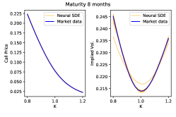
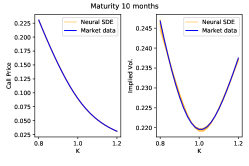
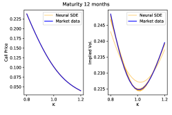
Figure 5.4. Comparing market and model data fit for the Neural SDE LSV model (5.3) when targeting only the market data. We see vanilla option prices and implied volatility curves of the 10 calibrated Neural SDEs vs. the market data for different maturities.

5.6. Hedging strategy evaluation

We calculate the error of the portfolio hedging strategy of the lookback option at maturity $T=6$ months, given by the empirical variance

$$\mathbb{V}ar^{N}\left[\psi\left(X^{\pi,\theta}\right)-\sum_{k=0}^{N_{\text{steps}}-1}\bar{\mathfrak{h}}(t_{k},(X_{t_{k}\wedge t_{j}}^{\pi,\theta})_{j=0}^{N_{\text{steps}}},\xi_{\Psi})\Delta\tilde{\bar{S}}^{\pi,\theta}_{t_{k}}\right]\,.$$

The histogram in Figure 5.5 is calculated on $N=400\,000$ different paths and provides the values of $s$,

$$s:=\Psi\left(X^{\pi,\theta}\right)-\sum_{k=0}^{N_{\text{steps}}-1}\bar{\mathfrak{h}}(t_{k},(X_{t_{k}\wedge t_{j}}^{\pi,\theta})_{j=0}^{N_{\text{steps}}},\xi_{\Psi})\Delta\tilde{\bar{S}}^{\pi,\theta}_{t_{k}}-\mathbb{E}^{N}\left[\Psi\left(X^{\pi,\theta}\right)\right]$$

i.e. such that

$$\mathbb{E}^{N}[s^{2}]=\mathbb{V}ar^{N}\left[\Psi\left(X^{\pi,\theta}\right)-\sum_{k=0}^{N_{\text{steps}}-1}\bar{\mathfrak{h}}(t_{k},(X_{t_{k}\wedge t_{j}}^{\pi,\theta})_{j=0}^{N_{\text{steps}}},\xi_{\Psi})\Delta\tilde{\bar{S}}^{\pi,\theta}_{t_{k}}\right].$$

We obtain $\mathbb{E}^{N}[s^{2}]=1.6\times 10^{-3}$.

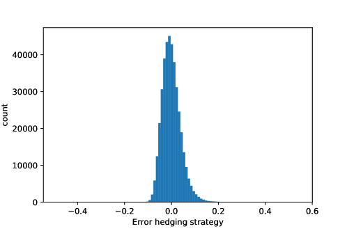
Figure 5.5. Error of the portfolio hedging strategy for the lookback option

Finally, we study the effect of the control variate parametrisation on the learning speed in Algorithm 1. Figure 5.6 displays the evolution of the Root Mean Squared Error of two runs of calibration to market vanilla option prices for two-months maturity: the blue line using Algorithm 1 with simultaneous learning of the hedging strategy, and the orange line without the hedging strategy. We recall that from Section 2.4, the Monte Carlo estimator $\partial_{\theta}h^{N}(\theta)$ is a biased estimator of $\partial_{\theta}h(\theta)$ An upper bound of the bias is given by Corollary 3.2, that shows that by reducing the variance of Monte Carlo estimator of the option price then the bias of $\partial_{\theta}h^{N}(\theta)$ is also reduced, yielding better convergence behaviour of the stochastic approximation algorithm. This can be observed in Figure 5.6.

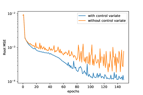
Figure 5.6. Root Mean Squared Error of calibration to Vanilla option prices with and without hedging strategy parametrisation

Declarations of Interest

The authors report no conflicts of interest. The authors alone are responsible for the content and writing of the paper.

Appendix A Bound on bias in gradient descent

We complete the analysis from Section 3.2 for a general loss function here.

Theorem A.1.

Let Assumption 3.1 hold. Consider the family of neural SDEs (1.1). We have

(A.1) $$\begin{split}|\mathbb{E}[\partial_{\theta}h^{N}(\theta)]-\partial_{\theta}h(\theta)|\leq&\left(\mathbb{E}\left[(\partial_{x}\ell(\mathbb{E}^{\mathbb{Q}^{N}(\theta)}[\Phi^{cv}(X^{\theta})],\mathfrak{p}(\Phi))-\partial_{x}\ell(\mathbb{E}^{\mathbb{Q}}[\Phi^{cv}(X^{\theta})],\mathfrak{p}(\Phi)))^{2}\right]\right)^{1/2}\\ &\times\left(\mathbb{E}\left[\left(\mathbb{E}^{\mathbb{Q}^{N}(\theta)}[\partial_{\theta}\Phi(X^{\theta})]\right)^{2}\right]\right)^{1/2}\,.\end{split}$$

If in addition we assume that the loss function $\ell$ is three times differentiable in the first variable with all its derivatives bounded, then

(A.2) $$\begin{split}&\left|\mathbb{E}^{\mathbb{Q}}\left[\partial_{\theta}h^{N}(\theta)\right]-\partial_{\theta}h(\theta)\right|\\ &\leq\frac{1}{2}\Big{\{}\|\partial_{x}^{3}\ell\|_{\infty}|\mathbb{E}^{\mathbb{Q}}[\partial_{\theta}\Phi(X^{\theta})]|\frac{1}{N}\mathbb{V}ar^{\mathbb{Q}}[\Phi^{cv}(X^{\theta})]\\ &+\|\partial_{x}^{3}\ell\|_{\infty}\left(\frac{1}{N}\mathbb{V}ar^{\mathbb{Q}}[\partial_{\theta}\Phi(X^{\theta})]\right)^{1/2}\left(\frac{1}{N^{3}}\mathbb{E}[(\Phi^{cv}(X^{\theta})-\mathbb{E}^{\mathbb{Q}}[\Phi^{cv}(X^{\theta})])^{4}]+\frac{3}{N^{2}}(\mathbb{V}ar^{\mathbb{Q}}[\Phi^{cv}(X^{\theta})])^{2}\right)^{1/2}\\ &+2\|\partial_{x}^{2}\ell\|_{\infty}\left(\frac{1}{N}\mathbb{V}ar^{\mathbb{Q}}[\partial_{\theta}\Phi(X^{\theta})]\right)^{1/2}\left(\frac{1}{N}\mathbb{V}ar^{\mathbb{Q}}[\Phi^{cv}(X^{\theta})]\right)^{1/2}\Big{\}}\,.\end{split}$$

Proof.

Observe that

$$\mathbb{E}\left[\mathbb{E}^{\mathbb{Q}^{N}}[\Phi^{cv}(X^{\theta})]\right]=\mathbb{E}^{\mathbb{Q}}[\Phi^{cv}(X^{\theta})]\quad\text{and}\quad\mathbb{E}\left[\mathbb{E}^{\mathbb{Q}^{N}}[\partial_{\theta}\Phi(X^{\theta})]\right]=\mathbb{E}^{\mathbb{Q}}[\partial_{\theta}\phi(X^{\theta})]\,.$$

Next, by adding and subtracting $\partial_{x}\ell(\mathbb{E}^{\mathbb{Q}}[\Phi^{cv}(X^{\theta})],\mathfrak{p}(\Phi))$ and using the Cauchy–Schwarz inequality we have

$$\begin{split}&|\mathbb{E}[\partial_{\theta}h^{N}(\theta)]-\partial_{\theta}h(\theta)|\\ &=\left|\mathbb{E}\left[\left(\partial_{x}\ell\left(\mathbb{E}^{\mathbb{Q}^{N}}[\Phi^{cv}(X^{\theta})],\mathfrak{p}(\Phi)\right)\pm\partial_{x}\ell\left(\mathbb{E}^{\mathbb{Q}}[\Phi^{cv}(X^{\theta})],\mathfrak{p}(\Phi)\right)\right)\mathbb{E}^{\mathbb{Q}^{N}}\left[\partial_{\theta}\Phi(X^{\theta})\right]\right]-\partial_{\theta}h(\theta)\right|\,.\\ \end{split}$$

Hence

$$\begin{split}&|\mathbb{E}[\partial_{\theta}h^{N}(\theta)]-\partial_{\theta}h(\theta)|\\ &=\left|\mathbb{E}\left[\left(\partial_{x}\ell\left(\mathbb{E}^{\mathbb{Q}^{N}}[\Phi^{cv}(X^{\theta})],\mathfrak{p}(\Phi)\right)-\partial_{x}\ell\left(\mathbb{E}^{\mathbb{Q}}[\Phi^{cv}(X^{\theta})],\mathfrak{p}(\Phi)\right)\right)\mathbb{E}^{\mathbb{Q}^{N}}\left[\partial_{\theta}\Phi(X^{\theta})\right]\right]\right|\\ &\leq\left(\mathbb{E}\left[\left(\partial_{x}\ell\left(\mathbb{E}^{\mathbb{Q}^{N}}[\Phi^{cv}(X^{\theta})],\mathfrak{p}(\Phi)\right)-\partial_{x}\ell\left(\mathbb{E}^{\mathbb{Q}}[\Phi^{cv}(X^{\theta})],\mathfrak{p}(\Phi)\right)\right)^{2}\right]\right)^{1/2}\left(\mathbb{E}\left[\mathbb{E}^{\mathbb{Q}^{N}}[\partial_{\theta}\Phi(X^{\theta})]\right]^{2}\right)^{1/2}\,.\end{split}$$

This concludes the proof of (A.1). To prove (A.2), we view $\partial_{\theta}h^{N}(\theta)$ as function of $(\mathbb{E}^{\mathbb{Q}^{N}}[\Phi^{cv}(X^{\theta})],\allowbreak\mathbb{E}^{\mathbb{Q}^{N}}[\partial_{\theta}\Phi(X^{\theta})])$ and expand into its Taylor series around $(\mathbb{E}^{\mathbb{Q}}[\Phi^{cv}(X^{\theta})],\mathbb{E}^{\mathbb{Q}}[\partial_{\theta}\Phi(X^{\theta})])$, i.e

$$\begin{split}&\partial_{\theta}h^{N}(\theta)=\partial_{\theta}h(\theta)\\ &+\partial_{x}^{2}\ell\left(\mathbb{E}^{\mathbb{Q}}[\Phi^{cv}(X^{\theta})],\mathfrak{p}(\Phi)\right)\mathbb{E}^{\mathbb{Q}}[\partial_{\theta}\Phi(X^{\theta})]\left(\mathbb{E}^{\mathbb{Q}^{N}}[\Phi^{cv}(X^{\theta})]-\mathbb{E}^{\mathbb{Q}}[\Phi^{cv}(X^{\theta})]\right)\\ &+\partial_{x}\ell\left(\mathbb{E}^{\mathbb{Q}}[\Phi^{cv}(X^{\theta})],\mathfrak{p}(\Phi)\right)\left(\mathbb{E}^{\mathbb{Q}^{N}}[\partial_{\theta}\Phi(X^{\theta})]-\mathbb{E}^{\mathbb{Q}}[\partial_{\theta}\Phi(X^{\theta})]\right)\\ &+\frac{1}{2}\int_{0}^{1}\Big{\{}\partial_{x}^{3}\ell\left(\xi_{1}^{\alpha},\mathfrak{p}(\Phi)\right)\xi_{2}^{\alpha}\left(\mathbb{E}^{\mathbb{Q}^{N}}[\Phi^{cv}(X^{\theta})]-\mathbb{E}^{\mathbb{Q}}[\Phi^{cv}(X^{\theta})]\right)^{2}\\ &\qquad+2\partial_{x}^{2}\ell\left(\xi_{1}^{\alpha},\mathfrak{p}(\Phi)\right)\left(\mathbb{E}^{\mathbb{Q}^{N}}[\partial_{\theta}\Phi(X^{\theta})]-\mathbb{E}^{\mathbb{Q}}[\partial_{\theta}\Phi(X^{\theta})]\right)\left(\mathbb{E}^{\mathbb{Q}^{N}}[\Phi^{cv}(X^{\theta})]-\mathbb{E}^{\mathbb{Q}}[\Phi^{cv}(X^{\theta})]\right)\Big{\}}d\alpha\,,\end{split}$$

where

$$\begin{split}\xi_{1}^{\alpha}=&\mathbb{E}^{\mathbb{Q}}[\Phi^{cv}(X^{\theta})]+\alpha\left(\mathbb{E}^{\mathbb{Q}^{N}}[\Phi^{cv}(X^{\theta})]-\mathbb{E}^{\mathbb{Q}}[\Phi^{cv}(X^{\theta})]\right)\,,\\ \xi_{2}^{\alpha}=&\mathbb{E}^{\mathbb{Q}}[\partial_{\theta}\Phi(X^{\theta})]+\alpha\left(\mathbb{E}^{\mathbb{Q}^{N}}[\partial_{\theta}\Phi(X^{\theta})]-\mathbb{E}^{\mathbb{Q}}[\partial_{\theta}\Phi(X^{\theta})]\right)\,.\end{split}$$

Hence, using Cauchy-Schwarz inequality

$$\begin{split}&\left|\mathbb{E}^{\mathbb{Q}}\left[\partial_{\theta}h^{N}(\theta)\right]-\partial_{\theta}h(\theta)\right|\\ &\leq\frac{1}{2}\int_{0}^{1}\mathbb{E}\Big{[}\Big{\{}\|\partial_{x}^{3}\ell\|_{\infty}|\mathbb{E}^{\mathbb{Q}}[\partial_{\theta}\Phi(X^{\theta})]|\left(\mathbb{E}^{\mathbb{Q}^{N}}[\Phi^{cv}(X^{\theta})]-\mathbb{E}^{\mathbb{Q}}[\Phi^{cv}(X^{\theta})]\right)^{2}\\ &+\alpha\|\partial_{x}^{3}\ell\|_{\infty}\left|\mathbb{E}^{\mathbb{Q}^{N}}[\partial_{\theta}\Phi(X^{\theta})]-\mathbb{E}^{\mathbb{Q}}[\partial_{\theta}\Phi(X^{\theta})]\right|\left(\mathbb{E}^{\mathbb{Q}^{N}}[\Phi^{cv}(X^{\theta})]-\mathbb{E}^{\mathbb{Q}}[\Phi^{cv}(X^{\theta})]\right)^{2}\\ &+2\|\partial_{x}^{2}\ell\|_{\infty}\left|\mathbb{E}^{\mathbb{Q}^{N}}[\partial_{\theta}\Phi(X^{\theta})]-\mathbb{E}^{\mathbb{Q}}[\partial_{\theta}\Phi(X^{\theta})]\right|\left|\mathbb{E}^{\mathbb{Q}^{N}}[\Phi^{cv}(X^{\theta})]-\mathbb{E}^{\mathbb{Q}}[\Phi^{cv}(X^{\theta})]\right|\Big{\}}\Big{]}d\alpha\,\\ &\leq\frac{1}{2}\Big{\{}\|\partial_{x}^{3}\ell\|_{\infty}|\mathbb{E}^{\mathbb{Q}}[\partial_{\theta}\Phi(X^{\theta})]|\frac{1}{N}\mathbb{V}ar^{\mathbb{Q}}[\Phi^{cv}(X^{\theta})]\\ &+\|\partial_{x}^{3}\ell\|_{\infty}\left(\frac{1}{N}\mathbb{V}ar^{\mathbb{Q}}[\partial_{\theta}\Phi(X^{\theta})]\right)^{1/2}\left(\mathbb{E}\left[\left(\mathbb{E}^{\mathbb{Q}^{N}}[\Phi^{cv}(X^{\theta})]-\mathbb{E}^{\mathbb{Q}}[\Phi^{cv}(X^{\theta})]\right)^{4}\right]\right)^{1/2}\\ &+2\|\partial_{x}^{2}\ell\|_{\infty}\left(\frac{1}{N}\mathbb{V}ar^{\mathbb{Q}}[\partial_{\theta}\Phi(X^{\theta})]\right)^{1/2}\left(\frac{1}{N}\mathbb{V}ar^{\mathbb{Q}}[\Phi^{cv}(X^{\theta})]\right)^{1/2}\Big{\}}\,.\end{split}$$

Now let $\lambda^{i}:=\Phi^{cv}(X^{\theta,i})-\mathbb{E}^{\mathbb{Q}}[\Phi^{cv}(X^{\theta})]$, and note that

$$\begin{split}\left(\sum_{i=1}^{N}\lambda^{i}\right)^{4}=&\sum_{i=1}^{N}(\lambda^{i})^{4}+3\sum_{i_{1}\neq i_{2}}^{N}(\lambda^{i_{1}})^{2}(\lambda^{i_{2}})^{2}+4\sum_{i_{1}\neq i_{2}}^{N}(\lambda^{i_{1}})^{1}(\lambda^{i_{2}})^{3}\\ &+6\sum_{i_{1},i_{2},i_{3}\,\,\,\text{distinct}}^{N}\lambda^{i_{1}}\lambda^{i_{2}}(\lambda^{i_{3}})^{2}+\sum_{i_{1},i_{2},i_{3},i_{4}\,\,\,\text{distinct}}^{N}\lambda^{i_{1}}\lambda^{i_{2}}\lambda^{i_{3}}\lambda^{i_{4}}\,.\end{split}$$

Hence

$$\mathbb{E}\left[\left(\mathbb{E}^{\mathbb{Q}^{N}}[\Phi^{cv}(X^{\theta})]-\mathbb{E}^{\mathbb{Q}}[\Phi^{cv}(X^{\theta})]\right)^{4}\right]=\frac{1}{N^{3}}\mathbb{E}[(\Phi^{cv}(X^{\theta})-\mathbb{E}^{\mathbb{Q}}[\Phi^{cv}(X^{\theta})])^{4}]+\frac{3}{N^{2}}(\mathbb{V}ar^{\mathbb{Q}}[\Phi^{cv}(X^{\theta})])^{2}\,.$$

The proof is complete. ∎

Appendix B Data used in calibration

We used Heston model to generate prices of calls and puts. The model is

(B.1) $$dX_{t} = rX_{t}dt+X_{t}\sqrt{V_{t}}dW_{t},\quad X_{0}=x_{0}$$

(B.2) $$dV_{t} = \kappa(\mu-V_{t})dt+\eta\sqrt{V_{t}}dB_{t},\quad V_{0}=v_{0}$$

(B.3) $$d\langle B,W\rangle_{t} = \rho dt\,.$$

It is well know that for this model a semi-analytic formula can be used to calculate option prices, see [Heston, 1997] but also [Albrecher et al., 2007]. The choice of parameters below was used to generate target model calibration prices.

(B.4) $$x_{0}=1,\leavevmode\nobreak\ r=0.025\,,\,\,\,\kappa=0.78\,,\,\,\,\mu=0.11\,,\,\,\,\eta=0.68\,,\,\,\,V_{0}=0.04\,,\,\,\,\rho=0.044,$$

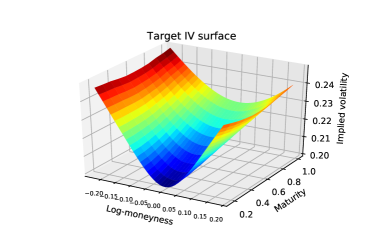
Figure B.1. The “market” data used in calibration of the Neural SDE models. In fact the implied volatility surface comes from (B.1) and (B.4).

Options with bi-monthly maturities up to one year with varying range of strikes were used as market data for Neural SDE calibration. The call / put option prices were obtained from the Heston model using Monte Carlo simulation with $10^{7}$ Brownian trajectories. We use bimonthly maturities up to one year for considered calibrations. Varying range of strikes is used among different calibrations. See Figure B.1 for the resulting “market” data.

Appendix C Feed-forward neural networks

Feed-forward neural networks are functions constructed by composition of affine map and non-linear activation function. We fix a locally Lipschitz activation function $\mathbf{a}:\mathbb{R}\to\mathbb{R}$ as ReLU function $a(z)=(0,z)_{+}$ and for $d\in\mathbb{N}$ define $\mathbf{A}_{d}:\mathbb{R}^{d}\to\mathbb{R}^{d}$ as the function given, for $x=(x_{1},\ldots,x_{d})$ by $\mathbf{A}_{d}(x)=(\mathbf{a}(x_{1}),\ldots,\mathbf{a}(x_{d}))$. We fix $L\in\mathbb{N}$ (the number of layers), $l_{k}\in\mathbb{N}$, $k=0,1,\ldots L-1$ (the size of input to layer $k$) and $l_{L}\in\mathbb{N}$ (the size of the network output). A fully connected artificial neural network is then given by $\theta=((W_{1},B_{1}),\ldots,(W_{L},B_{L}))$, where, for $k=1,\ldots,L$, we have real $l_{k-1}\times l_{k}$ matrices $W_{k}$ and real $l_{k}$ dimensional vectors $B_{k}$.

The artificial neural network defines a function $\mathcal{R}(\cdot,\theta):\mathbb{R}^{l_{0}}\to\mathbb{R}^{l_{L}}$ given recursively, for $x_{0}\in\mathbb{R}^{l_{0}}$, by

$$\mathcal{R}(x_{0},\theta)=W_{L}x_{L-1}+B_{L}\,,\,\,\,\,x_{k}=\mathbf{A}_{l_{k}}(W_{k}x_{k-1}+B_{k})\,,k=1,\ldots,L-1\,.$$

We will call such class of fully connected artificial neural networks $\mathcal{DN}$. Note that since the activation functions and architecture are fixed the learning task entails finding the optimal $\theta\in\mathbb{R}^{\mathcal{P}}$ where $p$ is the number of parameters in $\theta$ given by

$$\mathcal{P}(\theta)=\sum_{i=1}^{L}(l_{k-1}l_{k}+l_{k})\,.$$

Appendix D LV neural SDEs calibration accuracy

Figures 5.2, D.2, D.4 present implied volatility fit of local volatility neural SDE model (5.2) calibrated to: market vanilla data only; market vanilla data with lower bound constraint on lookback option payoff; market vanilla data with upper bound constraint on lookback option payoff respectively. Figures D.1, D.3, D.5 present target option price fit of local volatility neural SDE model (5.2) calibrated to: market vanilla data only; market vanilla data with lower bound constraint on lookback option payoff; market vanilla data with upper bound constraint on lookback option payoff respectively. High level of accuracy in all calibrations is achieved due to the hedging neural network incorporated into model training.

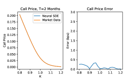
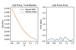
Figure D.1. Calibrated neural SDE LV model and market target prices comparison.

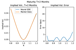
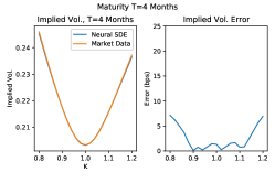
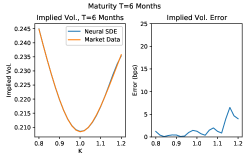
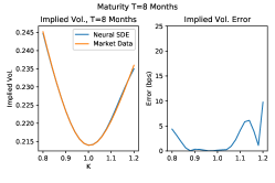
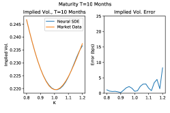
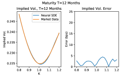
Figure D.2. Calibrated neural SDE LV model (with lower bound minimization on exotic payoff) and target market data implied volatility comparison.

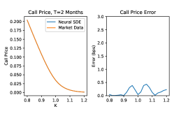
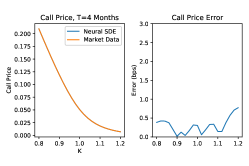
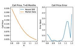
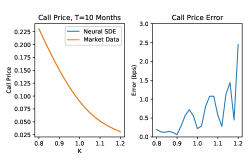
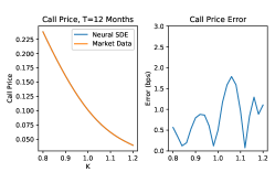
Figure D.3. Calibrated neural SDE LV model (with lower bound minimization on exotic payoff) and target market prices comparison.

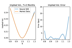
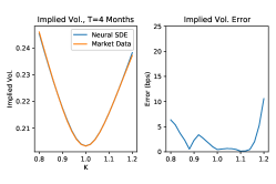
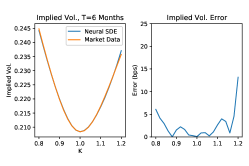
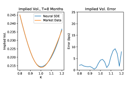
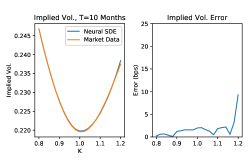
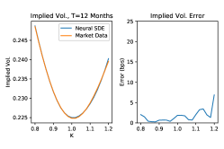
Figure D.4. Calibrated neural LV model (with upper bound maximization on exotic payoff) and target market data implied volatility comparison.

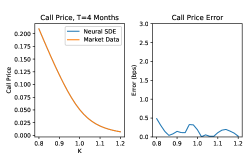
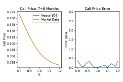
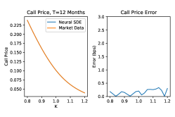
Figure D.5. Calibrated LV neural model (with upper bound maximization on exotic payoff) and target market prices comparison.

Appendix E LSV neural SDEs calibration accuracy

Figures E.1, 5.4 and E.2 provide the Vanilla call option price and the implied volatility curve for the calibrated models. In each plot, the blue line corresponds to the target data (generated using Heston model), and each orange line corresponds to one run of the Neural SDE calibration. We note again in this plots how the absolute error of the calibration to the vanilla prices is consistently of $\mathcal{O}(10^{-4})$.

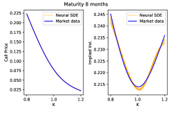
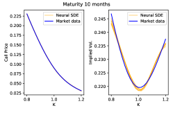
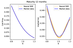
Figure E.1. Comparing market and model data fit for the Neural SDE LSV model (5.3) when targeting the lower bound on the illiquid derivative. We see vanilla option prices and implied volatility curves of the 10 calibrated Neural SDEs vs. the market data for different maturities.

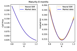
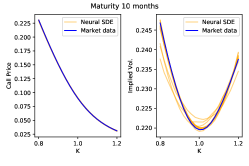
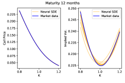
Figure E.2. Comparing market and model data fit for the Neural SDE LSV model (5.3) when targeting the upper bound on the illiquid derivative. We see vanilla option prices and implied volatility curves of the 10 calibrated Neural SDEs vs. the market data for different maturities.

Appendix F Exotic price in LV neural SDEs

Below we see how different random seeds, constrained optimization algorithms and number of strikes used in the market data input affect the illiquid derivative price in the Local Volatility Neural SDE model.

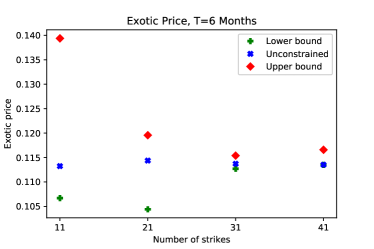
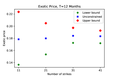
Figure F.1. Lookback exotic option price in lower, upper and unconstrained implied by perfectly calibrated LV neural SDE calibrated to varying number of market option quotes.

Initialisation	Calibration type	t=2/12	t=4/12	t=6/12	t=8/12	t=10/12	t=1
1	Unconstrained	.055	.088	.113	.134	.159	.178
2	Unconstrained	.056	.086	.113	.132	.158	.175
1	LB Lag. mult.	.055	.086	.107	.127	.143	.154
2	LB Lag. mult.	.055	.084	.098	.113	.125	.139
1	UB Lag. mult.	.056	.099	.119	.142	.163	.214
2	UB Lag. mult.	.059	.101	.131	.156	.208	.220
1	LB Augmented	.055	.077	.107	.113	.127	.136
2	LB Augmented	.056	.085	.109	.123	.139	.158
1	UB Augmented	.058	.102	.139	.156	.188	.224
2	UB Augmented	.057	.088	.128	.151	.167	.184
-	Heston 400k paths	.058	.087	.111	.133	.154	.174

Table 1. Impact of initialisation and constrained optimization algorithms on prices of an illiquid derivative (lookback call) implied by LV neural SDE calibrated to vanilla prices with $K=11$ strikes: $k_{1}=0.9,k_{2}=0.92,...,k_{11}=1.1$ for each maturity.

Initialisation	Calibration type	t=2/12	t=4/12	t=6/12	t=8/12	t=10/12	t=1
1	Unconstrained	.056	.087	.114	.140	.161	.182
2	Unconstrained	.056	.087	.114	.136	.161	.180
1	LB Lag. mult.	.056	.086	.110	.123	.141	.153
2	LB Lag. mult.	.056	.087	.108	.125	.150	.155
1	UB Lag. mult.	.056	.088	.120	.156	.179	.205
2	UB Lag. mult.	.056	.088	.118	.153	.187	.208
1	LB Augmented	.056	.087	.108	.128	.143	.164
2	LB Augmented	.056	.087	.108	.125	.150	.155
1	UB Augmented	.056	.091	.124	.155	.173	.194
2	UB Augmented	.056	.088	.125	.146	.167	.189
-	Heston 400k paths	.058	.087	.111	.133	.154	.174
-	Heston 10mil paths	.058	.087	.111	.133	.154	.174

Table 2. Impact of initialisation Prices of ATM lookback call implied by LV neural SDE calibrated to vanilla prices with $K=21$ strikes: $k_{1}=0.8,k_{2}=0.82,...,k_{21}=1.2$ for each maturity.

Initialisation	Calibration type	t=2/12	t=4/12	t=6/12	t=8/12	t=10/12	t=1
1	Unconstrained	.056	.087	.114	.138	.162	.184
2	Unconstrained	.056	.087	.114	.138	.160	.183
1	LB Lag. mult.	.056	.087	.113	.137	.149	.172
2	LB Lag. mult.	.056	.087	.113	.136	.155	.165
1	UB Lag. mult.	.056	.088	.115	.148	.170	.197
2	UB Lag. mult.	.056	.087	.114	.144	.170	.198
1	LB Augmented	.056	.087	.114	.138	.161	.183
2	LB Augmented	.056	.087	.112	.130	.154	.166
1	UB Augmented	.056	.087	.114	.138	.162	.183
2	UB Augmented	.056	.087	.114	.141	.164	.190
-	Heston 400k paths	.058	.087	.111	.133	.154	.174
-	Heston 10mil paths	.058	.087	.111	.133	.154	.174

Table 3. Impact of initialisation Prices of ATM lookback call implied by LV neural SDE calibrated to vanilla prices with $K=31$ strikes: $k_{1}=0.7,k_{2}=0.72,...,k_{31}=1.3$ for each maturity.

Initialisation	Calibration type	t=2/12	t=4/12	t=6/12	t=8/12	t=10/12	t=1
1	Unconstrained	.056	.087	.114	.138	.160	.183
2	Unconstrained	.056	.087	.113	.138	.162	.184
1	LB Lag. mult.	.056	.087	.113	.137	.158	.172
2	LB Lag. mult.	.056	.087	.113	.137	.153	.171
1	UB Lag. mult.	.056	.088	.117	.141	.166	.193
2	UB Lag. mult.	.056	.087	.116	.140	.166	.192
1	LB Augmented	.056	.087	.113	.136	.153	.172
2	LB Augmented	.056	.087	.113	.136	.152	.169
1	UB Augmented	.056	.087	.114	.138	.160	.182
2	UB Augmented	.056	.087	.116	.140	.164	.191
-	Heston 400k paths	.058	.087	.111	.133	.154	.174
-	Heston 10mil paths	.058	.087	.111	.133	.154	.174

Table 4. Impact of initialisation Prices of ATM lookback call implied by LV neural SDE calibrated to vanilla prices with $K=41$ strikes: $k_{1}=0.6,k_{2}=0.62,...,k_{41}=1.4$ for each maturity.

References

• [Acciaio et al., 2019] Acciaio, B., Backhoff-Veraguas, J., and Zalashko, A. (2019). Causal optimal transport and its links to enlargement of filtrations and continuous-time stochastic optimization. Stochastic Processes and their Applications.
• [Aksamit et al., 2020] Aksamit, A., Hou, Z., and Obloj, J. (2020). Robust framework for quantifying the value of information in pricing and hedging. SIAM Journal on Financial Mathematics, 11(1):27–59.
• [Albrecher et al., 2007] Albrecher, H., Mayer, P., Schoutens, W., and Tistaert, J. (2007). The little heston trap. Wilmott, pages 83–92.
• [Bayer et al., 2019] Bayer, C., Horvath, B., Muguruza, A., Stemper, B., and Tomas, M. (2019). On deep calibration of (rough) stochastic volatility models.
• [Bayer and Stemper, 2018] Bayer, C. and Stemper, B. (2018). Deep calibration of rough stochastic volatility models.
• [Beiglböck et al., 2013] Beiglböck, M., Henry-Labordère, P., and Penkner, F. (2013). Model-independent bounds for option prices—a mass transport approach. Finance and Stochastics, 17(3):477–501.
• [Benth et al., 2020] Benth, F. E., Detering, N., and Lavagnini, S. (2020). Accuracy of deep learning in calibrating HJM forward curves. arXiv preprint arXiv:2006.01911.
• [Benveniste et al., 2012] Benveniste, A., Métivier, M., and Priouret, P. (2012). Adaptive algorithms and stochastic approximations, volume 22. Springer Science & Business Media.
• [Broadie et al., 2011] Broadie, M., Du, Y., and Moallemi, C. C. (2011). Efficient risk estimation via nested sequential simulation. Management Science, 57(6):1172–1194.
• [Buehler et al., 2019] Buehler, H., Gonon, L., Teichmann, J., and Wood, B. (2019). Deep hedging. Quantitative Finance, pages 1–21.
• [Chassagneux et al., 2019] Chassagneux, J.-F., Szpruch, L., and Tse, A. (2019). Weak quantitative propagation of chaos via differential calculus on the space of measures. arXiv:1901.02556.
• [Cohen and Elliott, 2015] Cohen, S. N. and Elliott, R. J. (2015). Stochastic calculus and applications, volume 2. Springer.
• [Cohen et al., 2018] Cohen, S. N. et al. (2018). Data and uncertainty in extreme risks-a nonlinear expectations approach. World Scientific Book Chapters, pages 135–162.
• [Cox and Obloj, 2011] Cox, A. M. and Obloj, J. (2011). Robust hedging of double touch barrier options. SIAM Journal on Financial Mathematics, 2(1):141–182.
• [Cuchiero et al., 2020] Cuchiero, C., Khosrawi, W., and Teichmann, J. (2020). A generative adversarial network approach to calibration of local stochastic volatility models. arXiv preprint arXiv:2005.02505.
• [Cuchiero et al., 2019] Cuchiero, C., Larsson, M., and Teichmann, J. (2019). Deep neural networks, generic universal interpolation, and controlled odes. arXiv preprint arXiv:1908.07838.
• [Dupire et al., 1994] Dupire, B. et al. (1994). Pricing with a smile. Risk, 7(1):18–20.
• [Eckstein et al., 2019] Eckstein, S., Guo, G., Lim, T., and Obloj, J. (2019). Robust pricing and hedging of options on multiple assets and its numerics. arXiv preprint arXiv:1909.03870.
• [Eckstein and Kupper, 2019] Eckstein, S. and Kupper, M. (2019). Computation of optimal transport and related hedging problems via penalization and neural networks. Applied Mathematics & Optimization, pages 1–29.
• [Fournié et al., 1999] Fournié, E., Lasry, J.-M., Lebuchoux, J., Lions, P.-L., and Touzi, N. (1999). Applications of malliavin calculus to monte carlo methods in finance. Finance and Stochastics, 3(4):391–412.
• [Gambara and Teichmann, 2020] Gambara, M. and Teichmann, J. (2020). Consistent recalibration models and deep calibration. arXiv preprint arXiv:2006.09455.
• [Glasserman, 2013] Glasserman, P. (2013). Monte Carlo methods in financial engineering, volume 53. Springer Science & Business Media.
• [Goodfellow et al., 2014] Goodfellow, I., Pouget-Abadie, J., Mirza, M., Xu, B., Warde-Farley, D., Ozair, S., Courville, A., and Bengio, Y. (2014). Generative adversarial nets. In Advances in neural information processing systems, pages 2672–2680.
• [Gyöngy, 1986] Gyöngy, I. (1986). Mimicking the one-dimensional marginal distributions of processes having an itô differential. Probability theory and related fields, 71(4):501–516.
• [Hammersley et al., 2019] Hammersley, W. R., Šiška, D., and Szpruch, Ł. (2019). Weak existence and uniqueness for mckean-vlasov sdes with common noise. arXiv preprint arXiv:1908.00955.
• [Hernandez, 2016] Hernandez, A. (2016). Model calibration with neural networks. Risk.
• [Hestenes, 1969] Hestenes, M. R. (1969). Multiplier and gradient methods. Journal of optimization theory and applications, 4(5):303–320.
• [Heston, 1997] Heston, S. L. (1997). A closed-form solution for options with stochastic volatility and applications to bond and currency options. The Review of Financial Studies, 6:327–343.
• [Hobson, 1998] Hobson, D. G. (1998). Robust hedging of the lookback option. Finance and Stochastics, 2(4):329–347.
• [Hornik, 1991] Hornik, K. (1991). Approximation capabilities of multilayer feedforward networks. Neural Networks, 4(2):251–257.
• [Horvath et al., 2019] Horvath, B., Muguruza, A., and Tomas, M. (2019). Deep learning volatility.
• [Hutzenthaler et al., 2011] Hutzenthaler, M., Jentzen, A., and Kloeden, P. E. (2011). Strong and weak divergence in finite time of euler’s method for stochastic differential equations with non-globally lipschitz continuous coefficients. Proceedings of the Royal Society A: Mathematical, Physical and Engineering Sciences, 467(2130):1563–1576.
• [Hutzenthaler et al., 2012] Hutzenthaler, M., Jentzen, A., Kloeden, P. E., et al. (2012). Strong convergence of an explicit numerical method for sdes with nonglobally lipschitz continuous coefficients. The Annals of Applied Probability, 22(4):1611–1641.
• [Jabir et al., 2019] Jabir, J.-F., Šiška, D., and Szpruch, Ł. (2019). Mean-field neural odes via relaxed optimal control. arxiv preprint arXiv:1912.05475.
• [Karatzas and Shreve, 2012] Karatzas, I. and Shreve, S. (2012). Brownian motion and stochastic calculus. Springer.
• [Kingma and Ba, 2014] Kingma, D. P. and Ba, J. (2014). Adam: A method for stochastic optimization. arXiv preprint arXiv:1412.6980.
• [Kingma and Welling, 2013] Kingma, D. P. and Welling, M. (2013). Auto-encoding variational bayes. arXiv preprint arXiv:1312.6114.
• [Knight, 1971] Knight, F. H. (1971). Risk, uncertainty and profit, 1921. Library of Economics and Liberty.
• [Krylov, 1999] Krylov, N. (1999). On kolmogorov’s equations for finite dimensional diffusions. In Stochastic PDE’s and Kolmogorov Equations in Infinite Dimensions, pages 1–63. Springer.
• [Krylov, 1980] Krylov, N. V. (1980). Controlled diffusion processes, volume 14 of Applications of Mathematics. Springer-Verlag, New York-Berlin. Translated from the Russian by A. B. Aries.
• [Kunita, 1997] Kunita, H. (1997). Stochastic flows and stochastic differential equations, volume 24. Cambridge university press.
• [Lassalle, 2013] Lassalle, R. (2013). Causal transference plans and their monge-kantorovich problems. arXiv preprint arXiv:1303.6925.
• [Liu et al., 2019] Liu, S., Borovykh, A., Grzelak, L. A., and Oosterlee, C. W. (2019). A neural network-based framework for financial model calibration. Journal of Mathematics in Industry, 9(1):9.
• [Majka et al., 2020] Majka, M. B., Sabate-Vidales, M., and Szpruch, Ł. (2020). Multi-index antithetic stochastic gradient algorithm. arXiv preprint arXiv:2006.06102.
• [Nadtochiy and Obloj, 2017] Nadtochiy, S. and Obloj, J. (2017). Robust trading of implied skew. International Journal of Theoretical and Applied Finance, 20(02):1750008.
• [Paszke et al., 2017] Paszke, A., Gross, S., Chintala, S., Chanan, G., Yang, E., DeVito, Z., Lin, Z., Desmaison, A., Antiga, L., and Lerer, A. (2017). Automatic differentiation in pytorch.
• [Paszke et al., 2019] Paszke, A., Gross, S., Massa, F., Lerer, A., Bradbury, J., Chanan, G., Killeen, T., Lin, Z., Gimelshein, N., Antiga, L., et al. (2019). Pytorch: An imperative style, high-performance deep learning library. In Advances in Neural Information Processing Systems, pages 8024–8035.
• [Pelsser and Schweizer, 2016] Pelsser, A. and Schweizer, J. (2016). The difference between lsmc and replicating portfolio in insurance liability modeling. European actuarial journal, 6(2):441–494.
• [Ruf and Wang, 2019] Ruf, J. and Wang, W. (2019). Neural networks for option pricing and hedging: a literature review. Available at SSRN 3486363.
• [Sardroudi, 2019] Sardroudi, W. K. (2019). Polynomial semimartingales and a deep learning approach to local stochastic volatility calibration.
• [Šiška and Szpruch, 2020] Šiška, D. and Szpruch, Ł. (2020). Gradient flows for regularized stochastic control problems. arxiv preprint arXiv:2006.05956.
• [Sontag and Sussmann, 1997] Sontag, E. and Sussmann, H. (1997). Complete controllability of continuous-time recurrent neural networks. Systems Control Lett., 30(4):177–183.
• [Srivastava et al., 2014] Srivastava, N., Hinton, G., Krizhevsky, A., Sutskever, I., and Salakhutdinov, R. (2014). Dropout: a simple way to prevent neural networks from overfitting. The journal of machine learning research, 15(1):1929–1958.
• [Szpruch and Zhāng, 2018] Szpruch, Ł. and Zhāng, X. (2018). $V$-integrability, asymptotic stability and comparison property of explicit numerical schemes for non-linear SDEs. Math. Comp., 87(310):755–783.
• [Tian et al., 2015] Tian, Y., Zhu, Z., Lee, G., Klebaner, F., and Hamza, K. (2015). Calibrating and pricing with a stochastic-local volatility model. The Journal of Derivatives, 22(3):21–39.
• [Vidales et al., 2018] Vidales, M. S., Šiška, D., and Szpruch, L. (2018). Unbiased deep solvers for parametric PDEs. arXiv:1810.05094.
• [Vidales et al., 2020] Vidales, M. S., Šiška, D., and Szpruch, L. (2020). Learning solutions to path dependent PDEs with signatures and LSTM networks. In preparation.