Local distributions of the 1D dilute Ising model

Abstract

The local distributions of the one-dimensional dilute annealed Ising model with charged impurities are studied. Explicit expressions are obtained for the pair distribution functions and correlation lengths, and their low-temperature asymptotic behavior is explored depending on the concentration of impurities. For a more detailed consideration of the ordering processes, we study local distributions. Based on the Markov property of the dilute Ising chain, we obtain an explicit expression for the probability of any finite sequence and find a geometric probability distribution for the lengths of sequences consisting of repeating blocks. An analysis of distributions shows that the critical behavior of the spin correlation length is defined by ferromagnetic or antiferromagnetic sequences, while the critical behavior of the impurity correlation length is defined by the sequences of impurities or by the charge-ordered sequences. For the dilute Ising chain, there are no other repeating sequences whose mean length diverges at zero temperature. While both the spin correlation and the impurity correlation lengths can diverge only at zero temperature, the ordering processes result in a maximum of the specific heat at finite temperature defined by the maximum rate of change of the impurity-spin pairs concentration. A simple approximate equation is found for this temperature. We show that the non-ordered dilute Ising chains correspond to the regular Markov chains, while various orderings generate the irregular Markov chains of different types.

I Introduction

One-dimensional (1D) spin models, including Ising type ones, are convenient objects for testing both the basic concepts of statistical physics and the applicability of new methods. To date, exact solutions have been found for various complex models based on the 1D Ising model. They includes Blume-Emery-Griffiths model Wu1978 ; Thomaz2016 ; CorreaSilva2016 , the model with localized Ising-like spins and exchanging electrons Pereira2008 , the models with single-ion anisotropy for the spin-1 chain Yang2008 ; Yang2009 ; DeSouza2014 or the mixed spin-1/2 and spin-1 Ising chain Wu2010 ; Wu2011 ; Strecka2011 , the Ising-Heisenberg “decorated” chains, ladders, and tubes Canova2006 ; Antonosyan2009 ; Rojas2011 ; Galisova2013 ; Torrico2014 ; Lisnyi2015 ; Galisova2015 ; Rojas2016 ; Strecka2016 ; Torrico2018 and the Ising-Hubbard diamond chain and ladder Lisnii2011 ; Sousa2018 . These systems show many subtle and important phenomena, including quantized plateaux in the magnetization curves, quantum entanglement, quasi-phases and pseudo-transitions DeSouza2018 , and describe the properties of real materials, such as the polymeric coordination compounds (see Refs. in Antonosyan2009 ; Strecka2011 ; Rojas2016 ; Strecka2016 ; Torrico2018 ; Sousa2018 ). At the same time, the analysis of the conventional 1D Ising model also continues taking into account higher spin $S$ values Suzuki1967 , two kinds of spins Muto1976 , the random short- and long-range interactions Haley1978 ; Goncalves1998 , the next-nearest-neighbour coupling Fakhri2019 and the magnetic field Kassan-ogly2001 ; Proshkin2017 ; Zarubin2019 .

The dilute Ising model is one of the basic ones in the theory of magnetic systems disordered by non-magnetic impurities. Undoubtedly, the 1D version of this model has a long history. The energy and susceptibility for non-interacting impurities was obtained by Katsura and Tsujiyama Katsura1965 and the expressions of thermodynamic functions on the impurities density was given by Kawatra and Kijewski Kawatra1969 . The exact solution and various thermodynamic properties of the dilute Ising chain with interacting impurities was found in Rys1969 ; Matsubara1973 ; Termonia1974 and in the most general form by Balagurov, Vaks and Zaitsev in Balagurov1974 . However, despite a long history, the local distributions of spins and non-magnetic interacting impurities in the 1D dilute Ising model have not been described systematically as yet. The size distribution of clusters is of fundamental interest and has been studied intensively in the Ising or similar models Wortis1974 ; Vaks1975 ; Harris1975 ; Binder1976 ; Marro1983 ; Thomsen1983 ; Toral1987 ; Hu1986 ; Khn1987 ; Vavro2001 ; Campi2003 ; Yilmaz2005 ; Simonin2013 .

In the present paper, we consider the distributions properties of charged non-magnetic impurities and spins for the 1D dilute Ising model. From a general point of view, the distributions considered here reveal the reason for the lack of ordering in the 1D dilute Ising model at finite temperature.

The paper is organized as follows. In section 2, we obtain the pair distribution functions, the correlation lengths, and the probabilities of local distributions in the dilute Ising chain. Often local distributions are considered as a way to calculate the thermodynamics of the entire system, so initially, one uses their combinatorial probabilities Wortis1974 ; Binder1976 ; Thomsen1983 . Based on the Markov property of the dilute Ising chain, we calculate the thermodynamic probabilities, obtaining them from the pair distribution functions. Especially, we find the type of the probability distribution for the lengths of sequences of repeated blocks. Section 3 describes the features of the ordering processes at low temperatures for various model parameters. Given the properties of correlation lengths, we examine the distributions for several specific types of local sequences and prove the absence of other sequences with diverging mean length. In the end, we discuss the properties of the Markov chains, which are generated by the ordered and non-ordered dilute Ising chains. Conclusions are presented in section 4.

II Theory

II.1 Pair distribution functions and correlation lengths

In this work, we consider the dilute Ising chain, which has the Hamiltonian

$$\mathcal{H}=-J\sum_{j=1}^{N}\sigma_{j}\sigma_{j+1}+V\sum_{j=1}^{N}P_{0,j}P_{0,j+1}-\mu\sum_{j=1}^{N}P_{0,j}.$$ (1)

Here the pseudospin $\sigma=1$ operator is used, where the states of conventional spin doublet and non-magnetic impurity correspond to the pseudospin $z$-projections $\sigma=\pm 1$ and $\sigma=0$, respectively, $J$ is the exchange constant, $V$ is the inter-site interaction for impurities, $P_{0}=1-\sigma^{2}$ is the projection operator onto the $\sigma=0$ state, and $\mu$ is the chemical potential. Further we will assume that nonmagnetic impurities are mobile, which corresponds to the annealed system.

Detailed information on the state of the thermodynamic system is provided by the pair distribution functions (PDF) $\left\langle P_{a,k}\,P_{b,k+l}\right\rangle$, where $P_{a,k}$ is the projection operator on one of the basis state, $a=\pm,0$ for $\sigma=\pm 1,0$. PDF of the 1D dilute Ising model can be calculated by

$$\left\langle P_{a,k}\,P_{b,k+l}\right\rangle=\lim_{N\to\infty}\frac{\mathop{\mathrm{Tr}}\left(P_{a}\mathcal{T}^{l}P_{b}\mathcal{T}^{N-l}\right)}{\mathop{\mathrm{Tr}}\left(\mathcal{T}^{N}\right)}.$$ (2)

Here $\mathcal{T}$ is the transfer matrix for Hamiltonian (1) at $h=0$

$$\mathcal{T}=\left(\begin{array}[]{ccc}e^{K}&e^{\xi/2}&e^{-K}\\ e^{\xi/2}&e^{-W+\xi}&e^{\xi/2}\\ e^{-K}&e^{\xi/2}&e^{K}\end{array}\right),$$ (3)

where $K=\beta J$, $W=\beta V$, $\xi=\beta\mu$, $\beta=1/\theta$ and $\theta=k_{B}T$. The activity can be expressed at given concentration of impurities $n$ as

$$e^{\xi}=2\,\frac{g+m}{g-m}\,e^{W}\cosh K,$$ (4)

where $m=n-1/2$ is the deviation of the concentration of impurities from half-filling and

$$g=\left[m^{2}+\left(\frac{1}{4}-m^{2}\right)e^{-W}\cosh K\right]^{1/2}.$$ (5)

From (2) we obtain

$$\langle P_{0,k}P_{0,k+l}\rangle = \left(\frac{1}{2}+m\right)^{2}+\left(\frac{1}{4}-m^{2}\right)\Lambda_{0}^{l},$$ (6)

$$\langle P_{0,k}P_{\pm,k+l}\rangle = \frac{1}{2}\left(\frac{1}{4}-m^{2}\right)\left(1-\Lambda_{0}^{l}\right),$$ (7)

$$\langle P_{\pm,k}P_{\pm,k+l}\rangle = \frac{1}{4}\bigg{[}\left(\frac{1}{2}-m\right)^{2}+\left(\frac{1}{4}-m^{2}\right)\Lambda_{0}^{l}+{}$$ (8)

$${}+\left(\frac{1}{2}-m\right)\Lambda_{\sigma}^{l}\bigg{]},$$

$$\langle P_{\pm,k}P_{\mp,k+l}\rangle = \frac{1}{4}\bigg{[}\left(\frac{1}{2}-m\right)^{2}+\left(\frac{1}{4}-m^{2}\right)\Lambda_{0}^{l}-{}$$ (9)

$${}-\left(\frac{1}{2}-m\right)\Lambda_{\sigma}^{l}\bigg{]},$$

where

$$\Lambda_{0}=\frac{2g-1}{2g+1},\qquad\Lambda_{\sigma}=\frac{g-m}{g+\frac{1}{2}}\,\tanh K.$$ (10)

In all cases, we have

$$\left\langle P_{a,k}\,P_{b,k+l}\right\rangle=\left\langle P_{a}\right\rangle\left\langle P_{b}\right\rangle+K_{ab}(l),$$ (11)

where $\left\langle P_{0}\right\rangle=\frac{1}{2}+m$, $\left\langle P_{\pm}\right\rangle=\frac{1}{2}\left(\frac{1}{2}-m\right)$, and $K_{ab}(l)$ is the correlation function for the states $a$ and $b$.

Using the projection operator on the states of the spin doublet, $P_{1}=P_{+}+P_{-}$, we obtain additional PDF:

$$\langle P_{0,k}P_{1,k+l}\rangle = \left(\frac{1}{4}-m^{2}\right)\left(1-\Lambda_{0}^{l}\right),$$ (12)

$$\langle P_{1,k}P_{1,k+l}\rangle = \left(\frac{1}{2}-m\right)^{2}+\left(\frac{1}{4}-m^{2}\right)\Lambda_{0}^{l}.$$ (13)

From the identity $\sigma=P_{+}-P_{-}$ we find the spin-spin correlation function:

$$\langle\sigma_{k}\sigma_{k+l}\rangle=\left(\frac{1}{2}-m\right)\Lambda_{\sigma}^{l}.$$ (14)

Assuming that $\langle\sigma_{k}\sigma_{k+l}\rangle\propto e^{-l/\ell}$, we find the expression for the spin correlation length $\ell$:

$$\ell^{-1}=\ln\left|\Lambda_{\sigma}^{-1}\right|=\ell_{Is}^{-1}+\tilde{\ell}^{-1},\qquad\tilde{\ell}^{-1}=\ln\frac{g+\frac{1}{2}}{g-m}.$$ (15)

Here $\ell_{Is}$ is the spin correlation length of the pure Ising chain, and $\tilde{\ell}$ is the additive due to impurities. The emergence of $\tilde{\ell}$ decreases the spin correlation length $\ell$.

Writing the impurity correlation function in the form $K_{00}(l)\propto e^{-l/\ell_{0}}$, we find the impurity correlation length $\ell_{0}$:

$$\ell_{0}^{-1}=\ln\left|\Lambda_{0}^{-1}\right|.$$ (16)

If $V<|J|$, the function $\Lambda_{0}$ changes the sign from negative at high temperatures to positive at low temperatures. This means that the tendency to the charge ordering of impurities at high temperatures is replaced by a tendency to a homogeneous distribution at low temperatures. The temperature, when $\Lambda_{0}=0$, is obtained from the equation $e^{|K|}=e^{W}+\left(e^{2W}-1\right)^{1/2}$. When $V\geq|J|$, the function $\Lambda_{0}$ is always negative.

II.2 Probability distributions for the finite sequences

PDF $\left\langle P_{a,k}P_{b,k+1}\right\rangle$ equals to the probability for the nearest neighbors to be in the states $a$ and $b$ simultaneously, $P(ab)$. Using Bayes’s formula, it can be represented as

$$\left\langle P_{a,k}P_{b,k+1}\right\rangle\equiv P(ab)=P(a)P(b|a)=P(a|b)P(b),$$ (17)

where $P(\sigma)$ is the probability for $k$th site to be in the state $\sigma$, $P(\sigma^{\prime}|\sigma)$ is the conditional probability of the state $\sigma^{\prime}$ on $(k{+}1)$st site, given that $k$th site is in the state $\sigma$. The conditional probabilities for the states with $\sigma={+}1,0,{-}1$ can be written as a non-symmetric matrix with the elements $\mathcal{P}_{ab}=P(a|b)$:

$$\mathcal{P}=\frac{1}{2g{+}1}\begin{pmatrix}\displaystyle\frac{(g{-}m)e^{K}}{\cosh K}&\displaystyle\frac{1}{2}-m&\displaystyle\frac{(g{-}m)e^{-K}}{\cosh K}\\[10.00002pt] \displaystyle 1+2m&\displaystyle 2(g{+}m)&\displaystyle 1+2m\\[5.0pt] \displaystyle\frac{(g{-}m)e^{-K}}{\cosh K}&\displaystyle\frac{1}{2}-m&\displaystyle\frac{(g{-}m)e^{K}}{\cosh K}\end{pmatrix}.$$ (18)

$\mathcal{P}$ is a left stochastic matrix and it has eigenvalues 1, $\Lambda_{0}$ and $\Lambda_{\sigma}$. The eigenvector for the eigenvalue 1 is proportional to the equilibrium distribution for the states of the dilute Ising chain $\left(\frac{1}{2}\left(\frac{1}{2}{-}m\right),\,\frac{1}{2}{+}m,\,\frac{1}{2}\left(\frac{1}{2}{-}m\right)\right)$. This means that the dilute Ising chain corresponds to the Markov chain with the transition matrix $\mathcal{P}^{T}$. To verify this, one can check that PDF (6-9) are expressed in terms of the $l$th power of the matrix $\mathcal{P}$:

$$\left\langle P_{a,k}P_{b,k+l}\right\rangle=$$

$$\quad=\sum_{\sigma_{1},\ldots,\sigma_{l-1}}P(a|\sigma_{1})P(\sigma_{1}|\sigma_{2})\ldots P(\sigma_{l-1}|b)P(b)$$

$$\quad=\mathcal{P}^{l}_{ab}P(b)\;=\;\mathcal{P}^{l}_{ba}P(a).$$ (19)

This is a consequence of the Chapman-Kolmogorov equations. The Markov property for the pure Ising system is well-known Malyshev1991 . Similarly, PDF (6,12,13) can be calculated using the $l$th power of the conditional probability matrix for the states 0 (impurity) and 1 (magnetic):

$$\mathcal{P}^{\prime}=\frac{2}{2g+1}\left(\begin{array}[]{cc}\displaystyle g+m&\displaystyle\frac{1}{2}+m\\ \displaystyle\frac{1}{2}-m&\displaystyle g-m\end{array}\right).$$ (20)

The Markov property allows us to calculate the probability of any given sequence of states $(ab\ldots cd)$ for the sites following each other in a dilute Ising chain using the matrix elements of $\mathcal{P}$ or $\mathcal{P}^{\prime}$:

$$P(ab\ldots cd) = P(a|b)\ldots P(c|d)P(d)$$ (21)

$$= P(d|c)\ldots P(b|a)P(a).$$

Now consider an isolated sequence consisting of $l$ repeating blocks $\boldsymbol{\sigma}$, where $\boldsymbol{\sigma}=(\sigma_{1}\ldots\sigma_{n})$. The probability that this sequence exists is

$$P_{l}(\boldsymbol{\sigma})=\sum_{\boldsymbol{\sigma}^{\prime}\neq\boldsymbol{\sigma},\boldsymbol{\sigma}^{\prime\prime}\neq\boldsymbol{\sigma}}P(\boldsymbol{\sigma}^{\prime}\boldsymbol{\sigma}^{l}\boldsymbol{\sigma}^{\prime\prime})=P_{1}(\boldsymbol{\sigma})\,q_{\boldsymbol{\sigma}}^{l-1},$$ (22)

where

$$q_{\boldsymbol{\sigma}}=P(\sigma_{1}|\sigma_{2})\ldots P(\sigma_{n}|\sigma_{1}),$$ (23)

$$P_{1}(\boldsymbol{\sigma})=\sum_{\boldsymbol{\sigma}^{\prime}\neq\boldsymbol{\sigma},\boldsymbol{\sigma}^{\prime\prime}\neq\boldsymbol{\sigma}}P(\boldsymbol{\sigma}^{\prime}\boldsymbol{\sigma}\boldsymbol{\sigma}^{\prime\prime}).$$ (24)

Here $q_{\boldsymbol{\sigma}}$ can be treated as the probability of a cyclic sequence consisting of sites $\sigma_{1}\ldots\sigma_{n}$ and the accounting of equation (21) gives inequality $q_{\boldsymbol{\sigma}}<P(\boldsymbol{\sigma})$. $P_{1}(\boldsymbol{\sigma})$ is the probability of an isolated block $\boldsymbol{\sigma}$, and calculating the sum in (24) we get

$$P_{1}(\boldsymbol{\sigma})=\left(1-q_{\boldsymbol{\sigma}}\right)^{2}P(\boldsymbol{\sigma}).$$ (25)

Equation (25) generalizes the result of Yilmaz and Zimmermann Yilmaz2005 for a pure Ising chain. The sum of $P_{l}(\boldsymbol{\sigma})$ over $l$ is the total probability of the boundary configurations $(\boldsymbol{\sigma}^{\prime}\boldsymbol{\sigma})$:

$$\sum_{l=1}^{\infty}P_{l}(\boldsymbol{\sigma})=\sum_{\boldsymbol{\sigma}^{\prime}\neq\boldsymbol{\sigma}}P(\boldsymbol{\sigma}^{\prime}\boldsymbol{\sigma})=\left(1-q_{\boldsymbol{\sigma}}\right)P(\boldsymbol{\sigma}).$$ (26)

Using the quantity (26) as a normalization factor, we obtain the probability distribution for the lengths $l$ of sequences of repeating blocks $\boldsymbol{\sigma}$:

$$p_{l}(\boldsymbol{\sigma})=\left(1-q_{\boldsymbol{\sigma}}\right)q_{\boldsymbol{\sigma}}^{l-1}.$$ (27)

This is a geometric distribution with $q_{\boldsymbol{\sigma}}$ defined by (23). The mean length and the length dispersion of the sequences of repeating blocks $\boldsymbol{\sigma}$ are

$$\bar{l}_{\boldsymbol{\sigma}}=\frac{1}{1-q_{\boldsymbol{\sigma}}},\quad D(l_{\boldsymbol{\sigma}})=\frac{q_{\boldsymbol{\sigma}}}{\left(1-q_{\boldsymbol{\sigma}}\right)^{2}}.$$ (28)

III Results

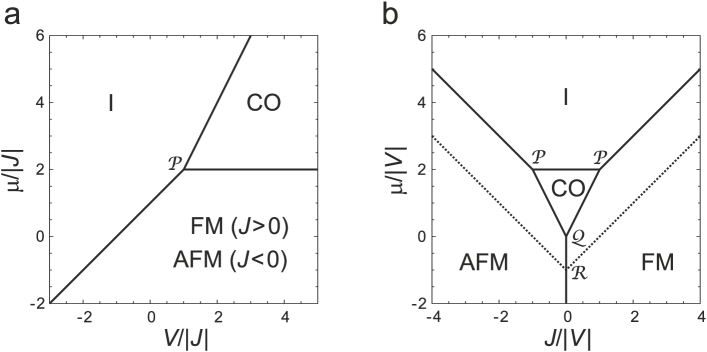
Figure 1: The phase diagrams of the 1D dilute Ising model (1) at zero temperature (a) in plane ($V/|J|$, $\mu/|J|$), (b) in plane ($J/|V|$, $\mu/|V|$). The impurity (I), charge-ordered (CO), ferromagnetic (FM), and antiferromagnetic (AFM) phases correspond to the following configurations of the $z$-components of the neighbour pseudospins: I $\rightarrow$ (0,0), CO $\rightarrow$ (0,$\pm 1$), FM $\rightarrow$ ($\pm 1$,$\pm 1$), AFM $\rightarrow$ ($1$,$-1$). (a) Solid lines are the coexistence curves of phases I, CO, and FM for $J>0$ or phases I, CO, and AFM for $J<0$. The point $\mathcal{P}$($V/|J|=1$ and $\mu/|J|=2$) is a tricritical point. (b) Solid lines show the coexistence curves of phases I, CO, FM, and AFM for $V>0$. Along with $\mathcal{P}$, the tricritical point $\mathcal{Q}$($J/|V|=0$ and $\mu/|V|=0$) is shown. Dashed lines show the coexistence curves of phases I and FM and phases I and AFM for $V<0$. In the latter case, the only tricritical point is $\mathcal{R}$($J/|V|=0$ and $\mu/|V|=-1$).

In Fig. 1 we present the phase diagrams of the 1D dilute Ising model (1) at zero temperature in planes ($V/|J|$, $\mu/|J|$) and ($J/|V|$, $\mu/|V|$). The impurity (I), charge-ordered (CO), ferromagnetic (FM), and antiferromagnetic (AFM) phases correspond to the following configurations of the $z$-components of the neighbour pseudospins: I $\rightarrow$ (0,0), CO $\rightarrow$ (0,1) or (0,$-1$), FM $\rightarrow$ (1,1) or ($-1$,$-1$), AFM $\rightarrow$ (1,$-1$). The values of the grand potential per one site at zero temperature for each phase are given by the expressions: $\omega_{I}=V-\mu$, $\omega_{CO}=-\mu/2$, $\omega_{FM}=-J$, $\omega_{AFM}=J$. This defines the concentration of impurities $n$ in each phase: $n_{I}=1$, $n_{CO}=1/2$, $n_{FM}=0$, $n_{AFM}=0$. Intermediate values of $n$ correspond to the states with phase separation, which are represented by the coexistence curves FM/CO and AFM/CO ($0<n<1/2$), CO/I ($1/2<n<1$), FM/I and AFM/I ($0<n<1$). The tricritical point $\mathcal{P}$ corresponds to the mixture of phases I, CO, and FM at $J>0$ (or I, CO, and AFM at $J<0$) when $V>0$ and $V=|J|$. The frustrated states for all $n$, $0<n<1$, arise because of the equal strength of the spin-spin and impurity-impurity interactions. The tricritical points $\mathcal{Q}$ and $\mathcal{R}$ represent completely disordered magnetic states since they correspond to the value $J=0$.

The qualitative difference of states at zero temperature is well illustrated by the entropy of the dilute Ising chain, defined as a function of temperature and impurities concentration by the following expression

$$s = {}-m\ln\left(2\,\frac{g+m}{g-m}\,e^{W}\cosh K\right)-{}$$ (29)

$${}-\frac{1}{2}\ln\frac{\frac{1}{4}-m^{2}}{2\left(g+\frac{1}{2}\right)^{2}}+\left(m+\frac{1}{2}\right)\frac{g+m}{g+\frac{1}{2}}\,W+{}$$

$$+\left(m-\frac{1}{2}\right)\frac{g-m}{g+\frac{1}{2}}\,K\tanh K.$$

The limiting values $s_{0}$ of entropy at $\theta=0$ are listed in Table 1 and are shown as a dependencies of the impurities concentration in Fig.2. We see that $s_{0}$ depends only on the concentration of impurities in different ways for $V<|J|$, $V=|J|$ and $V>|J|$, but does not depend on the interaction parameters themselves. If $V<|J|$, we get $s_{0}=0$, but if $V\geq|J|$, the entropy of the ground state is greater than zero, so these states should be referred to in modern language as frustrated Zarubin2019 . When $V=|J|$, the maximum value of entropy is $s_{0}=\ln\left(1+\sqrt{2}\right)\approx 0.881$ for $m=0$, while in the case $V>|J|$, the entropy has two maxima $s_{0}=\ln 2\approx 0.693$ at $|m|=\frac{1}{6}$ and the local minimum $s_{0}=\frac{1}{2}\ln 2\approx 0.347$ at $m=0$.

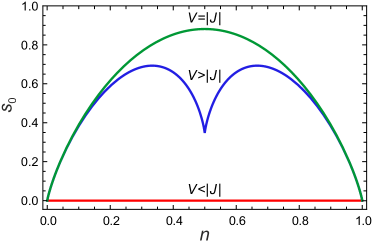
Figure 2: (color online) An entropy of the 1D dilute Ising model at zero temperature for $V<|J|$, $V=|J|$ and $V>|J|$.

Parameters	$s_{0}$
$V<|J|$	$0$
$V=|J|$	$\displaystyle\ln\left(\frac{1}{2}+g_{0}\right)+\frac{1}{2}\ln\frac{2}{\frac{1}{4}-m^{2}}-m\ln\frac{g_{0}+m}{g_{0}-m}$
$V>|J|$	$\displaystyle\frac{1}{2}\ln\frac{1+2|m|}{1-2|m|}+|m|\ln\frac{\frac{1}{4}-m^{2}}{8m^{2}}+\frac{1}{2}\ln 2$

Table 1: The zero-temperature value $s_{0}$ of entropy defined by equation (29) for different sets of parameters of the dilute Ising chain.

Parameters	$\displaystyle\ell$	$\displaystyle\ell_{0}$
$V<|J|$	$\displaystyle\propto e^{\frac{|K|-W}{2}}$	$\displaystyle\propto e^{\frac{|K|-W}{2}}$
$V=|J|$	$\displaystyle\left(\ln\frac{g_{0}+\frac{1}{2}}{g_{0}-m}\right)^{\!\!-1}$	$\displaystyle\left(\ln\frac{1+2g_{0}}{1-2g_{0}}\right)^{\!\!-1}$
$V>|J|$ $m<0$	$\displaystyle\left(\ln\frac{|m|+\frac{1}{2}}{2|m|}\right)^{\!\!-1}$	$\displaystyle\left(\ln\frac{1+2|m|}{1-2|m|}\right)^{\!\!-1}$
$V>|J|$ $m=0$	$0$	$\displaystyle\propto e^{\frac{W-|K|}{2}}$
$V>|J|$ $m>0$	$0$	$\displaystyle\left(\ln\frac{1+2|m|}{1-2|m|}\right)^{\!\!-1}$

Table 2: Asymptotic behavior of the spin correlation length $\ell$ and the impurity correlation length $\ell_{0}$ at zero temperature for different sets of parameters.

Concentration dependences of the spin correlation length and the impurity correlation length at low temperature ($\theta/|J|=0.1$) are shown in Fig.3 for certain values of $V/|J|$. The analytical expressions of the low-temperature asymptotics of $\ell$ and $\ell_{0}$ are presented in Table 2. The parameter $g_{0}$ is given by

$$g_{0}=\frac{1}{\sqrt{2}}\left(\frac{1}{4}+m^{2}\right)^{1/2}.$$ (30)

Like other thermodynamic properties of the dilute Ising chain, the low-temperature limits of $\ell$ and $\ell_{0}$ are qualitatively different for $V<|J|$, $V=|J|$, and $V>|J|$. If $V<|J|$, both $\ell$, and $\ell_{0}$ tend to infinity with the same asymptotic behavior. This means that with decreasing temperature the system is divided into macroscopically homogeneous domains consisting of non-magnetic impurities and magnetic sites, respectively. In this case, the magnetic matrix pushes impurities, thereby minimizing the surface energy. Another quasi-ordered situation appears at $V>|J|$ and $m=0$ ($n=1/2$), when the impurity correlation length tends to infinity in contrast to the spin correlation length which tends to zero. This indicates the formation of charge ordering at zero temperature when the sites occupied by non-magnetic charged impurities with $\sigma=0$ alternate with the sites occupied by the spin states with $\sigma=\pm 1$. Due to the short-range character of the exchange interaction, the spin subsystem becomes an ideal paramagnet.

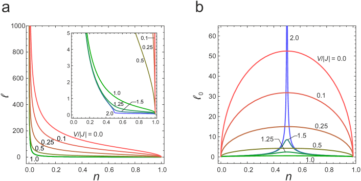
Figure 3: (color online) Concentration dependences of (a) the spin correlation length $\ell$ and (b) the impurity correlation length $\ell_{0}$ at $\theta/|J|=0.1$ for different values of $V/|J|$. The insert in (a) shows that the spin correlation length tends to zero at low temperatures for $V>|J|$ and $n\geq 0.5$.

An analysis of the correlation lengths makes it interesting to study sequences of ferromagnetically ordered spins with $\boldsymbol{\sigma}=(\pm)$, antiferromagnetic sequences with $\boldsymbol{\sigma}=({+}{-})$, sequences of impurities with $\boldsymbol{\sigma}=(0)$, and charge-ordered sequences with $\boldsymbol{\sigma}=(01)$. We give the expressions of the parameter $q_{\boldsymbol{\sigma}}$ in the geometric distribution (27) for these sequences in Table 3.

$\boldsymbol{\sigma}$	$(0)$	$({\pm})$	$({+}{-})$	$(01)$
$q_{\boldsymbol{\sigma}}$	$\displaystyle\frac{g{+}m}{g{+}\frac{1}{2}}$	$\displaystyle\frac{(g{-}m)e^{K}}{\left(2g{+}1\right)\cosh K}$	$\displaystyle\frac{(g{-}m)^{2}e^{-2K}}{\left(2g{+}1\right)^{\!2}\!\cosh^{2}\!K}$	$\displaystyle\frac{\frac{1}{4}{-}m^{2}}{\left(g{+}\frac{1}{2}\right)^{\!2}}$

Table 3: The parameter $q_{\boldsymbol{\sigma}}$ of geometric distribution (27) for sequences of repeating blocks $\boldsymbol{\sigma}$.

The low-temperature properties of the mean lengths of repeating sequences are listed in Table 4.

If $V<|J|$, the mean length of the impurity sequences $\bar{l}_{(0)}$ diverges at $\theta\to 0$, having the same asymptotic behavior as the impurity correlation length $\ell_{0}$. If $V\geq|J|$, $\bar{l}_{(0)}$ remains finite at zero temperature, and if $m\leq 0$, the mean length approaches its minimum value, $\bar{l}_{(0)}=1$, that corresponds to single impurities separated by the chain sites with $\sigma=\pm 1$.

Parameters	$\displaystyle\bar{l}_{(0)}$	$\displaystyle\bar{l}_{(\pm)}$	$\displaystyle\bar{l}_{(01)}$
$V<|J|$	$\displaystyle\propto e^{\frac{|K|-W}{2}}$	$\displaystyle\propto e^{\frac{|K|-W}{2}}$	$1$
$V=|J|$	$\displaystyle\frac{2g_{0}+1}{1-2m}$	$\displaystyle\frac{2g_{0}+1}{1+2m}$	$\displaystyle\frac{g_{0}^{2}+g_{0}+\frac{1}{4}}{g_{0}^{2}+g_{0}+m^{2}}$
$V>|J|$ $m\neq 0$	$\displaystyle\frac{1+2|m|}{1-2m}$	$\displaystyle\frac{1+2|m|}{1+2m}$	$\displaystyle\frac{\frac{1}{2}+|m|}{2|m|}$
$V>|J|$ $m=0$	$1$	$1$	$\displaystyle\propto e^{\frac{W-|K|}{2}}$

Table 4: Asymptotic behavior of the mean lengths for the impurity sequences $(0)^{l}$, ferromagnetic sequences $(\pm)^{l}$ and the charge-ordered sequences $(01)^{l}$ at zero temperature.

Asymptotic behavior of $\bar{l}_{(\pm)}$ and $\bar{l}_{({+}{-})}$ at $\theta\to 0$ depends on the sign of $J$. If $J<0$ ($J>0$), we obtain $\bar{l}_{(\pm)}=1$ ($\bar{l}_{({+}{-})}=1$) at $\theta=0$ for any parameters of the dilute Ising chain. If $J>0$, asymptotic expressions for ferromagnetic sequences and for the impurity sequences differ by replacing $m$ with $-m$. The value of $\bar{l}_{(\pm)}$ diverges for $V<|J|$ and has the same asymptotic behavior as the spin correlation length $\ell$. If $V\geq|J|$, $\bar{l}_{(\pm)}$ remains finite at zero temperature, and if $m\geq 0$, we obtain $\bar{l}_{(\pm)}=1$. If $J<0$, asymptotic behavior of $\bar{l}_{({+}{-})}$ is the same as of $\bar{l}_{(\pm)}$ for $J>0$ with some difference in amplitude due to the number of sites in the minimum block of ferromagnetic and antiferromagnetic sequences.

The low-temperature limit of $\bar{l}_{(01)}$ at $V<|J|$ complements the previous results for the impurity and spin sequences since the pair $(01)$ is just the boundary between them. The concentration of pairs $(01)$

$$\left\langle P_{0,k}P_{1,k+1}\right\rangle=P(01)=\frac{\frac{1}{2}-2m^{2}}{2g+1}$$ (31)

becomes zero only at $\theta=0$, which corresponds to the infinity length of the impurity and the spin sequences. If $V=|J|$ or $V>|J|$, $m\neq 0$, $\bar{l}_{(01)}$ is finite, and only if $V>|J|$ and $m=0$, the mean length for the charge ordered sequences tends to infinity at $\theta\to 0$. The asymptotic behavior of $\bar{l}_{(01)}$ determines the asymptotic behavior of the impurity correlation length $\ell_{0}$ in this case.

The results found in this section specify details of the ordering processes in the dilute Ising chain with decreasing temperature. For repeating sequences $\boldsymbol{\sigma}^{l}$, the geometric distribution $p_{l}$ of lengths $l$ realizes, $p_{l}=(1-q_{\boldsymbol{\sigma}})q_{\boldsymbol{\sigma}}^{l-1}$. The mean length $\bar{l}_{\boldsymbol{\sigma}}=(1-q_{\boldsymbol{\sigma}})^{-1}$ tends to infinity only if $q_{\boldsymbol{\sigma}}$ goes to unity, and the dispersion of the cluster lengths also tends to infinity, asymptotically as a square of $\bar{l}_{\boldsymbol{\sigma}}$: $D(l_{\boldsymbol{\sigma}})=q_{\boldsymbol{\sigma}}(1-q_{\boldsymbol{\sigma}})^{-2}\propto\bar{l}_{\boldsymbol{\sigma}}^{2}$. The final ordering at zero temperature is achieved only when the concentration of the boundaries of the sequences becomes zero. This is similar to the well-known result of the percolation theory, where the site percolation threshold in the 1D problem equals unity.

It is worth noting that both at $V<|J|$ and at $V>|J|$, the specific heat of the dilute Ising chain has the low-temperature peak that can be directly related to the concentration of the impurity–spin pairs, $\left\langle P_{0,k}P_{1,k+1}\right\rangle$. The internal energy can be written using PDF in the form:

$$\varepsilon=-J\left\langle P_{1,k}P_{1,k+1}\right\rangle\tanh K+V\left\langle P_{0,k}P_{0,k+1}\right\rangle,$$ (32)

where we use the relation $\left\langle\sigma_{k}\sigma_{k+1}\right\rangle=\left\langle P_{1,k}P_{1,k+1}\right\rangle\tanh K$. Differentiating by temperature the identity $\left\langle P_{0,k}P_{0,k+1}\right\rangle+\left\langle P_{1,k}P_{1,k+1}\right\rangle+2\left\langle P_{0,k}P_{1,k+1}\right\rangle=1$ we find

$$\left\langle P_{0,k}P_{0,k+1}\right\rangle_{\theta}^{\prime}=\left\langle P_{1,k}P_{1,k+1}\right\rangle_{\theta}^{\prime}=-\left\langle P_{0,k}P_{1,k+1}\right\rangle_{\theta}^{\prime}.$$ (33)

The first equality in (33) can be obtained from equations (6) and (13). Hence the specific heat takes the form

$$c = \left\langle P_{0,k}P_{1,k+1}\right\rangle_{\theta}^{\prime}\left(J\tanh K-V\right)+{}$$ (34)

$${}+\left\langle P_{1,k}P_{1,k+1}\right\rangle\frac{K^{2}}{\cosh^{2}K}.$$

The contribution to the specific heat of the first and second terms in (34) is shown in Fig.4a,b. The expression for the specific heat of the pure Ising chain arises from the second term. We see, that the low-temperature peak for $n\neq 0$ is mainly determined by the maximum rate of change with the temperature of the concentration of the impurity–spin pairs. Using the low-temperature asymptotics, we can obtain a simple estimation for the specific heat maximum due to the impurities ordering at $V<|J|$ and at $V>|J|$, $m=0$:

$$\theta_{0}=\frac{\left||J|-V\right|}{4}.$$ (35)

As is known, the correlation length determines the characteristic spatial scale of the system near the critical point. Indeed, at $\theta=0$, the asymptotics of the spin correlation length $\ell$ coincides with the asymptotics of $\bar{l}_{(\pm)}$ at $J>0$ or $\bar{l}_{({+}{-})}$ at $J<0$ for $V<|J|$. Also the asymptotics of the impurity correlation length $\ell_{0}$ coincides with the asymptotics of $\bar{l}_{(0)}$ for $V<|J|$ or $\bar{l}_{(01)}$ for $V>|J|$. But, as shown in Fig.4c,d, the peak of the specific heat corresponds to small values of the correlation lengths and is not associated with any features of the temperature dependences of $\ell$ and $\ell_{0}$. However, this peak can be associated with the mean length of the impurity sequences $\bar{l}_{(0)}$, as $1/\bar{l}_{(0)}$ is proportional to the concentration of the impurity–spin pairs:

$$\frac{1}{\bar{l}_{(0)}}=\frac{2}{1+2m}\left\langle P_{0,k}P_{1,k+1}\right\rangle.$$ (36)

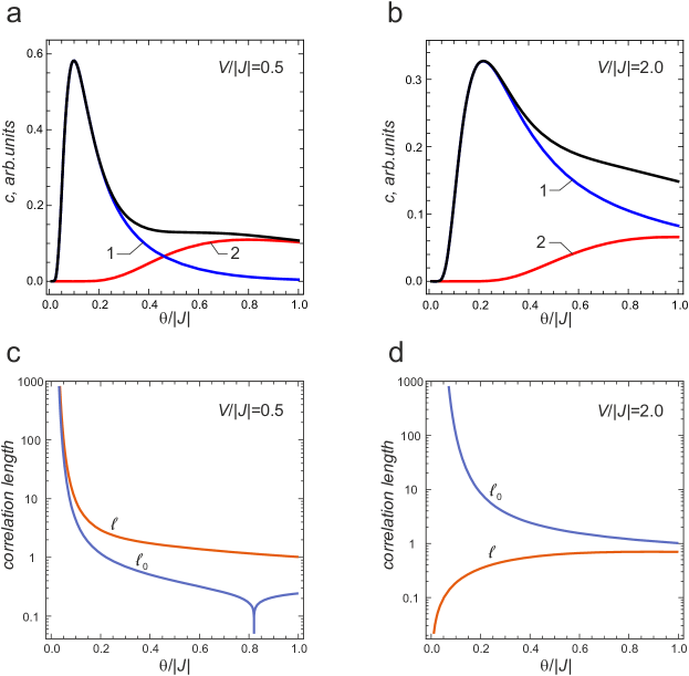
Figure 4: (color online) Specific heat and the contributions of first (– 1) and second (– 2) terms in equation (34) for $m=0$ ($n=1/2$) (a) at $V/|J|=0.5$ and (b) at $V/|J|=2.0$. The spin correlation length $\ell$ and the impurity correlation length $\ell_{0}$ for $m=0$ (c) at $V/|J|=0.5$ and (d) at $V/|J|=2.0$. The $y$-axis in (c) and (d) has a logarithmic scale. The peculiarity of $\ell_{0}$ near $\theta/|J|=0.8$ in (c) corresponds to the solution of the equation $\Lambda_{0}=0$ discussed at the end of Section 16.

It is also worth to note that there are no other repeating sequences $\boldsymbol{\sigma}^{l}$, except for previously discussed, for which the mean length $\bar{l}_{\boldsymbol{\sigma}}$ tends to infinity at zero temperature. This is a consequence of properties of the conditional probability functions defined by matrices (18) and (20). Their limiting values at zero temperature are given in Table 5. The parameter $q_{\boldsymbol{\sigma}}$ in the geometric distribution $p_{l}$ is the probability of the cycle $\boldsymbol{\sigma}$, which is defined by the finite product of conditional probabilities (23). As can be seen from Table 5, the cycles different from the impurities, from the spins, ordered ferromagnetically at $J>0$, from the spins, ordered anti-ferromagnetically at $J<0$, or from the impurity–spin pairs, have the value of $q_{\boldsymbol{\sigma}}$ less than unity at $\theta=0$, which gives a finite value of $\bar{l}_{\boldsymbol{\sigma}}=(1-q_{\boldsymbol{\sigma}})^{-1}$ at zero temperature.

In conclusion, we list briefly the main properties of Markov chains generated by the matrices in Table 5. If $V<|J|$, the Markov chains are reducible. For $K>0$, three classes correspond to states with $\sigma={+}1,\,0,\,{-}1$. For $K<0$, the states with $\sigma=\pm 1$ form a periodic class that indicates antiferromagnetic ordering. In a Markov chain with a transition matrix $\mathcal{P}^{\prime T}$ the states with $\sigma=\pm 1$ are considered as one magnetic state, therefore, this Markov chain has 2 classes consisting of the impurity and magnetic states. If $V=|J|$, all Markov chains are irreducible and aperiodic, i.e., regular. If $V>|J|$ and $m\neq 0$, the Markov chains are also irreducible and aperiodic, but when $m=0$, the Markov chains becomes periodic. Two classes of states, one of which consists of an impurity state and the other consists of magnetic states, have a period 2. In all cases, the considered Markov chains do not have transient states, but, obviously, in an external longitudinal magnetic field, one magnetic state will become transient.

As a result, the non-ordered dilute Ising chain is described by the regular Markov chain, while the ordering generates the irregular Markov chain. The phase separation at $V<|J|$ generates the reducible Markov chain, and the charge ordering at $V>|J|$, $m=0$ generates the periodic one, which reflects the qualitative difference between these cases.

	$\mathcal{P}$		$\mathcal{P}^{\prime}$
​​Parameters	$K>0$	$K<0$
​​ $V{<}|J|$	$\begin{pmatrix}1&0&0\\ 0&~{}1~{}&0\\ 0&0&1\end{pmatrix}$	$\begin{pmatrix}0&0&1\\ 0&~{}1~{}&0\\ 1&0&0\end{pmatrix}$	$\begin{pmatrix}1&~{}0\\ 0&~{}1\end{pmatrix}$
​​ $V{=}|J|$	$\begin{pmatrix}1{-}a&\frac{b}{2}&0\\ a&1{-}b&a\\ 0&\frac{b}{2}&1{-}a\end{pmatrix}$	$\begin{pmatrix}0&\frac{b}{2}&1{-}a\\ a&1{-}b&a\\ 1{-}a&\frac{b}{2}&0\end{pmatrix}$	$\begin{pmatrix}1{-}b&a\\ b&1{-}a\end{pmatrix}$
​​ $V{>}|J|$ $m{<}0$	$\begin{pmatrix}1{-}c&\frac{1}{2}&0\\ c&~{}0~{}&c\\ 0&\frac{1}{2}&1{-}c\end{pmatrix}$	$\begin{pmatrix}0&\frac{1}{2}&1{-}c\\ c&~{}0~{}&c\\ 1{-}c&\frac{1}{2}&0\end{pmatrix}$	$\begin{pmatrix}0~{}&c\\ 1~{}&1{-}c\end{pmatrix}$
​​ $V{>}|J|$ $m{=}0$	$\begin{pmatrix}0&\frac{1}{2}&0\\ 1&~{}0~{}&1\\ 0&\frac{1}{2}&0\end{pmatrix}$	$\begin{pmatrix}0&\frac{1}{2}&0\\ 1&~{}0~{}&1\\ 0&\frac{1}{2}&0\end{pmatrix}$	$\begin{pmatrix}0&~{}1\\ 1&~{}0\end{pmatrix}$
​​ $V{>}|J|$ $m{>}0$	$\begin{pmatrix}0&\frac{c}{2}&0\\ 1&~{}1{-}c~{}&1\\ 0&\frac{c}{2}&0\end{pmatrix}$	$\begin{pmatrix}0&\frac{c}{2}&0\\ 1&~{}1{-}c~{}&1\\ 0&\frac{c}{2}&0\end{pmatrix}$	$\begin{pmatrix}1{-}c&~{}1\\ c&~{}0\end{pmatrix}$

Table 5: The zero temperature values of the conditional probability matrices $\mathcal{P}$ and $\mathcal{P}^{\prime}$. Here $a=\left(1+2m\right)/\left(1+2g_{0}\right)$, $b=\left(1-2m\right)/\left(1+2g_{0}\right)$, $c=\left(1-2|m|\right)/\left(1+2|m|\right)$, and the expression of $g_{0}$ is defined by equation (30).

IV Conclusion

We examined pair distribution functions and local distributions for the 1D dilute Ising model. The thermodynamic properties of the Ising chain with impurities qualitatively differ from the case of a pure Ising chain and depend on the ratio of the exchange constant ($J$) and the impurities interaction parameter ($V$). An analysis shows that if $V<|J|$, the phase separation occurs when the system is divided into macroscopic domains consisting only of impurities or only of spins. In this case, both the spin and impurity correlation lengths diverge at zero temperature. If $V\geq|J|$, the system is frustrated and its entropy does not equal zero at zero temperature. While the spin correlation length is always finite, the impurity correlation length tends to infinity at half-filling and $V>|J|$. If $V\neq|J|$, the specific heat of the dilute Ising chain has a distinct maximum at some critical temperature due to the ordering processes in the impurities subsystem. We found that this critical temperature is determined by the maximum rate of change of the impurity–spin pairs concentration and is proportional to the modulus of a difference between the exchange constant and the impurities interaction parameter. Unlike the dilute Ising chain, in the two-dimensional dilute Ising system with mobile impurities and in related models Arora1973 ; Wortis1974b ; Yaldram1993 ; Khalil1997 ; Loois2008 ; Panov2019 , the previously considered orderings are the phase transitions at finite temperatures. If $V<|J|$ and the impurities concentration $n<n_{c}$, the spin ordering with the temperature lowering precedes to the phase separation when the domains containing only impurities or only spin centers occur. If $n>n_{c}$, the phase separation appears simultaneously with the spin ordering in the spin domains. If $V>|J|$, the diluted spin ordering at $n<n^{\prime}_{c}$ is changed at $n>n^{\prime}_{c}$ by the charge ordering of impurities with the short-range spin order.

To consider the details of the ordering processes, we explored the local distributions. The Markov property of the dilute Ising chain allowed us to use the conditional probabilities for the nearest neighbors to obtain the expressions of the pair distribution functions, the probability of any finite sequence and, in particular, of an isolated sequence of repeating blocks. The lengths of isolated sequences of repeating blocks $\boldsymbol{\sigma}$ obey the geometric distribution, and the probability of the cycle $\boldsymbol{\sigma}$ is the only parameter determining its properties. If the mean length of some repeating sequence tends to infinity, the dispersion of lengths also tends to infinity, asymptotically as a square of the mean length. We showed that the critical behavior of the spin correlation length at $V<|J|$ is defined by ferromagnetic sequences for $J>0$ and by antiferromagnetic sequences for $J<0$, while the critical behavior of the impurity correlation length is defined by the sequences of impurities at $V<|J|$ and by the charge-ordered sequences at half-filling and $V>|J|$. We concluded that for the dilute Ising chain there are no other repeating sequences for which the mean length tends to infinity at zero temperature. We found that the non-ordered dilute Ising chain corresponds to the regular Markov chain, while the ordering generates the irregular Markov chain.

References

- (1) F. Y. Wu, Phase Diagram of a Spin-One Ising System, Chinese Journal of Physics 16 (2) (1978) 153–156.
- (2) M. Thomaz, E. Corrêa Silva, Comparison of the ferromagnetic Blume–Emery–Griffiths model and the AF spin-1 longitudinal Ising model at low temperature, Journal of Magnetism and Magnetic Materials 401 (2016) 633–646. doi:10.1016/j.jmmm.2015.10.071.
- (3) E. Corrêa Silva, M. Thomaz, Comparison of the exact thermodynamics of the AF Blume–Emery–Grifiths and of the spin-1 ferromagnetic Ising models, Journal of Magnetism and Magnetic Materials 417 (2016) 365–375. doi:10.1016/j.jmmm.2016.05.039.
- (4) M. S. S. Pereira, F. A. B. F. de Moura, M. L. Lyra, Magnetization plateau in diamond chains with delocalized interstitial spins, Physical Review B 77 (2) (2008) 024402. doi:10.1103/PhysRevB.77.024402.
- (5) Z. Yang, L. Yang, J. Dai, T. Xiang, Rigorous Solution of the Spin-1 Quantum Ising Model with Single-Ion Anisotropy, Physical Review Letters 100 (6) (2008) 067203. doi:10.1103/PhysRevLett.100.067203.
- (6) Z.-H. Yang, L.-P. Yang, H.-N. Wu, J. Dai, T. Xiang, Exact solutions of a class of S=1 quantum Ising spin models, Physical Review B 79 (21) (2009) 214427. doi:10.1103/PhysRevB.79.214427.
- (7) S. de Souza, M. Thomaz, The magnetization plateaus of the ferro and anti-ferro spin-1 classical models with Sz2 term, Journal of Magnetism and Magnetic Materials 354 (2014) 205–215. doi:10.1016/j.jmmm.2013.10.041.
- (8) H. Wu, G. Wei, P. Zhang, G. Yi, W. Gong, Thermodynamic properties of the mixed spin-1/2 and spin-1 Ising chain with both longitudinal and transverse single-ion anisotropies, Journal of Magnetism and Magnetic Materials 322 (21) (2010) 3502–3507. doi:10.1016/j.jmmm.2010.06.053.
- (9) H. Wu, G. Wei, A. Du, G. Yi, W. Gong, Exact results of an alternating-bond mixed spin-1/2 and spin-1 Ising chain with both longitudinal and transverse single-ion anisotropies, Journal of Magnetism and Magnetic Materials 323 (11) (2011) 1428–1432. doi:10.1016/j.jmmm.2010.12.027.
- (10) J. Strečka, M. Dančo, Unusual field-induced transitions in exactly solved mixed spin-(1/2, 1) Ising chain with axial and rhombic zero-field splitting parameters, Physica B: Condensed Matter 406 (15-16) (2011) 2967–2976. doi:10.1016/j.physb.2011.04.040.
- (11) L. Čanová, J. Strečka, M. Jaščur, Geometric frustration in the class of exactly solvable Ising–Heisenberg diamond chains, Journal of Physics: Condensed Matter 18 (20) (2006) 4967–4984. doi:10.1088/0953-8984/18/20/020.
- (12) D. Antonosyan, S. Bellucci, V. Ohanyan, Exactly solvable Ising-Heisenberg chain with triangular XXZ -Heisenberg plaquettes, Physical Review B 79 (1) (2009) 014432. doi:10.1103/PhysRevB.79.014432.
- (13) O. Rojas, S. M. de Souza, V. Ohanyan, M. Khurshudyan, Exactly solvable mixed-spin Ising-Heisenberg diamond chain with biquadratic interactions and single-ion anisotropy, Physical Review B 83 (9) (2011) 094430. doi:10.1103/PhysRevB.83.094430.
- (14) L. Gálisová, Magnetic properties of the spin-1/2 Ising-Heisenberg diamond chain with the four-spin interaction, physica status solidi (b) 250 (1) (2013) 187–195. doi:10.1002/pssb.201248260.
- (15) J. Torrico, M. Rojas, S. M. de Souza, O. Rojas, N. S. Ananikian, Pairwise thermal entanglement in the Ising-XYZ diamond chain structure in an external magnetic field, EPL (Europhysics Letters) 108 (5) (2014) 50007. doi:10.1209/0295-5075/108/50007.
- (16) B. Lisnyi, J. Strečka, Exactly solved mixed spin-(1,1/2) Ising–Heisenberg diamond chain with a single-ion anisotropy, Journal of Magnetism and Magnetic Materials 377 (2015) 502–510. doi:10.1016/j.jmmm.2014.10.113.
- (17) L. Gálisová, J. Strečka, Vigorous thermal excitations in a double-tetrahedral chain of localized Ising spins and mobile electrons mimic a temperature-driven first-order phase transition, Physical Review E 91 (2) (2015) 022134. doi:10.1103/PhysRevE.91.022134.
- (18) O. Rojas, J. Strečka, S. de Souza, Thermal entanglement and sharp specific-heat peak in an exactly solved spin-1/2 Ising-Heisenberg ladder with alternating Ising and Heisenberg inter–leg couplings, Solid State Communications 246 (2016) 68–75. doi:10.1016/j.ssc.2016.08.002.
- (19) J. Strečka, R. C. Alécio, M. L. Lyra, O. Rojas, Spin frustration of a spin-1/2 Ising–Heisenberg three-leg tube as an indispensable ground for thermal entanglement, Journal of Magnetism and Magnetic Materials 409 (2016) 124–133. doi:10.1016/j.jmmm.2016.02.095.
- (20) J. Torrico, J. Strečka, M. Hagiwara, O. Rojas, S. de Souza, Y. Han, Z. Honda, M. Lyra, Heterobimetallic Dy-Cu coordination compound as a classical-quantum ferrimagnetic chain of regularly alternating Ising and Heisenberg spins, Journal of Magnetism and Magnetic Materials 460 (2018) 368–380. doi:10.1016/j.jmmm.2018.04.021.
- (21) B. M. Lisnii, Distorted diamond Ising-Hubbard chain, Low Temperature Physics 37 (4) (2011) 296–304. doi:10.1063/1.3592221.
- (22) H. S. Sousa, M. S. S. Pereira, I. N. de Oliveira, J. Strečka, M. L. Lyra, Phase diagram and re-entrant fermionic entanglement in a hybrid Ising-Hubbard ladder, Physical Review E 97 (5) (2018) 052115. doi:10.1103/PhysRevE.97.052115.
- (23) S. de Souza, O. Rojas, Quasi-phases and pseudo-transitions in one-dimensional models with nearest neighbor interactions, Solid State Communications 269 (2018) 131–134. doi:10.1016/j.ssc.2017.10.006.
- (24) M. Suzuki, B. Tsujiyama, S. Katsura, One-Dimensional Ising Model with General Spin, Journal of Mathematical Physics 8 (1) (1967) 124. doi:10.1063/1.1705089.
- (25) S. Muto, T. Oguchi, One-Dimensional Random Annealed Ising Spin System on the Site Model, Progress of Theoretical Physics 56 (6) (1976) 1669–1673. doi:10.1143/PTP.56.1669.
- (26) S. B. Haley, II. Exact solutions of disordered Ising spin chains in a magnetic field, Journal of Mathematical Physics 19 (5) (1978) 1187–1191. doi:10.1063/1.523782.
- (27) L. Gonçalves, A. Vieira, Ising chain with random short- and long-range interactions, Journal of Magnetism and Magnetic Materials 177-181 (1998) 76–78. doi:10.1016/S0304-8853(97)00306-5.
- (28) H. Fakhri, S. Seyedein Ardebili, Exact solutions for the ferromagnetic and antiferromagnetic two-ring Ising chains of spin-1/2, Physica A: Statistical Mechanics and its Applications 523 (2019) 557–569. doi:10.1016/j.physa.2019.02.004.
- (29) F. A. Kassan-ogly, One-dimensional ising model with next-nearest-neighbour interaction in magnetic field, Phase Transitions 74 (4) (2001) 353–365. doi:10.1080/01411590108227581.
- (30) A. I. Proshkin, T. Y. Ponomareva, I. A. Menshikh, A. V. Zarubin, F. A. Kassan-Ogly, Correlation function of one-dimensional s = 1 Ising model, Physics of Metals and Metallography 118 (10) (2017) 929–934. doi:10.1134/S0031918X17100106.
- (31) A. V. Zarubin, F. A. Kassan-Ogly, A. I. Proshkin, A. E. Shestakov, Frustration Properties of the 1D Ising Model, Journal of Experimental and Theoretical Physics 128 (5) (2019) 778–807. doi:10.1134/S106377611904006X.
- (32) S. Katsura, B. Tsujiyama, Ferro- and Antiferromagnetism of Dilute Ising Model, in: C. Domb (Ed.), Proceedings of the Conference on PhenomenaPhenomena in the Neighborhood of Critical Points, National Bureau of Standards, Washington, D.C., 1965, pp. 219–224.
- (33) M. P. Kawatra, L. J. Kijewski, Exact Solution of a One-Dimensional Magnetic Lattice Gas with an Ising Interaction, Physical Review 183 (1) (1969) 291–294. doi:10.1103/PhysRev.183.291.
- (34) F. Rys, A. Hintermann, Gittermodell eines ungeordneten Ferromagneten II. Exakte Losung des eindimensionalen Dodells, Helv. Phys. Acta 42 (4) (1969) 608.
- (35) F. Matsubara, K. Yoshimura, S. Katsura, Magnetic Properties of One-Dimensional Dilute Ising Systems. I, Canadian Journal of Physics 51 (10) (1973) 1053–1063. doi:10.1139/p73-140.
- (36) Y. Termonia, J. Deltour, Thermodynamic properties of one-dimensional dilute Ising systems with interacting impurities, Journal of Physics C: Solid State Physics 7 (24) (1974) 4441–4451. doi:10.1088/0022-3719/7/24/007.
- (37) B. Balagurov, V. Vaks, R. Zaitsev, Statistics of a One-Dimensional Model of a Solid Solution, Sov Phys Solid State 16 (8) (1974) 1498–1502.
- (38) M. Wortis, Griffiths singularities in the randomly dilute one-dimensional Ising model, Physical Review B 10 (11) (1974) 4665–4671. doi:10.1103/PhysRevB.10.4665.
- (39) V. G. Vaks, N. E. Zein, Theory of phase transitions in solid solutions, JETP 40 (3) (1975) 537.
- (40) A. B. Harris, Nature of the ”Griffiths” singularity in dilute magnets, Physical Review B 12 (1) (1975) 203–207. doi:10.1103/PhysRevB.12.203.
- (41) K. Binder, “Clusters” in the Ising model, metastable states and essential singularity, Annals of Physics 98 (2) (1976) 390–417. doi:10.1016/0003-4916(76)90159-7.
- (42) J. Marro, R. Toral, Equilibrium cluster distributions of the three-dimensional Ising model in the one phase region, Physica A: Statistical Mechanics and its Applications 122 (3) (1983) 563–586. doi:10.1016/0378-4371(83)90049-3.
- (43) M. Thomsen, M. F. Thorpe, Dilute Ising chains with spin S, Journal of Physics C: Solid State Physics 16 (21) (1983) 4191–4198. doi:10.1088/0022-3719/16/21/020.
- (44) R. Toral, C. Wall, Finite-size scaling study of the equilibrium cluster distribution of the two-dimensional Ising model, Journal of Physics A: Mathematical and General 20 (14) (1987) 4949–4965. doi:10.1088/0305-4470/20/14/032.
- (45) C.-K. Hu, Cluster-size distribution and the magnetic property of a potts model, Physical Review B 34 (9) (1986) 6280–6287. doi:10.1103/PhysRevB.34.6280.
- (46) R. Kühn, Thermally correlated frozen-in disorder in a linear magnetic chain, Zeitschrift für Physik B Condensed Matter 66 (2) (1987) 167–173. doi:10.1007/BF01311652.
- (47) J. Vavro, Exact solution for the lattice gas model in one dimension, Physical Review E 63 (5) (2001) 057104. doi:10.1103/PhysRevE.63.057104.
- (48) X. Campi, H. Krivine, J. Krivine, Clustering and thermodynamics in the lattice-gas model, Physica A: Statistical Mechanics and its Applications 320 (2003) 41–50. doi:10.1016/S0378-4371(02)01514-5.
- (49) M. B. Yilmaz, F. M. Zimmermann, Exact cluster size distribution in the one-dimensional Ising model, Physical Review E 71 (2) (2005) 026127. doi:10.1103/PhysRevE.71.026127.
- (50) J.-P. Simonin, Local Composition in a Binary Mixture on a One-Dimensional Ising Lattice, Industrial & Engineering Chemistry Research 52 (27) (2013) 9497–9504. doi:10.1021/ie4014138.
- (51) V. A. Malyshev, R. A. Minlos, Gibbs Random Fields, Springer Netherlands, 1991. doi:10.1007/978-94-011-3708-9.
- (52) B. L. Arora, D. P. Landau, H. C. Wolfe, C. D. Graham, J. J. Rhyne, Monte Carlo Studies of Tricritical Phenomena, in: AIP Conference Proceedings, Vol. 10, AIP, 1973, pp. 870–874. doi:10.1063/1.2947039.
- (53) M. Wortis, Tricritical behavior in the dilute Ising ferromagnet, Physics Letters A 47 (6) (1974) 445–446. doi:10.1016/0375-9601(74)90569-6.
- (54) K. Yaldram, G. Khalil, A. Sadiq, Phase diagram of a dilute binary alloy with annealed vacancies, Solid State Communications 87 (11) (1993) 1045–1049. doi:10.1016/0038-1098(93)90558-5.
- (55) G. K. Khalil, K. Yaldram, A. Sadiq, Phase Diagram of a Two-Dimensional Dilute Binary Alloy, International Journal of Modern Physics C 08 (02) (1997) 139–146. doi:10.1142/S012918319700014X.
- (56) C. C. Loois, G. T. Barkema, C. M. Smith, Monte Carlo studies of extensions of the Blume-Emery-Griffiths model, Physical Review B 78 (18) (2008) 184519. doi:10.1103/PhysRevB.78.184519.
- (57) Y. Panov, V. Ulitko, K. Budrin, A. Chikov, A. Moskvin, Phase diagrams of a 2D Ising spin-pseudospin model, Journal of Magnetism and Magnetic Materials 477 (2019) 162–166. doi:10.1016/j.jmmm.2019.01.049.