Magnetization generated by microwave-induced Rashba interaction

Abstract

We show that a controllable dc magnetization is accumulated in a junction comprising a quantum dot coupled to non-magnetic reservoirs if the junction is subjected to a time-dependent spin-orbit interaction. The latter is induced by an ac electric field generated by microwave irradiation of the gated junction. The magnetization is caused by inelastic spin-flip scattering of electrons that tunnel through the junction, and depends on the polarization of the electric field: a circularly polarized field leads to the maximal effect, while there is no effect in a linearly polarized field. Furthermore, the magnetization increases as a step function (smoothened by temperature) as the microwave photon energy becomes larger than the absolute value of the difference between the single energy level on the quantum dot and the common chemical potential in the leads.

I Introduction

The possibility to create and manipulate magnetic order confined to the nanometer length scale is currently attracting interest because of possible implications for magnetic devices and material developments Sander . Such a confined magnetization is seldom achieved by applying an external magnetic field, due to practical difficulties encountered when attempting to spatially localize the field. It can, however, be realized by modulating the exchange-interaction strength, for instance along a depth-profile variation of certain alloys’ constituents Kirby . In contrast to external magnetic fields, electrical currents can be localized quite easily when injected from nanometer-size electric weak links (e.g., quantum point contacts). In case such currents are spin polarized, as happens for electrons injected from magnetic materials, they lead to the creation of magnetic torques that can be exploited to manipulate and control the local magnetization of a ferromagnet Miron . Spin injection of ac and dc currents from ferromagnetic materials were indeed detected and imaged Pile . Yet another tool for efficient manipulation of magnetic order in nano-scale devices depends on the interplay between charge and spin brought about by the spin-orbit interaction Araki which couples the spin and the momentum of the electrons. This is the so-called “spin-charge conversion" or the Edelstein-Rashba effect Rashba ; Edelstein , which occurs at interfaces where the Rashba spin-orbit interaction is active Rojas ; Salemi .

The phenomenon of spin-charge conversion at an interface with broken inversion-symmetry has also been achieved by shining light on the sample Puebla ; Hernangomez . In these configurations the radiated field couples equally to both spin components, and the spin selectivity needed for the spin-charge conversion is procured by the presence of a (static) Rashba interaction at the irradiated interface. We propose in this paper a different scenario: the possibility to magnetize initially spin-inactive conducting nanostructures through a Rashba interaction induced by an ac electric field generated by external microwave radiation. Put differently, the generated electric field couples the momenta of the electrons with their spins. Employing an ac electric field to induce the Rashba interaction on nanostructures modifies qualitatively and profoundly the electrons’ kinematics in them. The inelastic transitions of electrons that tunnel through the junction acquire a spin dependence due to a correlation between photon absorption and emission processes and distinct spin-flip transitions. This paves a way to magnetize a spin-inactive material in the absence of external magnetic fields.

Once the Rashba interaction is established in the junction, the tunneling amplitudes are augmented by the Aharonov-Casher AC phase factors which in turn render the tunneling to be accompanied by spin flips PRL2013 . Namely, the Aharonov-Casher factors can be considered as unitary rotations of the magnetic moment. This by itself is insufficient to produce spin selectivity, as follows from considerations based on time-reversal symmetry Bardarson . However, the ac electric field generates a Rashba interaction which depends on time, thus breaks time-reversal symmetry and makes spin-selective tunneling possible. We have recently observed that such time-dependent tunneling can result in the appearance of a dc electromotive force on the junction R2019 . In this paper we show that spin-selective transport between non-magnetic conductors is created when the Rashba interaction is induced by an oscillating electric field, and leads to the accumulation of a dc magnetic order, even when the junction is unbiased. The magnitude of the induced magnetization depends on the polarization of the electric field, and reaches its maximal value for a circularly polarized field. Accordingly, a totally non-magnetic conductor can be magnetized when subjected to a rotating electric field.

The paper is divided into two parts. We first analyse in Sec. II the simplest possible junction, which comprises a quantum dot coupled to a single metal reservoir, as shown in Fig. 1. We derive there the dc magnetization on the dot and the rate by which a magnetic order is built up in the lead. The total magnetization in the junction is not expected to be conserved when a time-dependent Rashba interaction is active. However, when an electron moves via the spin-orbit-active link from the dot to the reservoir, its magnetization rotates by the Aharonov-Casher factor to a new direction. Therefore (as we show in Sec. II), the sum of the time-derivatives of the magnetization in the dot along an arbitrary direction $\hat{{\mbox{\boldmath{$\ell$}}}}$, and that of the magnetization in the lead along the direction $\hat{{\mbox{\boldmath{$\ell$}}}}^{\prime\prime}_{L}(t)$, obtained from $\hat{{\mbox{\boldmath{$\ell$}}}}$ after rotating it by the Aharonov-Casher factors, is zero, namely the two magnetization rates cancel one another.

In the second part of the paper, Sec. III, we consider a configuration where the dot is coupled to two reservoirs, see Fig. 4. These can be kept at different chemical potentials (or temperatures), which provides another tool for controlling the system. Not surprisingly (in view of the results in Sec. II), the magnetization accumulated on the dot in this case depends on electron tunneling from both leads. It hinges on the chemical potential and temperature of each lead via the Fermi distribution there. Note, though, that its existence does not necessitate a chemical potential difference, or a temperature difference, between the two leads. The dc rate of change of the magnetization in each of the leads, however, is modified qualitatively as compared to the one found in Sec. II for a dot connected to a single lead: a voltage bias across the junction, or a temperature difference between the two leads, allows for an ‘extra’ dc magnetization in one lead, at the expense of the other lead. Similar to the findings in Sec. II, the total magnetization in the system is not conserved, but the magnetization rates along appropriate rotated directions can add up to zero.

Technical details of the calculation are relegated to the Appendix. There, calculations are carried out for the second configuration, depicted in Fig. 4, since it is straightforward to infer from those the relations needed for the first configuration, depicted in Fig. 1. For this reason, our notations in Sec. II assign the letter $L$ to the physical characteristics of the single lead.

II spin in a single-lead junction

We begin by considering a quantum dot coupled to just a single, non-magnetic, metal lead by a weak link, as depicted in Fig. 1. This, the simplest configuration of interest here, serves to demonstrate the building up of a magnetic moment in the dot and in the lead under the effect of a rotating electric field.

By applying microwave-induced time-dependent gate voltages as indicated in Fig. 1, an ac electric field is exerted on the weak link. The field is oriented along the vector $\hat{\bf n}(t)$, which rotates with the microwave frequency $\Omega$ in the $y$-$z$ plane,

$$\hat{\bf n}(t)=\hat{\bf z}\cos(\Omega t)-\gamma\hat{\bf y}\sin(\Omega t)\ .$$ (1)

Here, $\gamma$ is the parameter that measures the deviation from perfectly circular polarization: for $\gamma=1$ (or $\gamma=-1$) the electric field is circularly polarized, rotating in a clockwise (or anti-clockwise) direction with respect to the positive ${\bf x}$-direction. For $\gamma=0$ the field is linearly polarized. The significance of $\gamma$ is elucidated below.

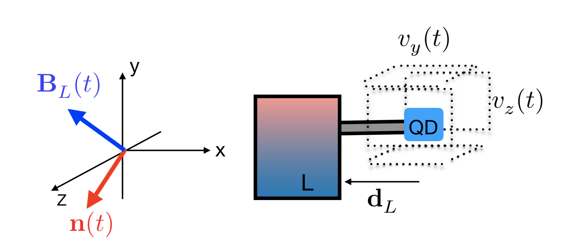
Figure 1: (Color online.) A quantum dot, represented by a single localized energy level, is attached to a non-magnetic metal lead by a weak link along the ${\bf x}$-axis. The four plates represent the application of microwave-induced ac gate voltages, $v_{y}(t)$ and $v_{z}(t)$, which create time-dependent electric fields along the $\hat{\bf y}$ and $\hat{\bf z}$ directions, respectively. The resulting total electric field along the vector $\hat{\bf n}(t)$ can be made to rotate in the $y$-$z$ plane by introducing a phase shift between the oscillating gate voltages. The electric field induces a Rashba interaction in the weak link, that is represented by the effective magnetic field ${\bf B}_{L}(t)$, which is perpendicular to both $\hat{\bf x}$ and $\hat{\bf n}(t)$.

In a weak link with broken inversion symmetry Rashba , the electric field creates a time-dependent Rashba interaction Duckheim , which manifests itself in the form of a phase factor superimposed on the tunneling amplitude. This phase factor, arising from the Aharonov-Casher effect AC , reads

$$V_{L}(t) =\exp[ik_{\rm so}{\bf d}_{L}\times\hat{\bf n}(t)\cdot{\mbox{\boldmath{$\sigma$}}}]\ ,$$ (2)

where ${\bf d}_{L}=-d_{L}\hat{\bf x}$ is the radius-vector from the dot to the lead, see Fig. 1. In Eq. (2), ${\mbox{\boldmath{$\sigma$}}}=[\sigma_{x},\sigma_{y},\sigma_{z}]$ is the vector of the Pauli matrices, and $k_{\rm so}$ represents the strength of the Rashba spin-orbit interaction (in inverse-length units), which is proportional to the ac electric field associated with the microwave radiation. The tunneling Hamiltonian that describes transitions between electronic states in the lead (given by the operator $c^{\dagger}_{{\bf k}\sigma}$ that creates an electron of energy $\epsilon_{k}$, wave vector ${\bf k}$, and spin index $\sigma$) and those on the dot (given by the operator $d^{\dagger}_{\sigma^{\prime}}$ that creates an electron of energy $\epsilon$ with spin index $\sigma^{\prime}$) is

$${\cal H}^{L}_{\rm tun}(t) =J_{L}\sum_{\sigma,\sigma^{\prime}}[V^{\ast}_{L}(t)]_{\sigma\sigma^{\prime}}\sum_{\bf k}d^{\dagger}_{\sigma^{\prime}}c_{{\bf k}\sigma}+{\rm H.c.}$$

$$\sim J_{L}\sum_{\sigma,\sigma^{\prime}}\Big{(}[1-|{\bf B}_{L}(t)|^{2}/2]\delta_{\sigma,\sigma^{\prime}}$$

$$-i[{\mbox{\boldmath{$\sigma$}}}\cdot{\bf B}_{L}(t)]_{\sigma^{\prime}\sigma}\Big{)}\sum_{\bf k}d^{\dagger}_{\sigma^{\prime}}c_{{\bf k}\sigma}+{\rm H.c.}\ ,$$ (3)

up to second order in the spin-orbit coupling $\alpha_{L}=k_{\rm so}d_{L}$ ($J_{L}$ is the tunneling energy scale). The spin-orbit interaction appears as a dimensionless effective magnetic field oscillating with frequency $\Omega$,

$${\bf B}_{L}(t) =e^{i\Omega t}{\bf B}^{-}_{L}+e^{-i\Omega t}{\bf B}^{+}_{L}\ ,$$

$${\bf B}^{\pm}_{L} =(\alpha_{L}/2)[\hat{\bf y}\pm i\gamma\hat{\bf z}]\ ,$$ (4)

that is perpendicular to the direction of the weak link, see Fig. 1.

To this order in $\alpha_{L}$, one identifies two processes in Eq. (3). The first conserves the electronic spin during tunneling, while the second, the effective Zeeman term, involves spin flips accompanied by the absorption or emission of an energy quantum $\Omega$ from the electric field com0 , as manifested in Eqs. (4), using $\hbar=1$. At very low temperatures the absorption transitions dominate (for both the $d^{\dagger}_{\sigma^{\prime}}c_{{\bf k}\sigma}$ term and its hermitian conjugate) in which case Eq. (3) simplifies. In particular,

$${\mbox{\boldmath{$\sigma$}}}\cdot{\bf B}_{L}(t)\approx e^{-i\Omega t}{\mbox{\boldmath{$\sigma$}}}\cdot{\bf B}^{+}_{L}=e^{-i\Omega t}(\alpha_{L}/2)(\sigma_{y}+i\gamma\sigma_{z})\ .$$

Note that

$$\sigma_{y}+i\gamma\sigma_{z}=\sigma^{+}(1+\gamma)/2+\sigma^{-}(1-\gamma)/2\ ,$$

where $\sigma^{\pm}=\sigma_{y}\pm i\sigma_{z}$ are operators that increase ($+$) and lower ($-$) the spin projection in the $\hat{\bf x}$-direction. We may now infer that in a circularly polarized electric field, rotating in the clockwise direction ($\gamma=+1$), absorption transitions lead to an accumulation on the dot of spins whose projections on the $\hat{\bf x}$-axis are positive (spin up), while if the electric field rotates in the anti-clockwise direction ($\gamma=-1$) absorption transitions lead to an accumulation of spins whose projections on the $\hat{\bf x}$-axis are negative (spin down). In a linearly polarized field ($\gamma=0$) there is no preference for either spin projection and no net spin is accumulated. Obviously these qualitative arguments will have to be verified by a detailed calculation, which is carried out in the following.

Quite generally, the magnetization on the dot, given by the (dimensionless) vector ${\bf M}_{d}(t)$ (in units of $-g\mu_{\rm B}/2$, where $g$ is the g-factor of the electron and $\mu_{\rm B}$ is the Bohr magneton), is a priori time-dependent,

$${\bf M}_{d}(t)=\sum_{\sigma,\sigma^{\prime}}\langle d^{\dagger}_{\sigma}(t)[{\mbox{\boldmath{$\sigma$}}}]_{\sigma\sigma^{\prime}}d_{\sigma^{\prime}}(t)\rangle\ ,$$ (5)

and the angular brackets denote quantum averaging with respect to the Hamiltonian of the junction,

$${\cal H}(t)={\cal H}_{0}+{\cal H}^{L}_{\rm tun}(t)\ .$$ (6)

The time-independent Hamiltonian ${\cal H}_{0}$ pertains to the decoupled system,

$${\cal H}_{0}=\sum_{\sigma}\epsilon d^{\dagger}_{\sigma}d_{\sigma}+\sum_{{\bf k},\sigma}\epsilon_{k}c^{\dagger}_{{\bf k}\sigma}c_{{\bf k}\sigma}\ ,$$ (7)

with the first term describing the decoupled dot and the second the decoupled electronic reservoir, assumed to consist of non-polarized free electrons; ${\cal H}^{L}_{\rm tun}(t)$ is given in Eq. (3). The quantum average in Eq. (5) is related to the lesser Keldysh Green’s function on the dot at equal times, defined as

$$[G^{<}_{dd,L}(t,t)]_{\sigma^{\prime}\sigma}\equiv i\langle d^{\dagger}_{\sigma}(t)d_{\sigma^{\prime}}(t)\rangle$$ (8)

This Green’s function is derived com1 in Appendix A, exploiting the Keldysh technique. Inserting Eq. (41) into the definition (5), one finds

$${\bf M}_{d}(t)=2\Gamma_{L}\int\frac{d\omega}{2\pi}f_{L}(\omega){\rm Tr}\{W_{L}(t,\omega){\mbox{\boldmath{$\sigma$}}}\}\ ,$$ (9)

where the trace is carried out in spin space. Here, $\Gamma_{L}$ is the width of the Breit-Wigner resonance formed on the dot due to the coupling with the lead com1 , and $f_{L}(\omega)$ is the Fermi distribution in the lead.

The matrix $W_{L}(t,\omega)$ represents the correlation of the Aharonov-Casher phase factors at different times,

$$W_{L}(t,\omega) =\Big{|}\int^{t}dt_{1}e^{i(\omega-\epsilon+i\Gamma_{L})(t-t_{1})}V^{\dagger}_{L}(t_{1})\Big{|}^{2}\ ,$$ (10)

and is calculated in Appendix A. The dc spin accumulation on the dot results from the corresponding dc part of $W_{L}$ which involves the effective Zeeman interaction, i.e., from the last term on the right hand-side of Eq. (46),

$${\bf M}^{\rm dc}_{d}=2\hat{\bf x}\gamma\alpha^{2}_{L}F_{L}(\Omega)\ ,$$ (11)

where $F_{L}(\Omega)$ is an odd function of $\Omega$,

$$F_{L}(\Omega)=\Gamma_{L}\int\frac{d\omega}{2\pi}f_{L}(\omega)[|D(\omega+\Omega)|^{2}-|D(\omega-\Omega)|^{2}]\ ,$$ (12)

with com3 $|D(\omega)|^{2}=|\omega-\epsilon+i\Gamma_{L}|^{-2}$. This function is depicted in Fig. 2; as seen, the integrand (for $\epsilon>0$) is dominated by the resonance of $D(\omega+\Omega)$ since the Fermi function (at low temperatures) is non-zero only for the negative $\omega^{\prime}$s. In Eq. (11) we have used Eqs. (4) to obtain $2i{\bf B}^{-}_{L}\times{\bf B}^{+}_{L}=-\hat{\bf x}\alpha^{2}_{L}\gamma$. The magnetization accumulated on the dot is indeed along $\hat{\bf x}$, as implied by the heuristic argument above. The probability to magnetize the dot is determined by the polarization of the time-dependent electric field. For a linearly polarized electric field ($\gamma=0$) the effective magnetic field for the absorption process is parallel to that of the emission, ${\bf B}^{-}_{L}\parallel{\bf B}^{+}_{L}$, leading to a vanishing magnetic order. In contrast, for circular or elliptic polarization ($\gamma\neq 0$) there appears a dc magnetization on the dot, which is linear in $\gamma$.

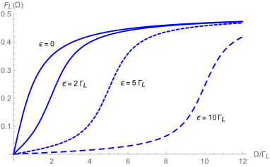
Figure 2: (Color online.) The dimensionless function $F_{L}(\Omega)$ [Eq. (12)] for several values of $\epsilon$ measured with respect to the chemical potential on the lead, for $\Gamma_{L}\beta_{L}=10$, where $\beta_{L}$ is the inverse temperature of the metal lead.

Evidently [see Eq. (9)], the magnetic order built on the dot has also an ac component which oscillates with the frequencies $\Omega$ and $2\Omega$, see Eq. (47). This component gives the temporal variation of the spin polarization on the dot. In the following we add to this component the rate by which the magnetic order is established on the lead, thus examining the total time dependence of the spin population in the entire system.

The magnetization rate in the metal lead, $\dot{\bf M}_{L}(t)$, is defined as

$$\dot{\bf M}_{L}(t)=\frac{d}{dt}\sum_{\bf k}\sum_{\sigma,\sigma^{\prime}}\langle c^{\dagger}_{{\bf k}\sigma}(t)c_{{\bf k}\sigma^{\prime}}(t)\rangle{\mbox{\boldmath{$\sigma$}}}_{\sigma\sigma^{\prime}}\ ,$$ (13)

where the time derivative and the quantum average are with respect to the Hamiltonian (6). This rate can be expressed in terms of lesser Green’s functions, $G^{<}_{Ld}$ and $G^{<}_{dL}$, defined in Eqs. (35),

$$\frac{d}{dt}\sum_{\bf k}\langle c^{\dagger}_{{\bf k}\sigma}(t)c_{{\bf k}\sigma^{\prime}}(t)\rangle =J_{L}[G^{<}_{Ld}(t,t)V^{\dagger}_{L}(t)$$

$$-V_{L}(t)G^{<}_{dL}(t,t)]_{\sigma^{\prime}\sigma}\ .$$ (14)

By solving the corresponding Dyson equations [Eqs. (37)], one obtains this magnetization rate,

$$\dot{\bf M}_{L}(t)={\rm Tr}\{X_{L}(t)V^{\dagger}_{L}(t){\mbox{\boldmath{$\sigma$}}}V_{L}(t)\}\ .$$ (15)

Here we have introduced the matrix

$$X_{L}(t) =i\frac{dG^{<}_{dd,L}(t,t)}{dt}$$

$$=-2\Gamma_{L}\int\frac{d\omega}{2\pi}f_{L}(\omega)\frac{\partial W_{L}(t,\omega)}{\partial t}\ .$$ (16)

[The derivation is contained in Eqs. (52)-(54).] Comparing Eqs. (9) and (15), we find that while the (oscillating) rate of change of the magnetic moment on the dot is

$$\dot{\bf M}_{d}(t)=-{\rm Tr}\{X_{L}(t){\mbox{\boldmath{$\sigma$}}}\}\ ,$$ (17)

that in the lead, Eq. (15), in addition to a sign difference, requires a rotation of $\sigma$ by the Aharonov-Casher phase factors,

$${\mbox{\boldmath{$\sigma$}}}\rightarrow V^{\dagger}_{L}(t){\mbox{\boldmath{$\sigma$}}}V_{L}(t)\ .$$ (18)

The total rate of the spin population in the junction is

$$\dot{\bf M}_{L}(t)+\dot{\bf M}_{d}(t)={\rm Tr}\{X_{L}(t)\big{[}V^{\dagger}_{L}(t){\mbox{\boldmath{$\sigma$}}}V_{L}(t)-{\mbox{\boldmath{$\sigma$}}}\big{]}\}\ ,$$ (19)

and it vanishes only if there is no rotation, i.e., $V_{L}(t)={\bf 1}$. Put differently, the total rate of the spin population along an arbitrary direction $\hat{{\mbox{\boldmath{$\ell$}}}}$, is

$$\hat{{\mbox{\boldmath{$\ell$}}}}\cdot[\dot{\bf M}_{L}(t)+\dot{\bf M}_{d}(t)]=2\Gamma_{L}\int\frac{d\omega}{2\pi}f_{L}(\omega)$$

$$\times{\rm Tr}\Big{\{}\frac{\partial W_{L}(t,\omega)}{\partial t}{\mbox{\boldmath{$\sigma$}}}\cdot[\hat{{\mbox{\boldmath{$\ell$}}}}-\hat{{\mbox{\boldmath{$\ell$}}}}^{\prime}_{L}(t)]\Big{\}}\ ,$$ (20)

where $\hat{{\mbox{\boldmath{$\ell$}}}}^{\prime}_{L}(t)$ is the direction obtained upon rotating $\hat{{\mbox{\boldmath{$\ell$}}}}$ by the Aharonov-Casher phase factors,

$${\mbox{\boldmath{$\sigma$}}}\cdot\hat{{\mbox{\boldmath{$\ell$}}}}^{\prime}_{L}(t)=V^{\dagger}_{L}(t){\mbox{\boldmath{$\sigma$}}}\cdot\hat{{\mbox{\boldmath{$\ell$}}}}V_{L}(t)\ .$$ (21)

The deviation of $\hat{{\mbox{\boldmath{$\ell$}}}}^{\prime}_{L}(t)$ away from $\hat{{\mbox{\boldmath{$\ell$}}}}$ determines the amount by which the magnetization in the entire system is not conserved for a fixed direction, $\hat{{\mbox{\boldmath{$\ell$}}}}$.

Interestingly, the non-conservation has a dc component. Up to second order in the spin-orbit coupling, it suffices to consider the rotation to linear order in the spin-orbit coupling com2

$$\hat{{\mbox{\boldmath{$\ell$}}}^{\prime}}_{L}(t)\sim\hat{{\mbox{\boldmath{$\ell$}}}}+2[{\bf B}^{+}_{L}e^{-i\Omega t}+{\bf B}^{-}_{L}e^{i\Omega t}]\times\hat{{\mbox{\boldmath{$\ell$}}}}\ .$$ (22)

Introducing this expression into Eq. (15) [and making use of Eqs. (21) and (47)], one finds that the total rate in the junction includes two contributions: an oscillating part, which exists in both the lead and in the dot, and a dc part, which exists only in the lead (since the non-oscillating dot magnetization is constant in time), along the $\hat{\bf x}$-axis,

$$\dot{\bf M}_{L}(t)\Big{|}^{\rm dc}=2\hat{\bf x}\gamma\alpha^{2}_{L}\Gamma_{L}\widetilde{F}_{L}(\Omega)\ ,$$ (23)

where

$$\widetilde{F}_{L}(\Omega) =4\Gamma_{L}\Omega^{2}\int\frac{d\omega}{2\pi}f_{L}(\omega)|D(\omega)|^{2}$$

$$\times[|D(\omega+\Omega)|^{2}-|D(\omega-\Omega)|^{2}]\ .$$ (24)

This function is plotted in Fig. 3. As seen, this dc component of the rate is along the $\hat{\bf x}$-axis, just like the dc magnetization on the dot, Eq. (11), both quantities being odd in the microwave frequency, $\Omega$.

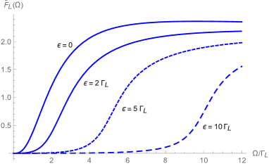
Figure 3: (Color online.) The dimensionless function $\widetilde{F}_{L}(\Omega)$ [Eq. (24)] for several values of $\epsilon$ measured with respect to the chemical potential on the lead, for $\Gamma_{L}\beta_{L}=10$, where $\beta_{L}$ is the inverse temperature of the metal lead.

The total magnetization in the system along a fixed (in time) direction $\hat{{\mbox{\boldmath{$\ell$}}}}$ is not conserved. However, one may examine possible cancellations of the magnetization rates. Adding the magnetization rate in the dot along $\hat{{\mbox{\boldmath{$\ell$}}}}$, to that in the lead along a time-dependent vector given by $\hat{{\mbox{\boldmath{$\ell$}}}}^{\prime\prime}_{L}(t)$,

$${\mbox{\boldmath{$\sigma$}}}\cdot\hat{{\mbox{\boldmath{$\ell$}}}}^{\prime\prime}_{L}(t)=V_{L}(t){\mbox{\boldmath{$\sigma$}}}\cdot\hat{{\mbox{\boldmath{$\ell$}}}}V^{\dagger}_{L}(t)\ ,$$ (25)

results in

$${\rm Tr}\{X_{L}(t)V^{\dagger}_{L}(t){\mbox{\boldmath{$\sigma$}}}\cdot\hat{{\mbox{\boldmath{$\ell$}}}}^{\prime\prime}_{L}(t)V_{L}(t)\}+\dot{\bf M}_{d}(t)\cdot\hat{{\mbox{\boldmath{$\ell$}}}}=0\ ,$$ (26)

which implies that the sum of the spin currents along these specific directions vanishes. The sum of the dot magnetization along $\hat{{\mbox{\boldmath{$\ell$}}}}$ and of the lead magnetization along $\hat{{\mbox{\boldmath{$\ell$}}}}^{\prime\prime}_{L}(t)$ is conserved. This is physically understood: an electron magnetization along $\hat{{\mbox{\boldmath{$\ell$}}}}$ in the dot rotates by the Aharonov-Casher factor to be along $\hat{{\mbox{\boldmath{$\ell$}}}}^{\prime\prime}_{L}(t)$ in the lead.

III A dot coupled to two metal reservoirs

The main reason for extending our scheme to a dot coupled to more than a single lead [see Fig. 4], is to explore the possibility that the induced spin-orbit interaction in, say, the left weak link, will generate a magnetic moment in the right lead. In other words, we wish to find out how the existence of one lead affects the accumulated spin magnetization in the other.

Consider the magnetization rate in the left lead $\dot{\bf M}_{L}(t)$, as defined in Eqs. (13) and (14), when applied to the two-terminal junction depicted in Fig. 4. It is again convenient to express this quantity in terms of the (matrix) function $X_{L}(t)$, cf. Eq. (15). However, in contrast to the configuration dealt with in Sec. II, in the case where the dot is coupled to two leads, $X_{L}(t)$ takes the form

$$X_{L}(t)=2\int\frac{d\omega}{2\pi}\Big{(}-\Gamma_{L}f_{L}(\omega)\frac{\partial W_{L}(t,\omega)}{\partial t}$$

$$+2\Gamma_{L}\Gamma_{R}[f_{R}(\omega)W_{R}(t,\omega)-f_{L}(\omega)W_{L}(t,\omega)]\Big{)}\ .$$ (27)

[This expression results upon inserting Eq. (41) for $G_{dd,L}$–and the corresponding one for $G_{dd,R}$– into Eq. (54).] The analogous function $X_{R}(t)$ is obtained from Eq. (27) by replacing $L$ with $R$.

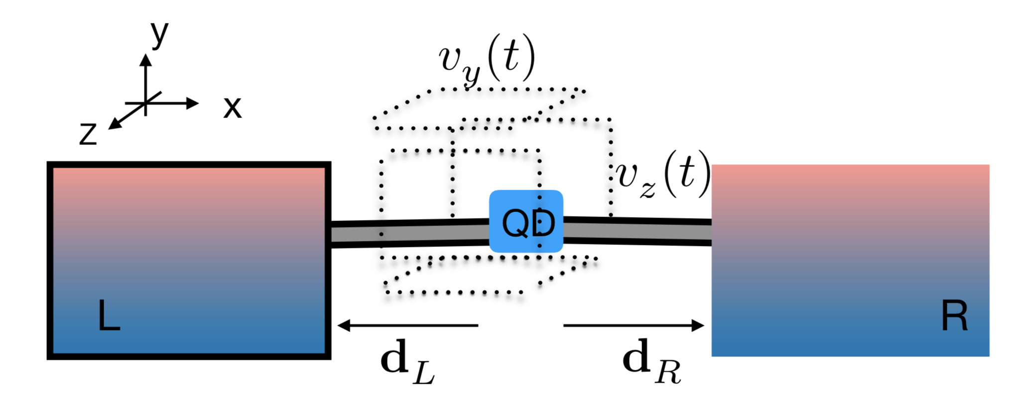
Figure 4: (Color online.) Illustration of a junction comprising a quantum dot, attached by two weak links lying along the $\hat{\bf x}$-axis to two reservoirs, denoted $L$ and $R$. As in Fig. 1, the four plates mark the application of microwave-induced ac gate voltages, $v_{y}(t)$ and $v_{z}(t)$. These give rise to time-dependent spin-orbit interactions in the weak links.

The detailed calculation of the rate $\dot{\bf M}_{L}(t)$ is carried out in Appendix A, see Eq. (55) there. The dc component is presented here,

$$\dot{\bf M}^{\rm dc}_{L}=\hat{\bf x}\Big{(}\gamma\alpha^{2}_{L}[2\Gamma\widetilde{F}_{L}(\Omega)-4\Gamma_{R}F_{L}(\Omega)]$$

$$+\gamma\alpha^{2}_{R}4\Gamma_{L}F_{R}(\Omega)-\gamma\alpha_{L}F_{LR}(\Omega)\Big{)}\ ,$$ (28)

where $F_{L}(\Omega)$ is defined in Eq. (12), $F_{R}(\Omega)$ is derived from the same equation by replacing $L$ with $R$, $\widetilde{F}_{L}(\Omega)$ is defined in Eq. (24), and

$$F_{LR}(\Omega)= 8\Gamma_{L}\Gamma_{R}\int\frac{d\omega}{2\pi}[\alpha_{R}f_{R}(\omega)$$

$$+\alpha_{L}f_{L}(\omega)]2{\rm Re}[D_{3}(\omega)]\ ,$$ (29)

with

$$2{\rm Re}[D_{3}(\omega)] =4|D(\omega-\Omega)D(\omega+\Omega)|^{2}$$

$$\times\Omega(\omega-\epsilon)[1-\Omega^{2}|D(\omega)|^{2}]\ .$$ (30)

Adding the rate of change of the magnetization in the left lead [using Eqs. (15) and the analogous one for the right lead] to the analogous one for the rate of change of the magnetization in the right lead, $\dot{\bf M}_{R}$, yields

$$[\dot{\bf M}_{L}(t)+\dot{\bf M}_{R}(t)]\cdot\hat{{\mbox{\boldmath{$\ell$}}}} ={\rm Tr}\{X_{L}(t)\hat{{\mbox{\boldmath{$\ell$}}}}^{\prime}_{L}(t)\cdot{\mbox{\boldmath{$\sigma$}}}\}$$

$$+X_{R}(t)\hat{{\mbox{\boldmath{$\ell$}}}}^{\prime}_{R}(t)\cdot{\mbox{\boldmath{$\sigma$}}}\}\ ,$$ (31)

where $\hat{{\mbox{\boldmath{$\ell$}}}}$ is again an arbitrary direction, and $\hat{{\mbox{\boldmath{$\ell$}}}}^{\prime}_{L}(t)$, defined in Eq. (21), is the direction reached upon rotating $\hat{{\mbox{\boldmath{$\ell$}}}}$ by the (time-dependent) Aharonov-Casher factors of the left link. Similarly, $\hat{{\mbox{\boldmath{$\ell$}}}}^{\prime}_{R}(t)$ is the direction reached by the rotation with the Aharonov-Casher factors of the right link. The rate of change of the magnetization in the dot, $\dot{\bf M}_{d}(t)$, comprises contributions from the coupling with the left reservoir and the right one (see Appendix A). The first is given in Eq. (9), and the second is obtained from it by replacing $L$ with $R$. Thus, its rate of change is

$$\dot{\bf M}_{d}(t)\cdot\hat{{\mbox{\boldmath{$\ell$}}}}=2\int \frac{d\omega}{2\pi}{\rm Tr}\Big{\{}\Big{(}\Gamma_{L}f_{L}(\omega)\frac{dW_{L}(t,\omega)}{dt}$$

$$+\Gamma_{R}f_{R}(\omega)\frac{dW_{R}(t,\omega)}{dt}\Big{)}{\mbox{\boldmath{$\sigma$}}}\cdot\hat{{\mbox{\boldmath{$\ell$}}}}\Big{\}}\ .$$ (32)

Adding together Eqs. (31) and (32) [using Eq. (27) and the analogous one for $X_{R}(t)$] gives the total rate of change of the magnetization in the two-terminal junction along an arbitrary direction $\hat{{\mbox{\boldmath{$\ell$}}}}$,

$$[\dot{\bf M}_{d}(t)+\dot{\bf M}_{L}(t)+\dot{\bf M}_{R}(t)]\cdot\hat{{\mbox{\boldmath{$\ell$}}}} =2{\rm Tr}\Big{\{}\int\frac{d\omega}{2\pi}\Big{(}\Gamma_{L}f_{L}(\omega)\frac{dW_{L}(t,\omega)}{dt}{\mbox{\boldmath{$\sigma$}}}\cdot[\hat{{\mbox{\boldmath{$\ell$}}}}-\hat{{\mbox{\boldmath{$\ell$}}}}^{\prime}_{L}(t)]+\Gamma_{R}f_{R}(\omega)\frac{dW_{R}(t,\omega)}{dt}{\mbox{\boldmath{$\sigma$}}}\cdot[\hat{{\mbox{\boldmath{$\ell$}}}}-\hat{{\mbox{\boldmath{$\ell$}}}}^{\prime}_{R}(t)]\Big{)}\Big{\}}$$

$$+4\Gamma_{L}\Gamma_{R}{\rm Tr}\Big{\{}\int\frac{d\omega}{2\pi}[f_{L}(\omega)W_{L}(t,\omega)-f_{R}(\omega)W_{R}(t,\omega)][\hat{{\mbox{\boldmath{$\ell$}}}}^{\prime}_{R}(t)-\hat{{\mbox{\boldmath{$\ell$}}}}^{\prime}_{L}(t)]\cdot{\mbox{\boldmath{$\sigma$}}}\Big{\}}\ .$$ (33)

As found in Sec. II, the total magnetization would have been conserved had the rotations of the spin on their way between the dot and the leads been ignored. The amount by which the total magnetization is not conserved when measured along a fixed (time-independent) direction $\hat{{\mbox{\boldmath{$\ell$}}}}$ is determined by the rotations of this direction from the dot to the left lead and to the right one. Thus, the time-dependent spin-orbit coupling generate a time-independent magnetization, and the amount by which it is not conserved has also a dc part.

IV Discussion

We propose that inelastic tunneling of electrons through a weak link, accompanied by spin flips generated by a spin-orbit coupling caused by a rotating electric field, is capable of producing a net spin population in a nonmagnetic device; the field can be induced by microwave radiation as indicated in Fig. 1. The origin of this effect is the correlation between emission and absorption of photons by tunneling electrons and specific spin flips (from spin down to spin up or from spin up to spin down). Our conjecture was verified in Sec. II for a single-level quantum dot coupled to a nonmagnetic reservoir of electrons, in the particular case when the dot energy level, $\epsilon$, is situated above the Fermi energy, $\epsilon_{F}$, of the reservoir and hence is unoccupied at zero temperature. However, one can easily convince oneself that the effect is the same if the dot level is situated below the the Fermi energy, $\epsilon<\epsilon_{F}$, so that the dot level is doubly occupied at zero temperature.

We would like to remind the reader that our calculation is carried out in the weak electron tunneling limit. This means that the probability for double occupancy of an initially empty dot (the case discussed above) due to inelastic tunneling is negligibly small. Therefore, the intra-dot Coulomb repulsion energy $U$ in a doubly occupied dot does not enter the calculation. By the same argument, if the dot is initially doubly occupied only one electron can be removed due to inelastic tunneling in the weak tunneling limit. In this case the Coulomb energy $U$ does play a role, since the energy cost of removing one electron from the dot is $\epsilon_{F}-(\epsilon+U)$ (compared to the energy $\epsilon-\epsilon_{F}$ required to add one electron to an empty dot). This allows one to expect that if the dot contains several energy levels that can be involved in photon-assisted spin-flip transitions, the amount of spin accumulation on the dot can be augmented compared to when the dot has only one level. Except for this difference, the role of the interaction energy is trivial.

As discussed in Sec. II, photon absorption processes dominate at low temperatures. For a circularly polarized electric field rotating in, say, the clockwise direction (in the sense defined in Sec. II) the requirement that spin angular momentum is conserved then only allows spins to flip from “down" to “up". For an unoccupied dot, $\epsilon>\epsilon_{F}$, this means that only transitions from an occupied electron state with spin down in the reservoir to the spin-up state in the dot are allowed. If, on the other hand $\epsilon<\epsilon_{F}$, only transitions from an occupied spin-down state in the dot to an unoccupied electron spin-up state in the reservoir are allowed, leaving an uncompensated spin-up electron on the dot. Consequently, inelastic transitions between electron states in the lead and both occupied ($\epsilon<\epsilon_{F}$) and unoccupied ($\epsilon>\epsilon_{F}$) dot states result in the same spin state on the dot. This allows one to expect that if the dot contains several energy levels that can be involved in photon-assisted spin-flip transitions, the amount of spin accumulation on the dot can be augmented compared to when the dot has only one level.

Driving the electron spin dynamics by a rotating electric field as suggested in this paper represents only one of several options for achieving a time-dependent spin-orbit coupling in nanodevices. Another possibility is to use a mechanical drive by temporally modulating the geometry of the device Shekhter . A related recent theoretical idea Murakami proposes to exploit externally excited chiral phonon modes in graphene (which cause the carbon atoms to rotate and hence the spin-orbit interaction to be time dependent) to accumulate spin and generate magnetization.

The Keldysh Green’s function for the dot, defined in Eq. (8), can be viewed as the spin density matrix of a spin q-bit. Its quantum coherent dynamics is fully determined by the time dependence of the spin-orbit interaction, which is induced by the ac gate voltages [see Eq. (53)]. Hence, driving the device by microwaves as envisaged here offers the possibility to create and manipulate a spin q-bit by applying appropriate microwave pulses as is well-known from the field of quantum computing.

The results presented in this paper open the possibility to use microwave radiation to activate a magnetic pattern at the surface of a conductor. An array of quantum dots could be deposited on the surface, each dot individually coupled to the conductor by spin-orbit-active tunnel junctions. The magnetization of each dot could in principle be controlled locally by electrostatic gates or by mechanical deformations of the tunneling weak links. In this way, one might be able to create a multiple q-bit structure in which communication between the dots would be governed by spin currents flowing between the dots and the common reservoir. A study of such possibilities is well beyond the scope of the present paper, but might serve as a motivation for further investigations of the possibility to create static magnetization by irradiation with microwaves.

Appendix A Technical details

1. The Green’s functions in the time domain. For a dot coupled to two leads (Fig. 4), the Hamiltonian (7) is augmented by a term describing the right lead, $\sum_{{\bf p},\sigma}\epsilon_{p}c^{\dagger}_{{\bf p}\sigma}c_{{\bf p}\sigma}$. In addition, the tunneling Hamiltonian in Eq. (6) includes a term yielding the tunneling between the dot and the right lead which takes the same form as in Eq. (3), with ${\bf k}$ replaced by ${\bf p}$ and $L$ by $R$. [Note that ${\bf d}_{R}=\hat{\bf x}d_{R}$ and consequently ${\bf B}_{R}(t)/\alpha_{R}=-{\bf B}_{L}(t)/\alpha_{L}$.]

The Dyson equation for the Green’s function on the dot, $G_{dd}(t,t^{\prime})$ (in matrix notations in spin space), reads

$$G_{dd}(t,t^{\prime})=g_{d}(t,t^{\prime}) +\int dt_{1}g_{d}(t,t_{1})[J_{L}V^{\dagger}_{L}(t_{1})G_{Ld}(t_{1},t^{\prime})$$

$$+J_{R}V^{\dagger}_{R}(t_{1})G_{Rd}(t_{1},t^{\prime})]\ .$$ (34)

The first term in the square brackets results from the tunnel coupling with the left lead [see Eq. (3)], and the second comes from the tunnel coupling with the right lead. The two other Green’s functions introduced in Eq. (34) are

$$G_{dL}(t,t^{\prime}) =\sum_{\bf k}G_{d{\bf k}}(t,t^{\prime})\ ,$$

$$G_{Ld}(t,t^{\prime}) =\sum_{\bf k}G_{{\bf k}d}(t,t^{\prime})\ ,$$ (35)

(with analogous definitions for $G_{dR}$ and $G_{Rd}$). The Dyson’s equation (34), as all other encountered below, refer to all three Keldysh Green’s functions, the lesser (superscript $<$), the retarded (superscript $r$), and the advanced (superscript $a$) Langreth ; Jauho . In Eq. (34), $g_{d}(t,t^{\prime})$ is the Green’s function of the isolated dot; its retarded and advanced forms are

$$g^{r(a)}_{d}(t,t^{\prime}) =\mp i\Theta(\pm t\mp t^{\prime})\exp[-i\epsilon(t-t^{\prime})]\ ,$$ (36)

while the lesser function is zero since the isolated dot is assumed to be empty.

The Dyson’s equations for the Green’s functions (35) read (in matrix notations in spin space)

$$G_{Ld}(t,t^{\prime}) =J_{L}\int dt_{1}g_{L}(t,t_{1})V_{L}(t_{1})G_{dd}(t_{1},t^{\prime})\ ,\ \$$

$$G_{dL}(t,t^{\prime}) =J_{L}\int dt_{1}G_{dd}(t,t_{1})V^{\dagger}_{L}(t_{1})g_{L}(t_{1},t^{\prime})\ ,$$ (37)

where $g_{L}(t,t^{\prime})$ is Green’s function of the decoupled left lead. Within the wide-band approximation Meir , the retarded, advanced, and lesser functions of the latter are

$$g^{r(a)}_{L}(t,t^{\prime}) =\mp i\pi{\cal N}_{L}\delta(t-t^{\prime})\ ,$$ (38)

and

$$g^{<}_{L}(t,t^{\prime}) =i\sum_{k}e^{-i\epsilon_{k}(t-t^{\prime})}f_{L}(\epsilon_{k})$$

$$=2\pi i{\cal N}_{L}\int\frac{d\omega}{2\pi}e^{-i\omega(t-t^{\prime})}f_{L}(\omega)\ .$$ (39)

The density of states of the left lead at the Fermi energy is denoted ${\cal N}_{L}$, and $f_{L}(\epsilon_{k})$ is the Fermi function there.

The physical quantities studied in the main text involve the lesser Green’s functions at equal times. Straightforward manipulations of Eqs. (34) and (37) yield that $G^{<}_{dd}(t,t)$ comprises contributions from the coupling of the dot to the left and right leads,

$$G^{<}_{dd}(t,t)=G^{<}_{dd,L}(t,t)+G^{<}_{dd,R}(t,t)\ ,$$ (40)

where

$$G^{<}_{dd,L}(t,t) =2i\Gamma_{L}\int\frac{d\omega}{2\pi}f_{L}(\omega)W_{L}(t,\omega)\ .$$ (41)

(For more details, see Refs. Odashima, and PreSM, .) Here, $\Gamma_{L}=2\pi J^{2}_{L}{\cal N}_{L}$ is the partial width of the resonance on the dot, created by the tunnel coupling with the left lead. An analogous expression pertains for $G^{<}_{dd,R}(t,t)$. The total resonance width on the dot is $\Gamma=\Gamma_{L}+\Gamma_{R}$.

The key player in our scheme is the 2$\times$2 matrix in spin space, $W_{L}(t,\omega)$, defined in Eq. (10). Exploiting the expression for $V^{\dagger}_{L}(t)$ valid for a weak spin-orbit coupling [see Eq. (3)], we find

$$\int^{t}dt_{1}e^{i(\omega-\epsilon+i\Gamma)(t-t_{1})}[1-|{\bf B}_{L}(t_{1})|^{2}/2-i{\mbox{\boldmath{$\sigma$}}}\cdot{\bf B}_{L}(t_{1})]$$

$$=D(\omega)[1-(1+\gamma^{2})\alpha^{2}_{L}/4]-[(1-\gamma^{2})\alpha^{2}_{L}/4]F_{2}(t,\omega)$$

$$-i{\mbox{\boldmath{$\sigma$}}}\cdot[{\bf B}^{-}_{L}e^{i\Omega t}D(\omega-\Omega)+{\bf B}^{+}_{L}e^{-i\Omega t}D(\omega+\Omega)]\ ,$$ (42)

where $D(\omega)$ is com3

$$D(\omega) =i/[\omega-\epsilon+i\Gamma]\ ,$$ (43)

and

$$F_{2}(t,\omega) =\frac{1}{2}[e^{i2\Omega t}D(\omega-2\Omega)+e^{-i2\Omega t}D(\omega+2\Omega)]\ .$$ (44)

Using the result (42) in Eq. (10), one finds that

$$W_{L}(t,\omega)=W^{\rm dc}_{L}(\omega)+W^{\rm ac}_{L}(t,\omega)\ ,$$ (45)

where $W^{\rm dc}_{L}(\omega)$ does not depend on time,

$$W^{\rm dc}_{L}(\omega)=|\widetilde{D}(\omega)|^{2}+iD_{1}(\omega){\mbox{\boldmath{$\sigma$}}}\cdot{\bf B}^{-}_{L}\times{\bf B}^{+}_{L}\ ,$$ (46)

and $W^{\rm ac}_{L}(t,\omega)$ oscillates with frequencies $\Omega$ and $2\Omega$,

$$W^{\rm ac}_{L}(t,\omega)={\bf B}^{-}_{L}\cdot{\bf B}^{-}_{L}e^{2i\Omega t}D_{2}(\omega)+{\rm c.c.}$$

$$+i{\mbox{\boldmath{$\sigma$}}}\cdot[{\bf B}^{+}_{L}e^{-i\Omega t}D_{3}(\omega)-{\rm c.c.}]\ .$$ (47)

The function $|\widetilde{D}(\omega)|^{2}$ in Eq. (46)

$$|\widetilde{D}(\omega)|^{2} =|D(\omega)|^{2}-(1+\gamma^{2})(\alpha^{2}_{L}/2)\Big{(}|D(\omega)|^{2}$$

$$-[|D(\omega-\Omega)|^{2}+|D(\omega+\Omega)|^{2}]/2\Big{)}\ ,$$ (48)

is the correction (due to the spin-orbit coupling) of the Breit-Wigner resonance on the dot. The other functions in Eqs. (46) and (47) are

$$D_{1}(\omega) =|D(\omega-\Omega)|^{2}-|D(\omega+\Omega)|^{2}\ ,$$

$$D_{2}(\omega) =[(\omega-\epsilon)^{2}-(\Omega-i\Gamma)^{2}]^{-1}$$

$$-[1+4i\Gamma\Omega|D(\omega)|^{2}][(\omega-\epsilon)^{2}-(2\Omega-i\Gamma)^{2}]^{-1}\ ,$$

$$D_{3}(\omega) =|D(\omega)|^{2}[2\Omega(\omega-\epsilon)][(\omega-\epsilon)^{2}-(\Omega+i\Gamma)^{2}]^{-1}\ ,$$ (49)

and they all vanish when $\Omega=0$.

2. The magnetization rates in the leads. By solving the Dyson’s equations (37), the magnetization rate in the left lead, given in Eqs. (13) and (14), can be expressed in terms of the Green’s functions on the dot PreSM ,

$$\frac{d}{dt}\sum_{\bf k}\langle c^{\dagger}_{{\bf k}\sigma}(t)c_{{\bf k}\sigma^{\prime}}(t)\rangle=-2i\Gamma_{L}\Big{(}[V_{L}(t)G^{<}_{dd}(t,t)V^{\dagger}_{L}(t)]_{\sigma^{\prime}\sigma}$$

$$-\int\frac{d\omega}{2\pi}f_{L}(\omega)$$

$$\times\int dt_{1}[e^{-i\omega(t-t_{1})}V_{L}(t_{1})G^{a}_{dd}(t_{1},t)V^{\dagger}_{L}(t)-{\rm H.c.}]_{\sigma^{\prime}\sigma}\Big{)}\ .$$ (50)

This expression is conveniently written in the form

$$\frac{d}{dt}\sum_{\bf k}\langle c^{\dagger}_{{\bf k}\sigma}(t)c_{{\bf k}\sigma^{\prime}}(t)\rangle=[V_{L}(t)X_{L}(t)V^{\dagger}_{L}(t)]_{\sigma^{\prime}\sigma}\ ,$$ (51)

where

$$X_{L}(t)=-2i\Gamma_{L}G^{<}_{dd}(t,t)+2i\Gamma_{L}\int\frac{d\omega}{2\pi}f_{L}(\omega)$$

$$\times\int dt_{1}[e^{-i\omega(t-t_{1})}V^{\dagger}_{L}(t)V_{L}(t_{1})G^{a}_{dd}(t_{1},t)-{\rm H.c.}]\ .$$ (52)

The advantage of this representation is revealed when Eqs. (41) and (10) are used to find

$$\frac{d}{dt}G^{<}_{dd,L}(t,t)=-2\Gamma G^{<}_{dd,L}(t,t)+2\Gamma_{L}\int\frac{d\omega}{2\pi}f_{L}(\omega)$$

$$\times\int dt_{1}[V^{\dagger}_{L}(t)e^{-i\omega(t-t_{1})}V_{L}(t_{1})G^{a}_{dd}(t_{1},t)-{\rm H.c.}]\ .$$ (53)

It then follows that

$$X_{L}(t) =idG^{<}_{dd,L}(t,t)/dt$$

$$+2i[\Gamma_{R}G^{<}_{dd,L}(t,t)-\Gamma_{L}G^{<}_{dd,R}(t,t)]\ .$$ (54)

For the single-lead junction, considered in Sec. II, $\Gamma_{R}=0$, and therefore only the first term on the right hand-side of Eq. (54) survives. The corresponding expression for the two-terminal junction is obtained upon inserting Eqs. (40) and (41) in Eq. (54); this yields Eq. (27) in the main text.

The explicit expression for the magnetization rate in the left lead is obtained by using Eq. (27) in Eq. (15). Denoting for brevity $\hat{{\mbox{\boldmath{$\ell$}}}^{\prime}}_{L}(t)=V^{\dagger}_{L}(t)\hat{{\mbox{\boldmath{$\ell$}}}}V_{L}(t)$, and using Eqs. (46) and (47), we find

$$\dot{\bf M}_{L}(t)\cdot\hat{{\mbox{\boldmath{$\ell$}}}} =-4i\Gamma_{L}\int\frac{d\omega}{2\pi}f_{L}(\omega)\hat{{\mbox{\boldmath{$\ell$}}}^{\prime}}_{L}(t)\cdot\frac{d}{dt}[{\bf B}^{+}_{L}e^{-i\Omega t}D_{3}(\omega)-{\rm c.c.}]$$

$$+8i\Gamma_{L}\Gamma_{R}\int\frac{d\omega}{2\pi}D_{1}(\omega)[{\bf B}^{-}_{R}\times{\bf B}^{+}_{R}f_{R}(\omega)-{\bf B}^{-}_{L}\times{\bf B}^{+}_{L}f_{L}(\omega)]\cdot\hat{{\mbox{\boldmath{$\ell$}}}^{\prime}}_{L}(t)$$

$$-8i\Gamma_{L}\Gamma_{R}\int\frac{d\omega}{2\pi}\Big{(}f_{R}(\omega)[{\bf B}^{+}_{R}e^{-i\Omega t}D_{3}(\omega)-{\rm c.c.}]-f_{L}(\omega)[{\bf B}^{+}_{L}e^{-i\Omega t}D_{3}(\omega)-{\rm c.c.}]\Big{)}\cdot\hat{{\mbox{\boldmath{$\ell$}}}^{\prime}}_{L}(t)\ ,$$ (55)

where the functions $D_{1}(\omega)$ and $D_{3}(\omega)$ are defined in Eqs. (49). The dc magnetization rate (to second order in the spin-orbit coupling) is

$$\dot{\bf M}^{\rm dc}_{L}\cdot\hat{{\mbox{\boldmath{$\ell$}}}} =-8i\Gamma_{L}\Omega{\bf B}^{+}_{L}\times{\bf B}^{-}_{L}\cdot\hat{{\mbox{\boldmath{$\ell$}}}}\int\frac{d\omega}{2\pi}f_{L}(\omega)2{\rm Im}[D_{3}(\omega)]$$

$$+8i\Gamma_{L}\Gamma_{R}\int\frac{d\omega}{2\pi}D_{1}(\omega)[{\bf B}^{-}_{R}\times{\bf B}^{+}_{R}f_{R}(\omega)-{\bf B}^{-}_{L}\times{\bf B}^{+}_{L}f_{L}(\omega)]\cdot\hat{{\mbox{\boldmath{$\ell$}}}}$$

$$+16i\Gamma_{L}\Gamma_{R}\Big{(}{\bf B}^{+}_{R}\times{\bf B}^{-}_{L}\cdot\hat{{\mbox{\boldmath{$\ell$}}}}\int\frac{d\omega}{2\pi}f_{R}(\omega)D_{3}(\omega)+{\bf B}^{+}_{L}\times{\bf B}^{-}_{R}\cdot\hat{{\mbox{\boldmath{$\ell$}}}}\int\frac{d\omega}{2\pi}f_{R}(\omega)D^{\ast}_{3}(\omega)\Big{)}$$

$$-16i\Gamma_{L}\Gamma_{R}{\bf B}^{+}_{L}\times{\bf B}^{-}_{L}\cdot\hat{{\mbox{\boldmath{$\ell$}}}}\int\frac{d\omega}{2\pi}f_{L}(\omega)2{\rm Re}[D_{3}(\omega)]\ .$$ (56)

As ${\bf B}^{\pm}_{L}/\alpha_{L}=-{\bf B}^{\pm}_{R}/\alpha_{R}$, and by Eqs. (49)

$$2{\rm Re}[D_{3}(\omega)]=4|D(\omega-\Omega)D(\omega+\Omega)|^{2}\Omega(\omega-\epsilon)[1-\Omega^{2}|D(\omega)|^{2}]\ ,$$

$$2{\rm Im}[D_{3}(\omega)]=2\Gamma\Omega|D(\omega)|^{2}[|D(\omega-\Omega)|^{2}-|D(\omega+\Omega)|^{2}]\ ,$$ (57)

the rate $\dot{\bf M}^{\rm dc}_{L}$ takes the form given in Eq. (28).

References

- (1) D. Sander, S. O. Valenzuela, D. Makarov, C. H. Marrows, E. E. Fullerton, P. Fischer, J. McCord, P. Vavassori, S. Mangin, P. Pirro, B. Hillebrands, A. D. Kent, T. Jungwirth, O. Gutfleisch, C. G. Kim, and A. Berger, The 2017 Magnetism Roadmap, J. Phys. D: Appl. Phys. 50, 363001 (2017).
- (2) B. J. Kirby, L. Fallarino, P. Riego, B. B. Maranville, C. W. Miller, and A. Berger, Nanoscale magnetic localization in exchange strength modulated ferromagnets, Phys. Rev. B 98, 064404 (2018).
- (3) See e.g., J. M. Miron, G. Gaudin, S, Auffret, B. Rodmacq, A, Schuhl, S. Pizzini, J. Vogel, and P. Gambardella, Current-driven spin torque induced by the Rashba effect in a ferromagnetic metal layer, Nature Materials 9, 230 (2010).
- (4) S. Pile, M. Buchner, V. Ney, T. Schaffers, K. Lenz, R. Narkowicz, J. Lindner, H. Ohldag, and A. Ney, Direct imaging of the ac component of the pumped spin polarization with element specificity, arXiv:2005.08728v1 (2020).
- (5) Y. Araki , T. Misawa , and K. Nomura, Dynamical spin-to-charge conversion on the edge of quantum spin Hall insulator, Phys. Rev. Research 2, 023195 (2020).
- (6) E. I. Rashba, Properties of semiconductors with an extremum loop .1. Cyclotron and combinational resonance in a magnetic field perpendicular to the plane of the loop, Fiz. Tverd. Tela (Leningrad) 2, 1224 (1960) [Sov. Phys. Solid State 2, 1109 (1960)]; Y. A. Bychkov and E. I. Rashba, Oscillatory effects and the magnetic susceptibility of carriers in inversion layers, J. Phys. C 17, 6039 (1984).
- (7) V. M. Edelstein, Spin polarization of conduction electrons induced by electric current in two-dimensional asymmetric electron systems, Solid State Commun. 73, 233 (1990).
- (8) J. C. Rojas Sánchez, L. Vila, G. Desfonds, S. Gambarelli, J. P. Attanné, J. M. De Teresa, C. Magén, and A. Fert, Spin-to-charge conversion using Rashba coupling at interface between non-magnetic materials, Nature Comm. 4, 2944 (2013).
- (9) L. Salemi, M. Berritta, A. K. Nandy, and P. M. Oppeneer, Orbitally dominated Rashba-Edelstein effect in noncentrosymmetric antiferromagnets, Nature Comm. 10, 1038 (2019).
- (10) J. Puebla, F. Auvray, N. Yamaguchi, M. Xu, S. Zulkarnaen Bisri, Y. Iwasa, F. Ishii, and Y. Otani, Photoinduced Rashba spin-to-charge conversion via interfacial unoccupied state, Phys. Rev. Lett. 122, 256401 (2019).
- (11) D. Hernangómez-Pérez, J. D. Torres, and A. López, Photoinduced electronic and spin properties of quantum Hall systems with Rashba spin-orbit coupling, arXiv:2005.05450v1 (2020).
- (12) Y. Aharonov and A. Casher, Topological quantum Effects for Neutral Particles, Phys. Rev. Lett. 53, 319 (1984).
- (13) R. I. Shekhter, O. Entin-Wohlman, and A. Aharony, Suspended nanowires as mechanically-controlled Rashba spin-splitters, Phys. Rev. Lett. 111, 176602 (2013).
- (14) J. H. Bardarson, A proof of the Kramers degeneracy of transmission eigenvalues from antisymmetry of the scattering matrix, J. Phys. A: Math. Theor. 41, 405203 (2008).
- (15) O. Entin-Wohlman, R. I. Shekhter, M. Jonson, and A. Aharony, Photovoltaic effect generated by spin-orbit interactions, Phys. Rev. B 101, 121303(R) (2020).
- (16) M. Duckheim and D. Loss, Electric Dipole Induced Spin Resonance in Disordered Semiconductors, Nature Phys. 2, 195 (2006).
- (17) Although we treat the electric field classically, a time-dependent quantum-mechanical perturbation theory with the Hamiltonian (3) will generate inelastic transitions to electron states with flipped spins and with energy shifted by only. We can therefore refer to these energy quanta as ‘photons’.
- (18) The calculations in Appendix A are carried out for a dot coupled to two leads, see Fig. 4. However, it is straightforward to infer from the expressions in Appendix A the relevant quantities for the simpler junction depicted in Fig. 1: all that one needs to do is to set , the partial resonance width on the dot resulting from the coupling to the right lead, to zero.
- (19) The resonance width in is when the dot is coupled to a single lead. For the two-terminal junction, the resonance width is , see Appendix A.
- (20) It is sufficient to consider the rotation transformation to first order in the spin-orbit coupling, since the other terms in Eq. (17) that contribute to the trace are at least first order in .
- (21) R. I. Shekhter, O. Entin-Wohlman, M. Jonson, and A. Aharony, Rashba spin-splitting of single electrons and Cooper pairs, Low Temp. Phys. 43, 303 (2017); Photo-spintronics of spin-orbit active electric weak links, ibid. 43, 910 (2017).
- (22) M. Hamada and S. Murakami, Conversion between electron spin and microscopic atomic rotation, Phys. Rev. Research 2, 023275 (2020).
- (23) D. C. Langreth, Linear and nonlinear response theory with applications, in Linear and Nonlinear Electron Transport in Solids, eds. J. T. Devreese and E. van Boren (Plenum, New York, 1976).
- (24) A. P. Jauho, Nonequilibrium Green function modelling of transport in mesoscopic systems, in Progress in Nonequilibrium Green’s Functions II, eds. M. Bonitz and D. Semkat (World Scientific, Singapore, 2003).
- (25) A-P. Jauho, N. S. Wingreen, and Y. Meir, Time-dependent transport in interacting and noninteracting resonant-tunneling systems, Phys. Rev. B 50, 5528 (1994).
- (26) M. M. Odashima and C. H. Lewenkopf, Time-dependent resonant tunneling transport: Keldysh and Kadanoff-Baym nonequilibrium Green’s functions in an analytically soluble problem, Phys. Rev. B 95, 104301 (2017).
- (27) See Supplemental Material at http://link.aps.org/supplemental/10.1103/PhysRevB.101.121303 for details of the Keldysh Green’s functions’ calculation.