Strongly lensed SN Refsdal: refining time delays based on the supernova explosion models

Abstract

We explore the properties of supernova (SN) ‘‘Refsdal’’ - the first discovered gravitationally lensed SN with multiple images. A large magnification provided by the galactic-scale lens, augmented by the cluster lens, gave us a unique opportunity to perform a detailed modelling of a distant SN at $z\simeq 1.5$. We present results of radiation hydrodynamics modelling of SN Refsdal. According to our calculations, the SN Refsdal progenitor is likely to be a more massive and energetic version of SN 1987A, i.e. a blue supergiant star Reconstruction of SN light curves allowed us to obtain time delays and magnifications for the images S2-S4 relative to S1 with higher accuracy than previous of Rodney et al. (2016). We estimate the Hubble constant $H_{0}=68.6^{+13.6}_{-9.7}$ km s^-1 Mpc^-1 via re-scaling the time delays predicted by different lens models to match the values obtained in this work. With more photometric data on the fifth image SX, we will be able to further refine the time delay and magnification estimates for SX and obtain competitive constraints on $H_{0}$.

1 Introduction

Supernova explosions are among the most energetic and fascinating phenomena in the Universe. Investigating these objects is essential not only for understanding the physics of stellar explosions, but also for studying properties of progenitor population, stellar evolution, nucleosynthesis, modeling chemical evolution of galaxies, origin of cosmic rays, to name a few. Throughout modern astrophysics, supernovae (SNe) have been also used to measure cosmological distances. Due to high intrinsic brightness and ‘‘standardizable’’ light curves (LCs), SN Ia are now routinely used to determine cosmological parameters. It was by using SNe Ia that Riess et al. (1998) and Perlmutter et al. (1999) discovered an accelerated expansion of the Universe. Observations of type II SNe can be also used to determine distances to their host galaxies. Despite the fact that SNe II show a large variations in their observational properties (luminosities, durations, etc.), there are a number of methods to utilize observations of SN II for cosmological studies (see, e.g., Nugent & Hamuy, 2017, for a review). For instance, the Expanding Photosphere Method (EPM) was proposed by Kirshner & Kwan (1974) to measure distances to the Type II plateau supernovae whose light curve is nearly flat for $\sim$ 100 days and then suddenly drops off. The EPM has been successfully applied to nearby SN IIP (e.g. Tsvetkov et al., 2019) and more distant objects (up to $z\simeq 0.34$; Gall et al. 2018). Other techniques include the Spectral-fitting Expanding Atmosphere Method (e.g. Baron et al., 2004) for SN IIP and the Dense Shell Method (Potashov et al., 2013; Baklanov et al., 2013) to measure distances to SN IIn supernovae.

One of the current frontiers in SNe research centers is constructing numerical models of SNe explosions, reliability of which can be determined from comparison with observational data. Such SN modelling requires high-quality photometric and spectroscopic data. While for super-luminous SNe such detailed information can be in principle obtained even at high redshifts $z>2$ (Cooke et al., 2012), this is not the case for type IIP SNe, which are typically observed up to $z\sim 0.4$ (Nugent & Hamuy, 2017). So far, hydrodynamical models of type IIP supernovae were constructed only for nearby objects.

Recent discovery of gravitationally lensed supernovae with multiple images – SN Refsdal (Kelly et al., 2015) and SN iPTF16geu (Goobar et al., 2017) – opens up a window to the unexplored high-redshift transient universe. Strongly lensed supernovae represent a class of objects unique both for astrophysics and cosmology. They make possible not only investigation of the properties of supernova progenitors (pre-supernovae) and their environments at high redshifts (a signal from which would not be detected in the absence of a lens), but they can be also used for cosmological studies. In a case of a variable source such as a supernova, light curves for different images are shifted in time relative to each other. By measuring these time delays between images, one can obtain an independent estimate the Hubble constant (first suggested by Refsdal 1964) and the dark energy equation of state (e.g. Linder, 2011). For certain types of SNe II and for SN Ia, the intrinsic luminosities can be inferred independently of lensing. In such cases, the absolute lensing magnification can be constrained independently of a lens model, thus helping to break the degeneracy between the radial mass profile of a lens and the Hubble constant (Oguri & Kawano, 2003). Indeed, numerous studies of lensed quasars have convincingly shown the Hubble constant value is sensitive to details of a lens model (e.g. Kochanek, 2002; Larchenkova et al., 2011; Birrer et al., 2016; Wong et al., 2020, among others) and assuming a power-law density distribution (the simplest lens model) introduces a bias in the determination of $H_{0}$ (e.g. Xu et al., 2016).

This paper is devoted to radiation-hydrodynamics modelling of the first discovered lensed supernova with multiple images – SN Refsdal. Kelly et al. (2016) has already shown that the spectra and light curve of SN Refsdal are similar to those of SN 1987A, a peculiar SN II in the Large Magellanic Cloud, and that the progenitor of SN Refsdal is most likely to be a blue supergiant star. As emphasized in Rodney et al. (2016), none of existing light curve templates is able to capture all the features of SN Refsdal light curve, thus making the task of modelling of SN Refsdal important. Moreover, SN Refsdal was located in the arm of a spiral host galaxy at $z\simeq 1.5$, i.e. much farther away than any modelled Type II SNe so far. The construction of a physical model of the pre-supernova, which satisfies available photometric observations in different filters, should in principle allow one to determine time delays between images more accurately than it is done in Rodney et al. (2016) and to constrain the magnification factors. This information can serve as an independent test of different lens models presented in the literature (see Treu et al., 2016, for a compilation of lens models) and/or used as an additional constraint to improve the lens model. The latter should lead to an improved precision in determining the Hubble constant and other cosmological parameters (e.g., Grillo et al., 2018, 2020). The paper is organized as follows. In Section 2, we list available observational data on SN Refsdal. Section 3 gives a brief description of constructed hydrodynamical SN models, the best-fit model which matches all available observational data is described in Section 3.1 Technical details on the fitting procedure are given in Appendix A. We use the reconstructed SN Refsdal to derive time delay and magnification ratios for all images in Section 4. With these estimates in hand, we obtain the most likely Hubble constant value in Section 5. Finally, all the results of this work are summarized in Section 6.

2 Observations

A strongly lensed supernova was found in the MACS J1149.6+2223 galaxy cluster field on 10 November 2014 (Kelly et al., 2015). The HST images revealed four resolved images of the background SNe ($z=1.49$) arranged in an Einstein cross configuration around a massive elliptical galaxy ($z=0.54$) – MACS J1149.6+2223 cluster member.

To construct a hydrodynamic model SN Refsdal, we use photometric data from Rodney et al. (2016) (their Table 4) obtained with HST using the Wide-Field Camera 3 (WFC3) with the infrared (IR) and UV-optical (UVIS) detectors, and the Advanced Camera for Surveys (ACS).

The dynamical properties of the envelope and characteristic expansion velocities can be obtained by investigating line profiles in the spectra of the supernova. Thanks to gravitational amplification of the SN Refsdal light, there are HST, Keck, and VLT X-shooter spectra (Kelly et al., 2016) available. Despite being noisy, these spectral observations give us constraints on how the velocity of the envelope was changing during the epoch of maximum light in the F160W band. We use the H$\alpha$ expansion velocity measurements from Kelly et al. (2016) in Section 3 to constrain the model parameter space.

In the direction of SN Refsdal dust absorption in our Galaxy is insignificant, . This is not surprising, since for observations of distant objects, such as the galaxy cluster MACS J1149.5+2223, it is natural to choose transparency windows in the Galaxy.

3 Supernova simulation

SN Refsdal light curves demonstrate the slow rise in brightness to a broad peak. Combining this information with the analysis of H$\alpha$-emission and absorption features, Kelly et al. (2016) and Rodney et al. (2016) have already shown that SN Refsdal is a peculiar 1987A-like SN. SN 1987A, in its turn, is classified as a peculiar Type II Plateau SN with a progenitor being a blue supergiant, rather than a red supergiant as for ordinary Type II-P SNe. SN 1987A has been intensively studied in recent decades (e.g., Utrobin (2005), for a review see McCray & Fransson (2016)).

For the model calculation, we use the multi-group radiation-hydrodynamics numerical code Stella (; Blinnikov & Sorokina, 2004; Baklanov et al., 2005; Blinnikov et al., 2006). Stella allows one to construct synthetic light curves in various photometric bands and takes into account available observational constraints on the expansion velocity (coming from the analyses of P Cygni profiles), i.e. with Stella we can utilize all the available SN Refsdal observational data. Stella has been successfully used for a wide variety of supernova studies including but not limited to super-luminous supernovae (SLSNe) and pulsational pair-instability supernovae (PPSNe), SNe Ia, SNe IIP (Woosley et al., 2007a, b; Sahu et al., 2008; Tominaga et al., 2011; Baklanov et al., 2015; Sorokina et al., 2016).

Note that Stella is 1D and does not allow in a chemical composition explosion-driven Rayleigh-Taylor instabilities and a shock wave passage through the SN shell. Moreover, for SN 1987A-like formation of a magnetar at the center of the SN shell is possible (Chen et al., 2020). That leads to an additional mixing of metals and complicates the distribution of chemical elements in the shell. Thus, we use ‘non-evolutionary’ SN models and artificially reproduce details of the evolutionary models as well as mixing during an explosion.

As the initial model of chemical composition and density profile, we use the well-studied pre-supernova model of Nomoto & Hashimoto (1988) . Blinnikov et al. (2000) performed a detailed analysis of SN 1987A and showed that an explosion of the evolutionary model of Nomoto & Hashimoto (1988) allows to reproduce with enough precision SN 1987A light curves and dynamical properties of expanding shell. Mixing of ⁵⁶Ni  is an important ingredient of a pre-SN model since it has a significant impact on the shape of a light curve . To obtain a light curve with a broad dome-shaped maximum, one needs to mix ⁵⁶Ni closer to the edge of the envelope down to the central region. Then the radioactive decay of ⁵⁶Ni would start heating and ionizing a material at the shell edge just after the shock breakout. This would cause an increase in the photosphere radius. Note that a similar approach to mixing of ⁵⁶Ni was used in Utrobin & Chugai (2011) to explain the light curve and spectroscopic data of SN 2000cb which is also peculiar SN 1987A-like SN and characterized by a wide dome-like light curve maximum. Typical chemical composition and density distribution in our SN models are shown in Figure 1.

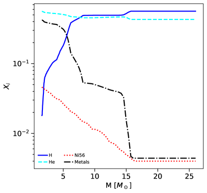
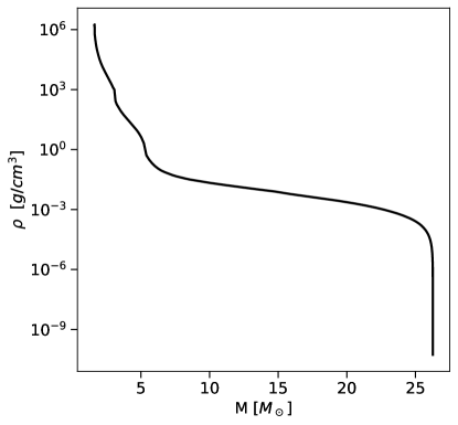
Figure 1: Left panel: The mass fraction of hydrogen (blue solid line), helium (cyan dashed line), heavy elements (black dash-dotted line), and radioactive ⁵⁶Ni (red dotted line) in the ejecta of the model M1 (the model which best reproduces the observed SN Refsdal light curves; see Section 3.1). Right panel: the density distribution of the model M1 as a function of interior mass. The total mass of the pre-supernova is $M_{tot}=26.3\,M_{\odot}$, $M_{{}^{56}\mathrm{Ni}}=0.25\,M_{\odot}$, the mixing is artificial. After an explosion, a core with a mass of $1.6\,M_{\odot}$ is left.

The explosion was triggered using the ‘‘thermal bomb’’ model (Shigeyama & Nomoto, 1990; Blinnikov et al., 2000), namely, via a short ($\Delta t_{burst}=0.1s$) release of thermal energy $E_{burst}$ in the near-central with the mass of $0.06M_{\odot}$ on the outer edge of the core with the mass of $M_{core}=1.6M_{\odot}$ (Blinnikov et al. (2000)). The core material forms a proto-neutron star and does not participate in the expansion of the supernova envelope. In the equations of motion of the envelope material, the contribution of the core to the gravitational potential is taken into account.

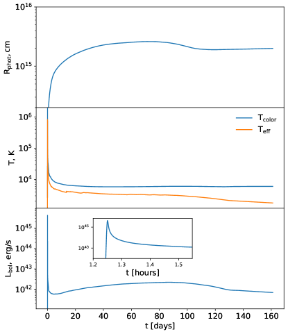
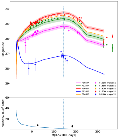
Figure 2: The observational properties of the best-fit model M1. The left panel shows the photospheric radius, the color and effective temperature, and the bolometric luminosity. shows the multi-band photometry for S1 image and the evolution of the photosphere velocity in comparison with H$\alpha$ expansion velocity measurements (black circle) from Kelly et al. 2016. Note that observed LCs in all filters are well-reproduced by M1, although for fitting we used only F160W, F125W, and F105W passbands (these filters are shown with the model uncertainties).

Table 1: The parameter space of our 185 SN models

	$R_{0}$ [$R_{\odot}$]	$M_{tot}$ [$M_{\odot}$]	$M_{{}^{56}\mathrm{Ni}}$ [$M_{\odot}$]	$E_{burst}$ [E51]	$Z$
min	$30$	$16$	$0.077$	$1$
	⋮	⋮	⋮	⋮	⋮
max	$100$	$27$	$0.42$	$7$

Table 2: the parameters of the best-fit model M1.

	$R_{0}$ [$R_{\odot}$]	$M_{tot}$ [$M_{\odot}$]	$M_{ej}$ [$M_{\odot}$]	$M_{{}^{56}\mathrm{Ni}}$ [$M_{\odot}$]	$E_{burst}$ [E51]	$Z$
	$50\pm 1$	$25\pm 2$	$23.4\pm 2$	$0.26\pm 0.05$	$4.7\pm 0.8$	$0.005\pm 0015$
Best-fit	$50$	$26.3$	$24.7$	$0.247$	$5$	$0.004$

To obtain the model which simultaneously reproduces multi-band SN Refsdal light curves, we computed set of 185 radiation-hydrodynamical models. SN Refsdal gravitationally lensed supernova, and the absolute magnifications of its images are poorly constrained. For example, the absolute magnification for S1 predicted by different lens models (Oguri, 2015; Kawamata et al., 2016; Sharon & Johnson, 2015; Jauzac et al., 2016; Grillo et al., 2016) is $\mu_{S1}\sim 10\div$. Thus, we use the observed peak luminosity as a constraint. Instead, we try to reproduce the shape of SN Refsdal light curves in different bands keeping in mind available in the literature estimates of the absolute magnifications for S1 and measured in Kelly et al. (2016) H$\alpha$ expansion velocity. The ranges of values of the SN models parameters are given in Table 1. Note that the parameters are not distributed uniformly in the parameter space, but converge to some optimal model (in the sense of Bayesian evidence, see Appendix A). At each time step, Stella calculates the spectral energy distributions (SEDs) which are then transformed from host galaxy rest-frame ($z=1.49$) into the observer’s frame and convolved with the transmission functions of the HST filters. Here, we use the F105W, F125W and F160W bands since the coverage of the Refsdal light curve in these bands is most complete and well-sampled.

3.1 Best-fit SN Refsdal model

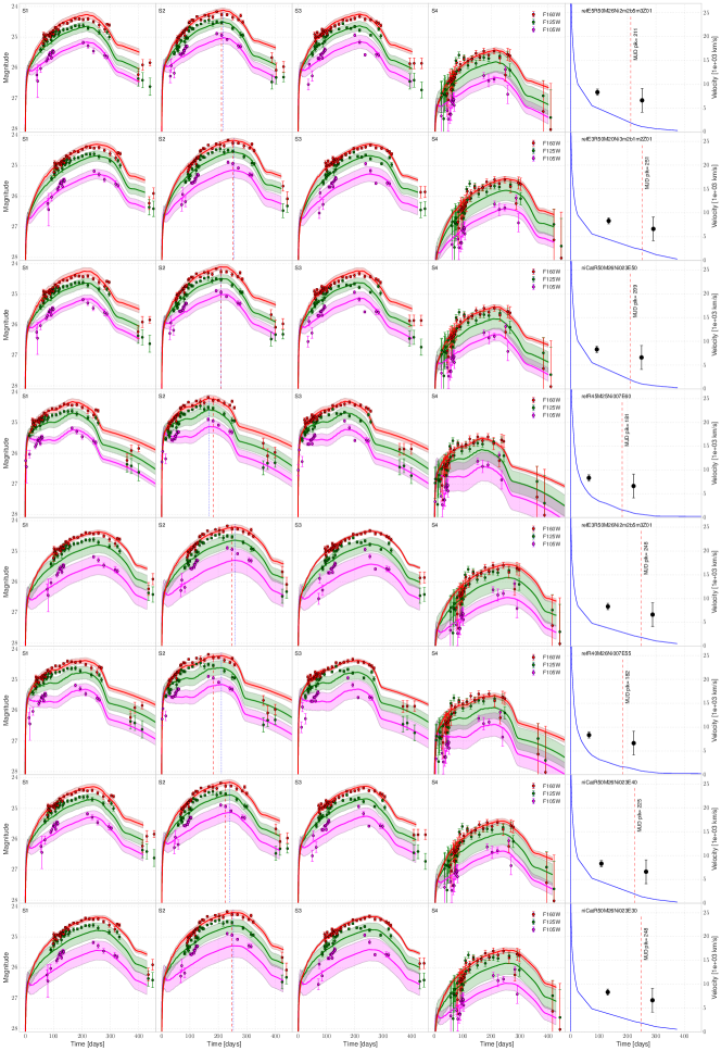
Figure 8: Light curves and the photosphere velocity evolution of the best-performing SN models listed in Table 4. The best-fit model M1 is shown in the first row, M2 is in the second, …, M8 is in the eighth row. In each row, the first four panels show the observed and model LCs for SN Refsdal images S1-S4 (from left to right). Shaded areas indicate the model uncertainties in each passband. The most right panel in each row plots the model photospheric velocity evolution in comparison with H$\alpha$-velocity measurements from Kelly et al. 2016. As expected, H$\alpha$-velocities are systematically higher than the photospheric velocities.

the best-fit model (as well as the time delays and magnification ratios) is described in detail in Appendix A. Here, we just outline the main steps. For each computed SN model, we compare synthetic LCs with observations and maximize the likelihood function (A1) with five free parameters: the absolute time and magnitude shifts for the reference image S1, and the model photometric uncertainties in three HST passbands used (see Appendix A for a discussion why model uncertainties are introduced as fit parameters). As the priors for all the fit parameters, we use uniform distributions spanning a wide range of values. Then we determine the time and magnitude shifts of images S2-S4 relative to S1 in a similar fashion. Next, we calculate the posterior probability of each SN model, and use the obtained value as a measure of how well the model fits observations. We report the 8 best-performing SN models in Table 4 and show the model light curves in comparison with observations in Figure 8.

The model M1 fits best to the observed SN Refsdal LCs, and the resulting photospheric velocity is in agreement with available H$\alpha$ expansion velocity measurements from Kelly et al. (2016). The photospheric velocity can be inferred from a blueshift of weak absorption lines such as the lines of FeII 5018Å and 5169Å. For SNe type IIP including peculiar 1987A-like SNe, the FeII lines show systematically lower velocities compared to H$\alpha$ (Blanco et al., 1987; Taddia et al., 2012). Therefore, H$\alpha$ velocities should be systematically higher than the photospheric velocities of our models.

The main parameters of the best-fit model M1 are the following: the total mass $M_{ej}=26.3\,M_{\odot}$, the ejecta mass $M_{ej}=24.7\,M_{\odot}$, the pre-SN radius $R_{0}=50\,R_{\odot}$, the ⁵⁶Ni mass $M_{{}^{56}\mathrm{Ni}}=0.25\,M_{\odot}$ and the explosion energy $E_{burst}=5\times 10^{51}$ ergs (listed in Table 2).

BSGs are compact, and the time of shock breakout is $\approx$ 1.25 hour with the boundary velocity of $\approx$ 59 000 km s^-1 (see Figure 2). Soon after the shock breakout at $t\approx$ 1.4 hour the radiative losses became small compared to the kinetic energy of the shell. Thus, internal temperature in the shell falls almost adiabatically, while the bolometric luminosity decreases to $7\times 10^{41}$ ergs/s and then reaches its local minimum at day 1 after the explosion (see Figure 2, left panel). Details of the explosion model (the duration of the energy release and the mass of the thermal bomb) majorly influence the magnitude and the shape of the first maximum of the light curve. For the SN Refsdal modeling, these parameters are relatively inessential, since observations started during the rise toward the second maximum of the light curve (cupola), which forms determined by properties of the cooling and recombination wave and contribution of radioactive ⁵⁶Ni decay.

Our $M_{{}^{56}\mathrm{Ni}}=0.25\,M_{\odot}$ estimate is within the range of $(0.005-0.28)M_{\odot}$ implied by the observed distribution of $M_{{}^{56}\mathrm{Ni}}$ for SN II (Müller et al., 2017) and consistent with the high energy of explosion (Sukhbold et al., 2016). Note that the total energy release in M1 is greater than $2\times 10^{51}$ erg, i.e. beyond the range implied by neutrino-driven explosions (Sukhbold et al., 2016). Sukhbold et al. (2016) found that at most 6-8% of the SN IIP explosions are connected to progenitors more massive than 20$M_{\odot}$when they used SN 1987A-calibrated neutrino engines. Nevertheless, M1 with $M_{ej}=24.7\,M_{\odot}$ is quite similar to other well-explored peculiar 1987a-like SNe, $M_{ej}>20\,M_{\odot}$ (Taddia et al., 2012).

Metallicity in the outer layers of the M1 envelope is reduced by the factor of ($Z_{M1}=$) relative to ($Z_{\odot}=0.02$) and is comparable with the value ($Z=0.005$) of the model by Nomoto & Hashimoto (1988). , the contribution of line opacity to the total opacity is significant. The line opacity drops dramatically from UV toward optical wavelengths. Thus, lower metallicity mainly affects the light curves in blue and UV light curves, what allowed us to reproduce the light curves in the F814W band (see Figure 2, right panel).

According to our best-fit model, the absolute magnification of S1 image is $\simeq 10$ (see column 8 of Table 5) which the range of magnifications $\mu_{S1}\sim 10\div\textbf{25}$ predicted by different lens models (Oguri, 2015; Kawamata et al., 2016; Sharon & Johnson, 2015; Jauzac et al., 2016; Grillo et al., 2016). To increase the absolute magnification of S1, we should reduce a radiated flux. The model M4 (see Table 4) has $M_{{}^{56}\mathrm{Ni}}=0.12\,M_{\odot}$ in the envelope, i.e. $\sim 2$ times less than the best-fit model. Thus, the amount of heat released as a result of ⁵⁶Ni decay is also $\sim 2$ times lower, and smaller amount of energy can be radiated. Figure 8 illustrates that M4 fits the SN Refsdal LCs if the absolute magnification of S1 is $\mu_{M4}=18.6$, i.e. $\sim 2$ times larger than for M1. In principle, the amount of ⁵⁶Ni and, as a consequence, the absolute magnification, can be constrained from spectral lines (Utrobin & Chugai, 2011) or by the slope of the tail of the supernova light curves (Nadyozhin, 2003).

4 Time delays and magnification ratios

4.1 SN Refsdal images S1-S4

In the previous Section, for each computed SN model we derived the best-fit absolute time and magnitude shifts for the image S1. By fitting the model light curves to images S2, S3, and S4, we obtained the time shifts and magnifications of images S2-S4 relative to S1 (for details, see Appendix A). Figure 3 illustrates the results of our time delay and magnification calculations for the best-fit model M1. Each panel shows the composite light curve from images S1–S4, after applying the time and magnitude shifts so that S2-S4 match the S1 light curve. The best-fit model light curves are overplotted as red (F160W filter), green (F125W) and magenta (F105W) lines with the shaded bands indicating the model uncertainty. The photometric model uncertainties in each filter for the best-fit model are provided in Appendix A, Table 4 (see the first row).

Table 3: Summary of time delay and magnification ratio measurements.

Parameter	BMA Mean	Template Fits	Fits
$\mathtt{MJD}_{pk}$	$57144^{+10}_{-10}$ d	$57138\pm 10$ d	$57132\pm 4$ d
$\Delta t_{S2-S1}$	$9.5^{+2.6}_{-2.7}$ d	$4\pm 4$ d	$7\pm 2$ d
$\Delta t_{S3-S1}$	$4.2^{+2.3}_{-2.3}$ d	$2\pm 5$ d	$0.6\pm 3$ d
$\Delta t_{S4-S1}$	$30^{+7.8}_{-8.2}$ d	$24\pm 7$ d	$27\pm 8$ d
$\Delta t_{SX-S1}$	$340^{+43}_{-52}$ d	—	—
$\mu_{S2/S1}$	$1.14^{+0.021}_{-0.020}$	$1.15\pm 0.05$	$1.17\pm 0.02$
$\mu_{S3/S1}$	$1.01^{+0.019}_{-0.018}$	$1.01\pm 0.04$	$1.00\pm 0.01$
$\mu_{S4/S1}$	$0.35^{+0.016}_{-0.015}$	$0.34\pm 0.02$	$0.38\pm 0.02$
$\mu_{SX/S1}$	$0.24^{+0.12}_{-0.07}$	—	—

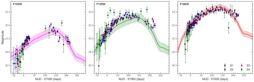
Figure 3: The composite light curves from images S1-S4 after applying the magnitude and time shifts (relative to the image S1) determined for the best-fit model M1. The best-fit model light curves are shown as solid lines with photometric uncertainties as shaded areas.

To derive a single measurement of the time delay and magnification ratio for SN images, that takes into account the Bayes factor and the uncertainty of each SN model, we use the (equations A4-A5). Mean values of time delays and magnification ratios obtained from the BMA combinations are provided in Table 3.

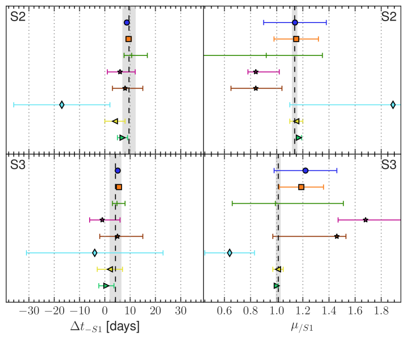
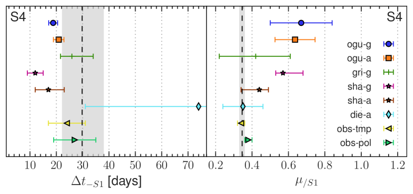
Figure 4: Comparison of lens model predictions with time delay and magnification values obtained in this work. The left and right columns present the time delays and magnification ratios (both relative to S1), correspondingly. Results for images S2, S3, and S4 are shown from top to bottom. The dashed vertical lines and the gray shaded regions indicate our best estimate of the time delay/magnification ratio with uncertainties (see column 2 in Table 3). Values predicted by different lens models (‘Die-a’,‘Gri-g’, ‘Ogu-a’, ‘Ogu-g’, ‘Sha-a’, ‘Sha-g’) are plotted as colored (see the legend in the lower right panel). Yellow and green triangles mark the measurements from Rodney et al. 2016 derived from light curve template (‘obs-tmp’) and polynomial (‘obs-pol’) fitting, correspondingly.

Thanks to the discovery of the first multiply-lensed supernova, the galaxy cluster MACS 1149.5+2223 has been extensively observed and modelled by several independent lens teams (see, e.g., Oguri, 2015; Kawamata et al., 2016; Sharon & Johnson, 2015; Grillo et al., 2016; Jauzac et al., 2016). Comparison of lens models and summary of the time delays and magnification ratios predicted by those models are given in Treu et al. (2016). Figure 4 presents a comparison of our measured mean time delays and magnification ratios for SN Refsdal images S1–S4 against the lens model predictions from Treu et al. (2016) (namely, ‘Die-a’,‘Gri-g’, ‘Ogu-a’, ‘Ogu-g’, ‘Sha-a’, ‘Sha-g’). from the template and polynomial fitting (Rodney et al., 2016) are also shown. Our with results of Rodney et al. (2016) (see Table 3).

4.2 SX

Approximately a year after the discovery of SN Refsdal ‘Einstein cross’, a fifth image appeared. As it was expected, SX is much fainter than S1-S4 and its photometric measurements are scarce. We repeat the procedure of maximizing the likelihood function (see Appendix A) to find the best-fit values of the time and magnitude shifts of SX relative to S1 for 8 best-fit SN models. The 8 best performing models are illustrated in Figure 9, and Figure 10 shows the marginal distributions for the SX-S1 time delay and the SX magnification for the best-fit model M1. The obtained marginalized distributions are quite broad (for all best performing models, not only for M1), and, as a consequence, uncertainties on the parameters of interest are large. Due to a broad peak the model light curves in F125W and F160w filters are relatively featureless, and 2-3 data points are not enough to obtain tight constraints.

We again calculate the mean values using the BMA method. The time delay and the magnification of SX are $\Delta t_{SX-S1}=340^{+43}_{-52}$ days, $\mu_{SX/S1}=0.24^{+0.12}_{-0.07}$. In Figure 5, we plot the best-fit model M1 and BMA estimates of the time delay and magnification ratio between images S1 and SX in comparison with the constraints from Kelly et al. (2016) and lens model predictions from several teams reported by Treu et al. (2016).

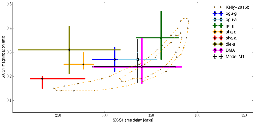
Figure 5: The best-fit model M1 and BMA constraints (in magenta) on the time delay and magnification of the image SX relative to S1. 1$\sigma$ and 2$\sigma$ orange contours show results from Kelly et al. 2016 where the shape of LC was obtained via fitting second-order polynomials to S1 measurements in F125W and F160W bands separately. Values predicted by different lens models are plotted as colored points (see the legend in the right corner).

5 Hubble constant

More than half a century ago Refsdal (1964) proposed to use time-delays between multiple images of gravitationally lensed supernovae to measure the Hubble constant. However, no multiply imaged SN has ever been observed until just recently. In practice, the strong lens time delay cosmography has been employed extremely successfully for decades using multiply imaged quasars. For example, the H0LiCOW collaboration (Suyu et al., 2017) has recently constrained $H_{0}$ to 2.4% precision for a flat $\Lambda$CDM cosmology from a joint analysis of six gravitationally lensed quasars with measured time delays (Wong et al., 2020). To achieve such a precision, one needs a variety of observational data. For example, to measure time delays between images several years of photometric monitoring of the lens system are typically required, because the light curves of quasars are stochastic and heterogeneous and their intrinsic stochasticity is hard to disentangle from variability due to microlensing (e.g., Eigenbrod et al., 2005; Tewes et al., 2013; Dobler et al., 2015, among others). In contrast to quasars, gravitationally lensed SNe with multiple images occur on short timescales, allowing their time delays to be measured with far less observational efforts. Moreover, after lensed SNe fade away, one can obtain imaging of a host galaxy to validate the lens model. In addition, the intrinsic luminosities of SN Ia and certain types of core-collapse SNe can be determined independently of lensing, which allows to directly measure the lensing magnification factor. A model-independent estimate of the magnification can improve constraints on the lens model especially for galaxy clusters with only few known multiple image systems (Riehm et al., 2011).

Here, we constrain the Hubble constant using the values of time delays between SN Refsdal images determined in Section 4. While modelling the SN Refsdal light curves and determining time delays between images, we have ignored the microlensing effect. A preliminary assessment of whether there are any indications of especially strong microlensing events that could bias time delay and magnification measurements is given in Rodney et al. (2016). They concluded that the SN Refsdal light curves are unlikely to be affected by major microlensing events. Throughout the paper, we assume that microlensing has no influence on our results but there are studies which show that microlensing does indeed introduce uncertainty in the time delay and the Hubble constant measurements (see, e.g., Dobler & Keeton, 2006; Goldstein et al., 2018; Pierel & Rodney, 2019). Huber et al. (2019); Suyu et al. (2020) discuss the best strategies to detect gravitationally lensed SNe and to measure their time delays with high accuracy in the presence of microlensing.

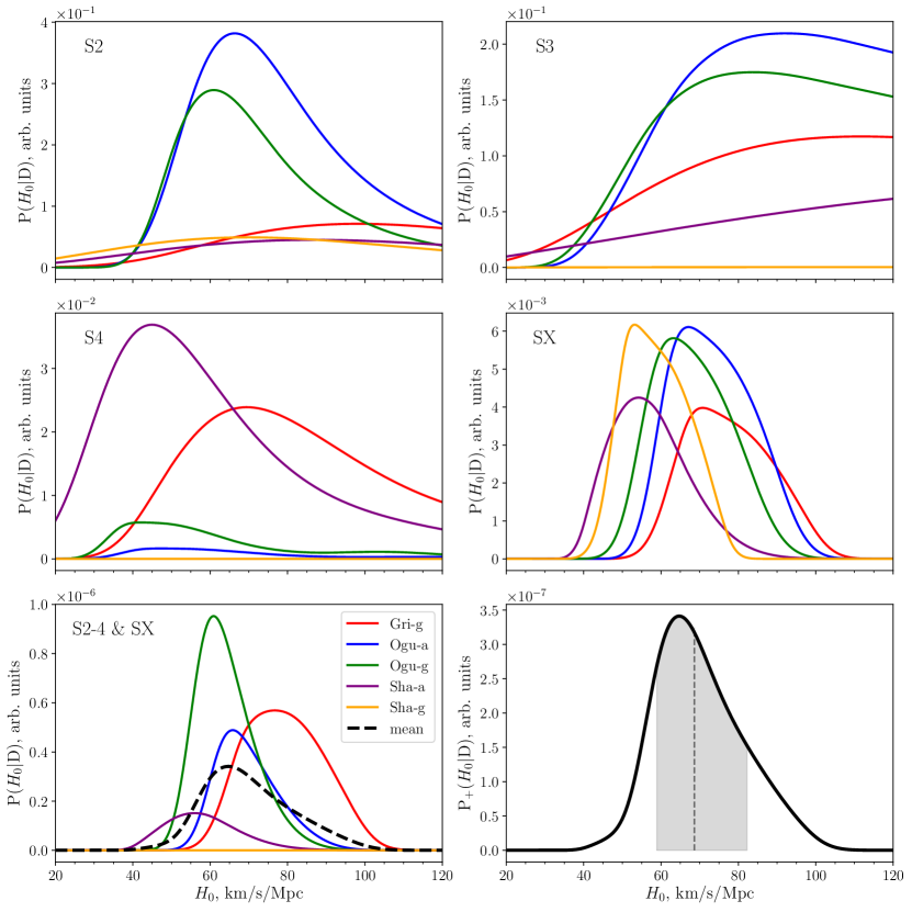
Figure 6: $P(D|H_{0})=\int p_{lens}(\Delta t|H_{0})\cdot p_{obs}(\Delta t)d\Delta t\,\times\int p_{lens}(\mu)\cdot p_{obs}(\mu)d\mu\,$ for different lens models calculated for images S2, S3, S4, and SX separately. Lens models are shown with different colors as indicated in the legend in the lower left panel. Lower left panel: contributions (from all images) of lens model predictions to the posterior distribution $\mathrm{P}_{+}(H_{0}|\mathrm{D})$, shown in the lower right panel. Lower right panel: The total posterior distribution $\mathrm{P}_{+}(H_{0}|\mathrm{D})$ defined as the mean of likelihood functions $P(D|H_{0})$ of different lens models. The dashed line marks the median value of $H_{0}$. The grey shaded area denotes the 16th and 84th percentile confidence band. The best value for $H_{0}$ resulting from the combined analysis of all images is $68.6^{+13.6}_{-9.7}$ km s^-1 Mpc^-1.

To derive $H_{0}$, we follow the approach proposed in Vega-Ferrero et al. (2018) where the Hubble constant is obtained via re-scaling the time delays predictions of the lens models to match the observed values (although, see Grillo et al. 2018 for discussion on possible caveats of this approach). The following lens models are considered here: ‘Gri-g’, ‘Ogu-g’, ’Ogu-a’, ’Sha-g’, and ’Sha-a’. Description of these models, time delays, and magnification predictions for all SN Refsdal images are given in Treu et al. 2016 (see their Table 6). Following Vega-Ferrero et al. (2018), we estimate the probability of $H_{0}$ given ‘observational’ data $\mathrm{D}$ ( obtained best-fit values of $\Delta t$ and $\mu$ listed in Table 3) as

$$\begin{split}\mathrm{P}(H_{0}|\mathrm{D})\propto\mathrm{P}(H_{0})\leavevmode\nobreak\ \mathrm{P}(\mathrm{D}|H_{0})\propto\\ \mathrm{P}(H_{0})\int d\Delta t\,d\mu\,\cdot p_{lens}(\Delta t,\mu|H_{0})\cdot p_{obs}(\Delta t,\mu),\end{split}$$ (1)

where $\mathrm{P}(H_{0})$ is the prior for $H_{0}$ (assumed to be flat between 20 and 120 km s^-1 Mpc^-1), $p_{lens}(\Delta t,\mu)$ is the distribution of time delay and magnification predictions of a given lens model (which can be re-scaled to any alternative value of $H_{0}$), and $p_{obs}(\Delta t,\mu)$ is the ‘observational’ distribution obtained in this work. We assume that for each lens model, $p_{lens}(\Delta t,\mu$) is described with a normal bivariate distribution (with no correlation between $\Delta t$ and $\mu$). The mean values and their statistical uncertainties for each image are taken from Table 6 of Treu et al. (2016). To obtain the ‘observed’ distributions $p_{obs}(\Delta t)$ and $p_{obs}(\mu)$, we average marginalized distributions of all explored SN models using the BMA method with weights corresponding to posterior probabilities of SN models (see Appendix A). Figure 6 shows the obtained $P(\mathrm{D}|H_{0})$ for different lens models for each image separately (upper and middle panels) and the ‘combined’ $P(\mathrm{D}|H_{0})$ distributions (lower left panel) calculated as a product of $P(\mathrm{D}|H_{0})$ for separate images. The total posterior distribution $\mathrm{P}_{+}(H_{0}|\mathrm{D})$ (see the lower right panel of Figure 6) is calculated as the mean of ‘combined’ $P(\mathrm{D}|H_{0})$ distributions for lens models. The median value and 68% for the Hubble constant are $68.6^{+13.6}_{-9.7}$ km s^-1 Mpc^-1. We see that the lens models ‘Ogu-g’, ‘Ogu-a’, and ‘Gri-g’ contribute most to the total $\mathrm{P}_{+}(H_{0}|\mathrm{D})$, i.e. these models are in a good agreement with time delays and magnification ratios obtained in this work.

With more photometric measurements of image SX , we will be able to drastically improve our time delay and magnification measurements as well as accuracy of $H_{0}$ determination.

6 Conclusions

Hydrodynamic simulation of the light curves and the expansion velocities us to get significant insights into the nature of core-collapse SN progenitors, namely, to estimate radius and mass of a progenitor star, an explosion energy, an ejecta mass, and a radioactive ⁵⁶Ni amount. At high redshifts, core-collapse supernovae, especially Type IIP, are hard to discover due to their faintness. The highest-redshift spectroscopically confirmed SN IIP is PS1-13bni with redshift of $z=0.335^{+0.009}_{-0.012}$ (Gall et al., 2018). With the help of gravitational lensing, we can probe SN IIP at much greater distances. Before discovery of SN Refsdal, the highest redshift core-collapse SN (most likely Type IIP) was at $z\simeq 0.6$ (Stanishev et al., 2009). This transient was found in the Abell 1689 galaxy cluster and probably was magnified by $\sim 1.4$ mag. Unfortunately, its light curve is poorly sampled to perform a detailed analysis. discovery of SN Refsdal offered us a unique opportunity to model such a distant supernova ($z=1.5$) and to study properties of its progenitor. We modelled SN Refsdal using the multi-group radiation-hydrodynamics numerical code Stella which allows one to construct synthetic light curves in various photometric bands and for the expansion velocity of the H$\alpha$ shell. For the first time, we obtained the hydrodynamic model of a SN IIP at a cosmologically relevant distance. We computed a set of 185 hydrodynamical models covering a rather large area in the parameter space. We confirm the conclusion of Kelly et al. (2016) that SN Refsdal is a more energetic version of SN 1987A.

Future deep surveys should be able to detect large number of gravitationally lensed supernovae, including Type IIP, at high redshifts. Analysis of their light curves should allow us to compare high-$z$ SNe with the local IIP population to investigate any systematic difference between high and low redshift SNe.

Proper reconstruction of SN Refsdal light curve allowed us relative time delays and magnification ratios between images S2-S4 and S1. Mean values (obtained via Bayesian Averaging Method) with uncertainties are provided in Table 3. We anticipated that we would be able to constrain the time delay of the fifth SN Refsdal image SX and its magnification relative to S1 with an accuracy of several percent. Unfortunately, quite a broad ‘featureless’ peak of the light curve combined with very scarce photometric measurements for SX resulted in large uncertainties for parameters of interest. We obtain (again, using BMA method) $\Delta t_{SX-S1}=340^{+43}_{-52}$ days and $\mu_{SX/S1}=0.24^{+0.12}_{-0.07}$. Following approach suggested in Vega-Ferrero et al. (2018), we computed the Hubble constant $H_{0}=68.6^{+13.6}_{-9.7}$ km s^-1 Mpc^-1 via re-scaling the time predictions of the lens models to match the values obtained in this work. With more photometric data on SX, accuracy of $H_{0}$ determination can be drastically improved.

Appendix A Fitting model light curves to observations

Here, we describe our approach of fitting synthetic light curves to observations. As discussed in Section 3, we constructed a set of 185 hydrodynamic SN models to find the optimal model which interprets simultaneously available photometric and spectroscopic observations of SN Refsdal. Namely, we use well-sampled measurements in the F160W, F125W and F105W bands and H$\alpha$ velocities as constraints. For each SN model, we derive the logarithmic likelihood function (A1):

$$\log L\left(m^{o}|m^{m},\Theta\right)=-\frac{1}{2}\sum_{S,t}\left[\frac{\left(m_{S}^{o}(t)-m_{S}^{m}(t+\Delta t)-\Delta m\right)^{2}}{\sigma_{S}^{2}}+\log(2\pi\sigma_{S}^{2})\right],$$ (A1)

where $m_{S}^{m}(t)$ is the light curve in a given filter $S$ ($S$ = F160W, F125W or F105W), $m_{S}^{o}(t)$ is the observed light curve in a filter $S$ sampled at time instances $t$, the total uncertainties $\sigma_{S}^{2}=\sigma_{o}^{2}+\sigma_{m}^{2}$ are represented with two components: the observational photometric uncertainties $\sigma_{o}$ and the model uncertainties $\sigma_{m}$. Summation is done over three HST filters and time instances at which observations are available. Vector $\Theta$ denotes the set of five free parameters - the time shift $\Delta t$, $\Delta m$ and the model uncertainties $\sigma_{m}$ for F105W, F125W, F160W filters - which we determine for each SN model by maximizing the log-likelihood (A1). Since Stella allows one to calculate light curves in multiple bands self-consistently, to match observations we shift all synthetic light curves in brightness by a single value of $\Delta m$ without adding any filter-related corrections. Unfortunately, the ‘true’ model uncertainties are hard to evaluate. Moreover, Stella is 1D and makes several simplifying assumptions to numerically treat the radiation hydrodynamics. Thus, the perfect fit of a model to observations does not necessarily leads one to the ‘true’ physical parameters. It’s more important that the model captures correctly the general shape of the observed LCs. That’s why we artificially introduced the model uncertainties for each band as fitting parameters. Such an approach also allows us to assign (implicitly) different weights to observations in different bands. For example, as can be seen from Table 4 the best-fit model uncertainty for filter F105W is always larger than $\sigma_{m}$ for F160W. This is partly due to the fact that data in filter F105W are much more sparse and with larger error bars than measurements in F160W.

Having the absolute $\Delta t$ and $\Delta m$ of image S1 fixed, we fit the model light curves to images S2, S3, S4, and SX by maximizing the function (A1) with five free parameters: the time delay of a considered image relative to S1, the magnitude shift relative to S1 and the model uncertainties for three considered HST filters.

The likelihood distributions are sampled using the Markov Chain Monte Carlo ensemble sampling tools from the emcee software package (Foreman-Mackey et al., 2013).

Next, we derive the model evidence (the marginal distributions of the observations $D$ given the SN model $M_{l}$ averaged over the prior distributions of all the parameters constituting the vector $\Theta$):

$$\pi(D|M_{l})=\sum_{i}L(\Theta_{i})Pr(\Theta_{i})$$ (A2)

Then we define the posterior probability of each SN model given observations as:

$$\pi(M_{l}|D)=\frac{\pi(D|M_{l})\pi(M_{l})}{\sum_{m}\pi(D|M_{m})\pi(M_{m})},$$ (A3)

where we sum up over all 185 SN models in the denominator to ensure that the cumulative posterior probability over all models equals unity. Obtained posterior probabilities $\pi(M_{l}|D)$ can be used as a straightforward model selection criteria (Hoeting et al., 1999), with the most likely model having the highest value of $\pi(M_{l}|D)$.

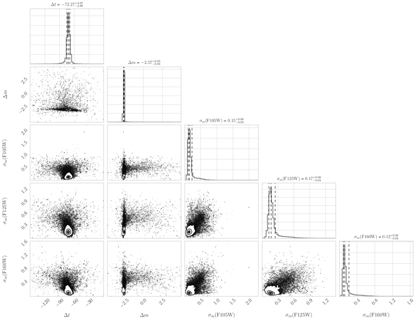
Figure 7: The MCMC corner plot for the best-fit model M1 showing 1D and 2D marginalized probability contours for each of the five fit parameters (the absolute time shift and of image S1, and the model uncertainties in three passbands). The histograms on the diagonal also include the positions of the 16th, 50th, and 84th percentiles.

Table 4: Parameters of the 8 best performing SN models

Model	$\pi(M_{l}|D)$	$\Delta t$	$\Delta m$	$\sigma_{m}(F160W)$	$\sigma_{m}(F125W)$	$\sigma_{m}(F105W)$	$R_{0}$	$M_{tot}$	$M_{{}^{56}\mathrm{Ni}}$	$E_{burst}$
		(days)					($R_{\odot}$)	($M_{\odot}$)	($M_{\odot}$)	(E51)
M1	0.711	${-72}^{+2.6}_{-2.2}$	${-2.57}^{+0.024}_{-0.029}$	${0.11}^{+0.03}_{-0.02}$	${0.16}^{+0.04}_{-0.03}$	${0.14}^{+0.04}_{-0.03}$	50.0	26.3	0.25	5.0
M2	0.165	${-111}^{+2.7}_{-2.7}$	${-2.18}^{+0.027}_{-0.047}$	${0.10}^{+0.05}_{-0.03}$	${0.17}^{+0.05}_{-0.05}$	${0.16}^{+0.05}_{-0.04}$	50.0	20.6	0.37	3.0
M3	0.088	${-71}^{+2.4}_{-2.5}$	${-2.57}^{+0.025}_{-0.028}$	${0.12}^{+0.03}_{-0.02}$	${0.16}^{+0.04}_{-0.03}$	${0.13}^{+0.04}_{-0.03}$	50.0	26.0	0.24	5.0
M4	0.0258	${-33}^{+0.4}_{-0.4}$	${-3.17}^{+0.017}_{-0.017}$	${0.10}^{+0.02}_{-0.02}$	${0.17}^{+0.03}_{-0.03}$	${0.11}^{+0.04}_{-0.03}$	45.0	25.0	0.12	6.0
M5	0.0047	${-109}^{+2.8}_{-4.5}$	${-2.58}^{+0.018}_{-0.028}$	${0.06}^{+0.03}_{-0.02}$	${0.25}^{+0.05}_{-0.05}$	${0.31}^{+0.07}_{-0.07}$	50.0	26.3	0.24	3.0
M6	0.0022	${-45}^{+3.3}_{-2.4}$	${-3.22}^{+0.020}_{-0.022}$	${0.09}^{+0.02}_{-0.02}$	${0.21}^{+0.04}_{-0.03}$	${0.19}^{+0.05}_{-0.04}$	40.0	26.0	0.12	5.5
M7	0.0021	${-87}^{+3.2}_{-3.7}$	${-2.57}^{+0.027}_{-0.062}$	${0.10}^{+0.07}_{-0.03}$	${0.19}^{+0.05}_{-0.06}$	${0.21}^{+0.05}_{-0.06}$	50.0	26.0	0.24	4.0
M8	0.0012	${-108}^{+3.3}_{-5.1}$	${-2.59}^{+0.020}_{-0.035}$	${0.07}^{+0.04}_{-0.02}$	${0.25}^{+0.05}_{-0.06}$	${0.31}^{+0.07}_{-0.08}$	50.0	26.0	0.24	3.0

For each SN model in our set, we evaluate $\pi(M_{l}|D)$ by comparing the synthetic light curves with observations for SN Refsdal images S1-S4 in F105W, F125W, F160W pass bands. As a result, for each SN model we obtain $\pi(M_{l}|D)$ and the best-fitting parameters: the absolute time shift of image S1, i.e. modified Julian date of the explosion (MJD_exp), and the absolute magnification of S1 (both of which are actually nuisance parameters), the time shifts of images S2-S4 relative to S1 and magnification ratios. Table 4 lists the best-fit parameters for S1 (the absolute time shift $\Delta t$, the absolute magnitude shift $\Delta m$, and the model uncertainties $\sigma_{m}$ for F105W, F125W, F160W filters) as well as the basic SN model characteristics for 8 best performing models. Note that the best-fit absolute magnifications of S1 $\mu=10^{-\Delta m/2.5}\simeq 7.5\div 20$ for SN models in Table 4 absolute magnifications predicted by lens models (Oguri, 2015; Kawamata et al., 2016; Sharon & Johnson, 2015; Jauzac et al., 2016; Grillo et al., 2016). This is not a result of fine-tuning since for $\Delta m$ determination we used a flat prior in a wide range of values $\Delta m\in$ (-5, 5). Table 5 shows relative time delays for images S2-S4 in days, magnification ratios as well as the explosion and peak MJDs. Despite the fact that for the top three SN models (the first three rows in Table 5) the explosion dates (or the absolute time shift in Table 4) vary noticeably, the resulting relative time delays are not that different. similar conclusion can be made about magnifications. The absolute magnification varies at most by a factor of $\sim 2.5$, while the relative magnifications (columns 9-11 in Table 5) show variations by several percent only. Table 4 also provides values of $\pi(M_{l}|D)$ for each model which reflect quality of fit to the data. The best-fit model M1 (see Table 4) significantly outperforms all the others (what is not surprising since it was our goal to construct the SN model which matches best available SN Refsdal observations). For the best-fit model, Figure 7 plots 2D and 1D probability distributions of each of the five fit parameters.

Table 5: Time delay and magnification measurements for SN Refsdal images S1-S4.

Model	$\pi(M_{l}|D)$	$\text{MJD}_{exp}$	$\text{MJD}_{pk}$	$\Delta t_{S2-S1}$	$\Delta t_{S3-S1}$	$\Delta t_{S4-S1}$	$\mu_{S1}$	$\mu_{S2/S1}$	$\mu_{S3/S1}$	$\mu_{S4/S1}$
$M1$	$0.711$	$56928^{+2.57}_{-2.23}$	$57145^{+2.6}_{-2.2}$	$10.0^{+1.93}_{-2.04}$	$4.2^{+2.35}_{-2.34}$	$30.4^{+6.59}_{-8.00}$	$10.62^{+0.285}_{-0.229}$	$1.14^{+0.019}_{-0.019}$	$1.01^{+0.019}_{-0.018}$	$0.34^{+0.015}_{-0.014}$
$M2$	$0.165$	$56889^{+2.70}_{-2.79}$	$57141^{+2.7}_{-2.8}$	$8.7^{+2.43}_{-2.45}$	$4.5^{+1.82}_{-1.97}$	$31.0^{+9.28}_{-7.81}$	$7.43^{+0.327}_{-0.176}$	$1.12^{+0.019}_{-0.019}$	$1.01^{+0.015}_{-0.014}$	$0.35^{+0.019}_{-0.015}$
$M3$	$0.088$	$56929^{+2.37}_{-2.47}$	$57138^{+2.4}_{-2.5}$	$11.2^{+1.86}_{-2.44}$	$4.7^{+2.62}_{-2.54}$	$28.7^{+6.70}_{-4.62}$	$10.71^{+0.283}_{-0.248}$	$1.14^{+0.020}_{-0.020}$	$1.01^{+0.020}_{-0.019}$	$0.34^{+0.013}_{-0.012}$
$M4$	$0.0258$	$56967^{+0.37}_{-0.45}$	$57134^{+0.4}_{-0.4}$	$0.5^{+0.28}_{-0.38}$	$0.5^{+0.28}_{-0.40}$	$12.2^{+1.04}_{-1.91}$	$18.59^{+0.302}_{-0.292}$	$1.11^{+0.018}_{-0.019}$	$1.01^{+0.016}_{-0.016}$	$0.33^{+0.010}_{-0.010}$
$M5$	$0.0047$	$56891^{+2.95}_{-5.49}$	$57150^{+3.0}_{-5.5}$	$9.4^{+3.20}_{-3.61}$	$4.7^{+1.85}_{-1.93}$	$34.0^{+10.84}_{-10.04}$	$10.74^{+0.403}_{-0.186}$	$1.15^{+0.024}_{-0.022}$	$1.03^{+0.013}_{-0.013}$	$0.38^{+0.024}_{-0.019}$
$M6$	$0.0022$	$56955^{+3.26}_{-2.48}$	$57166^{+3.3}_{-2.5}$	$12.0^{+0.54}_{-0.92}$	$1.0^{+1.38}_{-1.83}$	$20.5^{+3.32}_{-5.66}$	$19.41^{+0.388}_{-0.345}$	$1.15^{+0.019}_{-0.018}$	$1.00^{+0.013}_{-0.013}$	$0.35^{+0.013}_{-0.013}$
$M7$	$0.0021$	$56913^{+3.23}_{-3.72}$	$57152^{+3.2}_{-3.7}$	$10.7^{+2.85}_{-3.23}$	$5.3^{+2.62}_{-2.61}$	$33.1^{+7.55}_{-7.27}$	$10.69^{+0.648}_{-0.265}$	$1.14^{+0.022}_{-0.021}$	$1.02^{+0.019}_{-0.017}$	$0.36^{+0.016}_{-0.015}$
$M8$	$0.0012$	$56892^{+3.12}_{-4.66}$	$57145^{+3.1}_{-4.7}$	$8.8^{+3.30}_{-3.34}$	$4.9^{+2.26}_{-2.34}$	$32.4^{+11.35}_{-10.21}$	$10.81^{+0.344}_{-0.192}$	$1.15^{+0.023}_{-0.022}$	$1.03^{+0.014}_{-0.014}$	$0.37^{+0.024}_{-0.018}$
BMA	—	$56922^{+18.6}_{-18.6}$	$57144^{+10}_{-10}$	$9.5^{+2.6}_{-2.7}$	$4.2^{+2.3}_{-2.3}$	$30^{+7.8}_{-8.2}$	$10.2^{+1.9}_{-1.6}$	$1.14^{+0.021}_{-0.020}$	$1.01^{+0.019}_{-0.018}$	$0.35^{+0.016}_{-0.015}$

We compute a weighted average and an uncertainty of parameters of interest $\Theta$ across the explored set of SN models $M_{l}$ using the Bayesian Model Averaging approach (Hoeting et al., 1999):

$$E[\Theta]=\sum_{l}\pi(M_{l}|D)\;\Theta_{l}$$ (A4)

$$Var[\Theta]=\left|\sum_{l}\pi(M_{l}|D)\left(Var(\Theta_{l})+\Theta^{2}\right)-E[\Theta]^{2}\right|$$ (A5)

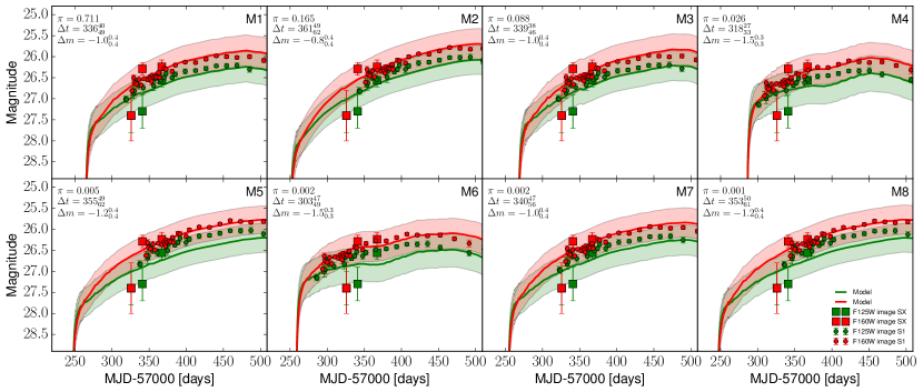
Figure 9: The model light curves of 8 best performing models fitted to the SX data (shows as squares). For comparison, S1 data are overplotted as circles.

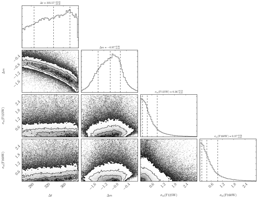
Figure 10: The MCMC corner plot for the best-fit model M1 showing marginal distributions for the following fit parameters: the SX-S1 time delay, the absolute magnitude shift for SX (which can be related to the magnification ratio as $\mu_{SX/S1}=10^{-dm/2.5}/\mu_{S1}$, where $\mu_{S1}$=10.62 is the absolute magnification for S1) and the model uncertainties in F125W and F160W filters. Dashed vertical lines in the histograms on the diagonal mark the positions of the 16th, 50th, and 84th percentiles.

The same procedure of finding the best-fit time and magnitudes shits is applied to SN Refsdal image SX.

The best performing models are shown in Figure 9. The marginal distributions of fit parameters for the best-fit model M1 are illustrated in Figure 10. The final time delay and magnification ratio estimates for SX (relative to S1) are obtained again via Bayesian Model Averaging and provided in Section 4.2.

References

- Baklanov et al. (2005) Baklanov, P. V., Blinnikov, S. I., & Pavlyuk, N. N. 2005, Astronomy Letters, 31, 429
- Baklanov et al. (2013) Baklanov, P. V., Blinnikov, S. I., Potashov, M. S., & Dolgov, a. D. 2013, JETP Letters, 98, 432
- Baklanov et al. (2015) Baklanov, P. V., Sorokina, E. I., & Blinnikov, S. I. 2015, Astronomy Letters, 41, 95
- Baron et al. (2004) Baron, E., Nugent, P. E., Branch, D., & Hauschildt, P. H. 2004, ApJ, 616, L91
- Bartunov et al. (1987) Bartunov, O. S., Blinnikov, S., Levakhina, L. V., & Nadezhin, D. 1987, Soviet Astronomy Letters, 13, 313
- Birrer et al. (2016) Birrer, S., Amara, A., & Refregier, A. 2016, Journal of Cosmology and Astroparticle Physics, 2016, 020
- Blanco et al. (1987) Blanco, W. M., Gregory, B., Hamuy, M., et al. 1987, ApJ, 320, 589
- Blinnikov & Sorokina (2004) Blinnikov, S., & Sorokina, E. 2004, Ap&SS, 290, 13
- Blinnikov et al. (2000) Blinnikov, S. I., Lundqvist, P., Bartunov, O. S., Nomoto, K., & Iwamoto, K. 2000, ApJ, 532, 1132
- Blinnikov et al. (2006) Blinnikov, S. I., Röpke, F. K., Sorokina, E. I., et al. 2006, A&A, 453, 229
- Chen et al. (2020) Chen, K.-J., Woosley, S. E., & Whalen, D. J. 2020, ApJ, 893, 99
- Cooke et al. (2012) Cooke, J., Sullivan, M., Gal-Yam, A., et al. 2012, Nature, 491, 228
- Dobler et al. (2015) Dobler, G., Fassnacht, C. D., Treu, T., et al. 2015, ApJ, 799, 168
- Dobler & Keeton (2006) Dobler, G., & Keeton, C. R. 2006, ApJ, 13
- Eastman & Pinto (1993) Eastman, R. G., & Pinto, P. A. 1993, ApJ, 412, 731
- Eigenbrod et al. (2005) Eigenbrod, A., Courbin, F., Vuissoz, C., et al. 2005, A&A, 436, 25
- Foreman-Mackey et al. (2013) Foreman-Mackey, D., Hogg, D. W., Lang, D., & Goodman, J. 2013, Publications of the Astronomical Society of the Pacific, 125, 306
- Gall et al. (2018) Gall, E. E. E., Kotak, R., Leibundgut, B., et al. 2018, A&A, 611, A25
- Goldstein et al. (2018) Goldstein, D. A., Nugent, P. E., Kasen, D. N., & Collett, T. E. 2018, ApJ, 855, 22
- Goobar et al. (2017) Goobar, A., Amanullah, R., Kulkarni, S. R., et al. 2017, Science, 356, 291
- Grillo et al. (2020) Grillo, C., Rosati, P., Suyu, S. H., et al. 2020, ApJ, 898, 87
- Grillo et al. (2016) Grillo, C., Karman, W., Suyu, S. H., et al. 2016, ApJ, 822, 78
- Grillo et al. (2018) Grillo, C., Rosati, P., Suyu, S. H., et al. 2018, ApJ, 860, 94
- Hillebrandt et al. (1987) Hillebrandt, W., Höflich, P., Truran, J. W., & Weiss, A. 1987, Nature, 327, 597
- Hoeting et al. (1999) Hoeting, J. A., Madigan, D., Raftery, A. E., & Volinsky, C. T. 1999, Statistical Science, 14, 382
- Huber et al. (2019) Huber, S., Suyu, S. H., Noebauer, U. M., et al. 2019, A&A, 631, A161
- Hunter (2007) Hunter, J. D. 2007, Computing in Science & Engineering, 9, 90
- Jauzac et al. (2016) Jauzac, M., Richard, J., Limousin, M., et al. 2016, MNRAS, 457, 2029
- Kawamata et al. (2016) Kawamata, R., Oguri, M., Ishigaki, M., Shimasaku, K., & Ouchi, M. 2016, ApJ, 819, 114
- Kelly et al. (2015) Kelly, P. L., Rodney, S. A., Treu, T., et al. 2015, Science, 347, 1123
- Kelly et al. (2016) Kelly, P. L., Brammer, G., Selsing, J., et al. 2016, ApJ, 831, 205
- Kelly et al. (2016) Kelly, P. L., Rodney, S. A., Treu, T., et al. 2016, ApJ, 819, L8
- Kirshner & Kwan (1974) Kirshner, R. P., & Kwan, J. 1974, ApJ, 193, 27
- Kochanek (2002) Kochanek, C. S. 2002, ApJ, 578, 25
- Kumagai et al. (1989) Kumagai, S., Shigeyama, T., Nomoto, K., et al. 1989, ApJ, 345, 412. http://adsabs.harvard.edu/doi/10.1086/167915
- Larchenkova et al. (2011) Larchenkova, T. I., Lutovinov, A. A., & Lyskova, N. S. 2011, Astronomy Letters, 37, 233
- Linder (2011) Linder, E. V. 2011, Phys. Rev. D, 84, 123529
- Lotz et al. (2017) Lotz, J. M., Koekemoer, A., Coe, D., et al. 2017, ApJ, 837, 97
- McCray & Fransson (2016) McCray, R., & Fransson, C. 2016, Annual Review of Astronomy and Astrophysics, 54, 19
- Menon et al. (2019) Menon, A., Utrobin, V., & Heger, A. 2019, MNRAS, 482, 438
- Müller et al. (2017) Müller, T., Prieto, J. L., Pejcha, O., & Clocchiatti, A. 2017, ApJ, 841, 127
- Nadyozhin (2003) Nadyozhin, D. 2003, MNRAS, 346, 97
- Nomoto & Hashimoto (1988) Nomoto, K., & Hashimoto, M.-A. 1988, Physics Reports, 163, 13
- Nugent & Hamuy (2017) Nugent, P., & Hamuy, M. 2017, in Handbook of Supernovae (Cham: Springer International Publishing), 2671–2688
- Nugent & Hamuy (2017) Nugent, P., & Hamuy, M. 2017, Cosmology with Type IIP Supernovae, ed. A. W. Alsabti & P. Murdin, 2671
- Oguri (2015) Oguri, M. 2015, MNRAS: Letters, 449, L86
- Oguri & Kawano (2003) Oguri, M., & Kawano, Y. 2003, MNRAS, 338, L25
- Perlmutter et al. (1999) Perlmutter, S., Aldering, G., Goldhaber, G., et al. 1999, ApJ, 517, 565
- Pierel & Rodney (2019) Pierel, J. D. R., & Rodney, S. 2019, ApJ, 876, 107
- Potashov et al. (2013) Potashov, M., Blinnikov, S. I., Baklanov, P. V., & Dolgov, A. 2013, MNRAS: Letters, 431, L98
- Refsdal (1964) Refsdal, S. 1964, MNRAS, 128, 307
- Riehm et al. (2011) Riehm, T., Mörtsell, E., Goobar, A., et al. 2011, A&A, 536, A94
- Riess et al. (1998) Riess, A. G., Filippenko, A. V., Challis, P., et al. 1998, AJ, 116, 1009
- Rodney et al. (2016) Rodney, S. A., Strolger, L. G., Kelly, P. L., et al. 2016, ApJ, 820, 50
- Sahu et al. (2008) Sahu, D. K., Tanaka, M., Anupama, G. C., et al. 2008, ApJ, 680, 580
- Saio et al. (1988) Saio, H., Nomoto, K., & Kato, M. 1988, Nature, 334, 508
- Sharon & Johnson (2015) Sharon, K., & Johnson, T. L. 2015, ApJ, 800, L26
- Sharon & Johnson (2015) Sharon, K., & Johnson, T. L. 2015, ApJ, 800, L26
- Shigeyama & Nomoto (1990) Shigeyama, T., & Nomoto, K. 1990, ApJ, 360, 242
- Sorokina et al. (2016) Sorokina, E., Blinnikov, S., Nomoto, K., Quimby, R., & Tolstov, A. 2016, ApJ, 829, 17
- Stanishev et al. (2009) Stanishev, V., Goobar, A., Paech, K., et al. 2009, A&A, 507, 61
- Sukhbold et al. (2016) Sukhbold, T., Ertl, T., Woosley, S. E., Brown, J. M., & Janka, H.-T. 2016, ApJ, 821, 38
- Suyu et al. (2017) Suyu, S. H., Bonvin, V., Courbin, F., et al. 2017, MNRAS, 468, 2590
- Suyu et al. (2020) Suyu, S. H., Huber, S., Cañameras, R., et al. 2020, arXiv e-prints, arXiv:2002.08378
- Taddia et al. (2012) Taddia, F., Stritzinger, M. D., Sollerman, J., et al. 2012, A&A, 537, A140
- Tewes et al. (2013) Tewes, M., Courbin, F., Meylan, G., et al. 2013, A&A, 556, A22
- Tominaga et al. (2011) Tominaga, N., Morokuma, T., Blinnikov, S. I., et al. 2011, ApJS, 193, 20
- Treu et al. (2016) Treu, T., Brammer, G., Diego, J. M., et al. 2016, ApJ, 817, 60
- Tsvetkov et al. (2019) Tsvetkov, D. Y., Baklanov, P. V., Potashov, M. S., et al. 2019, MNRAS, 487, 3001
- Utrobin (2005) Utrobin, V. P. 2005, Astronomy Letters, 31, 806
- Utrobin & Chugai (2011) Utrobin, V. P., & Chugai, N. N. 2011, A&A, 532, A100
- Vega-Ferrero et al. (2018) Vega-Ferrero, J., Diego, J. M., Miranda, V., & Bernstein, G. M. 2018, ApJ, 853, L31
- Wong et al. (2020) Wong, K. C., Suyu, S. H., Chen, G. C.-F., et al. 2020, MNRAS, 498, 1420
- Woosley et al. (2007a) Woosley, S. E., Blinnikov, S., & Heger, A. 2007a, Nature, 450, 390
- Woosley et al. (2007b) Woosley, S. E., Kasen, D., Blinnikov, S., & Sorokina, E. 2007b, ApJ, 662, 487
- Xu et al. (2016) Xu, D., Sluse, D., Schneider, P., et al. 2016, MNRAS, 456, 739