Flat-band ferromagnetism in twisted bilayer graphene

Abstract

We discuss twisted bilayer graphene (TBG) based on a theorem of flat band ferromagnetism put forward by Mielke and Tasaki. According to this theorem, ferromagnetism occurs if the single particle density matrix of the flat band states is irreducible and we argue that this result can be applied to the quasi-flat bands of TBG that emerge around the charge-neutrality point for twist angles around the magic angle $\theta\sim 1.05^{\circ}$. We show that the density matrix is irreducible in this case, thus predicting a ferromagnetic ground state for neutral TBG ($n=0$). We then show that the theorem can also be applied only to the flat conduction or valence bands, if the substrate induces a single-particle gap at charge neutrality. Also in this case, the corresponding density matrix turns out to be irreducible, leading to ferromagnetism at half filling ($n=\pm 2$).

I Introduction

Twisted bilayer graphene (TBG) has attracted much attention due to the recent discovery of superconductivity.Cao et al. (2018a); Yankowitz et al. (2019); Moriyama et al. ; Codecido et al. (2019); Shen et al. ; Lu et al. (2019); Chen et al. (2019); Xu and Balents (2018); Volovik (2018); Yuan and Fu (2018); Po et al. ; Roy and Juričić (2019); Guo et al. (2018); Dodaro et al. (2018); Baskaran ; Liu et al. (2018); Slagle and Kim (2019); Peltonen et al. (2018); Kennes et al. (2018); Koshino et al. (2018); Kang and Vafek (2018); Isobe et al. (2018); You and Vishwanath (2019); Wu et al. (2018); Zhang et al. (2019a); González and Stauber (2019); Ochi et al. (2018); Thomson et al. (2018); Carr et al. (2018); Guinea and Walet (2018); Zou et al. (2018); González and Stauber (2020a, b); Stauber et al. (2020) Also correlated gaps were observedKim et al. (2017); Cao et al. (2018b) that cannot be explained by a one-particle band-theory.Suárez Morell et al. (2010); Bistritzer and MacDonald (2011) The fact that interactions severely change the one-particle band structure has further been demonstrated in recent local probe experiments.Kerelsky et al. (2019); Xie et al. (2019); Jiang et al. (2019); Choi et al. (2019)

Also the emergence of flat-band ferromagnetism in intrinsic twisted bilayer graphene was predicted using first principle DFT-calculations.Yndurain (2019); Lopez-Bezanilla (2019) In fact, ferromagnetism seems to be present at all integer filling factors of the flat bands,Repellin et al. (2020) and close to a van Hove singularity it was observed by local probe microscopy.Liu et al. (2019) Let us also note that based on maximally localized superlattice Wannier wave functions,Kang and Vafek (2018); Koshino et al. (2018); Po et al. (2018) an effective spin model suggests that the system is described by a ferromagnetic Mott insulator at quarter filling ($n=1$)Seo et al. (2019) and half filling ($n=2$).Kang and Vafek (2019)

Even yet another kind of ferromagnetism can arise in the presence of topological bands that emerge due to a single-particle gap at charge neutrality. It is well-known that single-layer epitaxial graphene can develop a substrate-induced mass term,Zhou et al. (2007) and if the TBG-sample is crystallographically aligned with respect to the underlying boron-nitride (BN) substrate, the adjacent graphene layer displays a gap due to the proximity effect.Hunt et al. (2013) Considering only one valley, this induces a gap exclusively at one $K$-point in the Moiré Brillouin zone for large twist angles. But for small twist angles, the valence and conduction bands become completely gapped due to the enhanced interlayer coupling. The flat bands thus become Chern bands which leads to anomalous Hall ferromagnetism at filling factor $n=3$.Sharpe et al. (2019); Serlin et al. (2020) This makes TBG and also related systems such as ABC-trilayer gaphene on a misaligned BN-substrateChen et al. (2019) an ideal platform to study the interplay between correlations and topology.

The anomalous Hall ferromagnetism, a new state of matter, is characterised by a spin and valley-polarised ground stateBultinck et al. (2020a); Zhang et al. (2019b) and recent magnetoresistance measurementsSerlin et al. (2020) show non-monotonic behaviour consistent with skyrmion excitations.Chatterjee et al. (2020) Hysteresis behaviour is further expected in non-linear photo-conductivities as they are proportional to the orbital magnetisation of the system.Liu and Dai (2020) And a Schwinger boson analysis with complementary density matrix renormalisation also predicts ferromagnetism at quarter and three-quarter filling, i.e., $n=1$ and $n=3$,Wu et al. (2019) which is also the conclusion of Ref. Alavirad and Sau, who analyze the ferromagnetic instability in terms of spin-density waves.

In this paper, we will discuss ferromagnetism using a general theorem initially put forward by MielkeMielke and Tasaki (1993); Mielke (1999) who showed that in a flat band at half filling there is a unique ferromagnetic ground state up to spin-degeneracy if and only if the density matrix of the single particle states forming the flat band is irreducible. A careful and readable proof of this theorem can be found in the book by TasakiTasaki (2020). We will show that this theorem can be applied to the 4 bands around charge neutrality in the case of pristine TBG. In the presence of a substrate induced gap, we will argue that it can also be exclusively applied to the two highest valence or two lowest conduction bands. In both cases, the resulting density matrix turns out to be irreducible, thus predicting ferromagnetism at the neutrality point ($n=0$) and at half-filling ($n=\pm 2$), respectively. Let us finally mention that orbital effectsBahamon et al. (2020); Bultinck et al. (2020b) are not included in our approach.

II Previous results

Before we discuss ferromagnetism in TBG, let us recall basic theorems and results concerning magnetic ground-states of graphene and related systems.

II.1 Antiferromagnetism

For single-layer graphene at half-filling, antiferromagnetism is stable beyond a critical Hubbard interaction $U\sim 3.7$eV.Assaad and Herbut (2013) Still, antiferromagnetism does normally not occur in flat bands, only ferrimagnetism.Lieb (1989) Nevertheless, triangular antiferromagnetism on the honeycomb lattice was predicted in the presence of a spin density wave lying on the bonds.Thomson et al. (2018)

For antiferromagnetism or ferrimagnetism, one usually needs a bipartite lattice. For bipartite lattices, there can be a flat band at zero energy and if this is the case, one ends up with a ferrimagnet.

II.2 Flat-band ferromagnetism

Let us now summarize some general results for flat-band ferromagnetism to which we refer in this paper. A Hubbard model on an arbitrary lattice with a flat band at the bottom of the spectrum has ferromagnetic ground states if the band is at most half filled. At half filling, the ferromagnetic ground state is unique up to a $SU(2)$-spin-degeneracy if and only if the single particle density matrix formed by the degenerate single particle ground states is irreducible.Mielke and Tasaki (1993); Mielke (1999) This result also applies to the case of a flat band at the top of the spectrum via particle-hole transformation and even extends to the case where the flat band lies somewhere in the spectrum using a perturbative argument.Mielke and Tasaki (1993) The perturbative argument is only valid for small Hubbard $U$, however, there is a (yet unproven) conjecture that the expectation value of $S^{2}$ in the ground state can only increase monotonically with $U$.Sütö (91ff) If this was true, the system would be ferromagnetic, independent of the Hubbard-$U$.

For an almost, but not completely flat band, it has been proven for several classes of lattices that the ferromagnetism remains stable for sufficiently large $U$ if there is a gap between the flat band and the rest of the spectrum, see e.g. Refs. Tasaki, 1994, 1996. For a modified Kagome lattice, this is also true even though there is no gap Tanaka and Ueda (2003). If we assume that this holds for TBG as well, which has a gap, we need to show that the single particle density matrix formed by the single particle states of the flat or almost flat bands in TBG is irreducible to obtain ferromagnetism.

III Theoretical Approach

III.1 Application to TBG

We will argue that the ground state of magic angle TBG is ferromagnetic by applying the findings for flat band ferromagnetism. We use the following theorem from Ref. Mielke (1999) that we will state here again:

The ferromagnetic ground state of the Hubbard model with $N_{d}$ sites and $N_{e}=N_{d}$ electrons is the unique ground state (up to the spin degeneracy due to the $SU(2)$ symmetry) if and only if the single-particle density matrix $\rho_{ij}$ is irreducible.

The main quantity of our discussion is thus given by $\rho_{ij}$ and our analysis is divided into two steps: (i) First, to numerically calculate $\rho_{ij}$ for a given model, and (ii) second, to probe the resulting density matrix with respect to its irreducibility.

However, we have not yet specified the underlying Hilbert space on which the density matrix is defined. Primarily, we are interested in discussing ferromagnetism at the neutrality point, and the Hilbert space is given by the four bands around the neutrality point, i.e., the two highest valence and two lowest conduction bands where both valleys are included. If the four bands are now separated from the remote bands by a large enough single-particle gap, we can apply the above theorem as outlined in Sec. II.2 - at least perturbatively.Mielke and Tasaki (1993)

We can also apply our analysis to discuss ferromagnetism at half-filling of the two lowest conduction or two highest valence band ($n=\pm 2$). The density matrix is then defined only with respect to the two upper or the two lower bands. However, the conduction and valence bands must be separated by a large enough gap at the Dirac point that can be induced by a crystallographically aligned substrate.

III.2 Models for TBG

We will consider two microscopic models to describe twisted bilayer graphene: (i) the continuum model (CM) first introduced by Lopes dos Santos, Peres, and Castro-NetoLopes dos Santos et al. (2007); Mele (2010); Bistritzer and MacDonald (2011); Moon and Koshino (2012) and (ii) the tight-binding model (TBM).Suárez Morell et al. (2010); de Laissardière et al. (2010) For better comparison, we will only discuss twist angles corresponding to commensurate systems that can be characterized by the integer $i$. The twist angles are then given by $\cos\theta_{i}=\frac{3i^{2}+3i+0.5}{3i^{2}+3i+1}$.

III.2.1 Continuum model

Representing twisted bilayer graphene in a plane-wave basis leads to the so-called continuum model. Assuming a symmetric interlayer coupling does not lead to a single-particle gap that separates the flat bands from the remote bands; still, a gap opens up by introducing an out-of-plane lattice relaxation to the sample. The corrugation can be modeled by an asymmetric interlayer coupling for the AA-stacked and AB-stacked regions, respectively, and Koshino et al. Koshino et al. (2018) obtain the parameters $u=$0.0797\text{\,}\frac{\mathrm{eV}}{}$$ and $u^{\prime}=$0.0975\text{\,}\frac{\mathrm{eV}}{}$$. For a better comparison to previous results, we prefer to use scaled parameters, i.e., $u=$0.0898\text{\,}\frac{\mathrm{eV}}{}$$ and $u^{\prime}=$0.11\text{\,}\frac{\mathrm{eV}}{}$$, thus fixing the interlayer coupling in the (isolated) AB-stacked region to $t=$2.78\text{\,}\frac{\mathrm{eV}}{}$$ as in Ref. Bistritzer and MacDonald, 2011. Details on the model are outlined in the Appendix A.

Experiments are usually done on a substrate of hexagonal boron-nitride (h-BN). Having a structure similar to graphene, an influence depending on the alignment with the substrate can be observed and Kim et al. Kim et al. (2018) found that h-BN induces a band gap at the Dirac points. To account for this effect, we will introduce a general sublattice splitting with different bias parameter for the top ($\Delta_{t}$) and bottom ($\Delta_{b}$) layers as in Ref. Bultinck et al., 2020a.

In Fig. 1(a), the band structure around charge neutrality is shown for TBG in the presence of out-of-plane corrugation and sublattice splitting. The one-particle gap between the flat and remote bands is clearly seen at the $\Gamma$-point and also the substrate-induced splitting at the $K$-points can be appreciated.

III.2.2 Tight-binding model

Our study will be complemented by the same analysis based on the tight-binding model (TBM). Parameters are taken from Refs. Brihuega et al., 2012; Moon and Koshino, 2013 such that the nearest-neighbour intra-layer hopping parameter is set to $t=-2.7$ eV and the vertical interlayer hopping parameter to $t_{\perp}=0.48$ eV.

As was the case in the CM, also for the TBM no clear single-particle gap appears that separates the flat from the remote bands. Thus, again lattice relaxation effects have to be taken into account and we choose the approach of Nam and Koshino.Nam and Koshino (2017) To be more general, we will discuss two different parameterizations of the in-plane relaxation based on the original workNam and Koshino (2017) and updated parameters.Nam and Koshino (2020) By this, we show that the different lattice relaxations only affect the analysis quantitatively, but not qualitatively.

The resulting band structure can be seen in Fig. 1(b) where the black curves refer to the updated ones to which we will from now on refer when talking of the relaxed TBM. The red dashed curves refer to the parameters of Ref. Nam and Koshino (2017) where the lattice relaxation was underestimated by a factor 0.42 relative to the actual lattice relaxation.

The influence of the substrate will also be discussed for the TBM and included in a way similar as in the CM. The on-site energy in the Hamiltonian in one layer is thus shifted to $\Delta$ for sites belonging to sublattice A and to $-\Delta$ for sublattice B. In contrary to the CM calculations, we will always neglect the sublattice-bias of the other layer zero.

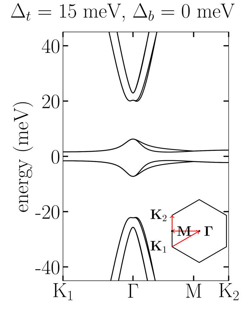
(a)

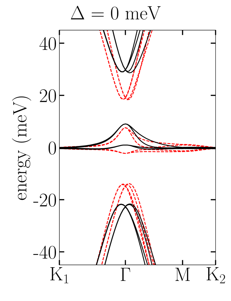
(b)

Figure 1: Bandstructures of TBG at the magic angle $\theta=1.05^{\circ}$ around charge neutrality. (a) Continuum model (CM) with out-of-plane corrugation and a substrate induced sublattice splitting of $\Delta_{t}=$15\text{\,}\frac{\mathrm{meV}}{}$$ and $\Delta_{b}=$0\text{\,}\frac{\mathrm{meV}}{}$$. (b) Tight-binding model (TBM) with in-plane lattice relaxation for two parameter systems. The black curves stands to the updated relaxation parametersNam and Koshino (2020) and the red dashed curves are taken from Ref. Nam and Koshino (2017) where the lattice relaxation was underestimated by a factor 0.42 relative to the actual lattice relaxation.

III.3 Bandgap versus Bandwidth

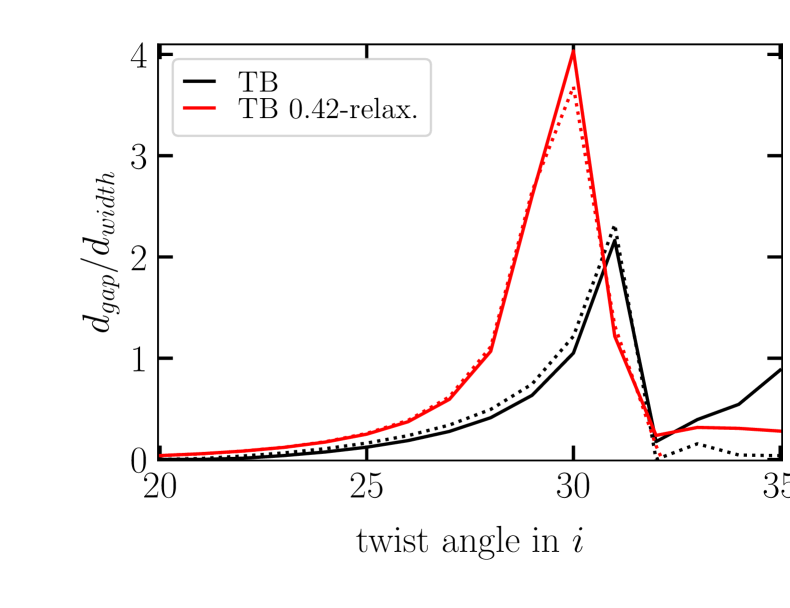
(a)

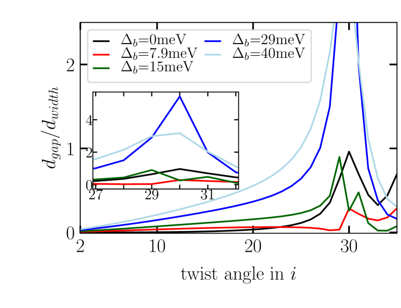
(b)

Figure 2: (a) Ratio of the gap between the flat and remote bands vs. the bandwidth of the flat bands. The solid (dashed) lines refer to the gap with respect to the upper (lower) remote bands. (b) Ratio of the gap per bandwidth, now referring to the gap between the lowest conduction and highest valence band compared to the respective conduction bandwidth. The gap at the Dirac cone was induced by the sublattice potential $\Delta_{t}=$15\text{\,}\frac{\mathrm{meV}}{}$$.

Crucial for the application of the Mielke-Tasaki theorem is the flat-band condition which is only approximate in the case of TBG. In the following, we will, therefore, assess this condition quantitatively.

The bands around charge neutrality can be regarded as nearly flat and separated from the rest of the spectrum, if the ratio of the bandgap to bandwidth $\frac{d_{gap}}{d_{width}}$ is large. This ratio is discussed in the following as function of the commensurate twist angle parametrized by the integer $i$. In this notation, the magic angle $\theta=1.05^{\circ}$ corresponds to $i=31$.

In Fig. 2(a), the bandgap between the flat bands and the remote bands is shown as it turns out for the TBM. The sublattice bias $\Delta$ is set to zero in both cases. The curves of the TBM show a maximum around the magic angle supporting the claim that the bands flatten, decreasing the bandwidth and the relative width of the gap increases.

In Fig. 2(b), we discuss the ratio in the CM focusing on the additional gap that opens up in the presence of various sublattice biases. In all cases, the splitting opens up a gap between the two valence (lower) and two conduction (upper) flat bands at the Dirac point. Again, we observe a maximum around the magic angle. Interestingly, for fixed $\Delta_{t}=15meV$, there is an optical sublattice $\Delta_{b}\sim 30$meV where the flat-band theorem can be applied.

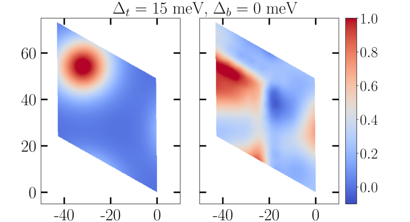
(a)

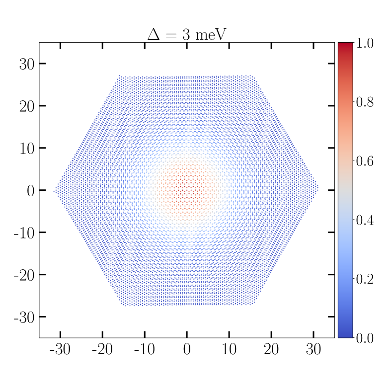
(b)

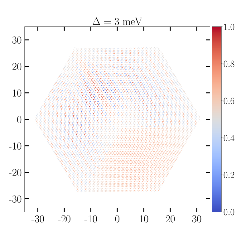
(c)

Figure 3: (a) Diagonal and off-diagonal component of the density matrix, $\rho_{ii}$ and $\rho_{i(i+m)}$ with $m=35$, as obtained from the continuum model (CM) with the parameters of Fig. 1. (b) Diagonal and (c) off-diagonal component with $m=35$ of the density matrix as obtained from the tight-binding calculations for a non-relaxed system with $\Delta=$3\text{\,}\frac{\mathrm{meV}}{}$$.

IV Density matrix of TBG

We will now discuss the central quantity of our approach, the single-particle density matrix of the four and two bands around the neutrality point, respectively.

IV.1 Density matrix of the CM

Within the CM, we solve the eigenvalue problem on an evenly spaced grid over the extended Brillouin zone, including both valleys. The density matrix $\rho_{ij}$ is then obtain from the following definition:

$$\rho_{ij} =\frac{1}{A}\sum_{n}\sum_{\mathbf{k}\in 1.BZ}e^{i\,\mathbf{k}\cdot\left(\mathbf{R}_{i}-\mathbf{R}_{j}\right)}$$ (1)

$$\times\sum_{\mathbf{G}_{1}\mathbf{G}_{2}}e^{i\,\left(\mathbf{G}_{1}\cdot\mathbf{R}_{i}-\mathbf{G}_{2}\cdot\mathbf{R}_{j}\right)}\bm{\Psi}^{\dagger}_{\mathbf{k+G}_{1},n}\bm{\Psi}_{\mathbf{k+G}_{2},n}$$

where the normalization constant is given by $A=N_{\mathbf{k}}N_{\mathbf{G}}^{2}$ and $N_{\mathbf{k}}$ denotes the number of $\mathbf{k}$-points, whereas $N_{\mathbf{G}}$ is the number of reciprocal vectors included in the calculation. $\mathbf{R}_{i}$ and $\mathbf{R}_{j}$ are the real space lattice points considered and the $n$th-eigenstate at $\mathbf{k+G}$ is denoted by $\bm{\Psi}_{\mathbf{k+G},n}$. The sum over $n$ runs either over the 4 states around the neutrality point or the 2 highest valence/2 lowest conduction band states, respectively.

The density matrix is defined on a coarsed grained unit cell and usually $\sim 100$ points are sufficient to resolve the main features. In Fig. 3(a), we display the diagonal elements $\rho_{ii}$ on the rhombic unit cell as well as an off-diagonal element $\rho_{i(i+m)}$ with $m=35$. The diagonal elements are characterized by a clear maximum at the AA-stacked region which is smeared out in the off-diagonal elements.

IV.2 Density matrix of the tight-binding model

We also calculate the density matrix with respect to the tight-binding model. In this case, $\rho_{ij}$ is given by the following formula:

$$\rho_{ij}=\frac{1}{N_{\mathbf{k}}}\sum_{n}\sum_{{\mathbf{k}}\in 1.BZ}\bm{\Psi}^{\dagger}_{\mathbf{k},n}(\mathbf{R}_{i})\bm{\Psi}_{\mathbf{k},n}(\mathbf{R}_{j})\;,$$ (2)

where $N_{\mathbf{k}}$ denotes the number of $\mathbf{k}$-points included in the calculation and $\bm{\Psi}_{\mathbf{k},n}(\mathbf{R}_{i})$ is the component at $\mathbf{R}_{i}$ of the $n$th-eigenstate at $\mathbf{k}$.

In Fig. 3(b), the diagonal elements of the density matrix for a non-relaxed system with $\Delta=$3\text{\,}\frac{\mathrm{meV}}{}$$ is plotted. In the case of the tight-binding model, the unit cell shall be resolved by the atomistic lattice sites, i.e., for $i=31$, the unit cell contains 11908 atoms and the density matrix thus has dimensions of $11908\times 11908$. Also for this model, the diagonal components show a clear maximum at the AA-stacked regions. In Fig. 3(c), we show the off-diagonal element $\rho_{i(i+m)}$ for $m=35$. Again, the diagonal matrix elements are characterized by a clear maximum at the AA-stacked region which is smeared out in the off-diagonal elements.

V Irreducibility

For both models, we have calculated the density matrix according to Eqs. (1) and (2), respectively. In order to show flat-band ferromagnetism following Mielke’s theorem, we need to show that those matrices are irreducible. An irreducible matrix is often defined by the matrix not being reducible. Since we deal only with Hermitian matrices, a sufficient condition for a matrix to be reducible is that there exists a permutation of columns and rows that transform the matrix into a block-diagonal form $\left(\begin{smallmatrix}\mathbf{A}_{11}&\mathbf{0}\\ \mathbf{0}&\mathbf{A}_{22}\end{smallmatrix}\right)$. Instead of proving the non-existence of such a permutation we employ the equivalent, but more direct, definition from graph theory: A matrix $\rho\in\mathbb{R}^{(n,n)}$, $\rho\neq 0$ is irreducible if and only if the corresponding adjacency graph is connected which shall be discussed below.

The numerical implementation of the test for irreducibility consists of two steps. First, $\rho$ is transformed into its adjacency matrix $\widehat{\rho}$, then the code tests whether $\widehat{\rho}$’s graph is connected. For our purposes, the transformation from $\rho$ into $\widehat{\rho}$ slightly differs from the usual textbook (e.g. Ref.Knaber and Barth, 2018)definition (where it would read ”$1,\,\text{ if }\rho_{ij}\neq 0$”):

$$\widehat{\rho}_{ij}\coloneqq\begin{cases}1,&\text{ if }\rho_{ij}\geq\tau\\ 0,&\text{otherwise}\end{cases}$$ (3)

where the threshold $\tau$ is a variable and can be set. By choosing $\tau$ finite, we can probe how stable the graph is connected, but we can also compensate for numerical errors that do not allow to simply set $\tau=0$. If, with a threshold higher than the numerical error, $\widehat{\rho}$ is still irreducible, one can assume that $\rho_{ij}$ itself is irreducible. In the following, we will determined a ”critical” threshold $\tau_{c}$ which we define as the largest $\tau$ that can be set before $\widehat{\rho}$ becomes reducible.

The second step in proving the graph’s connectedness is done by a path finding algorithm. The graph is connected if from every node $v_{i}$ $i\in\{1,\ldots,N\}$ every other node can be reached. Going to the assigned adjacency matrix conserves this symmetry. Density matrices are symmetric and thus is $\widehat{\rho}$. In the graph of a symmetric matrix, every connection would exist in both directions. Therefore, the algorithm only needs to find paths between nodes in one direction $v_{i}\rightarrow v_{j}$ and it immediately follows $v_{j}\rightarrow v_{i}$. Also, from $v_{j}\rightarrow v_{i}$ follows $v_{j}\rightarrow v_{k}$ $\forall k\in\{1,\ldots,N\}$ if there exists a path $v_{i}\rightarrow v_{k}$. Thus, the graph being connected is equivalent to $\exists(v_{1}\rightarrow v_{k})$ $\forall k\in\{1,\ldots,N\}$.

For the code implementation, the problem is further reduced to the question whether there exists an edge $(v_{1},v_{k})$ or alternatively an edge $(v_{k},v_{j})$ with $v_{1}\rightarrow v_{j}$. This can be treated recursively. The algorithm first finds all nodes $v_{i}$, $i\in I\subset\{2,\ldots,N\}$ with edges $(v_{1},v_{i})$ and adds them to the set of reachable nodes $M_{found}=\{1\}\oplus I$. In the next step, all nodes $v_{j}$ are found that have an edge $(v_{i},v_{j})$ and $j\neq 1\wedge j\notin I$. Those $j$ are included in $M_{found}$, $M_{found}=\{1\}\oplus I\oplus J$. The following step starts with $v_{j}$ and the scheme is repeated until $M_{found}=\{1,\ldots,N\}$ or until the element last added to $M_{found}$ has no edge with any node not yet in $M_{found}$. The way the algorithm works in the latter case implies $\not\exists(v_{i},v_{j})$ with $i\in M_{found}$ and $j\notin M_{found}$. Thus, the graph is not connected and $\rho_{ij}$ reducible. $M_{found}=\{1,\ldots,N\}$ means that all nodes have been reached, so the graph is fully connected and $\rho_{ij}$ irreducible.

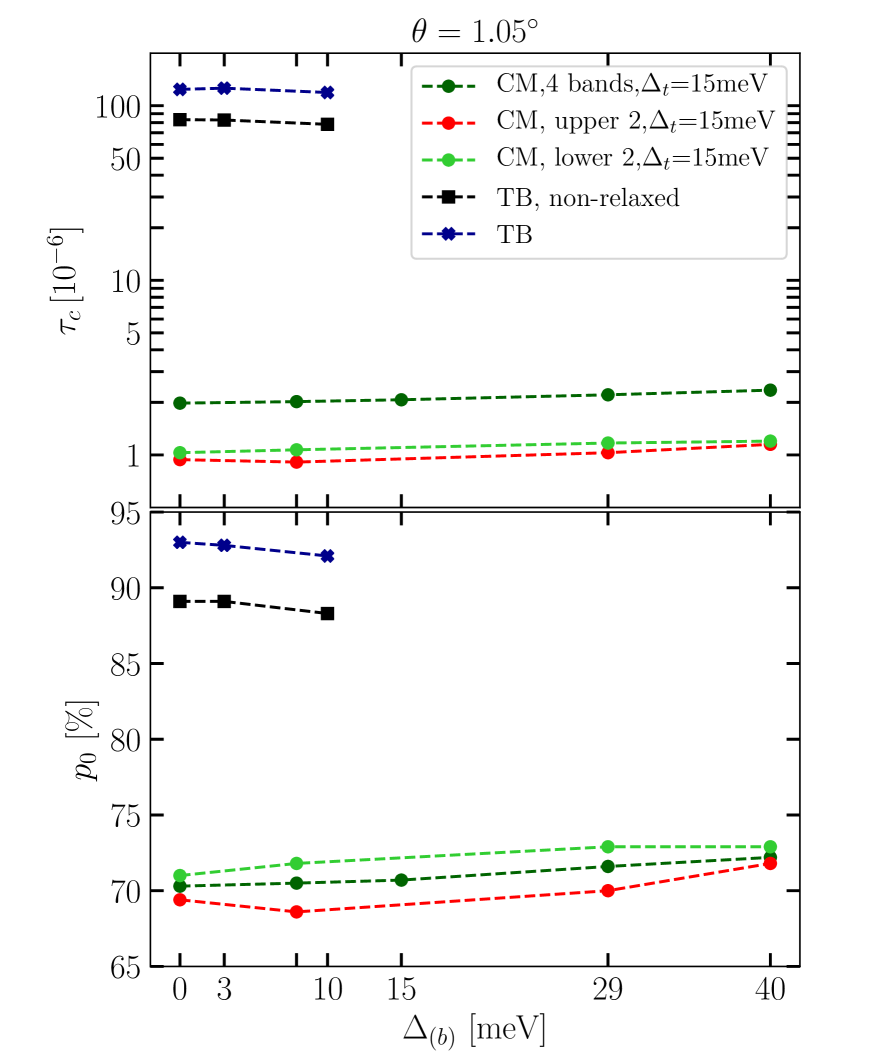
Figure 4: Thresholds $\tau_{c}$ for the density matrix at the magic angle $\theta=1.05^{\circ}$ with different models as function of the sublattice splitting $\Delta$ (TBM) or of $-\Delta_{b}$ (CM). The upper plot displays the actual value $\tau_{c}$ while the lower plot shows the percentage $p_{0}$ of the matrix elements that have been set to zero by this threshold.

VI Results

Having detailed our methods, we first present our results in form of Table 1 and 2 for the CM and the TBM, respectively. For comparison, we also analyzed the non-relaxed lattices that do not show a gap between the flat and remote bands. The column ”bands” details whether the calculation runs on all 4 flat bands or only on the conduction (upper) or valence (lower) bands. This always implies that the included flat bands are half filled: ”4” thus means ferromagnetism at charge neutrality, whereas ”lower 2” or ”upper 2” implies ferromagnetism at half-filling of the valence and conduction band, respectively.

We also considered the unrelaxed lattice and a sublattice gap $\Delta$ when we are only interested in the ground state at the neutrality point. This shows that the irreducibility of the matrix does not depend on the particular choice of parameters.

relaxed	$\Delta_{t}$ $\left[meV\right]$	$\Delta_{b}$ $\left[meV\right]$	bands	$\tau_{c}$	$p_{0}$ $\left[\%\right]$
no	0	0	4	$1.22\times 10^{-6}$	72.1
yes	0	0	4	$1.94\times 10^{-6}$	70.0
yes	15	0	4	$1.98\times 10^{-6}$	70.3
			upper 2	$9.4\times 10^{-7}$	69.4
			lower 2	$1.03\times 10^{-6}$	71.0
yes	15	-7.9	4	$2.02\times 10^{-6}$	70.5
			upper 2	$9.1\times 10^{-7}$	68.6
			lower 2	$1.07\times 10^{-6}$	71.8
yes	15	-15	4	$2.07\times 10^{-6}$	70.7
yes	15	-29	4	$2.21\times 10^{-6}$	71.6
			upper 2	$1.03\times 10^{-6}$	70.0
			lower 2	$1.17\times 10^{-6}$	72.9
yes	15	-40	4	$2.35\times 10^{-6}$	72.2
			upper 2	$1.15\times 10^{-6}$	71.8
			lower 2	$1.20\times 10^{-6}$	72.9

Table 1: Irreducibility analysis based on the density matrix obtained from the continuum model at the magic angle $\theta=1.05^{\circ}$ ($i=31$). For all parameters, the critical values are well above the numerical accuracy and the corresponding density matrix is thus irreducible.

relaxed	$\Delta$ $\left[meV\right]$	bands	$\tau_{c}$	$p_{0}$ $\left[\%\right]$
no	0	4	$8.32\times 10^{-5}$	89.1
yes	0	4	$1.24\times 10^{-4}$	93.0
no	3	4	$8.28\times 10^{-5}$	89.1
yes	3	4	$1.26\times 10^{-4}$	92.8
no	10	4	$7.82\times 10^{-5}$	88.3
yes	10	4	$1.19\times 10^{-4}$	92.1

Table 2: Irreducibility analysis based on the density matrix obtained from the tight-binding model at the magic angle $\theta=1.05^{\circ}$ ($i=31$). For all parameters, the critical values are well above the numerical accuracy and the corresponding density matrix is thus irreducible.

In Figs. 4 and 5, we present a summary of our results graphically. Additional results for the irreducibility also for other angles can be found in the Appendix B. They confirm our main conclusion that the critical values $\tau_{c}$ are much larger than the expected numerical errors. This holds, first of all, for the case where all four bands are considered and we expect ferromagnetism at half-filling. But it also holds for the case where only two bands were considered, referring to ferromagnetism at half-filling.

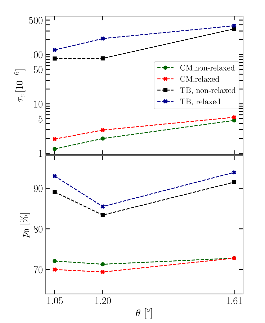
Figure 5: Thresholds $\tau_{c}$ for different angles in CM and commensurate tight-binding model without sublattice splitting.

VII Discussion and Outlook

We investigated the single particle density matrix of the almost flat bands of TBG around charge neutrality. Our main conclusion is that the single particle density matrix is irreducible for virtually all parameters. This is the main condition for flat band ferromagnetism to appear. Mielke and Tasaki (1993); Mielke (1999) Clearly, this does not prove the appearance of ferromagnetism in TBG in a mathematical sense. But we argue that nevertheless one should expect flat band ferromagnetism for the following reasons:

(i) The bands in TBG are not completely flat but there is a sufficiently large gap in the spectrum. For many other system it has been shown that flat band ferromagnetism is robust against a small dispersion of the flat band in that case and if the interaction is not too small.

(ii) In the mathematical proofs of flat band ferromagnetism the flat band needs to appear either on the bottom or on the top of the spectrum or the lattice needs to be bipartite. But one can use a perturbational argument and a conjecture on the monotonicity of $S^{2}$ as a function of $U$ to argue that flat band ferromagnetism is not restricted to these cases but can be expected in a much wider range of models and systems including TBG.

(iii) There may be further interactions present in TBG but one might expect that the Hubbard model describes the essential physics of TBG. Further, additional interactions do not necessarily disturb flat band ferromagnetism.Strack and Vollhardt (1993); Kollar and Vollhardt (2001)

Note after proof: During completion of the manuscript, we became aware of Ref. Wu and Sarma (2020) that contains a similar conclusion as ours.

VIII Acknowledgments

This work has been supported by Spain’s MINECO under Grant No. FIS2017-82260-P, by Germany’s Deutsche Forschungsgemeinschaft (DFG) via SFB 1277 as well as by the CSIC Research Platform on Quantum Technologies PTI-001.

Appendix A Hamiltonian of the continuum model

The CM’s full Hamiltonian is given by the Hamiltonian of the single unrotated layer, $H^{\mathbf{K}}_{D}$, the one of the single rotated layer, $H^{\mathbf{K}^{\theta}}_{D}$, and the interlayer coupling, $H_{T}$:

$$H_{CM}=H^{\mathbf{K}}_{D}+H^{\mathbf{K}^{\theta}}_{D}+H_{T}$$ (4)

This yields the non-zero matrix elements

$$\braket{\Psi^{(1)}_{(\mathbf{K+q}),\alpha}}{H_{CM}}{\Psi^{(2)}_{(\mathbf{K}^{\theta}+\mathbf{s}^{\theta}),\beta}}=T^{\alpha\beta}_{\mathbf{q}\mathbf{s}^{\theta}}$$ (5)

$$=T^{\alpha\beta}_{b}\delta_{\mathbf{q-s}^{\theta},\mathbf{q}_{b}}+T^{\alpha\beta}_{tr}\delta_{\mathbf{q-s}^{\theta},\mathbf{q}_{tr}}+T^{\alpha\beta}_{tl}\delta_{\mathbf{q-s}^{\theta},\mathbf{q}_{tl}}$$

the corresponding hermitian conjugates and

$$\begin{split}&\braket{\Psi^{(1)}_{(\mathbf{K+q}),\alpha}}{H_{CM}}{\Psi^{(1)}_{(\mathbf{K+s}),\beta}}\\ &=\delta_{\mathbf{q},\mathbf{s}}\left(H^{\mathbf{K}}_{D}(\mathbf{q})\right)^{\alpha\beta}\;,\end{split}$$ (6)

$$\begin{split}&\braket{\Psi^{(2)}_{(\mathbf{K}^{\theta}+\mathbf{q}^{\theta}),\alpha}}{H_{CM}}{\Psi^{(2)}_{(\mathbf{K}^{\theta}+\mathbf{s}^{\theta}),\beta}}\\ &=\delta_{\mathbf{q}^{\theta},\mathbf{s}^{\theta}}\left(H^{\mathbf{K}^{\theta}}_{D}(\mathbf{q}^{\theta})\right)^{\alpha\beta}\;,\end{split}$$ (7)

where $\left(H^{\mathbf{K}}_{D}(\mathbf{q})\right)^{\alpha\beta}$ and $\left(H^{\mathbf{K}^{\theta}}_{D}(\mathbf{q}^{\theta})\right)^{\alpha\beta}$ are elements of the matrices

$$H^{\pm\mathbf{K}}_{D}(\mathbf{q})=\pm v_{F}\left|\mathbf{q}\right|\begin{pmatrix}0&e^{\mp i\theta_{\mathbf{q}}}\\ e^{\pm i\theta_{\mathbf{q}}}&0\end{pmatrix}\;,$$ (8)

$$H^{\pm\mathbf{K}^{\theta}}_{D}(\mathbf{q})=\pm v_{F}\left|\mathbf{q}\right|\begin{pmatrix}0&e^{\mp i(\theta_{\mathbf{q}}-\theta)}\\ e^{\pm i(\theta_{\mathbf{q}}-\theta)}&0\end{pmatrix}\;.$$ (9)

The different signs stand for the different valleys and $T_{b}$, $T_{tr}$, and $T_{tl}$ areKoshino et al. (2018)

$$\begin{split}T_{b}=\begin{pmatrix}u&u^{\prime}\\ u^{\prime}&u\end{pmatrix},\qquad T_{tr}=\begin{pmatrix}ue^{i\phi}&u^{\prime}\\ u^{\prime}e^{-i\phi}&ue^{i\phi}\end{pmatrix},\\ T_{tl}=\omega\begin{pmatrix}ue^{-i\phi}&u^{\prime}\\ u^{\prime}e^{i\phi}&ue^{-i\phi}\end{pmatrix}\end{split}$$ (10)

with $\phi=\frac{2\pi}{3}$.

We will also introduce a general sublattice splitting with one bias parameter for the top layer $\Delta_{t}$ and one bias for the bottom layer $\Delta_{b}$.Bultnick19 The interlayer part of the Hamiltonian is expanded by $\Delta_{t}\sigma^{z}$ and $\Delta_{b}\sigma^{z}$, respectively, reading now

$$\braket{\Psi^{(1)}_{(\mathbf{K+q}),\alpha}}{H_{CM}}{\Psi^{(1)}_{(\mathbf{K+s}),\beta}}=\delta_{\mathbf{q},\mathbf{s}}v_{F}\left|\mathbf{q}\right|\begin{pmatrix}\Delta_{b}&e^{-i\theta_{\mathbf{q}}}\\ e^{i\theta_{\mathbf{q}}}&-\Delta_{b}\end{pmatrix}$$ (11)

$$\begin{split}&\braket{\Psi^{(2)}_{(\mathbf{K}^{\theta}+\mathbf{q}^{\theta}),\alpha}}{H_{CM}}{\Psi^{(2)}_{(\mathbf{K}^{\theta}+\mathbf{s}^{\theta}),\beta}}\\ &=\delta_{\mathbf{q}^{\theta},\mathbf{s}^{\theta}}v_{F}\left|\mathbf{q}\right|\begin{pmatrix}\Delta_{t}&e^{-i(\theta_{\mathbf{q}}-\theta)}\\ e^{i(\theta_{\mathbf{q}}-\theta)}&-\Delta_{t}\end{pmatrix}\end{split}$$ (12)

Appendix B More results on the irreducibility of the single particle density matrix

In this Appendix, we will give more details on our irreducibility analysis. In these more extensive tables, we also list numerical parameters such as the grid size $N_{\mathbf{k}}$ of the 1. Brillouin zone and the reciprocal lattice truncation $N_{\mathbf{G}}$, i.e., the number of included reciprocal lattice vectors.

For the continuum model, we also include $N_{\mathbf{R}}$ which is the number of real space points $\mathbf{R}$ used to represent the density matrix $\rho_{ij}$. $N_{bands}$ is the number of bands included where (i) ”2” means two valence bands or two conduction bands, and (ii) ”4” means two valence and two conduction bands. In both cases, the valley degree of freedom is included, whereas the spin degree of freedom is ignored.

Let us first present our results from the CM. Table 3 contains our analysis for the non-relaxed and Table 4 for the relaxed lattice of TBG, also including different sublattice biases. In both cases, 4 bands are considered predicting a ferromagnetic ground state at charge neutrality. In Table 5 and 5, we analyze the system for half-filled flat valence and conduction bands, respectively.

$\theta$ $\left[{}^{\circ}\right]$	$N_{\mathbf{G}}$	$N_{\mathbf{k}}$	$N_{\mathbf{R}}$	$N_{bands}$	$\tau$	$p_{0}$ $\left[\%\right]$
0.93	9	324	100	4	$1.29\times 10^{-6}$	77.5
1.05	9	8100	100	4	$1.09\times 10^{-6}$	71.7
1.05	9	324	100	4	$1.22\times 10^{-6}$	72.1
1.05	9	81	100	4	$1.47\times 10^{-6}$	73.2
1.12	9	324	100	4	$1.47\times 10^{-6}$	71.6
1.12	9	324	400	4	$1.47\times 10^{-6}$	69.3
1.20	9	324	100	4	$1.99\times 10^{-6}$	71.3
1.61	9	324	100	4	$4.63\times 10^{-6}$	72.8

Table 3: Threshold values for the non-relaxed TBG modeled by the CM with $u^{\prime}=u=$0.11\text{\,}\frac{\mathrm{eV}}{}$$.

$\theta$ $\left[{}^{\circ}\right]$	$\Delta_{t}$ $\left[meV\right]$	$\Delta_{b}$ $\left[meV\right]$	$N_{\mathbf{G}}$	$N_{\mathbf{k}}$	$N_{\mathbf{R}}$	$N_{bands}$	$\tau$	$p_{0}$ $\left[\%\right]$
1.61	0	0	9	324	100	4	$5.36\times 10^{-6}$	72.8
1.20	0	0	9	324	100	4	$2.95\times 10^{-6}$	69.4
1.05	0	0	9	324	100	4	$1.94\times 10^{-6}$	70.0
1.05	15	0	9	324	100	4	$1.98\times 10^{-6}$	70.3
1.05	15	-7.9	9	324	100	4	$2.02\times 10^{-6}$	70.5
1.05	15	-15	9	324	100	4	$2.07\times 10^{-6}$	70.7
1.05	15	-29	9	324	100	4	$2.21\times 10^{-6}$	71.6
1.05	15	-40	9	324	100	4	$2.35\times 10^{-6}$	72.2

Table 4: Threshold values for the relaxed lattice with $u=$0.0898\text{\,}\frac{\mathrm{eV}}{}$$, $u^{\prime}=$0.11\text{\,}\frac{\mathrm{eV}}{}$$ modeled by the CM.

$\theta$ $\left[{}^{\circ}\right]$	$\Delta_{t}$ $\left[meV\right]$	$\Delta_{b}$ $\left[meV\right]$	$N_{\mathbf{G}}$	$N_{\mathbf{k}}$	$N_{\mathbf{R}}$	$N_{bands}$	$\tau$	$p_{0}$ $\left[\%\right]$
1.05	15	0	9	324	100	2	$1.03\times 10^{-6}$	71.0
1.05	15	-7.9	9	324	100	2	$1.07\times 10^{-6}$	71.8
1.05	15	-29	9	324	100	2	$1.17\times 10^{-6}$	72.9
1.05	15	-40	9	324	100	2	$1.20\times 10^{-6}$	72.9

Table 5: Threshold values for the relaxed systems when only the lower two valence bands are considered.

$\theta$ $\left[{}^{\circ}\right]$	$\Delta_{t}$ $\left[meV\right]$	$\Delta_{b}$ $\left[meV\right]$	$N_{\mathbf{G}}$	$N_{\mathbf{k}}$	$N_{\mathbf{R}}$	$N_{bands}$	$\tau$	$p_{0}$ $\left[\%\right]$
1.05	15	0	9	324	100	2	$9.4\times 10^{-7}$	69.4
1.05	15	-7.9	9	324	100	2	$9.1\times 10^{-7}$	68.6
1.05	15	-29	9	324	100	2	$1.03\times 10^{-6}$	70.0
1.05	15	-40	9	324	100	2	$1.15\times 10^{-6}$	71.8

Table 6: Threshold values for the relaxed lattice when only the higher two conduction bands are considered.

Let us now present the detailed results coming from the tight-binding calculations, discussing different twist angles in Tabel 7. For all cases, we considered four bands around charge neutrality and chose $N_{\mathbf{k}}=900$ where convergence has been checked. In all cases, we obtain irreducibility well above the numerical error.

$\theta$ $\left[{}^{\circ}\right]$	relaxed	$\Delta$ $\left[meV\right]$	$\tau_{c}$	$p_{0}$ $\left[\%\right]$
1.05	no	0	$8.32\times 10^{-5}$	89.1
1.20	no	0	$8.37\times 10^{-5}$	83.4
1.61	no	0	$3.31\times 10^{-4}$	91.5
1.05	yes	0	$1.24\times 10^{-4}$	93.0
1.20	yes	0	$2.11\times 10^{-4}$	94.6
1.61	yes	0	$3.84\times 10^{-4}$	93.9
1.05	no	3	$8.28\times 10^{-5}$	89.1
1.05	no	10	$7.82\times 10^{-5}$	88.3
1.05	yes	3	$1.26\times 10^{-4}$	92.8
1.05	yes	10	$1.19\times 10^{-4}$	92.1

Table 7: Threshold results for the relaxed and non-relaxed lattice based on the tight-binding model.

References

- Cao et al. (2018a) Y. Cao, V. Fatemi, S. Fang, K. Watanabe, T. Taniguchi, E. Kaxiras, and P. Jarillo-Herrero, Nature 556, 43 EP (2018a).
- Yankowitz et al. (2019) M. Yankowitz, S. Chen, H. Polshyn, Y. Zhang, K. Watanabe, T. Taniguchi, D. Graf, A. F. Young, and C. R. Dean, Science 363, 1059 (2019).
- (3) S. Moriyama, Y. Morita, K. Komatsu, K. Endo, T. Iwasaki, S. Nakaharai, Y. Noguchi, Y. Wakayama, E. Watanabe, D. Tsuya, K. Watanabe, and T. Taniguchi, arXiv:1901.09356 .
- Codecido et al. (2019) E. Codecido, Q. Wang, R. Koester, S. Che, H. Tian, R. Lv, S. Tran, K. Watanabe, T. Taniguchi, F. Zhang, M. Bockrath, and C. N. Lau, Science Advances 5, eaaw9770 (2019).
- (5) C. Shen, N. Li, S. Wang, Y. Zhao, J. Tang, J. Liu, J. Tian, Y. Chu, K. Watanabe, T. Taniguchi, R. Yang, Z. Y. Meng, D. Shi, and G. Zhang, arXiv:1903.06952 .
- Lu et al. (2019) X. Lu, P. Stepanov, W. Yang, M. Xie, M. A. Aamir, I. Das, C. Urgell, K. Watanabe, T. Taniguchi, G. Zhang, A. Bachtold, A. H. MacDonald, and D. K. Efetov, Nature 574, 653 (2019).
- Chen et al. (2019) G. Chen, A. L. Sharpe, P. Gallagher, I. T. Rosen, E. J. Fox, L. Jiang, B. Lyu, H. Li, K. Watanabe, T. Taniguchi, J. Jung, Z. Shi, D. Goldhaber-Gordon, Y. Zhang, and F. Wang, Nature 572, 215 (2019).
- Xu and Balents (2018) C. Xu and L. Balents, Phys. Rev. Lett. 121, 087001 (2018).
- Volovik (2018) G. E. Volovik, JETP Letters 107, 516 (2018).
- Yuan and Fu (2018) N. F. Q. Yuan and L. Fu, Phys. Rev. B 98, 045103 (2018).
- (11) H. C. Po, L. Zou, T. Senthil, and A. Vishwanath, arXiv:1808.02482 .
- Roy and Juričić (2019) B. Roy and V. Juričić, Phys. Rev. B 99, 121407 (2019).
- Guo et al. (2018) H. Guo, X. Zhu, S. Feng, and R. T. Scalettar, Phys. Rev. B 97, 235453 (2018).
- Dodaro et al. (2018) J. F. Dodaro, S. A. Kivelson, Y. Schattner, X. Q. Sun, and C. Wang, Phys. Rev. B 98, 075154 (2018).
- (15) G. Baskaran, arXiv:1804.00627 .
- Liu et al. (2018) C.-C. Liu, L.-D. Zhang, W.-Q. Chen, and F. Yang, Phys. Rev. Lett. 121, 217001 (2018).
- Slagle and Kim (2019) K. Slagle and Y. B. Kim, SciPost Phys. 6, 16 (2019).
- Peltonen et al. (2018) T. J. Peltonen, R. Ojajärvi, and T. T. Heikkilä, Phys. Rev. B 98, 220504 (2018).
- Kennes et al. (2018) D. M. Kennes, J. Lischner, and C. Karrasch, Phys. Rev. B 98, 241407 (2018).
- Koshino et al. (2018) M. Koshino, N. F. Q. Yuan, T. Koretsune, M. Ochi, K. Kuroki, and L. Fu, Phys. Rev. X 8, 031087 (2018).
- Kang and Vafek (2018) J. Kang and O. Vafek, Phys. Rev. X 8, 031088 (2018).
- Isobe et al. (2018) H. Isobe, N. F. Q. Yuan, and L. Fu, Phys. Rev. X 8, 041041 (2018).
- You and Vishwanath (2019) Y.-Z. You and A. Vishwanath, npj Quantum Materials 4, 16 (2019).
- Wu et al. (2018) F. Wu, A. H. MacDonald, and I. Martin, Phys. Rev. Lett. 121, 257001 (2018).
- Zhang et al. (2019a) Y.-H. Zhang, D. Mao, Y. Cao, P. Jarillo-Herrero, and T. Senthil, Phys. Rev. B 99, 075127 (2019a).
- González and Stauber (2019) J. González and T. Stauber, Phys. Rev. Lett. 122, 026801 (2019).
- Ochi et al. (2018) M. Ochi, M. Koshino, and K. Kuroki, Phys. Rev. B 98, 081102 (2018).
- Thomson et al. (2018) A. Thomson, S. Chatterjee, S. Sachdev, and M. S. Scheurer, Phys. Rev. B 98, 075109 (2018).
- Carr et al. (2018) S. Carr, S. Fang, P. Jarillo-Herrero, and E. Kaxiras, Phys. Rev. B 98, 085144 (2018).
- Guinea and Walet (2018) F. Guinea and N. R. Walet, Proceedings of the National Academy of Sciences 115, 13174 (2018).
- Zou et al. (2018) L. Zou, H. C. Po, A. Vishwanath, and T. Senthil, Phys. Rev. B 98, 085435 (2018).
- González and Stauber (2020a) J. González and T. Stauber, Phys. Rev. Lett. 124, 186801 (2020a).
- González and Stauber (2020b) J. González and T. Stauber, Phys. Rev. B 102, 081118 (2020b).
- Stauber et al. (2020) T. Stauber, J. González, and G. Gómez-Santos, Phys. Rev. B 102, 081404 (2020).
- Kim et al. (2017) K. Kim, A. DaSilva, S. Huang, B. Fallahazad, S. Larentis, T. Taniguchi, K. Watanabe, B. J. LeRoy, A. H. MacDonald, and E. Tutuc, Proceedings of the National Academy of Sciences 114, 3364 (2017).
- Cao et al. (2018b) Y. Cao, V. Fatemi, A. Demir, S. Fang, S. L. Tomarken, J. Y. Luo, J. D. Sanchez-Yamagishi, K. Watanabe, T. Taniguchi, E. Kaxiras, R. C. Ashoori, and P. Jarillo-Herrero, Nature 556, 80 EP (2018b).
- Suárez Morell et al. (2010) E. Suárez Morell, J. D. Correa, P. Vargas, M. Pacheco, and Z. Barticevic, Phys. Rev. B 82, 121407 (2010).
- Bistritzer and MacDonald (2011) R. Bistritzer and A. H. MacDonald, P. Natl. Acad. Sci. Usa. 108, 12233 (2011).
- Kerelsky et al. (2019) A. Kerelsky, L. J. McGilly, D. M. Kennes, L. Xian, M. Yankowitz, S. Chen, K. Watanabe, T. Taniguchi, J. Hone, C. Dean, A. Rubio, and A. N. Pasupathy, Nature 572, 95 (2019).
- Xie et al. (2019) Y. Xie, B. Lian, B. Jäck, X. Liu, C.-L. Chiu, K. Watanabe, T. Taniguchi, B. A. Bernevig, and A. Yazdani, Nature 572, 101 (2019).
- Jiang et al. (2019) Y. Jiang, X. Lai, K. Watanabe, T. Taniguchi, K. Haule, J. Mao, and E. Y. Andrei, Nature 573, 91 (2019).
- Choi et al. (2019) Y. Choi, J. Kemmer, Y. Peng, A. Thomson, H. Arora, R. Polski, Y. Zhang, H. Ren, J. Alicea, G. Refael, F. von Oppen, K. Watanabe, T. Taniguchi, and S. Nadj-Perge, Nature Physics 15, 1174 (2019).
- Yndurain (2019) F. Yndurain, Phys. Rev. B 99, 045423 (2019).
- Lopez-Bezanilla (2019) A. Lopez-Bezanilla, Phys. Rev. Materials 3, 054003 (2019).
- Repellin et al. (2020) C. Repellin, Z. Dong, Y.-H. Zhang, and T. Senthil, Phys. Rev. Lett. 124, 187601 (2020).
- Liu et al. (2019) Y.-W. Liu, J.-B. Qiao, C. Yan, Y. Zhang, S.-Y. Li, and L. He, Phys. Rev. B 99, 201408 (2019).
- Po et al. (2018) H. C. Po, L. Zou, A. Vishwanath, and T. Senthil, Phys. Rev. X 8, 031089 (2018).
- Seo et al. (2019) K. Seo, V. N. Kotov, and B. Uchoa, Phys. Rev. Lett. 122, 246402 (2019).
- Kang and Vafek (2019) J. Kang and O. Vafek, Phys. Rev. Lett. 122, 246401 (2019).
- Zhou et al. (2007) S. Y. Zhou, G. H. Gweon, A. V. Fedorov, P. N. First, W. A. de Heer, D. H. Lee, F. Guinea, A. H. Castro Neto, and A. Lanzara, Nature Materials 6, 770 (2007).
- Hunt et al. (2013) B. Hunt, J. D. Sanchez-Yamagishi, A. F. Young, M. Yankowitz, B. J. LeRoy, K. Watanabe, T. Taniguchi, P. Moon, M. Koshino, P. Jarillo-Herrero, and R. C. Ashoori, Science 340, 1427 (2013).
- Sharpe et al. (2019) A. L. Sharpe, E. J. Fox, A. W. Barnard, J. Finney, K. Watanabe, T. Taniguchi, M. A. Kastner, and D. Goldhaber-Gordon, Science 365, 605 (2019).
- Serlin et al. (2020) M. Serlin, C. L. Tschirhart, H. Polshyn, Y. Zhang, J. Zhu, K. Watanabe, T. Taniguchi, L. Balents, and A. F. Young, Science 367, 900 (2020).
- Bultinck et al. (2020a) N. Bultinck, S. Chatterjee, and M. P. Zaletel, Phys. Rev. Lett. 124, 166601 (2020a).
- Zhang et al. (2019b) Y.-H. Zhang, D. Mao, and T. Senthil, Phys. Rev. Research 1, 033126 (2019b).
- Chatterjee et al. (2020) S. Chatterjee, N. Bultinck, and M. P. Zaletel, Phys. Rev. B 101, 165141 (2020).
- Liu and Dai (2020) J. Liu and X. Dai, npj Computational Materials 6, 57 (2020).
- Wu et al. (2019) X.-C. Wu, A. Keselman, C.-M. Jian, K. A. Pawlak, and C. Xu, Phys. Rev. B 100, 024421 (2019).
- (59) Y. Alavirad and J. D. Sau, arXiv:1907.13633 .
- Mielke and Tasaki (1993) A. Mielke and H. Tasaki, Comm. Math. Phys. 158, 341 (1993).
- Mielke (1999) A. Mielke, Journal of Physics A: Mathematical and General 32, 8411 (1999).
- Tasaki (2020) H. Tasaki, Physics and Mathematics of Quantum Many-Body Systems, Graduate Texts in Physics (Springer Nature Switzerland AG, 2020).
- Bahamon et al. (2020) D. A. Bahamon, G. Gómez-Santos, and T. Stauber, Nanoscale 12, 15383 (2020).
- Bultinck et al. (2020b) N. Bultinck, E. Khalaf, S. Liu, S. Chatterjee, A. Vishwanath, and M. P. Zaletel, Phys. Rev. X 10, 031034 (2020b).
- Assaad and Herbut (2013) F. F. Assaad and I. F. Herbut, Phys. Rev. X 3, 031010 (2013).
- Lieb (1989) E. H. Lieb, Phys. Rev. Lett. 62, 1201 (1989).
- Sütö (91ff) A. Sütö, private communication (1991ff).
- Tasaki (1994) H. Tasaki, Phys. Rev. Lett. 73, 1158 (1994).
- Tasaki (1996) H. Tasaki, J. Stat. Phys. 84, 535 (1996).
- Tanaka and Ueda (2003) A. Tanaka and H. Ueda, Phys. Rev. Lett. 90, 67204 (2003).
- Lopes dos Santos et al. (2007) J. M. B. Lopes dos Santos, N. M. R. Peres, and A. H. Castro Neto, Phys. Rev. Lett. 99, 256802 (2007).
- Mele (2010) E. J. Mele, Phys. Rev. B 81, 161405 (2010).
- Moon and Koshino (2012) P. Moon and M. Koshino, Phys. Rev. B 85, 195458 (2012).
- de Laissardière et al. (2010) G. T. de Laissardière, D. Mayou, and L. Magaud, Nano Letters 10, 804 (2010).
- Kim et al. (2018) H. Kim, N. Leconte, B. L. Chittari, K. Watanabe, T. Taniguchi, A. H. MacDonald, J. Jung, and S. Jung, Nano Letters 18, 7732 (2018).
- Brihuega et al. (2012) I. Brihuega, P. Mallet, H. González-Herrero, G. Trambly de Laissardière, M. M. Ugeda, L. Magaud, J. M. Gómez-Rodríguez, F. Ynduráin, and J.-Y. Veuillen, Phys. Rev. Lett. 109, 196802 (2012).
- Moon and Koshino (2013) P. Moon and M. Koshino, Phys. Rev. B 87, 205404 (2013).
- Nam and Koshino (2017) N. N. T. Nam and M. Koshino, Phys. Rev. B 96, 075311 (2017).
- Nam and Koshino (2020) N. N. T. Nam and M. Koshino, Phys. Rev. B 101, 099901 (2020).
- Knaber and Barth (2018) P. Knaber and W. Barth, Lineare Arlgebra (Grundlagen und Anwendungen), 2nd ed. (Springer Spektrum, Berlin, Heidelberg, 2018).
- Strack and Vollhardt (1993) R. Strack and D. Vollhardt, Phys. Rev. Lett. 70, 2637 (1993).
- Kollar and Vollhardt (2001) M. Kollar and D. Vollhardt, Phys. Rev. B 63, 045107 (2001).
- Wu and Sarma (2020) F. Wu and S. D. Sarma, “Quantum geometry and stability of moiré flatband ferromagnetism,” (2020), arXiv:2005.10254 [cond-mat.str-el] .