Auto-Sklearn 2.0: Hands-free AutoML via Meta-Learning

Abstract

Automated Machine Learning (AutoML) supports practitioners and researchers with the tedious task of designing machine learning pipelines and has recently achieved substantial success. In this paper, we introduce new AutoML approaches motivated by our winning submission to the second ChaLearn AutoML challenge. We develop PoSH Auto-sklearn, which enables AutoML systems to work well on large datasets under rigid time limits by using a new, simple and meta-feature-free meta-learning technique and by employing a successful bandit strategy for budget allocation. However, PoSH Auto-sklearn introduces even more ways of running AutoML and might make it harder for users to set it up correctly. Therefore, we also go one step further and study the design space of AutoML itself, proposing a solution towards truly hands-free AutoML. Together, these changes give rise to the next generation of our AutoML system, Auto-sklearn 2.0. We verify the improvements by these additions in an extensive experimental study on $39$ AutoML benchmark datasets. We conclude the paper by comparing to other popular AutoML frameworks and Auto-sklearn 1.0, reducing the relative error by up to a factor of $4.5$, and yielding a performance in 10 minutes that is substantially better than what Auto-sklearn 1.0 achieves within an hour.

Keywords: Automated machine learning, hyperparameter optimization, meta-learning, automated AutoML, benchmark

1 Introduction

The recent substantial progress in machine learning (ML) has led to a growing demand for hands-free ML systems that can support developers and ML novices in efficiently creating new ML applications. Since different datasets require different ML pipelines, this demand has given rise to the area of automated machine learning (AutoML; Hutter et al., 2019). Popular AutoML systems, such as Auto-WEKA (Thornton et al., 2013), hyperopt-sklearn (Komer et al., 2014), Auto-sklearn (Feurer et al., 2015a), TPOT (Olson et al., 2016a) and Auto-Keras (Jin et al., 2019) perform a combined optimization across different preprocessors, classifiers or regressors and their hyperparameter settings, thereby reducing the effort for users substantially.

To assess the current state of AutoML and, more importantly, to foster progress in AutoML, ChaLearn conducted a series of AutoML challenges (Guyon et al., 2019), which evaluated AutoML systems in a systematic way under rigid time and memory constraints. Concretely, in these challenges, the AutoML systems were required to deliver predictions in less than $20$ minutes. On the one hand, this would allow to efficiently integrate AutoML into the rapid prototype-driven workflow of many data scientists and, on the other hand, help to democratize ML by requiring less compute resources.

We won both the first and second AutoML challenge with modified versions of Auto-sklearn. In this work, we describe in detail how we improved Auto-sklearn from the first version (Feurer et al., 2015a) to construct PoSH Auto-sklearn, which won the second competition and then describe how we improved PoSH Auto-sklearn further to yield our current approach for Auto-sklearn 2.0.

Particularly, while AutoML relieves the user from making low-level design decisions (e.g. which model to use), AutoML itself opens a myriad of high-level design decisions, e.g. which model selection strategy to use (Guyon et al., 2010, 2015; Raschka, 2018) or how to allocate the given time budget (Jamieson and Talwalkar, 2016). Whereas our submissions to the AutoML challenges were mostly hand-designed, in this work, we go one step further by automating AutoML itself to fully unfold the potential of AutoML in practice.

After detailing the AutoML problem we consider in Section 2, we present two main parts making the following contributions:

Part I: Portfolio Successive Halving in PoSH Auto-sklearn.

In this part (see Section 3), we introduce budget allocation strategies as a complementary design choice to model selection strategies (holdout (HO) and cross-validation (CV)) for AutoML systems. We suggest using the budget allocation strategy successive halving (SH) as an alternative to always using the full budget (FB) to evaluate a configuration to allocate more resources to promising ML pipelines. Furthermore, we introduce both the practical approach as well as the theory behind building better portfolios for the meta-learning component of Auto-sklearn. We show that this combination substantially improves performance, yielding stronger results in 10 minutes than Auto-sklearn 1.0 achieved in 60 minutes.

Part II: Automating AutoML in Auto-sklearn 2.0.

In this part (see Section 4), we propose a meta-learning technique based on algorithm selection to automatically select the best setting of the AutoML system itself for a given dataset. We dub the resulting system Auto-sklearn 2.0 and depict the evolution from Auto-sklearn 1.0 via PoSH Auto-sklearn to Auto-sklearn 2.0 in Figure 1.

In Section 5, we additionally use the AutoML benchmark (Gijsbers et al., 2019) to evaluate Auto-sklearn 2.0 against other popular AutoML systems and show improved performance under rigid time constraints. Section 6 then puts our work into the context of related works, and Section 7 concludes the paper with open questions, limitations and future work.

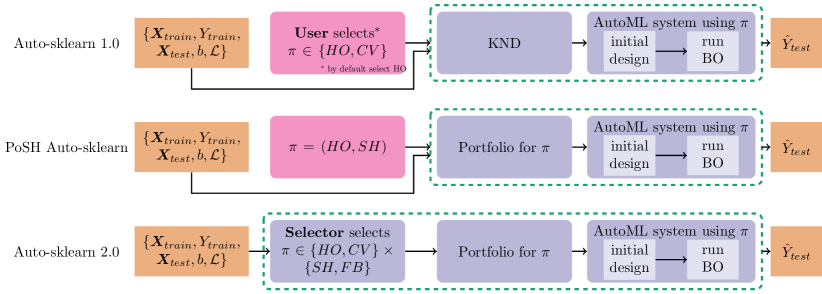
Figure 1: Schematic overview of Auto-sklearn 1.0, PoSH Auto-sklearn, and Auto-sklearn 2.0. Orange rectangular boxes refer to input and output data, while rounded purple boxes denote parts of the AutoML system (surrounded by a green dashed line). The pink, rounded box refers to a human in the loop required for manual design decisions. The newer AutoML systems simplify the usage of Auto-sklearn and reduce the required user input. We describe PoSH Auto-sklearn in Section 3 and give a schematic overview in Figure 2. Similarly, we describe Auto-sklearn 2.0 in Section 4 and provide a schematic overview in Figure 5.

2 Problem Statement

AutoML is a widely used term, so, here we first define the problem we consider in this work. Let $P(\mathcal{D})$ be a distribution of datasets from which we can sample an individual dataset’s distribution $P_{d}=P_{d}(\mathbf{x},y)$. The AutoML problem we consider is to generate a trained pipeline $\mathcal{M}_{{\bm{\lambda}}}:\mathbf{x}\mapsto y$, hyperparameterized by ${\bm{\lambda}}\in{\bm{\Lambda}}$ that automatically produces predictions for samples from the distribution $P_{d}$ minimizing the expected generalization error:

$$GE(\mathcal{M}_{\bm{\lambda}})=\mathds{E}_{(\mathbf{x},y)\sim P_{d}}\left[\mathcal{L}(\mathcal{M}_{\bm{\lambda}}(\mathbf{x}),y)\right].$$ (1)

Since a dataset can only be observed through a set of $n$ independent observations $\mathcal{D}_{d}=\{(\mathbf{x}_{1},y_{1}),\dots,(\mathbf{x}_{n},y_{n})\}\sim P_{d}$, we can only empirically approximate the generalization error on sample data:

$$\savestack{\tmpbox}{\stretchto{\scaleto{\scalerel*[\widthof{GE}]{\kern-0.6pt\bigwedge\kern-0.6pt}{\rule[-614.295pt]{4.30554pt}{614.295pt}}}{}}{0.5ex}}\stackon[1pt]{GE}{\tmpbox}(\mathcal{M}_{\bm{\lambda}},\mathcal{D}_{d})=\frac{1}{n}\sum_{i=1}^{n}\mathcal{L}(\mathcal{M}_{\bm{\lambda}}(\mathbf{x}_{i}),y_{i}).$$ (2)

In practice we have access to two disjoint, finite samples which we from now on denote $\mathcal{D}_{\text{train}}$ and $\mathcal{D}_{\text{test}}$ ($\mathcal{D}_{d,\text{train}}$ and $\mathcal{D}_{d,\text{test}}$ in case we reference a specific dataset $P_{d}$). For searching the best ML pipeline, we only have access to $\mathcal{D}_{\text{train}}$, however, in the end performance is estimated once on $\mathcal{D}_{\text{test}}$. AutoML systems use this to automatically search for the best $\mathcal{M}_{{\bm{\lambda}}^{*}}$:

$$\mathcal{M}_{{\bm{\lambda}}^{*}}\in\operatorname*{argmin}_{{\bm{\lambda}}\in{\bm{\Lambda}}}\savestack{\tmpbox}{\stretchto{\scaleto{\scalerel*[\widthof{GE}]{\kern-0.6pt\bigwedge\kern-0.6pt}{\rule[-614.295pt]{4.30554pt}{614.295pt}}}{}}{0.5ex}}\stackon[1pt]{GE}{\tmpbox}(\mathcal{M}_{\bm{\lambda}},\mathcal{D}_{\text{train}}),$$ (3)

and estimate GE, e.g., by a $K$-fold cross-validation:

$$\savestack{\tmpbox}{\stretchto{\scaleto{\scalerel*[\widthof{GE}]{\kern-0.6pt\bigwedge\kern-0.6pt}{\rule[-614.295pt]{4.30554pt}{614.295pt}}}{}}{0.5ex}}\stackon[1pt]{GE}{\tmpbox}_{\text{CV}}(\mathcal{M}_{\bm{\lambda}},\mathcal{D}_{\text{train}})=\frac{1}{K}\sum_{k=1}^{K}\savestack{\tmpbox}{\stretchto{\scaleto{\scalerel*[\widthof{GE}]{\kern-0.6pt\bigwedge\kern-0.6pt}{\rule[-614.295pt]{4.30554pt}{614.295pt}}}{}}{0.5ex}}\stackon[1pt]{GE}{\tmpbox}(\mathcal{M}_{\bm{\lambda}}^{\mathcal{D}_{\text{train}}^{(\text{train},k)}},{\mathcal{D}_{\text{train}}^{(\text{val},k)}}),$$ (4)

where $\mathcal{M}_{\bm{\lambda}}^{\mathcal{D}_{\text{train}}^{(\text{train},k)}}$ denotes that $\mathcal{M}_{\bm{\lambda}}$ was trained on the training split of $k$-th fold $\mathcal{D}_{\text{train}}^{(\text{train},k)}\subset\mathcal{D}_{\text{train}}$, and it is then evaluated on the validation split of the $k$-th fold $\mathcal{D}_{\text{train}}^{(\text{val},k)}=\mathcal{D}_{\text{train}}\setminus\mathcal{D}_{\text{train}}^{(\text{train},k)}$. Assuming that, via ${\bm{\lambda}}$, an AutoML system can select both, an algorithm and its hyperparameter settings, this definition using $\savestack{\tmpbox}{\stretchto{\scaleto{\scalerel*[\widthof{GE}]{\kern-0.6pt\bigwedge\kern-0.6pt}{\rule[-614.295pt]{4.30554pt}{614.295pt}}}{}}{0.5ex}}\stackon[1pt]{GE}{\tmpbox}_{\text{CV}}$ is equivalent to the definition of the CASH (Combined Algorithm Selection and Hyperparameter optimization) problem (Thornton et al., 2013; Feurer et al., 2015a). However, it is unlikely that, whatever optimization algorithm we use, the AutoML system finds the exact optimum location ${\bm{\lambda}}^{*}$. Instead, the AutoML system will return the best ML pipeline it has trained during the search process, which we denote by $\mathcal{M}_{\hat{{\bm{\lambda}}}^{*}}$, and the hyperparameter settings it was trained with by $\hat{{\bm{\lambda}}}^{*}$.

2.1 Time-bounded AutoML

In practice, users are not only interested in obtaining an optimal pipeline $\mathcal{M}_{{\bm{\lambda}}^{*}}$ eventually, but have constraints on how much time and compute resources they are willing to invest. We denote the time it takes to evaluate $\savestack{\tmpbox}{\stretchto{\scaleto{\scalerel*[\widthof{GE}]{\kern-0.6pt\bigwedge\kern-0.6pt}{\rule[-614.295pt]{4.30554pt}{614.295pt}}}{}}{0.5ex}}\stackon[1pt]{GE}{\tmpbox}(\mathcal{M}_{{\bm{\lambda}}},\mathcal{D}_{\text{train}})$ as $t_{{\bm{\lambda}}}$ and the overall optimization budget by $T$. Our goal is to find

$$\mathcal{M}_{{\bm{\lambda}}^{*}}\in\operatorname*{argmin}_{{\bm{\lambda}}\in{\bm{\Lambda}}}\savestack{\tmpbox}{\stretchto{\scaleto{\scalerel*[\widthof{GE}]{\kern-0.6pt\bigwedge\kern-0.6pt}{\rule[-614.295pt]{4.30554pt}{614.295pt}}}{}}{0.5ex}}\stackon[1pt]{GE}{\tmpbox}(\mathcal{M}_{\bm{\lambda}},\mathcal{D}_{\text{train}})\text{ s.t.}\left(\sum t_{{\bm{\lambda}}_{i}}\right)<T$$ (5)

where the sum is over all evaluated pipelines ${\bm{\lambda}}_{i}$, explicitly honouring the optimization budget $T$. As before, the AutoML system will return the best model it has found within the optimization budget, $\mathcal{M}_{\hat{{\bm{\lambda}}}^{*}}$.

2.2 Generalization of AutoML

Ultimately, an AutoML system $\mathcal{A}:\mathcal{D}\mapsto\mathcal{M}_{\hat{{\bm{\lambda}}}^{*}}^{\mathcal{D}}$ should not only perform well on a single dataset but on the entire distribution over datasets $P(\mathcal{D})$. Therefore, the meta-problem of AutoML can be formalized as minimizing the generalization error over this distribution of datasets:

$$GE(\mathcal{A})=\mathds{E}_{\mathcal{D}_{d}\sim P(\mathcal{D})}\left[\savestack{\tmpbox}{\stretchto{\scaleto{\scalerel*[\widthof{GE}]{\kern-0.6pt\bigwedge\kern-0.6pt}{\rule[-614.295pt]{4.30554pt}{614.295pt}}}{}}{0.5ex}}\stackon[1pt]{GE}{\tmpbox}(\mathcal{A}(\mathcal{D}_{d}),\mathcal{D}_{d})\right],$$ (6)

which in turn can again only be approximated by a finite set of meta-train datasets $\mathbf{D}_{\text{meta}}$ (each with a finite set of observations):

$$\savestack{\tmpbox}{\stretchto{\scaleto{\scalerel*[\widthof{GE}]{\kern-0.6pt\bigwedge\kern-0.6pt}{\rule[-614.295pt]{4.30554pt}{614.295pt}}}{}}{0.5ex}}\stackon[1pt]{GE}{\tmpbox}(\mathcal{A},\mathbf{D}_{\text{meta}})=\frac{1}{\mid\mathbf{D}_{\text{meta}}\mid}\sum_{d=1}^{|\mathbf{D}_{\text{meta}}|}\savestack{\tmpbox}{\stretchto{\scaleto{\scalerel*[\widthof{GE}]{\kern-0.6pt\bigwedge\kern-0.6pt}{\rule[-614.295pt]{4.30554pt}{614.295pt}}}{}}{0.5ex}}\stackon[1pt]{GE}{\tmpbox}(\mathcal{A}(\mathcal{D}_{d}),\mathcal{D}_{d}).$$ (7)

Having set up the problem statement, we can use this to further formalize our goals. Instead of using a single, fixed AutoML system $\mathcal{A}$, we will introduce optimization policies $\pi$, a combination of hyperparameters of the AutoML system and specific components to be used in a run, which can be used to configure an AutoML system for specific use cases. We then denote such a configured AutoML system as $\mathcal{A}_{\pi}$.

We will first construct $\pi$ manually in Section 3, introduce a novel system for designing $\pi$ from data in Section 4 and then extend this to a (learned) mapping $\Xi:\mathcal{D}\rightarrow\pi$ which automatically suggests an optimization policy for a new dataset using algorithm selection. This problem setup can also be used to introduce generalizations of the algorithm selection problem such as algorithm configuration (Birattari et al., 2002; Hutter et al., 2009; Kleinberg et al., 2017), per-instance algorithm configuration (Xu et al., 2010; Malitsky et al., 2012) and dynamic algorithm configuration (Biedenkapp et al., 2020) on a meta-level; but we leave these for future work. In addition, instead of selecting between multiple policies of a single AutoML system, the presented method can be applied to choose between different AutoML systems without adjustments. However, instead of maximizing performance by invoking many AutoML systems, thereby increasing the complexity, our goal is to improve single AutoML systems to make them easier to use by decreasing complexity for the user.

3 Part I: Portfolio Successive Halving in PoSH Auto-sklearn

In this section we introduce our winning solution for the second AutoML competition (Guyon et al., 2019), PoSH Auto-sklearn, short for Portfolio Successive Halving. We first describe our use of portfolios to warmstart an AutoML system and then motivate using the successive halving bandit strategy. Next, we describe practical considerations for building PoSH Auto-sklearn, give a schematic overview and recap additional handcrafted techniques we used in the competition. We end this first part of our main contributions with an experimental evaluation demonstrating the performance of PoSH Auto-sklearn.

3.1 Portfolio Building

Finding the optimal solution to the time-bounded optimization problem from Equation (5) requires searching a large space of possible ML pipelines as efficiently as possible. BO is a strong approach for this, but its vanilla version starts from scratch for every new problem. A better solution is to warmstart BO with ML pipelines that are expected to work well, as done in the k-nearest dataset (KND) approach of Auto-sklearn 1.0 (Reif et al., 2012; Feurer et al., 2015b, a; see also the related work in Section 6.4.1). However, we found this solution to introduce new problems:

1. It is time-consuming since it requires to compute meta-features describing the characteristics of datasets.

2. It adds complexity to the system as the computation of the meta-features must also be done with a time and memory limit.

3. Many meta-features are not defined with respect to categorical features and missing values, making them hard to apply for most datasets.

4. It is not immediately clear which meta-features work best for which problem.

5. In the KND approach, there is no mechanism to guarantee that we do not execute redundant ML pipelines.

We indeed suffered from these issues in the first AutoML challenge, failing on one track due to running over time for the meta-feature generation, although we had already removed landmarking meta-features due to their potentially high runtime. Therefore, here we propose a meta-feature-free approach that does not warmstart with a set of configurations specific to a new dataset, but which uses a static portfolio – a set of complementary configurations that covers as many diverse datasets as possible and minimizes the risk of failure when facing a new task.

So, instead of evaluating configurations chosen online by the KND method, we construct a portfolio, consisting of high-performing and complementary ML pipelines to perform well on as many datasets as possible, offline. Then, for a dataset at hand, all pipelines in this portfolio are simply evaluated one after the other. If time is left afterwards, we continue with pipelines suggested by BO warmstarted with the evaluated portfolio pipelines. We introduce portfolio-based warmstarting to avoid computing meta-features for a new dataset. However, the portfolios also work inherently differently. While the KND method is aimed at using only well-performing configurations, a portfolio is built such that there is a diverse set of configurations, starting with ones that perform well on average and then moving to more specialized ones. Thus, it can be seen as an optimized initial design for the BO method.

In the following, we describe our offline procedure for constructing such a portfolio and give theoretical underpinning by a performance bound.

3.1.1 Approach

We first describe how we construct a portfolio given a finite set of candidate pipelines $\mathcal{C}=\{{\bm{\lambda}}_{1},...,{\bm{\lambda}}_{l}\}$. Additionally, we assume that there exists a set of datasets $\mathbf{D}_{\text{meta}}=\{\mathcal{D}_{1},\dots,\mathcal{D}_{|\mathbf{D}_{\text{meta}}|}$} and we wish to build a portfolio $\mathcal{P}$ consisting of a subset of the pipelines in $\mathcal{C}$ that performs well on $\mathbf{D}_{\text{meta}}$.

We outline the process to build such a portfolio in Algorithm 1. First, we initialize our portfolio $\mathcal{P}$ to the empty set (Line 2). Then, we repeat the following procedure until $|\mathcal{P}|$ reaches a pre-defined limit: From a set of candidate ML pipelines $\mathcal{C}$, we greedily add a candidate ${\bm{\lambda}}^{+}\in\mathcal{C}$ to $\mathcal{P}$ that reduces the estimated generalization error over all meta-datasets most (Line 4), and then remove ${\bm{\lambda}}^{+}$ from $\mathcal{C}$ (Line 5).

The estimated generalization error of a portfolio $\mathcal{P}$ on a single dataset $\mathcal{D}$ is the performance of the best pipeline ${\bm{\lambda}}\in\mathcal{P}$ on $\mathcal{D}$ according to the model selection and budget allocation strategy. This can be described via a function $S(\cdot,\cdot,\cdot)$, which takes as input a function to compute the estimated generalization error (e.g., as defined in Equation 4), a set of machine learning pipelines to train, and a dataset. It then returns the pipeline with the lowest estimated generalization error as

$$\mathcal{M}_{{\bm{\lambda}}^{*}}^{\mathcal{D}}=S(\savestack{\tmpbox}{\stretchto{\scaleto{\scalerel*[\widthof{GE}]{\kern-0.6pt\bigwedge\kern-0.6pt}{\rule[-614.295pt]{4.30554pt}{614.295pt}}}{}}{0.5ex}}\stackon[1pt]{GE}{\tmpbox},\mathcal{P},\mathcal{D})\in\operatorname*{argmin}_{\mathcal{M}_{{\bm{\lambda}}}^{\mathcal{D}}\in\mathcal{P}}\savestack{\tmpbox}{\stretchto{\scaleto{\scalerel*[\widthof{GE}]{\kern-0.6pt\bigwedge\kern-0.6pt}{\rule[-614.295pt]{4.30554pt}{614.295pt}}}{}}{0.5ex}}\stackon[1pt]{GE}{\tmpbox}(\mathcal{M}_{{\bm{\lambda}}}^{\mathcal{D}},\mathcal{D}).$$ (8)

In case the result of $\operatorname*{argmin}$ is not unique, we return the model that was evaluated first. The estimated generalization error of $\mathcal{P}$ across all meta-datasets $\mathbf{D}_{\text{meta}}=\{\mathcal{D}_{1},\dots,\mathcal{D}_{|\mathbf{D}_{\text{meta}}|}\}$ is then

$$\savestack{\tmpbox}{\stretchto{\scaleto{\scalerel*[\widthof{GE}]{\kern-0.6pt\bigwedge\kern-0.6pt}{\rule[-614.295pt]{4.30554pt}{614.295pt}}}{}}{0.5ex}}\stackon[1pt]{GE}{\tmpbox}_{S}(\mathcal{P},\mathbf{D}_{\text{meta}})=\sum_{d=1}^{|\mathbf{D}_{\text{meta}}|}\savestack{\tmpbox}{\stretchto{\scaleto{\scalerel*[\widthof{GE}]{\kern-0.6pt\bigwedge\kern-0.6pt}{\rule[-614.295pt]{4.30554pt}{614.295pt}}}{}}{0.5ex}}\stackon[1pt]{GE}{\tmpbox}\left(S\left(\savestack{\tmpbox}{\stretchto{\scaleto{\scalerel*[\widthof{GE}]{\kern-0.6pt\bigwedge\kern-0.6pt}{\rule[-614.295pt]{4.30554pt}{614.295pt}}}{}}{0.5ex}}\stackon[1pt]{GE}{\tmpbox},\mathcal{P},\mathcal{D}_{d}\right),\mathcal{D}_{d}^{\text{val}}\right),$$ (9)

Here, we give the equation for using holdout, and in Appendix A we provide the exact notation for cross-validation and successive halving.

1:  Input: Set of candidate ML pipelines $\mathcal{C}$, $\mathbf{D}_{\text{meta}}=\{\mathcal{D}_{1},\dots,\mathcal{D}_{|\mathbf{D}_{\text{meta}}|}\}$, maximal portfolio size $p$, model selection strategy $S$ 2:  $\mathcal{P}=\emptyset$ 3:  while $|\mathcal{P}|<p$ do 4:     ${\bm{\lambda}}^{+}=\operatorname*{argmin}_{{\bm{\lambda}}\in\mathcal{C}}\savestack{\tmpbox}{\stretchto{\scaleto{\scalerel*[\widthof{GE}]{\kern-0.6pt\bigwedge\kern-0.6pt}{\rule[-614.295pt]{3.87498pt}{614.295pt}}}{}}{0.5ex}}\stackon[1pt]{GE}{\tmpbox}_{S}(\mathcal{P}\cup\{{\bm{\lambda}}\},\mathbf{D}_{\text{meta}})$ // Ties are broken favoring the model trained first. 5:     $\mathcal{P}=\mathcal{P}\cup{\bm{\lambda}}^{+},\text{ }\mathcal{C}=\mathcal{C}\setminus\{{\bm{\lambda}}^{+}\}$ 6:  end while 7:  return  Portfolio $\mathcal{P}$

Algorithm 1 Greedy Portfolio Building

We now detail how to construct the set of candidate pipelines $\mathcal{C}$ and describe how finding the candidate pipelines and constructing the portfolio fit in the larger picture. We give a schematic overview of this process in Figure 2. It consists of a training (TR1–TR3) and a testing stage (TE1–TE2).

Having collected datasets $\mathbf{D}_{\text{meta}}$ (we describe in Section 3.4.1 how we did this for our experiments), we obtain the candidate ML pipelines (TR1) by running Auto-sklearn without meta-learning and without ensembling on each dataset. We limit ourselves to a finite set of portfolio candidates $\mathcal{C}$, and pick one candidate per dataset. Then, we build a performance matrix of size $|\mathcal{C}|\times|\mathbf{D}_{\text{meta}}|$ by evaluating each of these candidate pipelines on each dataset (TR2, we refer to Section 3.4.2 for a detailed description of the meta-data generation). Finally, we then use this matrix to build a portfolio using Algorithm 1 for the combination of model selection strategy holdout and budget allocation strategy SH in training step TR3.

For a new dataset $\mathcal{D}_{\text{new}}\in\mathbf{D}_{\text{test}}{}$, we apply the AutoML system using SH, holdout and the portfolio to $\mathcal{D}_{\text{new}}$ (TE1). Finally, we return the best found pipeline $\mathcal{M}_{\hat{{\bm{\lambda}}}^{*}}$, or an ensemble of the evaluated pipelines, based on the training set of $\mathcal{D}_{\text{new}}$ (TE2.1). Optionally, we can then compute the loss of $\mathcal{M}_{\hat{{\bm{\lambda}}}^{*}}$ on the test set of $\mathcal{D}_{\text{new}}$ (TE2.2); we emphasize that this would be the only time we ever access the test set of $\mathcal{D}_{\text{new}}$.

To build a portfolio across datasets, we need to take into account that the generalization errors for different datasets live on different scales (Bardenet et al., 2013). Thus, before taking averages, for each dataset, we transform the generalization errors to the distance to the best observed performance scaled between zero and one, a metric named distance to minimum; which when averaged across all datasets is known as average distance to the minimum (ADTM) (Wistuba et al., 2015a, 2018). We compute the statistics for zero-one scaling individually for each combination of model selection and budget allocation (i.e., we use the lowest observed test loss and the largest observed test loss for each meta-dataset).

For each meta-dataset $\mathcal{D}_{d}\in\mathbf{D}_{\text{meta}}$ we have access to both $\mathcal{D}_{d,\text{train}}$ and $\mathcal{D}_{d,\text{test}}$. In the case of holdout, we split the training set $\mathcal{D}_{d,\text{train}}$ into two smaller disjoint sets $\mathcal{D}^{\text{train}}_{d,\text{train}}$ and $\mathcal{D}^{\text{val}}_{d,\text{train}}$. We usually train models using $\mathcal{D}^{\text{train}}_{d,\text{train}}$ and use $\mathcal{D}^{\text{val}}_{d,\text{train}}$ to choose a ML pipeline $\mathcal{M}_{{\bm{\lambda}}}$ from the portfolio by means of the model selection strategy $S$ (instead of holdout we can of course also use cross-validation to compute the validation loss). However, if we instead choose the ML pipeline on the test set $\mathcal{D}_{d,\text{test}}$, Equation 9 becomes a monotone and submodular set function, which results in favorable guarantees for the greedy algorithm that we detail in Section 3.1.2. We follow this approach for the portfolio construction in the offline phase; we emphasize that for a new dataset $\mathcal{D}_{\text{new}}$, we of course do not require access to the test set $\mathcal{D}_{\text{new},\text{test}}$.

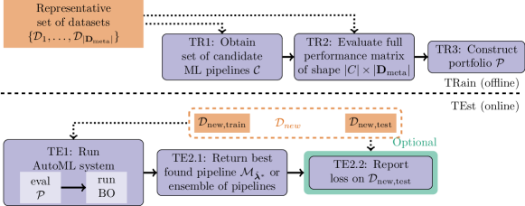
Figure 2: Schematic Overview of PoSH Auto-sklearn with the offline portfolio building phase (TR1-TR3) above and the test phase (TE1-TE2) below the dashed line. Rounded, purple boxes refer to computational steps while rectangular, orange boxes depict the input data to the AutoML system.

3.1.2 Theoretical Properties of the Greedy Algorithm

Besides the already mentioned practical advantages of the proposed greedy algorithm, this algorithm also enjoys a bounded worst-case error.

Proposition 1

Minimizing the test loss of a portfolio $\mathcal{P}$ on a set of datasets $\mathcal{D}_{1},\dots,\mathcal{D}_{|\mathbf{D}_{\text{meta}}|}$, when choosing an ML pipeline from $\mathcal{P}$ for $\mathcal{D}_{d}$ using holdout or cross-validation based on its performance on $\mathcal{D}_{d,\text{test}}$, is equivalent to the sensor placement problem for minimizing detection time (Krause et al., 2008).

We detail this equivalence in Appendix C.2. Thereby, we can apply existing results for the sensor placement problem to our problem. Using the test set of the meta-datasets $\mathbf{D}_{\text{meta}}$ to construct a portfolio is perfectly fine as long as we do not use new datasets $\mathcal{D}_{\text{new}}\in\mathbf{D}_{\text{test}}$ which we use for testing the approach.

Corollary 1

The penalty function for all meta-datasets is submodular.

We can directly apply the proof from Krause et al. (2008) that the so-called penalty function (i.e., maximum estimated generalization error minus the observed estimated generalization error) is submodular and monotone to our problem setup. Since linear combinations of submodular functions are also submodular (Krause and Golovin, 2014), the penalty function is also submodular.

Corollary 2

The problem of finding an optimal portfolio $\mathcal{P}^{*}$ is NP-hard (Nemhauser et al., 1978; Krause et al., 2008).

Corollary 3

Let $R$ denote the expected penalty reduction of a portfolio across all datasets, compared to the empty portfolio (which yields the worst possible score for each dataset). The greedy algorithm returns a portfolio $\mathcal{P}$ such that $R(\mathcal{P}^{*})\geq R(\mathcal{P})\geq(1-\frac{1}{e})R(\mathcal{P}^{*})$.

This means that the greedy algorithm closes at least 63% of the gap between the worst ADTM score (1.0) and the score the best possible portfolio $\mathcal{P}^{*}$ of size $|\mathcal{P}|$ would achieve (Nemhauser et al., 1978; Krause and Golovin, 2014). A generalization of this result given by Krause and Golovin (2014, Theorem 1.5) also tightens this bound to close 99% of the gap between the worst ADTM score and the score the optimal portfolio $\mathcal{P}^{*}$ of size $|\mathcal{P}^{*}|$ would achieve, by extending the portfolio constructed by the greedy algorithm to size $5\cdot|\mathcal{P}|$. Please note that a portfolio of size $5\cdot|\mathcal{P}|$ could be better than the optimal portfolio of size $|\mathcal{P}|$. This means that we can find a close-to-optimal portfolio on the meta-train datasets $\mathbf{D}_{\text{meta}}$ at the very least. Under the assumption that we apply the portfolio to datasets from the same distribution of datasets, we have a strong set of default ML pipelines.

We could also apply other strategies for the sensor set placement in our setting, such as mixed integer programming strategies, which can solve it optimally; however, these do not scale to portfolio sizes of a dozen ML pipelines (Krause et al., 2008; Pfisterer et al., 2018).

The same proposition (with the same proof) and corollaries apply if we select an ML pipeline based on an intermediate step in a learning curve or use cross-validation instead of holdout. We discuss using the validation set and other model selection and budget allocation strategies in Appendix C.3 and Appendix C.4.

3.2 Budget Allocation using Successive Halving

A key issue we identified during the last AutoML challenge was that training expensive configurations on the complete training set, combined with a low time budget, does not scale well to large datasets. At the same time, we noticed that our (then manual) strategy to run predefined pipelines on subsets of the data already yielded predictions good enough for ensemble building. This questions the common choice of assigning the same amount of resources to all pipeline evaluations, i.e. time, compute and data.

For this reason we introduce the principle of budget allocation strategies to AutoML, that describe how the resources are allocated to the pipeline evaluations. This is an orthogonal design decision to the model selection strategy, which approximates the generalization error of a single ML pipeline, and which is typically tackled by holdout or K-fold cross-validation (see Section 6.4.1).

As a principled alternative to always using the full budget, we used the successive halving bandit strategy (SH; Karnin et al., 2013; Jamieson and Talwalkar, 2016), which assigns more budget to promising machine learning pipelines and can easily be combined with iterative algorithms.

3.2.1 Approach

AutoML systems evaluate each pipeline under the same resource limitations and on the same budget (e.g., number of iterations using iterative algorithms). To increase efficiency for cases with tight resource limitations, we suggest allocating more resources to promising pipelines by using SH (Karnin et al., 2013; Jamieson and Talwalkar, 2016) to prune poor-performing pipelines aggressively.

Given a minimal and maximal budget per ML pipeline, SH starts by training a fixed number of ML pipelines for the smallest budget. Then, it iteratively selects $\frac{1}{\eta}$ of the pipelines with the lowest generalization error, multiplies their budget by $\eta$, and re-evaluates. This process is continued until only a single ML pipeline is left or the maximal budget is spent, and replaces the standard holdout procedure in which every ML pipeline is trained for the full budget.

While SH itself chooses new pipelines $\mathcal{M}_{\bm{\lambda}}$ to evaluate at random, we aim to extend on our work on Auto-sklearn 1.0 and continue to use BO. To do so, we follow work combining SH with BO (Falkner et al., 2018). Specifically, we use BO to iteratively suggest new ML pipelines $\mathcal{M}_{\bm{\lambda}}$, which we evaluate on the lowest budget until a fixed number of pipelines has been evaluated. Then, we run SH as described above. We are using Auto-sklearn’s standard random forest-based BO method SMAC and, according to the methodology of Falkner et al. (2018) build the model for BO on the highest available budget for which we have sufficient datapoints. While the original model had a mathematical requirement for $n+1$ finished pipelines, where $n$ is the number of hyperparameters to be optimized, the random forest model can guide the optimization with fewer datapoints, and we define sufficient as $\frac{n}{2}$. The portfolios we have introduced in Section 3.1 integrate seamlessly into this scheme: as long as not all members of the portfolio have been evaluated, we suggest them instead of asking BO for a new suggestion.

SH potentially provides large speedups, but it could also too aggressively cut away good configurations that need a higher budget to perform best. Thus, we expect SH to work best for large datasets, for which there is not enough time to train many ML pipelines for the full budget (FB), but for which training an ML pipeline on a small budget already yields a good indication of the generalization error.

We note that SH can be used in combination with both, holdout or cross-validation, and thus indeed adds another hyper-hyperparameter to the AutoML system, namely whether to use SH or FB. However, it also adds more flexibility to tackle a broader range of problems.

3.3 Practical Considerations and Challenge Results

In order to make best use of the successive halving algorithm we had to do certain adjustments to obtain high performance.

First, we restricted the search space to contain only iterative algorithms and no more feature preprocessing. This simplifies the usage of SH as we only have to deal with a single type of fidelity, the number of iterations, while we would otherwise have to also consider dataset subsets as an alternative. This leaves us with extremely randomized trees (Geurts et al., 2006), random forests (Breimann, 2001), histogram-based gradient boosting (Friedman, 2001; Ke et al., 2017), a linear model fitted with a passive aggressive algorithm (Crammer et al., 2006) or stochastic gradient descent and a multi-layer perceptron. The exact configuration space can be found in Table 18 of the appendix.

Second, because of using only iterative algorithms, we are able to store partially fitted models to disk to prevent having no predictions in case of time- and memouts. That is, after $2,4,8,\dots$ iterations, we make predictions for the validation set and dump the model for later usage. We provide further details, such as the restricted search space, in Appendix B.

For our submission to the second AutoML challenge, we implemented the following safeguards and tricks (Feurer et al., 2018), which we do not use in this paper since we instead focus on automatically designing a robust AutoML system:

• For the submission, we also employed support vector machines using subsets of the dataset as lower fidelities. Since none of the five final ensembles in the competition contained support vector machines, we did not consider them anymore for this paper, simplifying our methodology.

• We developed an additional library pruning method for ensemble selection. However, in preliminary experiments, we found that this, in the best case, provides an insignificant boost for the area under curve and not balanced accuracy, which we use in this work and thus did not follow up on that any further.

• To increase robustness against arbitrarily large datasets, we reduced all datasets to have at most $500$ features using univariate feature selection. Similarly, we also reduced all datasets to have at most $45\ 000$ datapoints using stratified subsampling. We do not think these are good strategies in general and only implemented them because we had no information about the dimensionality of the datasets used in the challenge, and to prevent running out of time and memory. Retrospectively, only one out of five datasets triggered this feature selection step. Now, we have instead a fallback strategy that is defined by data, see Section 4.1.1.

• In case the datasets had less than $1000$ datapoints, we would have reverted from holdout to cross-validation. However, this fallback was not triggered due to the datasets being larger in the competition.

• We manually added a linear regression fitted with stochastic gradient descent with its hyperparameters optimized for fast runtime as the first entry in the portfolio to maximize the chances of fitting a model within the given time. We had implemented this strategy because we did not know the time limit of the competition. However, as for the paper at hand and future applications of Auto-sklearn, we expect to know the optimization budget we are optimizing the portfolio for, we no longer require such a safeguard.

Our submission, PoSH Auto-sklearn, was the overall winner of the second AutoML challenge. We give the results of the competition in Table 1 and refer to Feurer et al. (2018) and Guyon et al. (2019) for further details, especially for information on our competitors.

Name	Rank	Dataset #1	Dataset #2	Dataset #3	Dataset #4	Dataset #5
PoSH Auto-sklearn	$\mathbf{2.8}$	$0.5533(3)$	$0.2839(4)$	$\mathbf{0.3932(1)}$	$\mathbf{0.2635(1)}$	$0.6766(5)$
narnars0	$3.8$	$0.5418(5)$	$0.2894(2)$	$0.3665(2)$	$0.2005(9)$	$\mathbf{0.6922(1)}$
Malik	$5.4$	$0.5085(7)$	$0.2297(7)$	$0.2670(6)$	$0.2413(5)$	$0.6853(2)$
wlWangl	$5.4$	$\mathbf{0.5655(2)}$	$\mathbf{0.4851(1)}$	$0.2829(5)$	$-0.0886(16)$	$0.6840(3)$
thanhdng	$5.4$	$0.5131(6)$	$0.2256(8)$	$0.2605(7)$	$0.2603(2)$	$0.6777(4)$

Table 1: Results for the second AutoML challenge (Guyon et al., 2019). Name is the team name, Rank the final rank of the submission, followed by the individual results on the five datasets used in the competition. All performances are the normalized area under the ROC curve (Guyon et al., 2015) with the per-dataset rank in brackets. In case a rank is missing, for example, rank 1 for dataset 1, this rank was achieved by a contestant who did not place within the top 5.

3.4 Experimental Setup

So far, AutoML systems were designed without any optimization budget or with a single, fixed optimization budget $T$ in mind (see Equation 5). Our system takes the optimization budget into account when constructing the portfolio. We will study two optimization budgets: a short, 10 minute optimization budget and a long, 60 minute optimization budget as in the original Auto-sklearn paper. To have a single metric for binary classification, multiclass classification and unbalanced datasets, we report the balanced error rate ($1-\text{balanced accuracy}$), following the 1${}^{\text{st}}$ AutoML challenge (Guyon et al., 2019). As different datasets can live on different scales, we apply a linear transformation to obtain comparable values. Concretely, we obtain the minimal and maximal error obtained by executing Auto-sklearn with portfolios and using ensembles for each combination of model selection and budget allocation strategies per dataset. Then, we rescale by subtracting the minimal error and dividing by the difference between the maximal and minimal error (ADTM, as introduced in Section 3.1.1). With this transformation, we obtain a normalized error which can be interpreted as the regret of our method.

We also limit the time and memory for each ML pipeline evaluation. For the time limit, we allow for at most $1/10$ of the optimization budget, while for the memory, we allow the pipeline 4GB before forcefully terminating the execution.

3.4.1 Datasets

We require two disjoint sets of datasets for our setup: (i) $\mathbf{D}_{\text{meta}}$, on which we build portfolios and the model-based policy selector that we will introduce in Section 4, and (ii) $\mathbf{D}_{\text{test}}$, on which we evaluate our method. The distribution of both sets ideally spans a wide variety of problem domains and dataset characteristics. For $\mathbf{D}_{\text{test}}$, we rely on $39$ datasets selected for the AutoML benchmark proposed by Gijsbers et al. (2019), which consists of datasets for comparing classifiers (Bischl et al., 2021) and datasets from the AutoML challenges (Guyon et al., 2019).

We collected the meta datasets $\mathbf{D}_{\text{meta}}$ based on OpenML (Vanschoren et al., 2014) using the OpenML-Python API (Feurer et al., 2021). To obtain a representative set, we considered all datasets on OpenML with more than $500$ and less than $1\,000\,000$ samples with at least two attributes. Next, we dropped all datasets that are sparse, contain time attributes or string type attributes as $\mathbf{D}_{\text{test}}{}$ does not contain any such datasets. Then, we dropped synthetic datasets and subsampled clusters of highly similar datasets. Finally, we manually checked for overlap with $\mathbf{D}_{\text{test}}$ and ended up with a total of $208$ training datasets and used them to train our method.

We show the distribution of the datasets in Figure 3. Green points refer to $\mathbf{D}_{\text{meta}}$ and orange crosses to $\mathbf{D}_{\text{test}}$. We can see that $\mathbf{D}_{\text{meta}}$ spans the underlying distribution of $\mathbf{D}_{\text{test}}$ quite well, but several datasets are outside the $\mathbf{D}_{\text{meta}}$ distribution indicated by the green lines, marked with a black cross. We give the full list of datasets for $\mathbf{D}_{\text{meta}}$ and $\mathbf{D}_{\text{test}}$ in Appendix E.

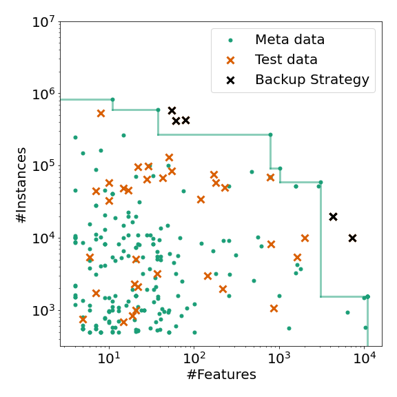
Figure 3: Distribution of meta and test datasets. We visualize each dataset w.r.t. its meta-features and highlight the datasets outside our meta distribution using black crosses.

For all datasets, we use a single holdout test set of $33.33\%$, which is defined by the corresponding OpenML task. The remaining $66.66\%$ are the training data of our AutoML systems, which handle further splits for model selection themselves based on the chosen model selection strategy.

3.4.2 Meta-data Generation

For each optimization budget we created four performance matrices of size $|\mathbf{D}_{\text{meta}}|\times|\mathcal{C}|$, see Section 3.1.1 for details on performance matrices. Each matrix refers to one way of assessing the generalization error of a model: holdout, 3-fold CV, 5-fold CV or 10-fold CV. To obtain each matrix, we did the following. For each dataset $\mathcal{D}$ in $\mathbf{D}_{\text{meta}}$, we used combined algorithm selection and hyperparameter optimization to find a customized ML pipeline. In practice, we ran Auto-sklearn without meta-learning and without ensemble building three times and picked the best resulting ML pipeline on the test split of $\mathcal{D}$. To ensure that Auto-sklearn finds a good configuration, we ran it for ten times the optimization budget given by the user (see Equation 5). Then, we ran the cross-product of all candidate ML pipelines and datasets to obtain the performance matrix. We also stored intermediate results for the iterative algorithms so that we could build custom portfolios for SH, too.

3.4.3 Other Experimental Details

We always report results averaged across $10$ repetitions to account for randomness and report the mean and standard deviation over these repetitions. To check whether performance differences are significant, where possible, we ran the Wilcoxon signed-rank test as a statistical hypothesis test with $\alpha=0.05$ (Demšar, 2006). In addition, we plot the average rank as follows. For each dataset, we draw one run per method (out of 10 repetitions) and rank these draws according to performance, using the average rank in case of ties. We then average over all 39 dataset and repeat this sampling $500$ times to and then plot the median and the 10th and 90th percentile of these samples. In the case of only three methods to compare, we can enumerate all $1000$ combinations of the seeds and do so. We use the exact method for Figure 6 and the sampling method for Figure 7 in the appendix.

We conducted all experiments using ensemble selection, and we constructed ensembles of size $50$ with replacement. We give results without ensemble selection in the Appendix B.2.

All experiments were conducted on a compute cluster with machines equipped with 2 Intel Xeon Gold 6242 CPUs with 2.8GHz (32 cores) and 192 GB RAM, running Ubuntu 20.04.01. We provide scripts for reproducing all our experimental results at https://github.com/automl/ASKL2.0_experiments and provide a clean integration of our methods into the official Auto-sklearn repository.

3.5 Experimental Results

In this subsection, we now validate the improvements for PoSH Auto-sklearn. First, we will compare using a portfolio to the previous KND approach and no warmstarting and second, we will compare PoSH Auto-sklearn to the previous Auto-sklearn 1.0.

	10 minutes			60 minutes
	BO	KND	Port	BO	KND	Port
FB; holdout	$5.98$	$5.29$	$\mathbf{3.70}$	$3.84$	$3.98$	$\mathbf{3.08}$
SH; holdout	$5.15$	$\underline{4.82}$	$\mathbf{4.11}$	$3.77$	$\underline{3.55}$	$\mathbf{3.19}$
FB; 3CV	$8.52$	$\underline{7.76}$	$\mathbf{6.90}$	$6.42$	$6.31$	$\mathbf{4.96}$
SH; 3CV	$7.82$	$7.67$	$\mathbf{6.16}$	$6.08$	$5.91$	$\mathbf{5.17}$
FB; 5CV	$9.48$	$9.45$	$\mathbf{7.93}$	$6.64$	$6.47$	$\mathbf{5.05}$
SH; 5CV	$9.48$	$\underline{8.85}$	$\mathbf{7.05}$	$6.19$	$5.83$	$\mathbf{5.40}$
FB; 10CV	$16.10$	$\underline{15.11}$	$\mathbf{12.42}$	$10.82$	$\underline{10.44}$	$\mathbf{9.68}$
SH; 10CV	$16.14$	$\underline{15.10}$	$\mathbf{12.61}$	$10.54$	$10.33$	$\mathbf{9.23}$

Table 2: Averaged normalized balanced error rate. We report the aggregated performance across $10$ repetitions and $39$ datasets of our AutoML system using only Bayesian optimization (BO), or BO warmstarted with k-nearest-datasets (KND) or a greedy portfolio (Port). Per line, we boldface the best mean value (per model selection and budget allocation strategy and optimization budget, and underline results that are not statistically different according to a Wilcoxon-signed-rank Test ($\alpha=0.05$)).

3.5.1 Portfolio vs. KND

Here, we study the performance of the learned portfolio and compare it against Auto-sklearn 1.0’s default meta-learning strategy using $25$ configurations. Additionally, we also study how pure BO would perform. We give results in Table 2.

For the new AutoML-hyperparameter $|\mathcal{P}|$, we chose $32$ to allow two full iterations of SH with our hyperparameter setting of SH. Unsurprisingly, warmstarting, in general, improves the performance on all optimization budgets and most model selection strategies, often by a large margin. The portfolios always improve over BO, while KND does so in all but one case. When comparing the portfolios to KND, we find that the raw results are always favorable and that for half of the settings, the differences are also significant.

3.5.2 PoSH Auto-sklearn vs Auto-sklearn 1.0

We can also look at the performance of PoSH Auto-sklearn compared to Auto-sklearn 1.0.

First, we compare the performance of PoSH Auto-sklearn to Auto-sklearn 1.0 using the full search space, and we provide those numbers in Table 3. For both time horizons, there is a strong reduction in the loss (10min: $16.21\rightarrow 4.11$ and 60min: $7.17\rightarrow 3.19$), indicating that the proposed PoSH Auto-sklearn is indeed an improvement over the existing solution and is able to fit better machine learning models in the given time limit.

		10MIN		60MIN
		$\varnothing$	std	$\varnothing$	std
(1)	PoSH-Auto-sklearn	$\mathbf{4.11}$	$0.09$	$\mathbf{3.19}$	$0.12$
(2)	Auto-sklearn (1.0)	$16.21$	$0.27$	$\underline{7.17}$	$0.30$

Table 3: Final performance of PoSH Auto-sklearn and Auto-sklearn 1.0. We report the normalized balanced error rate averaged across $10$ repetitions on $39$ datasets. We boldface the best mean value (per optimization budget) and underline results that are not statistically different according to a Wilcoxon signed-rank test ($\alpha=0.05$).

Second, we compare the performance of PoSH Auto-sklearn (SH; holdout and Port) to Auto-sklearn 1.0 (FB; holdout and KND) using only the reduced search space based on the results in Table 2. Again, there is a strong reduction in the loss for both time horizons (10min: $5.29\rightarrow 4.11$ and 60min: $3.98\rightarrow 3.19$), confirming abovementioned findings. Combined with the portfolio, the average results are inconclusive about whether our use of successive halving was the right choice or whether plain holdout would have been better. We also provide the raw numbers in Appendix B.3, but they are inconclusive, too.

4 Part II: Automating Design Decisions in AutoML

The goal of AutoML is to yield state-of-the-art performance without requiring the user to make low-level decisions, e.g., which model and hyperparameter configurations to apply. Using a portfolio and SH, PoSH Auto-sklearn is already an improvement over Auto-sklearn 1.0 in terms of efficiency and scalability. However, high-level design decisions, such as choosing between cross-validation and holdout or whether to use SH or not, remain. Thus, PoSH Auto-sklearn, and AutoML systems in general, suffer from a similar problem as they are trying to solve, as users have set their arguments on a per-dataset basis manually.

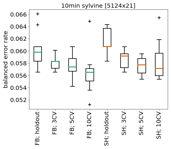
Figure 4: Final balanced error rate of BO using different model selection strategies averaged across $10$ repetitions. Top row: Results for a optimization budget of $10$ minutes on two different datasets. Bottom row: Results for a optimization budget of $10$ and $60$ minutes on the same dataset.

To highlight this dilemma, in Figure 4 we show exemplary results comparing the balanced error rates of the best ML pipeline found by searching our configuration space with BO using holdout, 3CV, 5CV and 10CV with SH and FB on different optimization budgets and datasets. The top row shows results obtained using the same optimization budget of $10$ minutes on two different datasets. While FB; 10CV is best on dataset sylvine (top left) the same strategy on median performs amongst the worst strategies on dataset adult (top right). Also, on sylvine, SH performs overall slightly worse in contrast to adult, where SH performs better on average. The bottom rows show how the given time-limit impacts the performance on the dataset jungle_chess_2pcs_raw_endgame_complete. Using a quite restrictive optimization budget of $10$ minutes (bottom left), SH; 3CV, which aggressively cuts ML pipelines on lower budgets, performs best on average. With a higher optimization budget (bottom right), the overall results improve and more strategies become competitive.

Therefore, we propose to extend AutoML systems with a policy selector to automatically choose an optimization policy given a dataset (see Figure 1 in Section 1 for a schematic overview). In this second part, we discuss the resulting approach, which led to Auto-sklearn 2.0 as the first implementation of it.

4.1 Automated Policy Selection

Specifically, we consider the case, where an AutoML system can be run with different optimization policies $\pi\in\Pi$ and study how to further automate AutoML using algorithm selection on this meta-meta level. In practice, we extend the formulation introduced in Equation 7 to not use an AutoML system $\mathcal{A}_{\pi}$ with a fixed policy $\pi$, but to contain a policy selector $\Xi:\mathcal{D}\rightarrow\pi$:

$$\savestack{\tmpbox}{\stretchto{\scaleto{\scalerel*[\widthof{GE}]{\kern-0.6pt\bigwedge\kern-0.6pt}{\rule[-614.295pt]{4.30554pt}{614.295pt}}}{}}{0.5ex}}\stackon[1pt]{GE}{\tmpbox}(\mathcal{A},\Xi,\mathbf{D}_{\text{meta}})=\frac{1}{\mid\mathbf{D}_{\text{meta}}\mid}\sum_{d=1}^{|\mathbf{D}_{\text{meta}}|}\savestack{\tmpbox}{\stretchto{\scaleto{\scalerel*[\widthof{GE}]{\kern-0.6pt\bigwedge\kern-0.6pt}{\rule[-614.295pt]{4.30554pt}{614.295pt}}}{}}{0.5ex}}\stackon[1pt]{GE}{\tmpbox}(\mathcal{A}_{\Xi(\mathcal{D}_{d})}(\mathcal{D}_{d}),\mathcal{D}_{d}).$$ (10)

In the remainder of this section, we describe how to construct such a policy selector.

4.1.1 Approach

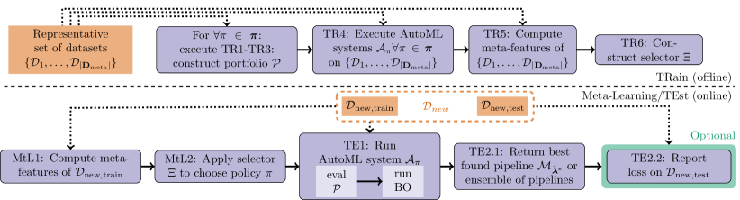
Figure 5: Schematic overview of the proposed Auto-sklearn 2.0 system with the training phase (TR1–TR6) above and the test phase (MtL1–MtL2&TE1–TE2) below the dashed line. Rounded, purple boxes refer to computational steps, while rectangular, orange boxes depict the input data to the AutoML system.

AutoML systems themselves are often heavily hyperparameterized. In our case, we deem the model selection strategy and budget allocation strategy (see Sections 3.2 and 6.4.1) as important choices the user has to make when using an AutoML system to obtain high performance. These decisions depend on both the given dataset and the available resources. As there is also an interaction between the two strategies and the optimal portfolio $\mathcal{P}$, we consider here that the optimization policy $\pi$ is parameterized by a combination of (i) model selection strategy, (ii) budget allocation strategy and (iii) a portfolio constructed for the choice of the two strategies. In our case, these are eight different policies ($\{$3-fold CV, 5-fold CV, 10-fold CV, holdout$\}\times\{$SH, FB$\}$).

We introduce a new layer on top of AutoML systems that automatically selects a policy $\pi$ for a new dataset. We show an overview of this system in Figure 5 which consists of a training (TR1–TR6) and a testing stage (MtL1–2 and TE1–TE2). In brief, in training steps TR1–TR3, we perform the same steps that we have already outlined in Figure 2. However, we now do so for each combination of model selection and budget allocation strategy. Our policies are combinations of a portfolio, a model selection strategy and a budget allocation strategy. We then execute the full AutoML system for each such policy in step TR4 to obtain a realistic performance estimate. In step TR5, we compute meta-features and use them together with the performance estimate from TR4 in step TR6 to train a model-based policy selector $\Xi$, which we will use in the online test phase.

In order to not overestimate the performance of $\pi$ on a dataset $\mathcal{D}_{d}$, dataset $\mathcal{D}_{d}$ must not be part of the meta-data for constructing the portfolio. To overcome this issue, we perform an inner 5-fold cross-validation and build each $\pi$ on four fifths of the meta-datasets $\mathbf{D}_{\text{meta}}$ and evaluate it on the left-out fifth of meta-datasets $\mathbf{D}_{\text{meta}}$. For the final AutoML system we then use a portfolio built on all meta-datasets $\mathbf{D}_{\text{meta}}$.

For a new dataset $\mathcal{D}_{\text{new}}\in\mathbf{D}_{\text{test}}{}$, we first compute meta-features describing $\mathcal{D}_{\text{new}}$ (MtL1) and use the model-based policy selector from step TR6 to automatically select an appropriate policy for $\mathcal{D}_{\text{new}}$ based on the meta-features (MtL2). This will relieve users from making this decision on their own. Given an optimization policy $\pi$, we then apply the AutoML system $\mathcal{A}_{\pi}$ to $\mathcal{D}_{\text{new}}$ (TE1). Finally, we return the best found pipeline $\mathcal{M}_{\hat{{\bm{\lambda}}}^{*}}$ based on the training set of $\mathcal{D}_{\text{new}}$ (TE2.1). Optionally, we can then compute the loss of $\mathcal{M}_{\hat{{\bm{\lambda}}}^{*}}$ on the test set of $\mathcal{D}_{\text{new}}$ (TE2.2); we emphasize that this would be the only time we ever access the test set of $\mathcal{D}_{\text{new}}$. Steps TE1–TE2 are the same as in Figure 2, and the only difference at evaluation time is that we use algorithm selection to decide which policy $\pi$ to use at test time instead of relying on a hand-picked one.

In the following, we describe two ways to construct a policy selector and introduce an additional backup strategy to make it robust towards failures.

Constructing the single best policy

A straightforward way to construct a selector relies on the assumption that the meta-datasets $\mathbf{D}_{\text{meta}}$ are homogeneous and that a new dataset is similar to these. In such a case, we can use per-set algorithm selection (Kerschke et al., 2019), which aims to find the single algorithm that performs best on average on a set of problem instances. In our context, it aims to find the combination of model selection and budget allocation that is best on average for the given set of meta-datasets $\mathbf{D}_{\text{meta}}$. This single best policy is then the automated replacement for our manual selection of SH and holdout in PoSH Auto-sklearn. While this seems to be a trivial baseline, it actually requires the same amount of compute power as the more elaborate strategy we introduce next.

Constructing the per-dataset Policy Selector

Instead of using a fixed, learned policy, we now propose to adapt the policy to the dataset at hand by using per-instance algorithm selection, which means we select the appropriate algorithm for each dataset by taking its properties into account. To construct the meta selection model (TR6), we follow the policy selector design of HydraMIP (Xu et al., 2011): for each pair of AutoML policies, we fit a random forest to predict whether policy $\pi_{A}$ outperforms policy $\pi_{B}$ given the current dataset’s meta-features. Since the misclassification loss depends on the difference between the losses of the two policies (i.e. the ADTM when choosing the wrong policy), we weight each meta-observation by their loss difference. To make errors comparable across different datasets (Bardenet et al., 2013), we scale the individual error values for each dataset. At test time (TE2), we query all pairwise models for the given meta-features and use voting for $\Xi$ to choose a policy $\pi$. We will refer to this strategy as the Policy Selector.

To improve the performance of the model-based policy selector, we applied BO to optimize the model-based policy selector’s hyperparameters to minimize the cross-validation error (Lindauer et al., 2015). We optimized in total seven hyperparameters, five of which are related to the random forest, one is how to combine the pairwise models to get a prediction, and the last one is the strategy of how to scale error values to compute weights for comparing datasets, i.e. using the raw observations, scale with $[min,max]$ / $[min,1]$ across a pair or all policies or use the difference in ranks as the weight (see Table 4). Hyperparameters are shared between all pairwise models to avoid factorial growth of the number of hyperparameters with the number of new model selection strategies. We allow a tree depth of 0, i.e., a tree with all data in a single leaf, which is equivalent to the single best strategy described above.

hyperparameter	type	values
Min. number of samples to create a further split	int	$[3,20]$
Min. number of samples to create a new leaf	int	$[2,20]$
Max. depth of a tree	int	$[0,20]$
Max. number of features to be used for a split	int	$[1,2]$
Bootstrapping in the random forest	cat	$\{yes,no\}$
Soft or hard voting when combining models	cat	$\{soft,hard\}$
Error value scaling to compute dataset weights	cat	see text

Table 4: configuration space of the model-based policy selector.

Meta-Features.

To train our model-based policy selector and to select a policy, as well to use the backup strategy, we use meta-features (Brazdil et al., 2008; Vanschoren, 2019) describing all meta-train datasets (TR5) and new datasets (TE1). To avoid the problems discussed in Section 3.1 we only use very simple and robust meta-features, which can be reliably computed in linear time for every dataset: 1) the number of datapoints and 2) the number of features. In fact, these are already stored as meta-data for the data structure holding the dataset. Using only these two meta-features for the selector can be regarded as learning the manually-designed fallbacks that we discussed in Section 3.3. In our experiments, we will show that even with only these trivial and cheap meta-features, we can substantially improve over a static policy.

Backup strategy.

Since there is no guarantee that our model-based policy selector will extrapolate well to datasets outside of the meta-datasets, we implement a fallback measure to avoid failures. Such failures can be harmful if a new dataset is, e.g., much larger than any dataset in the meta-dataset, and the model-based policy selector proposes to use a policy that would time out without any solution. More specifically, if there is no dataset in the meta-datasets that has higher or equal values for each meta-feature (i.e. dominates the dataset meta-features), our system falls back to use holdout with SH, which is the most aggressive and cheapest policy we consider. We visualize this in Figure 3 where we mark datasets outside our meta distribution using black crosses.

4.2 Experimental Results

		10MIN		60MIN
		$\varnothing$	std	$\varnothing$	std
(1)	Auto-sklearn (2.0)	$\mathbf{3.58}$	$0.23$	$\mathbf{2.47}$	$0.18$
(2)	PoSH-Auto-sklearn	$4.11$	$0.09$	$3.19$	$0.12$
(3)	Auto-sklearn (1.0)	$16.21$	$0.27$	$7.17$	$0.30$

Table 5: Average normalized balanced error (ADTM, lower is better) of Auto-sklearn 2.0, PoSH Auto-sklearn and Auto-sklearn 1.0 averaged across $10$ repetitions on $39$ datasets. We boldface the best mean value (per optimization budget) and underline results that are not statistically different according to a Wilcoxon-signed-rank Test ($\alpha=0.05$).

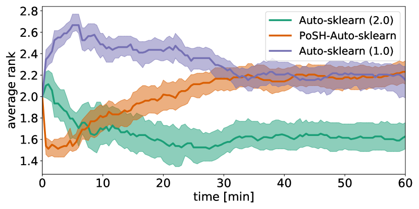
Figure 6: Performance over time. We report the median ranks (lower is better) and the 10th and 90th percentiles over time for Auto-sklearn 2.0 and the previous AutoML systems. Concretely, we compute the mean rank for for all $39{}$ for all $1000$ combinations of the $10$ seeds of the $3$ AutoML systems, and compute the median and percentiles of these $1000$ average ranks.

To study the performance of the policy selector, we compare it to PoSH Auto-sklearn as described in Section 3 and Auto-sklearn 1.0. From now on we refer to PoSH Auto-sklearn + policy selector as Auto-sklearn 2.0. As before, we study two horizons, $10$ minutes and $60$ minutes, and use versions of PoSH Auto-sklearn and Auto-sklearn 2.0 that were constructed with these time horizons in mind. Similarly, we use the same $208$ datasets for constructing our AutoML systems and the same $39$ for evaluating them.

Looking at Table 5, we see that Auto-sklearn 2.0 achieves the lowest error, being significantly better for both optimization budgets. Most notably, Auto-sklearn 2.0 reduces the relative error compared to Auto-sklearn 1.0 by $78\%$ (10MIN) and $65\%$, respectively, which means a reduction by a factor of $4.5$ and three.

It turns out that these results are skewed by several large datasets (task IDs 189873 and 75193 for both horizons; 189866, 189874, 168796 and 168797 only for the ten minutes horizon) on which the KND initialization of Auto-sklearn 1.0 only suggests ML pipelines that time out or hit the memory limit and thus exhaust the optimization budget for the full configuration space. Our new AutoML system does not suffer from this problem as it a) selects SH to avoid spending too much time on unpromising ML pipelines and b) can return predictions and results even if an ML pipeline was not evaluated for the full budget or converged early; and even after removing the datasets in question from the average, the performance of Auto-sklearn 1.0 is substantially worse than that Auto-sklearn 2.0.

When looking at the intermediate system, i.e. PoSH Auto-sklearn, we find that it outperforms Auto-sklearn 1.0 in terms of the normalized balanced error rate, but that the additional step of selecting the model selection and budget allocation strategy gives Auto-sklearn 2.0 an edge. When not considering the large datasets Auto-sklearn 1.0 failed on, their performance becomes very similar.

Figure 6 provides another view on the results, presenting average ranks (where failures obtain less weight compared to the averaged performance). Auto-sklearn 2.0 is still able to deliver best results, PoSH Auto-sklearn should be preferred to Auto-sklearn 1.0 for the first 30 minutes and then converges to roughly the same ranking.

4.3 Ablation

Now, we study the contribution of each of our improvements in an ablation study. We iteratively disable one component and compare the performance to the entire system using the $39$ datasets from the AutoML benchmark as done in the previous experimental sections. These components are (1) using a per-dataset model-based policy selector to choose a policy, (2) using only a subset of the available policies, and (3) warmstarting BO with a portfolio.

4.3.1 Do we need per-dataset selection?

We first examine how much performance we gain by having a model-based policy selector to decide between different AutoML strategies based on meta-features and how to construct this model-based policy selector, or whether it is sufficient to select a single strategy based on meta-training datasets. We compare the performance of the entire system using a model-based policy selector to using a single, static strategy (single best) and both, the model-based policy selector and the single best, without the fallback mechanism for out-of-distribution datasets and give all results in Table 6. We also provide two additional baselines: a random baseline, which randomly assigns a policy to a run and an oracle baseline, which marks the lowest possible error that can be achieved by any of the policies.

First, we compare the performance of the model-based policy selector with the single best. We can observe that for 10 minutes, there is a slight improvement in terms of performance, while the performance for 60 minutes is almost equal. While there is no significant difference to the single best for 10 minutes, there is for 60 minutes. These numbers can be compared with Table 2 to see how we fare against picking a single policy by hand. We find that our proposed algorithm selection compares favorably, especially for the longer time horizon.

Second, to study how much resources we need to spend on generating training data for our model-based policy selector, we consider three approaches: (P) only using the portfolio performance which we pre-computed and stored in the performance matrices as described in Section 3.1.1, (P+BO) actually running Auto-sklearn using the portfolio and BO for $10$ and $60$ minutes, respectively, and (P+BO+E) additionally also constructing ensembles, which yields the most realistic meta-data. Running BO on all $208$ datasets (P+BO) is by far more expensive than the table lookups (P); building an ensemble (P+BO+E) adds only several seconds to minutes on top compared to (P+BO).

For both optimization budgets using P+BO yields the best results using the model-based policy selector closely followed by P+BO+ENS, see Table 6. The cheapest method, P, yields the worst results showing that it is worth investing resources into computing good meta-data. Surprisingly, looking at the single best, performance gets worse when using seemingly better meta-data. We investigated the reason why P+BO performs slightly better than P+BO+ENS. When using a model-based policy selector, this can be explained by a single dataset for both time horizons for which the policy chosen by the model-based policy selector is worse than the single best policy. When looking at the single best, there is no single dataset which stands out. To summarize, investing additional resources to compute realistic meta-data results in improved performance, but so far, it appears that having the effect of BO in the meta-data is sufficient, while the ensemble seems to lead to lower meta-data quality.

	10 Min			60 Min
trained on	P	P+BO	P+BO+E	P	P+BO	P+BO+E
model-based policy selector	$\underline{3.58}$	3.56	$\underline{3.58}$	$2.53$	2.32	$\underline{2.47}$
model-based policy selector w/o fallback	$\underline{5.43}$	$\underline{5.68}$	$\underline{4.79}$	$4.98$	$5.36$	$\underline{5.43}$
single best	$3.88$	$\underline{3.67}$	$\underline{3.69}$	$2.49$	$\underline{2.38}$	$2.44$
single best w/o fallback	$5.18$	$\underline{6.38}$	$\underline{6.40}$	$5.10$	$5.01$	$5.07$
oracle	$2.33$			$1.22$
random	$8.32$			$6.18$

Table 6: Average normalized balanced error (ADTM, lower is better) for $10$ and $60$ minutes. We report the performance for the model-based policy selector policy and the single best when trained on different data obtained on $\mathbf{D}_{\text{meta}}{}$ (P = Portfolio, BO = Bayesian Optimization, E = Ensemble) as well as the model-based policy selector without the fallback. The second part of the table shows the results of always choosing the best policy on the test set (oracle) and results for choosing a random policy (random) as baselines. We boldface the best mean value (per optimization budget) and underline results that are not statistically different according to a Wilcoxon-signed-rank Test ($\alpha=0.05$).

Finally, we also take a closer look at the impact of the fallback mechanism to verify that our improvements are not solely due to this component. We observe that the performance drops for all policy selection strategies that do not use the fallback mechanism. For the shorter 10 minutes setting, we find that the model-based policy selector still outperforms the single best, while for the longer 60 minutes setting, the single best leads to better performance. The rather stark performance degradation compared to the regular model-based policy selector can mainly be explained by a few, huge datasets, to which the model-based policy selector cannot extrapolate (and which the single best does not account for). Based on these observations, we suggest research into an adaptive fallback strategy that can change the model selection strategy during the execution of the AutoML system so that a policy selector can be used on out-of-distribution datasets. We conclude that using a model-based policy selector is beneficial, and using a fallback strategy to cope with out-of-distribution datasets can substantially improve performance.

4.3.2 Do we need different model selection strategies?

		Selector		Random		Oracle
		$\varnothing$	std	$\varnothing$	std	$\varnothing$	std
10 Min	All	3.58	0.23	7.46	2.02	2.33	0.06
	Only Holdout	4.03	0.14	3.78	0.23	3.23	0.10
	Only CV	6.11	0.11	8.66	0.70	5.28	0.06
	Only FB	3.50	0.20	7.64	2.00	2.59	0.09
	Only SH	3.63	0.19	6.95	1.98	2.75	0.07
60 Min	All	2.47	0.18	5.64	1.95	1.22	0.08
	Only Holdout	3.18	0.15	3.13	0.12	2.62	0.07
	Only CV	5.09	0.19	6.85	0.86	3.94	0.10
	Only FB	2.39	0.18	5.46	1.52	1.51	0.06
	Only SH	2.44	0.24	5.13	1.72	1.68	0.12

Table 7: Average Normalized balanced error (ADTM, lower is better) for the full system and when not considering all model selection strategies.

Next, we study whether we need the different model selection strategies. For this, we build model-based policy selectors on different subsets of the available eight combinations of model selection strategies and budget allocations: $\{$3-fold CV, 5-fold CV, 10-fold CV, holdout$\}\times\{$SH, FB$\}$. Only Holdout consists of holdout with SH or FB (2 combinations), Only CV comprises 3-fold CV, 5-fold CV and 10-fold CV, all of them with SH or FB (6 combinations), FB contains both holdout and cross-validation and assigns each pipeline evaluation the same budget (4 combinations) and Only SH uses SH to assign budgets (4 combinations).

In Table 7, we compare the performance of selecting a policy at random (random), the performance of selecting the best policy on the test set and thus giving a lower bound on the ADTM (oracle) and our model-based policy selector. The oracle indicates the best possible performance with each of these subsets of model selection strategies. It turns out that both Only Holdout and Only CV have a much worse oracle performance than All, with the oracle performance of Only CV being even worse than the performance of the model-based policy selector for All. Looking at Full budget (FB), it turns out that this subset would be slightly preferable in terms of performance with a policy selector. However, the oracle performance is worse than that of All which shows that there is some complementarity between the different policies which cannot yet be exploited by the policy selector. For Only Holdout, surprisingly, the random policy selector performs slightly better than the model-based policy selector. We attribute this to the fact that holdout with both SH and FB performs similarly and that the choice between these two cannot yet be learned, possibly also indicated by the close performance of the random selector.

These results show that a large variety of available model selection strategies to choose from increases best possible performances. However, they also show that a model-based policy selector cannot yet necessarily leverage this potential. This questions the usefulness of choosing from all model selection strategies, similar to a recent finding which proves that increasing the number of different policies a policy selector can choose from leads to reduced generalization (Balcan et al., 2021). However, we believe this points to the research question of whether we can learn on the meta-datasets which model selection and budget allocation strategies to include in the set of strategies to choose from. Also, with an ever-growing availability of meta-datasets and continued research on robust policy selectors, we expect this flexibility to eventually yield improved performance.

4.3.3 Do we still need to warm-start Bayesian optimization?

		10min		60min
		$\varnothing$	std	$\varnothing$	std
With Portfolio	Policy selector	3.58	0.23	2.47	0.18
	Single best	3.69	0.14	2.44	0.12
Without Portfolio	Policy selector	5.63	0.89	3.42	0.32
	Single best	5.37	0.58	3.61	0.61

Table 8: Average normalized balanced error (ADTM, lower is better) after $10$ and after $60$ minutes with portfolios (top) and without (bottom). The row ”with portfolio” and ”policy selector” constitutes the full AutoML system including portfolios, BO and ensembles) and the row ”without portfolios” and ”policy selector” only removes the portfolios (both from the meta-data for model-based policy selector construction and at runtime). We boldface the best mean value (per optimization budget) and underline results that are not statistically different according to a Wilcoxon-signed-rank Test ($\alpha=0.05$).

Last, we analyze the impact of the portfolio. Given the other improvements, we now discuss whether we still need to add the additional complexity and invest resources to warm-start BO (and can therefore save the time to build the performance matrices to construct the portfolios). For this study, we completely remove the portfolio from our AutoML system, meaning that we directly start with BO and construct ensembles – both for creating the data we train our policy selector on and for reporting performance. We report the results in Table 8.

Comparing the performance of an AutoML system with a model-based policy selector with and without portfolios (Row 1 and 3), there is a clear drop in performance when disabling the portfolios. Comparing Rows 2 and 4 also demonstrates that a portfolio is necessary when using the single best policy. This ablation highlights the importance of initializing the search procedure of AutoML systems with well-performing pipelines.

5 Comparison to other AutoML systems

Having established that Auto-sklearn 2.0 does indeed improve over Auto-sklearn 1.0, we now compare our system to other well established AutoML systems. For this, we use the publicly available AutoML benchmark suite which defines a fixed benchmarking environment for AutoML systems (Gijsbers et al., 2019) comparisons. We use the original implementation of the benchmark and compare Auto-sklearn 1.0 and Auto-sklearn 2.0 to the provided implementations of Auto-WEKA (Thornton et al., 2013), TPOT (Olson et al., 2016a, b), H2O AutoML (LeDell and Poirier, 2020) and a random forest baseline with hyperparameter tuning on $39$ datasets as implemented by the benchmark suite. These $39$ datasets are the same datasets as in $\mathbf{D}_{\text{test}}$ and we provide details in Table 20 in the appendix.

5.1 Integration and setup

To avoid hardware-dependent performance differences, we (re-)ran all AutoML systems on our local hardware (see Section 3.4.3). We used the pre-defined 1h8c setting, which divides each dataset into ten folds and gives each framework one hour on eight CPU cores to produce a final model. We furthermore assigned each run $32$GB of RAM, which a SLURM cluster manager controlls. In addition, we conducted five repeats to account for randomness. The benchmark comes with Docker containers (Merkel, 2014). However, Docker requires superuser access on the execution nodes, which is not available on our compute cluster. Therefore, we extended the AutoML benchmark with support for Singularity images (Kurtzer et al., 2017), and used them to isolate the framework installations from each other. For reproducibility, we give the exact versions we used in Table 17 in the Appendix.

The default resource allocation of the AutoML benchmark is a highly parallel setting with eight cores. We chose the most straightforward way of making use of these resources for Auto-sklearn and evaluated eight ML pipelines in parallel, assigning each $total\_memory/num\_cores$ RAM, which are $4$GB. This allows us to evaluate configurations obtained from the portfolio or KND in parallel but also requires a parallel strategy for running BO afterwards. We extended the Bayesian optimization package SMAC3 (Lindauer et al., 2022) to allow for asynchronous parallel optimization. In preliminary experiments, we found that the inherent randomness of the random forest used by SMAC combined with the interleaved random search of SMAC is sufficient to obtain results that perform a lot better than the previous parallelism implemented in Auto-sklearn via SMAC (Ramage, 2015). Whenever a pipeline finishes training, Auto-sklearn checks whether there is an instance of the ensemble construction running, and if not, it uses one of the eight slots to conduct ensemble building and otherwise continues to fit a new pipeline. We implemented this version of parallel Auto-sklearn using Dask (Dask Development Team, 2016).

5.2 Results

	AS 2.0	AS 1.0	AW	TPOT	H2O	TunedRF
adult	$0.0692$	$0.0701$	$0.0920$	$0.0750$	$\mathbf{0.0690}$	$0.0902$
airlines	$0.2724$	$0.2726$	$0.3241$	$0.2758$	$\mathbf{0.2682}$	-
albert	$0.2413$	$\mathbf{0.2381}$	-	$0.2681$	$0.2530$	$0.2616$
amazon	$0.1233$	$0.1412$	$0.1836$	$0.1345$	$\mathbf{0.1218}$	$0.1377$
apsfailure	$0.0085$	$\mathbf{0.0081}$	$0.0365$	$0.0099$	$0.0081$	$0.0087$
australian	$\mathbf{0.0594}$	$0.0702$	$0.0709$	$0.0670$	$0.0607$	$0.0610$
bank-marketing	$\mathbf{0.0607}$	$0.0616$	$0.1441$	$0.0664$	$0.0610$	$0.0692$
blood-transfusion	$\mathbf{0.2428}$	$0.2474$	$0.2619$	$0.2761$	$0.2430$	$0.3122$
car	$\mathbf{0.0012}$	$0.0046$	$0.1910$	$2.7843$	$0.0032$	$0.0421$
christine	$0.1821$	$\mathbf{0.1703}$	$0.2026$	$0.1821$	$0.1763$	$0.1908$
cnae-9	$\mathbf{0.1424}$	$0.1779$	$0.7045$	$0.1483$	$0.1807$	$0.3119$
connect-4	$0.3387$	$0.3535$	$1.7083$	$0.3856$	$\mathbf{0.3127}$	$0.4777$
covertype	$\mathbf{0.1103}$	$0.1435$	$3.3515$	$0.5332$	$0.1281$	-
credit-g	$0.2031$	$0.2159$	$0.2505$	$0.2144$	$0.2078$	$\mathbf{0.1985}$
dilbert	$0.0399$	$\mathbf{0.0332}$	$2.0791$	$0.1153$	$0.0359$	$0.3283$
dionis	$\mathbf{0.5620}$	$0.7171$	-	-	$4.7758$	-
fabert	$0.7386$	$0.7466$	$5.4784$	$0.8431$	$\mathbf{0.7274}$	$0.8060$
fashion-mnist	$\mathbf{0.2511}$	$0.2524$	$0.9505$	$0.4314$	$0.2762$	$0.3613$
guillermo	$0.0945$	$\mathbf{0.0871}$	$0.1251$	$0.1680$	$0.0911$	$0.0973$
helena	$\mathbf{2.4974}$	$2.5432$	$14.3523$	$2.8738$	$2.7578$	-
higgs	$\mathbf{0.1824}$	$0.1846$	$0.3379$	$0.1969$	$0.1846$	$0.1966$
jannis	$0.6709$	$\mathbf{0.6637}$	$2.9576$	$0.7244$	$0.6695$	$0.7288$
jasmine	$0.1141$	$0.1196$	$0.1356$	$0.1123$	$0.1141$	$\mathbf{0.1118}$
jungle_chess	$0.2104$	$0.1956$	$1.6969$	$0.9557$	$\mathbf{0.1479}$	$0.4020$
kc1	$0.1611$	$0.1594$	$0.1780$	$\mathbf{0.1530}$	$0.1745$	$0.1590$
kddcup09	$\mathbf{0.1580}$	$0.1632$	-	$0.1696$	$0.1636$	$0.2058$
kr-vs-kp	$\mathbf{0.0001}$	$0.0003$	$0.0217$	$0.0003$	$0.0002$	$0.0004$
mfeat-factors	$\mathbf{0.0726}$	$0.0901$	$0.5678$	$0.1049$	$0.1009$	$0.2091$
miniboone	$\mathbf{0.0121}$	$0.0128$	$0.0352$	$0.0177$	$0.0129$	$0.0183$
nomao	$\mathbf{0.0035}$	$0.0039$	$0.0157$	$0.0047$	$0.0036$	$0.0049$
numerai28.6	$0.4696$	$0.4705$	$0.4729$	$0.4741$	$\mathbf{0.4695}$	$0.4792$
phoneme	$\mathbf{0.0299}$	$0.0366$	$0.0416$	$0.0307$	$0.0325$	$0.0347$
riccardo	$0.0002$	$\mathbf{0.0002}$	$0.0020$	$0.0021$	$0.0003$	$0.0002$
robert	$1.4302$	$\mathbf{1.3800}$	-	$1.8600$	$1.4927$	$1.6877$
segment	$\mathbf{0.1482}$	$0.1749$	$1.2497$	$0.1660$	$0.1580$	$0.1718$
shuttle	$\mathbf{0.0002}$	$0.0004$	$0.0100$	$0.0008$	$0.0004$	$0.0006$
sylvine	$0.0105$	$0.0091$	$0.0290$	$\mathbf{0.0075}$	$0.0106$	$0.0159$
vehicle	$0.3341$	$0.3754$	$2.0662$	$0.4402$	$\mathbf{0.3067}$	$0.4839$
volkert	$\mathbf{0.7477}$	$0.7862$	$3.4235$	$0.9852$	$0.8121$	$0.9792$
Rank	$\mathbf{1.79}$	$2.64$	$5.72$	$4.08$	$2.38$	$4.38$
Best performance	$\mathbf{19}$	$8$	$0$	$2$	$8$	$2$
Wins/Losses/Ties of AS 2.0	-	$28/11/0$	$39/0/0$	$35/4/0$	$26/13/0$	$36/3/0$
P-values (AS 2.0 vs. other methods),	-	$.009$	$<.000$	$<.000$	$.053$	$<.000$
based on a Binomial sign test

Table 9: Results of the AutoML benchmark averaged across five repetitions. We report log loss for multiclass datasets and $1-AUC$ for binary classification datasets (lower is better). AS is short for Auto-sklearn and AW for Auto-WEKA. Auto-sklearn has the best overall rank, the best performance in most datasets and, based on the P-values of a Binomial sign test, we gain further confidence in its strong performance.

We give results for the AutoML benchmark in Table 9. For each dataset, we give the average performance of the AutoML systems across all ten folds and five repetitions and boldface the one with the lowest error (we cannot give any information about whether differences are significant as we cannot compute significances on cross-validation folds as described by Bengio and Grandvalet, 2004).

We report the log loss for multiclass datasets and $1-AUC$ for binary datasets (lower is better). In addition, we provide the average rank as an aggregate measure (computed by averaging all folds and repetitions per dataset and then computing the rank). Furthermore, we count how often each framework is the winner on a dataset (champion), and give the losses, wins and ties against Auto-sklearn 2.0. We then use these to perform a binomial sign test (Demšar, 2006) to compare the individual algorithms against Auto-sklearn 2.0.

The results in Table 9 show that none of the AutoML systems is best on all datasets, and even the TunedRF performs best on a few datasets. However, we can also observe that the proposed Auto-sklearn 2.0 has the lowest average rank. It is followed by H2O AutoML and Auto-sklearn 1.0 which perform roughly en par wrt the ranking scores and the number of times they are the winner on a dataset. According to both aggregate metrics, the TunedRF, Auto-WEKA and TPOT cannot keep up and lead to substantially worse results. Finally, both versions of Auto-sklearn appear to be quite robust as they reliably provide results on all datasets, including the largest ones where several of the other methods fail.

6 Related Work

We now present related work on our individual contributions (portfolios, model selection strategies, and algorithm selection) as well as on related AutoML systems.

6.1 Related Work on Portfolios

Portfolios were introduced for hard combinatorial optimization problems, where the runtime between different algorithms varies drastically and allocating time shares to multiple algorithms instead of allocating all available time to a single one reduces the average cost for solving a problem (Huberman et al., 1997; Gomes and Selman, 2001), and had applications in different sub-fields of AI (Smith-Miles, 2008; Kotthoff, 2014; Kerschke et al., 2019). Algorithm portfolios were introduced to ML by the name of algorithm ranking to reduce the required time to perform model selection compared to running all algorithms under consideration (Brazdil and Soares, 2000; Soares and Brazdil, 2000), ignoring redundant ones (Brazdil et al., 2001). ML portfolios can be superior to hyperparameter optimization with Bayesian optimization (Wistuba et al., 2015b), Bayesian optimization with a model which takes past performance data into account (Wistuba et al., 2015a) or can be applied when there is simply no time to perform full hyperparameter optimization (Feurer et al., 2018). Furthermore, such a portfolio-based model-free optimization is both easier to implement than regular Bayesian optimization and meta-feature based solutions, and the portfolio can be shared easily across researchers and practitioners without the necessity of sharing meta-data (Wistuba et al., 2015a, b; Pfisterer et al., 2018) or additional hyperparameter optimization software. Here, our goal is to have strong hyperparameter settings when there is no time to optimize with a typical black-box algorithm.

The efficient creation of algorithm portfolios is an active area of research with the Greedy Algorithm being a popular choice (Xu et al., 2010, 2011; Seipp et al., 2015; Wistuba et al., 2015b; Lindauer et al., 2017; Feurer et al., 2018; Feurer and Hutter, 2018) due to its simplicity. Wistuba et al. (2015b) first proposed the use of the Greedy Algorithm for pipelines of ML portfolios, minimizing the average rank on meta-datasets for a single ML algorithm. Later, they extended their work to update the members of a portfolio in a round-robin fashion, this time using the average normalized misclassification error as a loss function and relying on a Gaussian process model (Wistuba et al., 2015a). The loss function of the first method does not optimize the metric of interest, while the second method requires a model and does not guarantee that well-performing algorithms are executed early on, which could be harmful under time constraints.

Research into the Greedy Algorithm continued after our submission to the second AutoML challenge and the publication of the employed methods (Feurer et al., 2018). Pfisterer et al. (2018) suggested using a set of default values to simplify hyperparameter optimization. They argued that constructing an optimal portfolio of hyperparameter settings is a generalization of the Maximum coverage problem and propose two solutions based on Mixed Integer Programming and the Greedy Algorithm which we also use as the base of our algorithm. The greedy algorithm recently also drew interest in deep learning research, where it was applied in its basic form for tuning the hyperparameters of the popular ADAM algorithm (Metz et al., 2020).

Extending these portfolio strategies, which are learned offline, there are online portfolios that can select from a fixed set of machine learning pipelines, taking previous evaluations into account (Leite et al., 2012; Wistuba et al., 2015a, b; Fusi et al., 2018; Yang et al., 2019, 2020). However, such methods cannot be directly combined with all budget allocation strategies as they require the definition of a special model for extrapolating learning curves (Klein et al., 2017b; Falkner et al., 2018) and also introduce additional complexity into AutoML systems.

There exists other work on building portfolios without prior discretization (which we do for our work and was done for most work mentioned above), which directly optimizes the hyperparameters of ML pipelines to add next to the portfolio in a greedy fashion (Xu et al., 2010, 2011; Seipp et al., 2015), to jointly optimize all configurations of the portfolio with global optimization (Winkelmolen et al., 2020), and also to build parallel portfolios (Lindauer et al., 2017). We consider these to be orthogonal to using portfolios in the first place and plan to study improved optimization strategies in future work.

6.2 Related Work on Successive Halving

Large datasets, expensive ML pipelines and tight resource limitations demand sophisticated methods to speed up pipeline selection. One line of research, multi-fidelity optimization methods, tackle this problem by using cheaper approximations of the objective of interest. Practical examples are evaluating a pipeline only on a subset of the dataset or for iterative algorithms limiting the number of iterations. There exists a large body of research on optimization methods leveraging lower fidelities, for example working with a fixed set of auxiliary tasks (Forrester et al., 2007; Swersky et al., 2013; Poloczek et al., 2017; Moss et al., 2020), solutions for specific model classes (Swersky et al., 2014; Domhan et al., 2015; Chandrashekaran and Lane, 2017) and selecting a fidelity value from a continuous range (Klein et al., 2017a; Kandasamy et al., 2017; Wu et al., 2020; Takeno et al., 2020). Here, we focus on a methodologically simple bandit strategy, SH (Karnin et al., 2013; Jamieson and Talwalkar, 2016), which successively reduces the number of candidates and at the same time increases the allocated resources per run till only one candidate remains. Our use of SH in the 2nd AutoML challenge also inspired work on combining a genetic algorithm with SH (Parmentier et al., 2019). Another way of quickly discarding unpromising pipelines is the intensify procedure which was used by Auto-WEKA (Thornton et al., 2013) to speed up cross-validation. Instead of evaluating all folds at once, it evaluates the folds in an iterative fashion. After each evaluation, the average performance on the evaluated folds is compared to the performance of the so-far best pipeline on these folds. The evaluation is only continued if the performance is equal or better. While this allows evaluating many configurations in a short time, it cannot be combined with post-hoc ensembling and reduces the cost of a pipeline to, at most, the cost of holdout, which might already be too high.

6.3 Related Work on Algorithm Selection

Automatically choosing a model selection strategy to assess the performance of an ML pipeline for hyperparameter optimization has not previously been tackled, and only Guyon et al. (2015) acknowledge the lack of such an approach. However, treating the choice of model selection strategy as an algorithm selection problem allows us to apply methods from the field of algorithm selection (Smith-Miles, 2008; Kotthoff, 2014; Kerschke et al., 2019) and we can in future work reuse existing techniques besides the pairwise classification we employ in this paper (Xu et al., 2011), such as the AutoAI system AutoFolio (Lindauer et al., 2015).

6.4 Background on AutoML Systems and Their Components

AutoML systems have recently gained traction in the research community, and there exists a multitude of approaches, often accompanied by open-source software. In the following, we provide background on the main components of AutoML frameworks before describing several prominent instantiations in more depth.

6.4.1 Components of AutoML systems

AutoML systems require a flexible pipeline configuration space and are driven by an efficient method to search this space. Furthermore, they rely on model selection and budget allocation strategies when evaluating different pipelines. Additionally, to speed up the search procedure, information gained on other datasets can be used to kick-start or guide the search procedure (i.e. meta-learning). Finally, one can also combine the models trained during the search phase in a post-hoc ensembling step.

Configuration Space and Search Mechanism

While there are configuration space formulations that allow the application of multiple search mechanisms, not all formulations of a configuration space and a search mechanism can be mixed and matched, and we, therefore, describe the different formulations and the applicable search mechanisms in turn.

The most common description of the search space is the CASH formulation. There is a fixed amount of hyperparameters, each with a range of legal values or categorical choices, and some of them can be conditional, meaning that they are only active if other hyperparameters fulfill certain conditions. One such example is the choice of a classification algorithm and its hyperparameters. The hyperparameters of an SVM are only active if the categorical hyperparameter of the classification algorithm is set to SVM.

Standard black-box optimization algorithms can solve the CASH problem, and SMAC (Hutter et al., 2011) and TPE (Bergstra et al., 2011) were proposed first for this task. Others proposed the use of evolutionary algorithms (Bürger and Pauli, 2015) and random search (LeDell and Poirier, 2020). It is also known as the full model selection problem (Escalante et al., 2009), and solutions in that strain of work proposed the use of particle swarm optimization (Escalante et al., 2009) and a combination of a genetic algorithm with particle swarm optimization (Sun et al., 2013). To improve performance one can prune the configuration space to reduce the size of the space the optimization algorithm has to search through (Zhang et al., 2016), split the configuration space into smaller, more manageable subspaces (Alaa and van der Schaar, 2018; Liu et al., 2020), or heavily employ expert knowledge (LeDell and Poirier, 2020).

Instead of a fixed configuration space, genetic programming can make use of a flexible and possibly infinite space of components to be connected (Olson et al., 2016b, a). This approach can be formalized further by using grammar-based genetic programming (de Sa et al., 2017). Context-free grammars can also be searched by model-based reinforcement learning algorithms (Drori et al., 2019).

Formalizing the search problem as a search tree allows the application of a custom Monte-Carlo tree search (Rakotoarison et al., 2019) and hierarchical task networks with best-first search (Mohr et al., 2018). With discrete spaces it is also possible to use combinations of meta-learning and matrix factorization (Yang et al., 2019, 2020; Fusi et al., 2018). In the special case of using only neural networks in an AutoML system it is possible to stick with standard black-box optimization (Mendoza et al., 2016, 2019; Zimmer et al., 2021), but one can also employ recent advances in neural architecture search (Elsken et al., 2019).

Meta-Learning.

When there is knowledge about previous runs of the AutoML system on other datasets available, it is possible to employ meta-learning. One option is to define a dataset similarity measure, often by using hand-crafted meta-features which describe the datasets (Brazdil et al., 1994), to use the best solutions on the closest seen datasets to warmstart the search algorithm (Feurer et al., 2015a). While this way of meta-learning can be seen as an add-on to existing methods, other works use search strategies designed to take meta-learning into account, for example matrix factorization (Yang et al., 2019, 2020; Fusi et al., 2018) or reinforcement learning (Drori et al., 2019; Heffetz et al., 2020).

Model Selection.

Given training data, the goal of an AutoML system is to find the best performing ML pipeline. Doing so requires to best approximate the generalization error to 1) provide a reliable and precise signal for the optimization procedure and 2) select the model to be returned in the end. Typically, the generalization error is assessed via the train-validation-test protocol (Bishop, 1995; Raschka, 2018). This means that several models are trained on a training set, the best one is selected via holdout (using a single split) or the K-fold cross-validation, and the generalization error is then reported on the test set. The AutoML system then returns a single model in case of holdout and a combination of $K$ models in case of $K$-fold cross-validation (Caruana et al., 2006). One could also use model selection strategies aiming to reduce the effect of overfitting to the validation set (Dwork et al., 2015; Tsamardinos et al., 2018), but while such model selection strategies are an important area of research, houldout or K-fold cross-validation remain the most prominent choices (Henery, 1994; Kohavi and John, 1995; Hastie et al., 2001; Guyon et al., 2010; Bischl et al., 2012; Raschka, 2018).

The influence of the model selection strategy on the performance is well known (Kalousis and Hilario, 2003), and researchers have studied their impact (Kohavi, 1995). However, there is no single best strategy, since there is a tradeoff between approximation quality and time required to compute the validation loss.

Post-hoc Ensembling.

AutoML systems evaluate dozens or hundreds of models during their optimization procedure. Thus, it is a natural next step to not only use a single model at the end but to ensemble multiple for improved performance and reduced overfitting.

This was first proposed to combine the solutions found by particle swarm optimization (Escalante et al., 2010) and then by an evolutionary algorithm (Bürger and Pauli, 2015). While these works used heuristic methods to combine multiple models into a final ensemble, it is also possible to treat this as another optimization problem (Feurer et al., 2015a) and solve it with ensemble selection (Caruana et al., 2004) or stacking (LeDell and Poirier, 2020).

Instead of using a single layer of machine learning models, Automatic Frankensteining (Wistuba et al., 2017) proposed two-layer stacking, applying AutoML to the outputs of an AutoML system instead of a single layer of ML algorithms followed by an ensembling mechanism. Auto-Stacker went one step further, directly optimizing for a two-layer AutoML system (Chen et al., 2018).

6.4.2 AutoML systems

To the best of our knowledge, the first AutoML system which tunes both hyperparameters and chooses algorithms was an ensemble method (Caruana et al., 2004). This system randomly produces $2\ 000$ classifiers from a wide range of ML algorithms and constructs a post-hoc ensemble. It was later robustified (Caruana et al., 2006) and employed in a winning submission to the KDD challenge (Niculescu-Mizil et al., 2009).

The first AutoML system to jointly optimize the whole pipeline was Particle Swarm Model Selection (Escalante et al., 2007, 2009). It used a fixed-length representation of the pipeline and contained feature selection, feature processing, classification and post-processing implemented in the CLOP package and was developed for the IJCNN 2007 agnostic learning vs. prior knowledge challenge (Guyon et al., 2007). It placed 2nd among the solutions using the CLOP package provided by the organizers, only losing to a submission based on robust hyperparameter optimization and ensembling (Reunanen, 2007). Later systems started employing model-based global optimization algorithms, such as Auto-WEKA (Thornton et al., 2013; Kotthoff et al., 2019), which is built around the WEKA software (Hall et al., 2009) and SMAC (Hutter et al., 2011) and uses cross-validation with racing for model evaluation, and Hyperopt-sklearn (Komer et al., 2014), which was the first tool to use the now-popular scikit-learn (Pedregosa et al., 2011) and paired it with the TPE algorithm from the hyperopt package (Bergstra et al., 2011, 2013) and holdout.

We extended the approach of parametrizing a popular machine learning library and optimizing its hyperparameters with a black-box optimization algorithm using meta-learning and post-hoc ensembles in Auto-sklearn (Feurer et al., 2015a, 2019). For classification, the space of possible ML pipelines currently spans $16$ classifiers, $14$ feature preprocessing methods and numerous data preprocessing methods, adding up to $122$ hyperparameters for the latest release. Auto-sklearn uses holdout as a default model selection strategy but allows for other strategies such as cross-validation. Auto-sklearn was the dominating solution of the first AutoML challenge (Guyon et al., 2019).

The tree-based pipeline optimization tool (TPOT; Olson et al., 2016b; Olson and Moore, 2019) uses grammatical evolution to construct ML pipelines of arbitrary length. Currently, it uses scikit-leearn (Pedregosa et al., 2011) and XGBoost (Chen and Guestrin, 2016) for its ML building blocks and 5-fold cross-validation to evaluate individual solutions. TPOT-SH (Parmentier et al., 2019), inspired by our submission to the second AutoML challenge, uses successive halving to speed up TPOT on large datasets.

There are also multiple AutoML systems that exploit stacking (Wolpert, 1992). First, Automatic Frankensteining (Wistuba et al., 2017) introduces a two-stage optimization process to build a two-layer stacking model. Second, AutoStacker directly optimizes a two-layer stacking model with a genetic algorithm (Chen et al., 2018). Third, H2O AutoML package builds on a manually designed set of defaults and random search and combines them in a post-hoc stacking step, using building blocks from the H2O library (H2O.ai, 2020) and XGBoost (Chen and Guestrin, 2016), and employing cross-validation. Lastly, AutoGluon takes a radically different approach and completely drops hyperparameter optimization and invests all available time into building a robust stacking model (Erickson et al., 2020).

Recently, there also have been works that aim to use dataset subsets to speed up the evaluation (Parmentier et al., 2019; Wang et al., 2021).

Finally, there is also work on creating AutoML systems that can leverage recent advancements in deep learning, using either black-box optimization (Mendoza et al., 2016; Zimmer et al., 2021) or neural architecture search (Jin et al., 2019).

Of course, there are also many techniques related to AutoML which are not used in one of the AutoML systems discussed in this section, and we refer to Hutter et al. (2019) for an overview of the field of Automated Machine Learning, to Brazdil et al. (2008) for an overview on meta-learning research which pre-dates the work on AutoML and to Escalante (2021) for a discussion on the history of AutoML.

7 Discussion and Conclusion

In this paper, we introduced our winning entry to the 2nd ChaLearn AutoML challenge, PoSH Auto-sklearn, and automated its internal settings further, resulting in the next generation of our AutoML system: Auto-sklearn 2.0. It provides a truly hands-free solution, which, given a new task and resource limitations, automatically chooses the best setup. Specifically, we introduce three improvements for faster and more efficient AutoML: (i) to get strong results quickly, we propose to use portfolios, which can be built offline and thus reduce startup costs, (ii) to reduce time spent on poorly performing pipelines we propose to add successive halving as a budget allocation strategy to the configuration space of our AutoML system and (iii) to close the design space we opened up for AutoML we propose to automatically select the best configuration of our system.

We conducted a large-scale study based on $208$ meta-datasets for constructing our AutoML systems and $39$ datasets for evaluating them and obtained substantially improved performance compared to Auto-sklearn 1.0, reducing the ADTM by up to a factor of $4.5$ and achieving a lower loss after $10$ minutes than Auto-sklearn 1.0 after $60$ minutes. Our ablation study showed that using a model-based policy selector to choose the model selection strategy has the largest impact on performance and allows Auto-sklearn 2.0 to run robustly on new, unseen datasets. Furthermore, we showed that our method is highly competitive and outperforms other state-of-the-art AutoML systems in the OpenML AutoML benchmark.

However, our system also introduces some shortcomings since it optimizes performance towards a given optimization budget, performance metric and configuration space. Although all of these, along with the meta datasets, could be provided by a user to automatically build a customized version of Auto-sklearn 2.0, it would be interesting whether we can learn how to transfer a specific AutoML system to different optimization budgets and metrics. Although we have observed strong empirical performance using SH, we do not have any performance guarantee when we combine SH with BO. Therefore, we deem developing approaches that increase successive halving’s lower budget over time promising next steps. Also, there remain several hand-picked hyperparameters on the level of the AutoML system, which we plan to automate in future work. These are, for example, automatically learning the portfolio size, learning more hyper-hyperparameters of the different budget allocation strategies (for instance, of SH) and proposing suitable configuration spaces given a dataset and resources. Besides these, our use of two meta-features for the selector opens up the research question of whether other meta-features could result in better performance. We expect that we can tackle many of these problems by performing an additional optimization loop on the training data. Finally, building the training data is currently quite expensive. Even though this has to be done only once, it will be interesting to see whether we can take shortcuts here, for example, by using a joint ranking model (Tornede et al., 2020) or non-linear collaborative filtering (Fusi et al., 2018).

Acknowledgments

The authors acknowledge support by the state of Baden-Württemberg through bwHPC and the German Research Foundation (DFG) through grant no INST 39/963-1 FUGG. This work has partly been supported by the European Research Council (ERC) under the European Union’s Horizon 2020 research and innovation programme under grant no. 716721. Robert Bosch GmbH is acknowledged for financial support. We furthermore thank all contributors to Auto-sklearn for their help in making it a useful AutoML tool and also thank Francisco Rivera for providing a Singularity integration for the AutoML benchmark.

Appendix A Additional pseudo-code

We give pseudo-code for computing the estimated generalization error of $\mathcal{P}$ across all meta-datasets $\mathbf{D}_{\text{meta}}$ for $K$-folds cross-validation in Algorithm 2 and successive halving in Algorithm 3.

1:  Input: Ordered set of ML pipelines $\mathcal{P}$, datasets $\mathbf{D}_{\text{meta}}$, number of folds $K$,

2:  $L=0$

3:  for $d\in(1,2,\dots,|\mathbf{D}_{\text{meta}}|)$ do

4:     $l_{d}=\infty$

5:     for $p\in\mathcal{P}$ do

6:        $l=0$

7:        for $k\in(1,2,\dots,K)$ do

8:           $l=l+\savestack{\tmpbox}{\stretchto{\scaleto{\scalerel*[\widthof{GE}]{\kern-0.6pt\bigwedge\kern-0.6pt}{\rule[-614.295pt]{4.30554pt}{614.295pt}}}{}}{0.5ex}}\stackon[1pt]{GE}{\tmpbox}(\mathcal{M}_{\bm{\lambda}}^{\mathcal{D}_{\text{train}}^{(\text{train},k)}},{\mathcal{D}_{\text{train}}^{(\text{val},k)}})$

9:        end for

10:        $l=l/K$

11:        if $l<l_{d}$ then

12:           $l_{d}=l$

13:        end if

14:     end for

15:     $L=L+l_{d}$

16:  end for

17:  return  $L/|\mathbf{D}_{\text{meta}}|$

Algorithm 2 Estimating the generalization error of a portfolio with K-Fold Cross-Validation

1:  Input: Ordered set of ML pipelines $\mathcal{P}$, datasets $\mathbf{D}_{\text{meta}}$, minimal budget $b_{min}$, maximal budget $b_{max}$, downsampling rate $\eta$

2:  $L=\infty$

3:  $R=b_{max}/b_{min}$

4:  $s_{max}=\lfloor\log_{\eta}(R)\rfloor$

5:  $B=(s_{max}+1)R$

6:  $n=\lceil\frac{B}{R}\frac{\eta^{s_{max}}}{(s_{max}+1)}\rceil$

7:  $r=R\eta^{-s_{max}}$

8:  for $d\in(1,2,\dots,|\mathbf{D}_{\text{meta}}|)$ do

9:     $l_{d}=\infty$

10:     $\mathcal{P}_{d}=\mathcal{P}$

11:     while True do

12:        $\mathcal{P}^{\prime}=\mathcal{P}.pop(r)$ # Pop top $r$ machine learning pipelines

13:        $\mathbf{l}=[\text{ }]$

14:        for $i\in(0,\dots,s_{max})$ do

15:           $n_{i}=\lfloor n\eta^{-i}\rfloor$

16:           $r_{i}=r\eta^{i}$

17:           for $p\in\mathcal{P}^{\prime}$ do

18:              $l=\savestack{\tmpbox}{\stretchto{\scaleto{\scalerel*[\widthof{GE}]{\kern-0.6pt\bigwedge\kern-0.6pt}{\rule[-614.295pt]{4.30554pt}{614.295pt}}}{}}{0.5ex}}\stackon[1pt]{GE}{\tmpbox}(\mathcal{M}_{\bm{\lambda}}^{\mathcal{D}_{\text{train}}^{\text{train}}},\mathcal{D}_{\text{train}}^{\text{val}})$

19:              $\mathbf{l}=\mathbf{l}\cup l$

20:              if $l<l_{d}$ then

21:                 $l_{d}=l$

22:              end if

23:           end for

24:           $\mathcal{P}^{\prime}=top(\mathcal{P}^{\prime},\mathbf{l},\lfloor(n_{i}/eta)\rfloor)$, where $top(\mathcal{P},\mathbf{l},k)$ returns the top $k$ performing machine learning pipelines.

25:        end for

26:        if $|\mathcal{P}_{d}|==0$ then

27:           break

28:        end if

29:     end while

30:     $L=L+l_{d}$

31:  end for

32:  return  $L/|\mathbf{D}_{\text{meta}}|$

Algorithm 3 Estimating the generalization error of a portfolio with Successive Halving

Appendix B Additional results and experiments

In this section we will give additional results backing up our findings. Concretely, we will give further details on the reduced search space and provide further experimental evidence, we will provide the main results from the main paper without post-hoc ensembles, and we will give the raw numbers before averaging.

B.1 Early Stopping and Retrieving Intermittent Results

Estimating the generalization error of a pipeline $\mathcal{M}_{\bm{\lambda}}$ practically requires to restrict the CPU-time per evaluation to prevent that one single, very long algorithm run stalls the optimization procedure (Thornton et al., 2013; Feurer et al., 2015a). If an algorithm does not return a result within the assigned time limit, it is terminated and the worst possible generalization error is assigned. If the time limit is set too low, a majority of the algorithms do not return a result and thus provide very scarce information for the optimization procedure. A too high time limit, however, might as well not return any meaningful results since all time may be spent on long-running, under-performing pipelines. Additionally, for iterative algorithms (e.g., gradient boosting and linear models trained with stochastic gradient descent), it is important to set the number of iterations such that the training converges and does not overfit, but most importantly finishes within this timelimit. Setting this number too high (training exceeds time limit and/or overfit) or too low (training has not yet converged although there is time left) has detrimental effects to the final performance of the AutoML system. To mitigate this risk we implemented two measures for iterative algorithms. Firstly, we use the early stopping mechanisms implemented by scikit-learn. Specifically, training stops if the loss on the training or validation set (depending on the model and the configuration) increases or stalls, which prevents overfitting (i.e. early stopping). Secondly, we make use of intermittent results retrieval, e.g., saving the results at checkpoints spaced at geometrically increasing iteration numbers, thereby ensuring that every evaluation of an iterative algorithm returns a performance and thus yields information for the optimizer. With this, our AutoML tool can robustly tackle large datasets without the necessity to finetune the number of iterations dependent on the time limit.

		10	STD 10	60	STD 60
(1)	Auto-sklearn (1.0)	$16.21$	$0.27$	$\underline{7.17}$	$0.30$
(2)	Auto-sklearn (1.0) ISS	$18.10$	$0.13$	$9.57$	$0.22$
(3)	Auto-sklearn (1.0) ISS + IRR	$5.29$	$0.13$	$3.98$	$0.21$
(4)	Auto-sklearn (1.0) ISS + IRR + Port	$\mathbf{3.70}$	$0.14$	$\mathbf{3.08}$	$0.13$

Table 10: Comparison of Auto-sklearn 1.0 (1) with using only the iterative search space (2), using the iterative search space and iterative results retrieval (3) and also using a portfolio (4).

To study the effect of using the iterative results retrieval we compare standard Auto-sklearn 1.0 with Auto-sklearn with the following changes applied one after the other: 1) move to a configuration space which consists only of iterative algorithms 2) enable intermittent results retrieval and 3) replace the KND by the portfolio. We give results in Table 10 and note that the KND uses meta-data gathered specifically for use with the reduced configuration space. Only restricting the configuration space leads to decreased performance which we attribute to the reduced hypothesis space. Intermittently writing results to disk reduces the amount of failures, and using a portfolio instead of the KND results in the best overall performance.

Once again, we also view the results through the eyes of a ranking plot in Figure 7. These results demonstrate that the iterative search space combined with intermittent results retrieval and a portfolio is especially dominating in the short term, and it takes a total of 50 minutes for Auto-sklearn 1.0 to catch up. We would like to note that the performance of Auto-sklearn 2.0 is even better as can be seen in Table 5, but it would be interesting to see how a portfolio of the full configuration space would perform, which we note as a further research question.

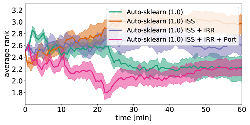
Figure 7: Ranking plot (lower is better) comparing Auto-sklearn 1.0 (1) with using only the iterative search space (2), using the iterative search space and iterative results retrieval (3) and also using a portfolio (4). Compared to Figure 6 we randomly sample $500$ combinations of the $10000$ combinations of the $10$ seeds of the $4$ AutoML systems.

B.2 Performance Without Post-Hoc Ensembling

We first give numbers comparing only Bayesian optimization, k-nearest datasets (KND) and a greedy portfolio. These results are similar to Table 2, but do not show the results of post-hoc ensembling, but using the single best model. Overall, they are qualitatively very similar, but it can be observed that the ensemble improves the average normalized balanced error rate in every case.

	10 minutes			60 minutes
	BO	KND	Port	BO	KND	Port
holdout	$7.27$	$6.43$	$\mathbf{4.76}$	$4.58$	$4.99$	$\mathbf{4.02}$
SH; holdout	$6.61$	$\underline{6.70}$	$\mathbf{5.76}$	$4.70$	$4.63$	$\mathbf{3.97}$
3CV	$9.58$	$\underline{8.95}$	$\mathbf{7.88}$	$7.10$	$\underline{7.12}$	$\mathbf{5.98}$
SH; 3CV	$8.88$	$8.97$	$\mathbf{7.20}$	$6.81$	$\underline{6.47}$	$\mathbf{6.01}$
5CV	$\mathbf{10.48}$	$\underline{15.24}$	$\underline{13.77}$	$7.34$	$7.47$	$\mathbf{5.66}$
SH; 5CV	$11.70$	$13.29$	$\mathbf{8.06}$	$7.05$	$6.69$	$\mathbf{5.93}$
10CV	$23.20$	$\underline{27.45}$	$\mathbf{18.73}$	$17.59$	$\underline{17.47}$	$\mathbf{16.17}$
SH; 10CV	$23.98$	$27.70$	$\mathbf{18.84}$	$\underline{16.94}$	$\underline{16.98}$	$\mathbf{16.07}$

Table 11: Results from Table 2 without post-hoc ensembles.

Next, we compare Auto-sklearn 2.0 with PoSH Auto-sklearn and Auto-sklearn 1.0, but again only show the performance of the single best model and not of an ensemble as in the main paper. Again, the ensemble result in uniform performance improvements with Auto-sklearn 2.0 still leading in terms of performance.

	10MIN		60MIN
	$\varnothing$	std	$\varnothing$	std
Auto-sklearn (2.0)	$\mathbf{5.01}$	$0.18$	$\mathbf{3.18}$	$0.31$
PoSH-Auto-sklearn	$5.76$	$0.12$	$3.97$	$0.22$
Auto-sklearn (1.0)	$23.24$	$0.29$	$8.68$	$0.21$

Table 12: Results from Table 5 without post-hoc ensembles.

B.3 Unaggregated results

To allow the readers to asses the performance of the individual methods on the individual datasets we present the balanced error rates before normalizing and averaging them. We give the raw results for portfolios from Table 2 in Tables 13 and 14. Additionally, we give the raw results for Auto-sklearn 2.0, PoSH Auto-sklearn and Auto-sklearn 1.0 in Tables 15 and 16.

Task ID	Name	holdout	SH; holdout	3CV	SH; 3CV	5CV	SH; 5CV	10CV	SH; 10CV
167104	Australian	$0.1721$	$0.1569$	$0.1622$	$0.1617$	$0.1583$	$0.1602$	$\mathbf{0.1556}$	$0.1559$
167184	blood-transfusion	$0.3641$	$\mathbf{0.3610}$	$0.3725$	$0.3666$	$0.3689$	$0.3722$	$0.3674$	$0.3689$
167168	vehicle	$0.2211$	$0.2267$	$0.2017$	$0.2093$	$0.2172$	$0.2052$	$0.2310$	$\mathbf{0.1870}$
167161	credit-g	$0.2942$	$\mathbf{0.2841}$	$0.2939$	$0.2955$	$0.2942$	$0.2911$	$0.2939$	$0.2934$
167185	cnae-9	$0.0658$	$0.0680$	$0.0651$	$0.0616$	$\mathbf{0.0550}$	$0.0629$	$0.0626$	$0.0553$
189905	car	$0.0049$	$0.0049$	$0.0097$	$0.0029$	$0.0047$	$0.0017$	$0.0023$	$\mathbf{0.0009}$
167152	mfeat-factors	$0.0152$	$0.0164$	$0.0141$	$\mathbf{0.0107}$	$0.0150$	$0.0117$	$0.0153$	$0.0149$
167181	kc1	$0.2735$	$0.2688$	$0.2720$	$0.2713$	$0.2547$	$0.2660$	$\mathbf{0.2477}$	$0.2719$
189906	segment	$0.0666$	$0.0687$	$0.0681$	$\mathbf{0.0620}$	$0.0664$	$0.0621$	$0.0643$	$0.0671$
189862	jasmine	$0.2044$	$0.2051$	$\mathbf{0.1982}$	$0.1986$	$0.2010$	$0.2027$	$0.2043$	$0.2027$
167149	kr-vs-kp	$\mathbf{0.0067}$	$0.0077$	$0.0093$	$0.0085$	$0.0079$	$0.0078$	$0.0071$	$0.0080$
189865	sylvine	$0.0592$	$0.0594$	$0.0600$	$0.0608$	$0.0582$	$0.0582$	$\mathbf{0.0560}$	$0.0578$
167190	phoneme	$0.1231$	$0.1245$	$0.1168$	$0.1160$	$0.1152$	$0.1136$	$\mathbf{0.1129}$	$0.1144$
189861	christine	$0.2670$	$0.2621$	$0.2608$	$0.2556$	$\mathbf{0.2517}$	$0.2567$	$0.2587$	$0.2645$
189872	fabert	$0.3387$	$0.3399$	$0.3140$	$0.3120$	$\mathbf{0.3096}$	$0.3204$	$0.3180$	$0.3172$
189871	dilbert	$0.0241$	$0.0248$	$0.0258$	$0.0220$	$\mathbf{0.0191}$	$0.0211$	$0.0303$	$0.0647$
168794	robert	$\mathbf{0.5489}$	$0.5861$	$0.5762$	$0.5583$	$0.5854$	$0.5873$	$0.6230$	$0.6230$
168797	riccardo	$0.0035$	$0.0052$	$0.0067$	$0.0054$	$\mathbf{0.0027}$	$\mathbf{0.0027}$	$0.5000$	$0.5000$
168796	guillermo	$0.2186$	$\mathbf{0.2102}$	$0.2311$	$0.2228$	$0.2165$	$0.2837$	$0.5000$	$0.5000$
75097	Amazon	$\mathbf{0.2361}$	$0.2431$	$0.2526$	$0.2526$	$0.2379$	$0.2385$	$0.2448$	$0.2443$
126026	nomao	$0.0353$	$0.0381$	$0.0360$	$0.0345$	$\mathbf{0.0312}$	$0.0331$	$0.0403$	$0.0401$
189909	jungle_chess	$0.1212$	$0.1251$	$0.1232$	$0.1156$	$0.1280$	$0.1180$	$\mathbf{0.1134}$	$0.1141$
126029	bank-marketing	$0.1397$	$0.1436$	$0.1402$	$0.1407$	$\mathbf{0.1352}$	$0.1435$	$0.1378$	$0.1362$
126025	adult	$0.1579$	$0.1575$	$0.1553$	$\mathbf{0.1540}$	$0.1591$	$0.1562$	$0.1545$	$0.1585$
75105	KDDCup09	$0.2450$	$0.2495$	$\mathbf{0.2449}$	$0.2512$	$0.2525$	$0.2487$	$0.2497$	$0.2456$
168795	shuttle	$0.0093$	$0.0086$	$0.0085$	$\mathbf{0.0084}$	$0.0085$	$0.0087$	$0.0088$	$0.0084$
168793	volkert	$0.3735$	$0.3724$	$0.3939$	$\mathbf{0.3703}$	$0.3720$	$0.3775$	$0.3867$	$0.3957$
189874	helena	$0.7483$	$0.7624$	$\mathbf{0.7475}$	$0.7478$	$0.7483$	$0.7534$	$0.7476$	$0.7575$
167201	connect-4	$0.2629$	$0.2721$	$0.2653$	$0.2630$	$\mathbf{0.2537}$	$0.2565$	$0.3003$	$0.2771$
189908	Fashion-MNIST	$\mathbf{0.1050}$	$0.1098$	$0.1217$	$0.1195$	$0.1181$	$0.1153$	$0.1437$	$0.1437$
189860	APSFailure	$0.0384$	$0.0402$	$0.0355$	$0.0364$	$0.0355$	$\mathbf{0.0354}$	$0.0410$	$0.0455$
168792	jannis	$0.3654$	$0.3685$	$0.3648$	$0.3655$	$0.3651$	$\mathbf{0.3567}$	$0.3912$	$0.3881$
167083	numerai28.6	$0.4776$	$0.4765$	$0.4752$	$0.4749$	$\mathbf{0.4747}$	$0.4775$	$0.4789$	$0.4788$
167200	higgs	$0.2736$	$0.2764$	$0.2730$	$0.2742$	$\mathbf{0.2724}$	$0.2744$	$0.2832$	$0.2844$
168798	MiniBooNE	$\mathbf{0.0581}$	$0.0589$	$0.0691$	$0.0633$	$0.0585$	$0.0644$	$0.0691$	$0.0685$
189873	dionis	$\mathbf{0.1172}$	$0.1205$	$1.0000$	$1.0000$	$1.0000$	$1.0000$	$1.0000$	$1.0000$
189866	albert	$\mathbf{0.3135}$	$0.3171$	$0.3469$	$0.3277$	$0.5000$	$0.3354$	$0.3714$	$0.3703$
75127	airlines	$0.3423$	$0.3424$	$0.3450$	$\mathbf{0.3384}$	$0.3419$	$0.3429$	$0.3408$	$0.3456$
75193	covertype	$0.0568$	$0.0564$	$0.0683$	$0.0600$	$\mathbf{0.0548}$	$0.0556$	$0.2519$	$0.2527$

Table 13: Results from Table 2 for 10 minutes using portfolios. We boldface the lowest error.

Task ID	Name	holdout	SH; holdout	3CV	SH; 3CV	5CV	SH; 5CV	10CV	SH; 10CV
167104	Australian	$0.1742$	$0.1674$	$0.1623$	$0.1626$	$0.1598$	$0.1608$	$0.1625$	$\mathbf{0.1557}$
167184	blood-transfusion	$0.3648$	$\mathbf{0.3618}$	$0.3631$	$0.3641$	$0.3689$	$0.3692$	$0.3684$	$0.3692$
167168	vehicle	$0.2125$	$0.2344$	$0.1702$	$0.1944$	$\mathbf{0.1657}$	$0.1960$	$0.1959$	$0.2151$
167161	credit-g	$0.2922$	$\mathbf{0.2895}$	$0.3035$	$0.2957$	$0.3056$	$0.2978$	$0.3008$	$0.2931$
167185	cnae-9	$0.0733$	$0.0761$	$0.0560$	$0.0616$	$0.0537$	$0.0536$	$0.0675$	$\mathbf{0.0518}$
189905	car	$0.0036$	$0.0013$	$0.0037$	$0.0098$	$\mathbf{0.0007}$	$0.0012$	$0.0008$	$0.0010$
167152	mfeat-factors	$0.0169$	$0.0186$	$0.0130$	$\mathbf{0.0117}$	$0.0139$	$0.0132$	$0.0151$	$0.0122$
167181	kc1	$0.2728$	$0.2739$	$0.2680$	$0.2724$	$0.2678$	$0.2804$	$\mathbf{0.2546}$	$0.2576$
189906	segment	$0.0708$	$0.0692$	$0.0647$	$0.0635$	$\mathbf{0.0588}$	$0.0596$	$0.0621$	$0.0613$
189862	jasmine	$0.2048$	$0.2049$	$0.1995$	$0.1989$	$0.1995$	$\mathbf{0.1976}$	$0.1995$	$0.1980$
167149	kr-vs-kp	$0.0060$	$0.0080$	$0.0081$	$0.0068$	$0.0064$	$0.0068$	$0.0055$	$\mathbf{0.0053}$
189865	sylvine	$0.0590$	$0.0591$	$0.0584$	$0.0587$	$0.0577$	$0.0578$	$\mathbf{0.0573}$	$0.0573$
167190	phoneme	$0.1222$	$0.1237$	$0.1152$	$0.1155$	$0.1111$	$0.1130$	$0.1117$	$\mathbf{0.1105}$
189861	christine	$0.2673$	$0.2666$	$0.2575$	$0.2584$	$\mathbf{0.2532}$	$0.2575$	$0.2549$	$0.2588$
189872	fabert	$0.3381$	$0.3319$	$0.3099$	$0.3097$	$0.3119$	$0.3080$	$\mathbf{0.3027}$	$0.3071$
189871	dilbert	$0.0200$	$0.0200$	$\mathbf{0.0132}$	$0.0146$	$0.0185$	$0.0209$	$0.0212$	$0.0149$
168794	robert	$0.5273$	$0.5199$	$0.5238$	$\mathbf{0.5183}$	$0.5456$	$0.5605$	$0.5652$	$0.5407$
168797	riccardo	$0.0029$	$\mathbf{0.0016}$	$0.0018$	$0.0019$	$0.0025$	$0.0076$	$0.5000$	$0.5000$
168796	guillermo	$\mathbf{0.2012}$	$0.2025$	$0.2057$	$0.2081$	$0.2100$	$0.2039$	$0.5000$	$0.5000$
75097	Amazon	$0.2376$	$0.2394$	$0.2338$	$0.2381$	$0.2431$	$0.2384$	$\mathbf{0.2312}$	$0.2324$
126026	nomao	$0.0352$	$0.0353$	$0.0334$	$0.0331$	$0.0320$	$0.0327$	$\mathbf{0.0313}$	$0.0319$
189909	jungle_chess	$0.1214$	$0.1221$	$0.1154$	$0.1172$	$0.1171$	$0.1153$	$\mathbf{0.1108}$	$0.1141$
126029	bank-marketing	$0.1388$	$0.1398$	$0.1380$	$0.1392$	$0.1382$	$0.1382$	$\mathbf{0.1370}$	$0.1380$
126025	adult	$0.1546$	$0.1541$	$0.1550$	$0.1540$	$0.1550$	$0.1550$	$0.1539$	$\mathbf{0.1538}$
75105	KDDCup09	$0.2492$	$\mathbf{0.2461}$	$0.2477$	$0.2532$	$0.2466$	$0.2488$	$0.2617$	$0.2485$
168795	shuttle	$0.0136$	$0.0107$	$0.0125$	$0.0093$	$0.0084$	$\mathbf{0.0063}$	$0.0127$	$0.0087$
168793	volkert	$0.3600$	$0.3673$	$\mathbf{0.3449}$	$0.3551$	$0.3496$	$0.3487$	$0.3581$	$0.3563$
189874	helena	$0.7449$	$0.7494$	$\mathbf{0.7331}$	$0.7369$	$0.7407$	$0.7404$	$0.7562$	$0.7452$
167201	connect-4	$0.2539$	$0.2556$	$0.2382$	$0.2428$	$0.2370$	$0.2373$	$0.2416$	$\mathbf{0.2369}$
189908	Fashion-MNIST	$0.1010$	$\mathbf{0.0971}$	$0.1046$	$0.1066$	$0.1102$	$0.1105$	$0.1191$	$0.1075$
189860	APSFailure	$0.0362$	$0.0374$	$0.0345$	$0.0364$	$0.0372$	$0.0347$	$0.0343$	$\mathbf{0.0334}$
168792	jannis	$0.3670$	$0.3638$	$0.3589$	$0.3576$	$0.3584$	$0.3565$	$\mathbf{0.3473}$	$0.3572$
167083	numerai28.6	$0.4765$	$0.4763$	$0.4774$	$0.4770$	$0.4750$	$0.4767$	$0.4755$	$\mathbf{0.4743}$
167200	higgs	$0.2712$	$0.2734$	$0.2718$	$\mathbf{0.2680}$	$0.2696$	$0.2680$	$0.2701$	$0.2683$
168798	MiniBooNE	$0.0576$	$0.0583$	$0.0560$	$\mathbf{0.0536}$	$0.0571$	$0.0565$	$0.0560$	$0.0608$
189873	dionis	$\mathbf{0.0961}$	$0.1068$	$1.0000$	$1.0000$	$1.0000$	$1.0000$	$1.0000$	$1.0000$
189866	albert	$0.3116$	$0.3168$	$0.3170$	$0.3172$	$\mathbf{0.3094}$	$0.3199$	$0.3183$	$0.3186$
75127	airlines	$0.3403$	$0.3410$	$\mathbf{0.3375}$	$0.3401$	$0.3388$	$0.3390$	$0.3398$	$0.3399$
75193	covertype	$0.0537$	$0.0519$	$0.0496$	$0.0496$	$\mathbf{0.0454}$	$0.0461$	$0.0458$	$0.0459$

Table 14: Results from Table 2 for 60 minutes using portfolios. We boldface the lowest error.

Task ID	Name	Auto-sklearn (2.0)	PoSH-Auto-sklearn	Auto-sklearn (1.0)
167104	Australian	$0.1617$	$\mathbf{0.1569}$	$0.1628$
167184	blood-transfusion	$0.3694$	$0.3610$	$\mathbf{0.3534}$
167168	vehicle	$0.2030$	$0.2267$	$\mathbf{0.1654}$
167161	credit-g	$0.2903$	$\mathbf{0.2841}$	$0.2951$
167185	cnae-9	$\mathbf{0.0635}$	$0.0680$	$0.0674$
189905	car	$\mathbf{0.0015}$	$0.0049$	$0.0057$
167152	mfeat-factors	$\mathbf{0.0123}$	$0.0164$	$0.0185$
167181	kc1	$0.2707$	$0.2688$	$\mathbf{0.2301}$
189906	segment	$0.0646$	$0.0687$	$\mathbf{0.0624}$
189862	jasmine	$0.2020$	$0.2051$	$\mathbf{0.1989}$
167149	kr-vs-kp	$0.0086$	$\mathbf{0.0077}$	$0.0089$
189865	sylvine	$0.0597$	$0.0594$	$\mathbf{0.0583}$
167190	phoneme	$\mathbf{0.1158}$	$0.1245$	$0.1257$
189861	christine	$\mathbf{0.2562}$	$0.2621$	$0.2666$
189872	fabert	$\mathbf{0.3250}$	$0.3399$	$0.3323$
189871	dilbert	$0.0240$	$0.0248$	$\mathbf{0.0066}$
168794	robert	$\mathbf{0.5861}$	$\mathbf{0.5861}$	$0.6545$
168797	riccardo	$\mathbf{0.0052}$	$\mathbf{0.0052}$	$0.5000$
168796	guillermo	$\mathbf{0.2102}$	$\mathbf{0.2102}$	$0.5000$
75097	Amazon	$0.2435$	$\mathbf{0.2431}$	$0.2610$
126026	nomao	$\mathbf{0.0336}$	$0.0381$	$0.0383$
189909	jungle_chess	$\mathbf{0.1205}$	$0.1251$	$0.1231$
126029	bank-marketing	$\mathbf{0.1402}$	$0.1436$	$0.1412$
126025	adult	$\mathbf{0.1547}$	$0.1575$	$0.1608$
75105	KDDCup09	$\mathbf{0.2460}$	$0.2495$	$0.2863$
168795	shuttle	$\mathbf{0.0084}$	$0.0086$	$0.0111$
168793	volkert	$\mathbf{0.3717}$	$0.3724$	$0.4233$
189874	helena	$\mathbf{0.7493}$	$0.7624$	$0.9157$
167201	connect-4	$\mathbf{0.2642}$	$0.2721$	$0.2809$
189908	Fashion-MNIST	$\mathbf{0.1070}$	$0.1098$	$0.1383$
189860	APSFailure	$0.0372$	$0.0402$	$\mathbf{0.0370}$
168792	jannis	$0.3654$	$0.3685$	$\mathbf{0.3637}$
167083	numerai28.6	$\mathbf{0.4753}$	$0.4765$	$0.4774$
167200	higgs	$\mathbf{0.2746}$	$0.2764$	$0.2777$
168798	MiniBooNE	$0.0603$	$\mathbf{0.0589}$	$0.0622$
189873	dionis	$\mathbf{0.1205}$	$\mathbf{0.1205}$	$0.6731$
189866	albert	$\mathbf{0.3171}$	$\mathbf{0.3171}$	$0.4407$
75127	airlines	$\mathbf{0.3404}$	$0.3424$	$0.3536$
75193	covertype	$\mathbf{0.0564}$	$\mathbf{0.0564}$	$0.8571$

Table 15: Results from Table 5 for 10 minutes. We boldface the lowest error.

Task ID	Name	Auto-sklearn (2.0)	PoSH-Auto-sklearn	Auto-sklearn (1.0)
167104	Australian	$\mathbf{0.1562}$	$0.1674$	$0.1658$
167184	blood-transfusion	$0.3669$	$0.3618$	$\mathbf{0.3572}$
167168	vehicle	$0.2187$	$0.2344$	$\mathbf{0.1822}$
167161	credit-g	$0.2980$	$\mathbf{0.2895}$	$0.3004$
167185	cnae-9	$\mathbf{0.0566}$	$0.0761$	$0.0620$
189905	car	$0.0038$	$\mathbf{0.0013}$	$0.0043$
167152	mfeat-factors	$\mathbf{0.0126}$	$0.0186$	$0.0136$
167181	kc1	$0.2600$	$0.2739$	$\mathbf{0.2250}$
189906	segment	$\mathbf{0.0609}$	$0.0692$	$0.0697$
189862	jasmine	$\mathbf{0.1971}$	$0.2049$	$0.1985$
167149	kr-vs-kp	$\mathbf{0.0060}$	$0.0080$	$0.0085$
189865	sylvine	$0.0572$	$0.0591$	$\mathbf{0.0555}$
167190	phoneme	$\mathbf{0.1140}$	$0.1237$	$0.1235$
189861	christine	$\mathbf{0.2592}$	$0.2666$	$0.2619$
189872	fabert	$\mathbf{0.3120}$	$0.3319$	$0.3185$
189871	dilbert	$0.0163$	$0.0200$	$\mathbf{0.0090}$
168794	robert	$\mathbf{0.5199}$	$\mathbf{0.5199}$	$0.5327$
168797	riccardo	$0.0016$	$0.0016$	$\mathbf{0.0016}$
168796	guillermo	$0.2025$	$0.2025$	$\mathbf{0.1964}$
75097	Amazon	$\mathbf{0.2371}$	$0.2394$	$0.2481$
126026	nomao	$\mathbf{0.0323}$	$0.0353$	$0.0361$
189909	jungle_chess	$0.1145$	$0.1221$	$\mathbf{0.1136}$
126029	bank-marketing	$\mathbf{0.1387}$	$0.1398$	$0.1428$
126025	adult	$0.1544$	$\mathbf{0.1541}$	$0.1574$
75105	KDDCup09	$0.2504$	$\mathbf{0.2461}$	$0.2549$
168795	shuttle	$\mathbf{0.0093}$	$0.0107$	$0.0109$
168793	volkert	$0.3563$	$0.3673$	$\mathbf{0.3440}$
189874	helena	$\mathbf{0.7399}$	$0.7494$	$0.7693$
167201	connect-4	$\mathbf{0.2408}$	$0.2556$	$0.2709$
189908	Fashion-MNIST	$0.1023$	$\mathbf{0.0971}$	$0.0984$
189860	APSFailure	$\mathbf{0.0343}$	$0.0374$	$0.0375$
168792	jannis	$\mathbf{0.3591}$	$0.3638$	$0.3641$
167083	numerai28.6	$\mathbf{0.4759}$	$0.4763$	$0.4760$
167200	higgs	$\mathbf{0.2690}$	$0.2734$	$0.2738$
168798	MiniBooNE	$\mathbf{0.0561}$	$0.0583$	$0.0620$
189873	dionis	$\mathbf{0.1068}$	$\mathbf{0.1068}$	$0.6731$
189866	albert	$0.3168$	$0.3168$	$\mathbf{0.3143}$
75127	airlines	$\mathbf{0.3394}$	$0.3410$	$0.3449$
75193	covertype	$\mathbf{0.0519}$	$\mathbf{0.0519}$	$0.8571$

Table 16: Results from Table 5 for 60 minutes. We boldface the lowest error.

Appendix C Theoretical properties of the greedy algorithm

C.1 Definitions

Definition 1

(Discrete derivative, from Krause and Golovin, 2014) For a set function $f:2^{\mathcal{V}}\rightarrow\mathbb{R},\mathcal{S}\subseteq\mathcal{V}$ and $e\in\mathcal{V}$ let $\Delta_{f}(e|\mathcal{S})=f(\mathcal{S}\cup\{e\})-f(\mathcal{S})$ be the discrete derivative of $f$ at $S$ with respect to $e$.

Definition 2

(Submodularity, from Krause and Golovin, 2014): A function $f:2^{\mathcal{V}}\rightarrow\mathbb{R}$ is submodular if for every $\mathcal{A}\subseteq\mathcal{B}\subseteq\mathcal{V}$ and $e\in\mathcal{V}\setminus\mathcal{B}$ it holds that $\Delta_{f}(e|\mathcal{A})\geq\Delta_{f}(e|\mathcal{B})$.

Definition 3

(Monotonicity, from Krause and Golovin, 2014): A function $f:2^{\mathcal{V}}\rightarrow\mathbb{R}$ is monotone if for every $\mathcal{A}\subseteq\mathcal{B}\subseteq V,f(\mathcal{A})\leq f(\mathcal{B})$.

C.2 Choosing on the test set

In this section we give a proof of Proposition 1 from the main paper:

Proposition 2

Minimizing the test loss of a portfolio $\mathcal{P}$ on a set of datasets $\mathcal{D}_{1},\dots,\mathcal{D}_{|\mathbf{D}_{\text{meta}}|}$, when choosing a ML pipeline from $\mathcal{P}$ for $\mathcal{D}_{d}$ based on performance on $\mathcal{D}_{d,\text{test}}$, is equivalent to the sensor placement problem for minimizing detection time (Krause et al., 2008).

Following Krause et al. (Krause et al., 2008), sensor set placement aims at maximizing a so-called penalty reduction $R(\mathcal{A})=\sum_{i\in\mathcal{I}}P(i)R(\mathcal{A},i)$, where $\mathcal{I}$ are intrusion scenarios following a probability distribution $P$ with $i$ being a specific intrusion. $\mathcal{A}\subset\mathcal{C}$ is a sensor placement, a subset of all possible locations $\mathcal{C}$ where sensors are actually placed. Penalty reduction $R$ is defined as the reduction of the penalty when choosing $\mathcal{A}$ compared to the maximum penalty possible on scenario $i$: $R(\mathcal{A},i)=\operatorname*{penalty}_{i}(\infty)-\operatorname*{penalty}_{i}(T(\mathcal{A},i))$. In the simplest case where action is taken upon intrusion detection, the penalty is equal to the detection time ($\operatorname*{penalty}_{i}(t)=t$). The detection time of a sensor placement $T(\mathcal{A},i)$ is simply defined as the minimum of the detection times of its individual members: $\min_{s\in\mathcal{A}}T(s,i)$.

In our setting, we need to do the following replacements to find that the problems are equivalent:

1. Intrusion scenarios $\mathcal{I}$: datasets $\{\mathcal{D}_{1},\dots,\mathcal{D}_{|\mathbf{D}_{\text{meta}}|}\}$,

2. Possible sensor locations $\mathcal{C}$: set of candidate ML pipelines of our algorithm $\mathcal{C}$, Detection time $T(s\in\mathcal{A},i)$ on intrusion scenario $i$: test performance $\mathcal{L}(\mathcal{M}_{C},\mathcal{D}_{d,\text{test}})$ on dataset $\mathcal{D}_{d}$,

3. Detection time of a sensor placement $T(\mathcal{A},i)$: test loss of applying portfolio $\mathcal{P}$ on dataset $\mathcal{D}_{d}$: $\min_{p\in\mathcal{P}}\mathcal{L}(p,\mathcal{D}_{d,\text{test}})$

4. Penalty function $\operatorname*{penalty}_{i}(t)$: loss function $\mathcal{L}$, in our case, the penalty is equal to the loss.

5. Penalty reduction for an intrusion scenario $R(\mathcal{A},i)$: the penalty reduction for successfully applying a portfolio $\mathcal{P}$ to dataset $d$: $R(\mathcal{P},d)=\operatorname*{penalty}_{d}(\infty)-\min_{p\in\mathcal{P}}\mathcal{L}(p,\mathcal{D}_{d,\text{test}})$.

$\blacksquare$

C.3 Choosing on the validation set

We demonstrate that choosing an ML pipeline from the portfolio via holdout (i.e. a validation set) and reporting its test performance is neither submodular nor monotone by a simple example. To simplify notation we argue in terms of performance instead of penalty reduction, which is equivalent.

Let $\mathcal{B}=\{(5,5),(7,7),(10,10)\}$ and $\mathcal{A}=\{(5,5),(7,7)\}$, where each tuple represents the validation and test performance. For $e=(8,6)$ we obtain the discrete derivatives $\Delta_{f}(e|\mathcal{A})=-1$ and $\Delta_{f}(e|B)=0$ which violates Definition 2. The fact that the discrete derivative is negative violates Definition 3 because $f(\mathcal{A})>f(\mathcal{A}\cup\{e\})$.

C.4 Successive Halving

As in the previous subsection, we use a simple example to demonstrate that selecting an algorithm via the successive halving model selection strategy is neither submodular nor monotone. To simplify notation we argue in terms of performance instead of penalty reduction, which is equivalent.

Let $\mathcal{B}=\{((5,5),(8,8)),((5,5),(6,6)),((4,4),(5,5))\}$ and $\mathcal{A}=\{((5,5),(7,7))\}$, where each tuple is a learning curve of validation-, test performance tuples. For $e=((6,5),(6,5))$, we eliminate entries 2 and 3 from $\mathcal{B}$ in the first iteration of successive halving (while we advance entries 1 and 4), and we eliminate entry 1 from $\mathcal{A}$. After the second stage, the performances are $f(\mathcal{B})=8$ and $f(\mathcal{A})=5$, and the discrete derivatives $\Delta_{f}(e|\mathcal{A})=-1$ and $\Delta_{f}(e|B)=0$ which violates Definition 2. The fact that the discrete derivative is negative violates Definition 3 because $f(\mathcal{A})>f(\mathcal{A}\cup\{e\})$.

C.5 Further equalities

In addition, our problem can also be phrased as a facility location problem (Krarup and Pruzan, 1983) and statements about the facility location problem can be applied to our problem setup as well.

Appendix D Implementation Details

D.1 Software

We implemented the AutoML systems and experiments in the Python3 programming language, using numpy (Harris et al., 2020), scipy (Virtanen et al., 2020), scikit-learn (Pedregosa et al., 2011), pandas (Wes McKinney, 2010; Reback et al., 2021), and matplotlib (Hunter, 2007). We used version 0.12.6 of the Auto-sklearn Python package for the experiments and added Auto-sklearn 2.0 functionality in version 0.12.7 which we then used for the AutoML benchmark. We give the exact version numbers used for the AutoML benchmark in Table 17.

Package	Version
Auto-sklearn 2.0	0.12.7
Auto-sklearn 1.0	0.12.6
Auto-WEKA	2.6.3
TPOT	0.11.7
H2O AutoML	3.32.1.4
Tuned Random Forest	0.24.2
AutoML benchmark	973de79617e68a881dcc640842ea1d21dfd4b36c

Table 17: Package versions used for the AutoML benchmark.

D.2 Configuration Space

We give the configuration space we use in Auto-sklearn 2.0 in Table 18.

Name	Domain	Default	Log
Classifier	(Extra Trees, Gradient Boosting, MLP,	Random Forest	-
	Passive Aggressive, Random Forest, SGD)
Extra Trees: Bootstrap	(True, False)	False	-
Extra Trees: Criterion	(gini, entropy)	gini	-
Extra Trees: Max Features	$[0.0,1.0]$	0.5	No
Extra Trees: Min Samples Leaf	$[1,20]$	1	No
Extra Trees: Min Samples Split	$[2,20]$	2	No
Gradient Boosting: Early Stopping	(off, valid, train)	off	-
Gradient Boosting: L2 Regularization	$[1e-10,1.0]$	0.0	Yes
Gradient Boosting: Learning Rate	$[0.01,1.0]$	0.1	Yes
Gradient Boosting: Max Leaf Nodes	$[3,2047]$	31	Yes
Gradient Boosting: Min Samples Leaf	$[1,200]$	20	Yes
Gradient Boosting: N Iter No Change	$[1,20]$	10	No
Gradient Boosting: Validation Fraction	$[0.01,0.4]$	0.1	No
MLP: Activation	(tanh, relu)	relu	-
MLP: Alpha	$[1e-07,0.1]$	0.0001	Yes
MLP: Early Stopping	(valid, train)	valid	-
MLP: Hidden Layer Depth	$[1,3]$	1	No
MLP: Learning Rate Init	$[0.0001,0.5]$	0.001	Yes
MLP: Num Nodes Per Layer	$[16,264]$	32	Yes
Passive Aggressive: C	$[1e-05,10.0]$	1.0	Yes
Passive Aggressive: Average	(False, True)	False	-
Passive Aggressive: Loss	(hinge, squared_hinge)	hinge	-
Passive Aggressive: Tol	$[1e-05,0.1]$	0.0001	Yes
Random Forest: Bootstrap	(True, False)	True	-
Random Forest: Criterion	(gini, entropy)	gini	-
Random Forest: Max Features	$[0.0,1.0]$	0.5	No
Random Forest: Min Samples Leaf	$[1,20]$	1	No
Random Forest: Min Samples Split	$[2,20]$	2	No
Sgd: Alpha	$[1e-07,0.1]$	0.0001	Yes
Sgd: Average	(False, True)	False	-
Sgd: Epsilon	$[1e-05,0.1]$	0.0001	Yes
Sgd: Eta0	$[1e-07,0.1]$	0.01	Yes
Sgd: L1 Ratio	$[1e-09,1.0]$	0.15	Yes
Sgd: Learning Rate	(optimal, invscaling, constant)	invscaling	-
Sgd: Loss	(hinge, log, modified Huber,	log	-
	squared hinge, perceptron)
Sgd: Penalty	(l1, l2, elasticnet)	l2	-
Sgd: Power T	$[1e-05,1.0]$	0.5	No
Sgd: Tol	$[1e-05,0.1]$	0.0001	Yes
Balancing: Strategy	(none, weighting)	none	-
Categorical Encoding: Choice	(no encoding, one hot encoding)	one hot encoding	-
Category Coalescence: Choice	(minority coalescer, no coalescense)	minority coalescer	-
Category Coalescence: Minimum Fraction	$[0.0001,0.5]$	0.01	Yes
Imputation of missing values	(mean, median, most frequent)	mean	-
Rescaling: Choice	(Min/Max, none, normalize, Power,	standardize	-
	Quantile, Robust, standardize)
Quantile Transformer: N Quantiles	$[10,2000]$	1000	No
Quantile Transformer: Output Distribution	(uniform, normal)	uniform	-
Robust Scaler: Q Max	$[0.7,0.999]$	0.75	No
Robust Scaler: Q Min	$[0.001,0.3]$	0.25	No

Table 18: Configuration space for Auto-sklearn 2.0 using only iterative models and only preprocessing to transform data into a format that can be usefully employed by the different classification algorithms. The final column (log) states whether we actually search $log_{10}(\lambda)$.

D.3 Successive Halving hyperparameters

We used the same hyperparameters for all experiments. First, we set to $eta=4$. Next, we had to choose the minimal and maximal budgets assigned to each algorithm. For the tree-based methods we chose to go from $32$ to $512$, while for the linear models (SGD and passive aggressive) we chose $64$ as the minimal budget and $1024$ as the maximal budget. Further tuning these hyperparameters would be an interesting, but an expensive way forward.

Appendix E Datasets

We give the name, OpenML task ID and the size of all datasets we used in Table 19 and 20.

name	tid	#obs	#feat	#cls
OVA_O…	75126	1545	10937	2
OVA_C…	75125	1545	10937	2
OVA_P…	75121	1545	10937	2
OVA_E…	75120	1545	10937	2
OVA_K…	75116	1545	10937	2
OVA_L…	75115	1545	10937	2
OVA_B…	75114	1545	10937	2
UMIST…	189859	575	10305	20
amazo…	189878	1500	10001	50
eatin…	189786	945	6374	7
CIFAR…	167204	60000	3073	10
GTSRB…	190156	51839	2917	43
Biore…	75156	3751	1777	2
hiva_…	166996	4229	1618	2
GTSRB…	190157	51839	1569	43
GTSRB…	190158	51839	1569	43
Inter…	168791	3279	1559	2
micro…	146597	571	1301	20
Devna…	167203	92000	1025	46
GAMET…	167085	1600	1001	2
Kuzus…	190154	270912	785	49
mnist…	75098	70000	785	10
Kuzus…	190159	70000	785	10
isole…	75169	7797	618	26
har	126030	10299	562	6
madel…	146594	2600	501	2
KDD98…	211723	82318	478	2
phili…	189864	5832	309	2
madel…	189863	3140	260	2
USPS	189858	9298	257	10
semei…	75236	1593	257	10
GTSRB…	190155	51839	257	43
India…	211720	9144	221	8
dna	167202	3186	181	3
musk	75108	6598	170	2
Speed…	146679	8378	123	2
hill-…	146592	1212	101	2
fri_c…	166866	500	101	2
MiceP…	167205	1080	82	8
meta_…	2356	45164	75	11
ozone…	75225	2534	73	2
analc…	146576	841	71	4
kdd_i…	166970	10108	69	2
optdi…	258	5620	65	10
one-h…	75154	1600	65	100
synth…	146574	600	62	6
splic…	275	3190	61	3
spamb…	273	4601	58	2
first…	75221	6118	52	6
fri_c…	75180	1000	51	2
fri_c…	166944	500	51	2
fri_c…	166951	500	51	2
Diabe…	189828	101766	50	3
oil_s…	3049	937	50	2
pol	75139	15000	49	2
tokyo…	167100	959	45	2
qsar-…	75232	1055	42	2
textu…	126031	5500	41	11
autoU…	189899	750	41	8
ailer…	75146	13750	41	2
wavef…	288	5000	41	3
cylin…	146600	540	40	2
water…	166953	527	39	2
annea…	232	898	39	5
mc1	75133	9466	39	2
pc4	75092	1458	38	2
pc3	75129	1563	38	2
porto…	211722	595212	38	2
pc2	75100	5589	37	2

name	tid	# obs	# feat	# class
satim…	2120	6430	37	6
Satel…	189844	5100	37	2
soybe…	271	683	36	19
cardi…	75217	2126	36	10
cjs	146601	2796	35	6
colle…	75212	1302	35	2
puma3…	75153	8192	33	2
Gestu…	75109	9873	33	5
kick	189870	72983	33	2
bank3…	75179	8192	33	2
wdbc	146596	569	31	2
Phish…	75215	11055	31	2
fars	189840	100968	30	8
hypot…	3044	3772	30	4
steel…	168785	1941	28	7
eye_m…	189779	10936	28	3
fri_c…	75136	1000	26	2
fri_c…	75199	1000	26	2
wall-…	75235	5456	25	4
led24…	189841	3200	25	10
colli…	189845	1000	24	30
rl	189869	31406	23	2
mushr…	254	8124	23	2
meta	166875	528	22	2
jm1	75093	10885	22	2
pc1	75159	1109	22	2
kc2	146583	522	22	2
cpu_a…	75233	8192	22	2
autoU…	75089	1000	21	2
GAMET…	167086	1600	21	2
GAMET…	167087	1600	21	2
bosto…	166905	506	21	2
GAMET…	167088	1600	21	2
GAMET…	167089	1600	21	2
churn…	167097	5000	21	2
clima…	167106	540	21	2
micro…	189875	20000	21	5
GAMET…	167090	1600	21	2
Traff…	211724	70340	21	3
ringn…	75234	7400	21	2
twono…	75187	7400	21	2
eucal…	2125	736	20	5
eleva…	75184	16599	19	2
pbcse…	166897	1945	19	2
baseb…	2123	1340	18	3
house…	75174	22784	17	2
colle…	75196	1161	17	2
BachC…	189829	5665	17	102
pendi…	262	10992	17	10
lette…	236	20000	17	26
spoke…	75178	263256	15	10
eeg-e…	75219	14980	15	2
wind	75185	6574	15	2
Japan…	126021	9961	15	9
compa…	211721	5278	14	2
vowel…	3047	990	13	11
cpu_s…	75147	8192	13	2
autoU…	189900	700	13	3
autoU…	75118	1100	13	5
dress…	146602	500	13	2
senso…	166906	576	12	2
wine-…	189836	4898	12	7
wine-…	189843	1599	12	6
Magic…	75112	19020	12	2
mv	75195	40768	11	2
parit…	167101	1124	11	2
mofn-…	167094	1324	11	2
fri_c…	75149	1000	11	2
poker…	340	829201	11	10

name	tid	#obs	#feat	#cls
fri_c…	166950	500	11	2
page-…	260	5473	11	5
ilpd	146593	583	11	2
2dpla…	75142	40768	11	2
fried…	75161	40768	11	2
rmfts…	166859	508	11	2
stock…	166915	950	10	2
tic-t…	279	958	10	2
breas…	245	699	10	2
xd6	167096	973	10	2
cmc	253	1473	10	3
profb…	146578	672	10	2
diabe…	267	768	9	2
abalo…	2121	4177	9	28
bank8…	75141	8192	9	2
elect…	336	45312	9	2
kdd_e…	166913	782	9	2
house…	75176	20640	9	2
nurse…	256	12960	9	5
kin8n…	75166	8192	9	2
yeast…	2119	1484	9	10
puma8…	75171	8192	9	2
analc…	75143	4052	8	2
ldpa	75134	164860	8	11
pm10	166872	500	8	2
no2	166932	500	8	2
LED-d…	146603	500	8	10
artif…	126028	10218	8	10
monks…	3055	554	7	2
space…	75148	3107	7	2
kr-vs…	75223	28056	7	18
monks…	3054	601	7	2
Run_o…	167103	88588	7	2
delta…	75173	9517	7	2
strik…	166882	625	7	2
mammo…	3048	11183	7	2
monks…	3053	556	7	2
kropt…	2122	28056	7	18
delta…	75163	7129	6	2
wilt	167105	4839	6	2
fri_c…	75131	1000	6	2
mozil…	126024	15545	6	2
polle…	75192	3848	6	2
socmo…	75213	1156	6	2
irish…	146575	500	6	2
fri_c…	166931	500	6	2
arsen…	166957	559	5	2
arsen…	166956	559	5	2
walki…	75250	149332	5	22
analc…	146577	797	5	6
bankn…	146586	1372	5	2
arsen…	166959	559	5	2
visua…	75210	8641	5	2
balan…	241	625	5	3
arsen…	166958	559	5	2
volca…	189902	10130	4	5
skin-…	75237	245057	4	2
tamil…	189846	45781	4	20
quake…	75157	2178	4	2
volca…	189893	8654	4	5
volca…	189890	8753	4	5
volca…	189887	9989	4	5
volca…	189884	10668	4	5
volca…	189883	10176	4	5
volca…	189882	1515	4	5
volca…	189881	1521	4	5
volca…	189880	1623	4	5
Titan…	167099	2201	4	2
volca…	189894	1183	4	5

Table 19: Characteristics of the $208$ datasets in $\mathbf{D}_{\text{meta}}$ (first part) sorted by number of features. We report for each dataset the name and the task id (as a link) as used on OpenML.org, and furthermore the number of observations, the number of features and the number of classes.

name	tid	#obs	#feat	#cls
rober…	168794	10000	7201	10
ricca…	168797	20000	4297	2
guill…	168796	20000	4297	2
dilbe…	189871	10000	2001	5
chris…	189861	5418	1637	2
cnae-…	167185	1080	857	9
faber…	189872	8237	801	7
Fashi…	189908	70000	785	10
KDDCu…	75105	50000	231	2
mfeat…	167152	2000	217	10
volke…	168793	58310	181	10
APSFa…	189860	76000	171	2
jasmi…	189862	2984	145	2
nomao…	126026	34465	119	2
alber…	189866	425240	79	2
dioni…	189873	416188	61	355
janni…	168792	83733	55	4
cover…	75193	581012	55	7
MiniB…	168798	130064	51	2
conne…	167201	67557	43	3

name	tid	#obs	#feat	#cls
kr-vs…	167149	3196	37	2
higgs…	167200	98050	29	2
helen…	189874	65196	28	100
kc1	167181	2109	22	2
numer…	167083	96320	22	2
credi…	167161	1000	21	2
sylvi…	189865	5124	21	2
segme…	189906	2310	20	7
vehic…	167168	846	19	4
bank-…	126029	45211	17	2
Austr…	167104	690	15	2
adult…	126025	48842	15	2
Amazo…	75097	32769	10	2
shutt…	168795	58000	10	7
airli…	75127	539383	8	2
car	189905	1728	7	4
jungl…	189909	44819	7	3
phone…	167190	5404	6	2
blood…	167184	748	5	2

Table 20: Characteristics of the $39$ datasets in $\mathbf{D}_{\text{test}}$ sorted by number of features. We report for each dataset the name and the task id (as a link) as used on OpenML.org, and furthermore the number of observations, the number of features and the number of classes.

References

- Alaa and van der Schaar (2018) A. Alaa and M. van der Schaar. AutoPrognosis: Automated clinical prognostic modeling via Bayesian optimization with structured kernel learning. In J. Dy and A. Krause, editors, Proceedings of the 35th International Conference on Machine Learning (ICML’18), volume 80, pages 139–148. Proceedings of Machine Learning Research, 2018.
- Balcan et al. (2021) M.-F. Balcan, T. Sandholm, and E. Vitercik. Generalization in portfolio-based algorithm selection. In Proceedings of the AAAI Conference on Artificial Intelligence (AAAI’21), volume 35, pages 12225–12232, 2021.
- Bardenet et al. (2013) R. Bardenet, M. Brendel, B. Kégl, and M. Sebag. Collaborative hyperparameter tuning. In S. Dasgupta and D. McAllester, editors, Proceedings of the 30th International Conference on Machine Learning (ICML’13), pages 199–207. Omnipress, 2013.
- Bengio and Grandvalet (2004) Y. Bengio and Y. Grandvalet. No unbiased estimator of the variance of k-fold cross-validation. Journal of Machine Learning Research, 4:1089–1105, 2004.
- Bergstra et al. (2011) J. Bergstra, R. Bardenet, Y. Bengio, and B. Kégl. Algorithms for hyper-parameter optimization. In J. Shawe-Taylor, R. Zemel, P. Bartlett, F. Pereira, and K. Weinberger, editors, Proceedings of the 24th International Conference on Advances in Neural Information Processing Systems (NeurIPS’11), pages 2546–2554. Curran Associates, 2011.
- Bergstra et al. (2013) J. Bergstra, D. Yamins, and D. Cox. Making a science of model search: Hyperparameter Optimization in hundreds of dimensions for vision architectures. In S. Dasgupta and D. McAllester, editors, Proceedings of the 30th International Conference on Machine Learning (ICML’13), pages 115–123. Omnipress, 2013.
- Biedenkapp et al. (2020) A. Biedenkapp, H. F. Bozkurt, T. Eimer, F. Hutter, and M. Lindauer. Dynamic algorithm configuration: Foundation of a new meta-algorithmic framework. In J. Lang, G. De Giacomo, B. Dilkina, and M. Milano, editors, Proceedings of the Twenty-fourth European Conference on Artificial Intelligence (ECAI’20), pages 427–434, June 2020.
- Birattari et al. (2002) M. Birattari, T. Stützle, L. Paquete, and K. Varrentrapp. A racing algorithm for configuring metaheuristics. In W. Langdon, E. Cantu-Paz, K. Mathias, R. Roy, D. Davis, R. Poli, K. Balakrishnan, V. Honavar, G. Rudolph, J. Wegener, L. Bull, M. Potter, A. Schultz, J. Miller, E. Burke, and N. Jonoska, editors, Proceedings of the Genetic and Evolutionary Computation Conference (GECCO’02), pages 11–18. Morgan Kaufmann Publishers, 2002.
- Bischl et al. (2012) B. Bischl, O. Mersmann, H. Trautmann, and C. Weihs. Resampling methods for meta-model validation with recommendations for evolutionary computation. Evolutionary Computation, 20(2):249–275, 2012.
- Bischl et al. (2021) B. Bischl, G. Casalicchio, M. Feurer, F. Hutter, M. Lang, R. Mantovani, J. van Rijn, and J. Vanschoren. OpenML benchmarking suites. In J. Vanschoren, S. Yeung, and M. Xenochristou, editors, Proceedings of the Neural Information Processing Systems Track on Datasets and Benchmarks, 2021.
- Bishop (1995) C. M. Bishop. Neural Networks for Pattern Recognition. Oxford University Press, Inc., 1995.
- Brazdil and Soares (2000) P. Brazdil and C. Soares. A comparison of ranking methods for classification algorithm selection. In R. Lopez de Mantaras and E. Plaza, editors, Machine Learning: ECML 2000, volume 1810 of Lecture Notes in Computer Science, pages 63–74. Springer, 2000.
- Brazdil et al. (1994) P. Brazdil, J. Gama, and B. Henery. Characterizing the applicability of classification algorithms using meta-level learning. In F. Bergadano and L. De Raedt, editors, Machine Learning: ECML-94, pages 83–102. Springer Berlin Heidelberg, 1994.
- Brazdil et al. (2001) P. Brazdil, C. Soares, and R. Pereira. Reducing rankings of classifiers by eliminating redundant classifiers. In P. Brazdil and A. Jorge, editors, Progress in Artificial Intelligence: Knowledge Extraction, Multi-agent Systems, Logic Programming, and Constraint Solving, Lecture Notes in Artificial Intelligence, pages 14–21. Springer, 2001.
- Brazdil et al. (2008) P. Brazdil, C. Giraud-Carrier, C. Soares, and R. Vilalta. Metalearning: Applications to Data Mining. Springer, 1 edition, 2008.
- Breimann (2001) L. Breimann. Random forests. Machine Learning Journal, 45:5–32, 2001.
- Bürger and Pauli (2015) F. Bürger and J. Pauli. A holistic classification optimization framework with feature selection, preprocessing, manifold learning and classifiers. In A. Fred, M. De Marsico, and M. Figueiredo, editors, Procceedings of 4th International Conference on Pattern Recognition: Applications and Methods (ICPRAM’15), volume 9493 of Lecture Notes in Computer Science, pages 52–68. Springer, 2015.
- Caruana et al. (2004) R. Caruana, A. Niculescu-Mizil, G. Crew, and A. Ksikes. Ensemble selection from libraries of models. In R. Greiner, editor, Proceedings of the 21st International Conference on Machine Learning (ICML’04). Omnipress, 2004.
- Caruana et al. (2006) R. Caruana, A. Munson, and A. Niculescu-Mizil. Getting the most out of ensemble selection. In Proceedings of the 6th IEEE International Conference on Data Mining (ICDM’06), pages 828–833. IEEE Computer Society Press, 2006.
- Chandrashekaran and Lane (2017) A. Chandrashekaran and I. Lane. Speeding up Hyper-parameter Optimization by Extrapolation of Learning Curves using Previous Builds. In M. Ceci, J. Hollmen, L. Todorovski, C. Vens, and S. Džeroski, editors, Machine Learning and Knowledge Discovery in Databases (ECML/PKDD’17), volume 10534 of Lecture Notes in Computer Science, pages 477–492. Springer, 2017.
- Chen et al. (2018) B. Chen, H. Wu, W. Mo, I. Chattopadhyay, and H. Lipson. Autostacker: A Compositional Evolutionary Learning System. In H. Aguirre and K. Takadama, editors, Proceedings of the Genetic and Evolutionary Computation Conference (GECCO’18), pages 402–409. ACM, 2018.
- Chen and Guestrin (2016) T. Chen and C. Guestrin. Xgboost: A scalable tree boosting system. In B. Krishnapuram, M. Shah, A. Smola, C. Aggarwal, D. Shen, and R. Rastogi, editors, Proceedings of the 22nd ACM SIGKDD International Conference on Knowledge Discovery and Data Mining (KDD’16), pages 785–794. ACM Press, 2016.
- Crammer et al. (2006) K. Crammer, O. Dekel, J. Keshet, S. Shalev-Shwartz, and Y. Singer. Online passive-aggressive algorithms. Journal of Machine Learning Research, 7(19):551–585, 2006.
- Dask Development Team (2016) Dask Development Team. Dask: Library for dynamic task scheduling, 2016. URL https://dask.org.
- de Sa et al. (2017) A. de Sa, W. Pinto, L. Oliveira, and G. Pappa. RECIPE: A grammar-based framework for automatically evolving classification pipelines. In M. Castelli, J. McDermott, and L. Sekanina, editors, EuroGP 2017: Proceedings of the 20th European Conference on Genetic Programming, volume 10196 of LNCS, pages 246–261. Springer Verlag, 2017.
- Demšar (2006) J. Demšar. Statistical comparisons of classifiers over multiple data sets. Journal of Machine Learning Research, 7:1–30, 2006.
- Domhan et al. (2015) T. Domhan, J. Springenberg, and F. Hutter. Speeding up automatic Hyperparameter Optimization of deep neural networks by extrapolation of learning curves. In Q. Yang and M. Wooldridge, editors, Proceedings of the 24th International Joint Conference on Artificial Intelligence (IJCAI’15), pages 3460–3468, 2015.
- Drori et al. (2019) I. Drori, Y. Krishnamurthy, R. Lourenco, R. Rampin, K. Cho, C. Silva, and J. Freire. Automatic machine learning by pipeline synthesis using model-based reinforcement learning and a grammar. In K. Eggensperger, M. Feurer, F. Hutter, and J. Vanschoren, editors, ICML workshop on Automated Machine Learning (AutoML workshop 2019), 2019.
- Dwork et al. (2015) C. Dwork, V. Feldman, M. Hardt, T. Pitassi, O. Reingold, and A. Roth. The reusable holdout: Preserving validity in adaptive data analysis. Science, 349(6248):636–638, 2015.
- Elsken et al. (2019) T. Elsken, J. Metzen, and F. Hutter. Neural architecture search. In Hutter et al. (2019), chapter 3, pages 63–77. Available for free at http://automl.org/book.
- Erickson et al. (2020) N. Erickson, J. Mueller, A. Shirkov, H. Zhang, P. Larroy, M. Li, and A. Smola. Autogluon-tabular: Robust and accurate automl for structured data. arXiv:2003.06505 [stat.ML], 2020.
- Escalante (2021) H. Escalante. Automated machine learning—a brief review at the end of the early years. In N. Pillay and R. Qu, editors, Automated Design of Machine Learning and Search Algorithms, pages 11–28. Springer, 2021.
- Escalante et al. (2007) H. Escalante, M. Gomez, and L. Sucar. PSMS for neural networks on the ijcnn 2007 agnostic vs prior knowledge challenge. In 2007 International Joint Conference on Neural Networks (IJCNN’07), pages 678–683. IEEE Computer Society Press, 2007.
- Escalante et al. (2009) H. Escalante, M. Montes, and E. Sucar. Particle Swarm Model Selection. Journal of Machine Learning Research, 10:405–440, 2009.
- Escalante et al. (2010) H. Escalante, M. Montes, and E. Sucar. Ensemble particle swarm model selection. In 2010 International Joint Conference on Neural Networks (IJCNN’10), pages 1–8. IEEE Computer Society Press, 2010.
- Falkner et al. (2018) S. Falkner, A. Klein, and F. Hutter. BOHB: Robust and efficient Hyperparameter Optimization at scale. In J. Dy and A. Krause, editors, Proceedings of the 35th International Conference on Machine Learning (ICML’18), volume 80, pages 1437–1446. Proceedings of Machine Learning Research, 2018.
- Feurer and Hutter (2018) M. Feurer and F. Hutter. Towards further automation in automl. In R. Garnett, F. Hutter J. Vanschoren, P. Brazdil, R. Caruana, C. Giraud-Carrier, I. Guyon, and B. Kégl, editors, ICML workshop on Automated Machine Learning (AutoML workshop 2018), 2018.
- Feurer et al. (2015a) M. Feurer, A. Klein, K. Eggensperger, J. Springenberg, M. Blum, and F. Hutter. Efficient and robust automated machine learning. In C. Cortes, N. Lawrence, D. Lee, M. Sugiyama, and R. Garnett, editors, Proceedings of the 28th International Conference on Advances in Neural Information Processing Systems (NeurIPS’15), pages 2962–2970. Curran Associates, 2015a.
- Feurer et al. (2015b) M. Feurer, J. Springenberg, and F. Hutter. Initializing Bayesian Hyperparameter Optimization via meta-learning. In B. Bonet and S. Koenig, editors, Proceedings of the Twenty-ninth National Conference on Artificial Intelligence (AAAI’15), pages 1128–1135. AAAI Press, 2015b.
- Feurer et al. (2018) M. Feurer, K. Eggensperger, S. Falkner, M. Lindauer, and F. Hutter. Practical automated machine learning for the automl challenge 2018. In R. Garnett, F. Hutter J. Vanschoren, P. Brazdil, R. Caruana, C. Giraud-Carrier, I. Guyon, and B. Kégl, editors, ICML workshop on Automated Machine Learning (AutoML workshop 2018), 2018.
- Feurer et al. (2019) M. Feurer, A. Klein, K. Eggensperger, J. Springenberg, M. Blum, and F. Hutter. Auto-sklearn: Efficient and robust automated machine learning. In Hutter et al. (2019), chapter 6, pages 113–134. Available for free at http://automl.org/book.
- Feurer et al. (2021) M. Feurer, J. van Rijn, A. Kadra, P. Gijsbers, N. Mallik, S. Ravi, A. Müller, J. Vanschoren, and F. Hutter. OpenML-Python: an extensible Python API for OpenML. Journal of Machine Learning Research, 22(100):1–5, 2021.
- Forrester et al. (2007) A. Forrester, A. Sóbester, and A. Keane. Multi-fidelity optimization via surrogate modelling. Proceedings of the royal society A: mathematical, physical and engineering sciences, 463(2088):3251–3269, 2007.
- Friedman (2001) J. Friedman. Greedy function approximation: a gradient boosting machine. Annals of statistics, 29:1189–1232, 2001.
- Fusi et al. (2018) N. Fusi, R. Sheth, and M. Elibol. Probabilistic matrix factorization for automated machine learning. In S. Bengio, H. Wallach, H. Larochelle, K. Grauman, N. Cesa-Bianchi, and R. Garnett, editors, Proceedings of the 31st International Conference on Advances in Neural Information Processing Systems (NeurIPS’18), pages 3348–3357. Curran Associates, 2018.
- Geurts et al. (2006) P. Geurts, D. Ernst, and L. Wehenkel. Extremely randomized trees. Machine Learning Journal, 63(1):3–42, 2006.
- Gijsbers et al. (2019) P. Gijsbers, E. LeDell, S. Poirier, J. Thomas, B. Bischl, and J. Vanschoren. An open source automl benchmark. In K. Eggensperger, M. Feurer, F. Hutter, and J. Vanschoren, editors, ICML workshop on Automated Machine Learning (AutoML workshop 2019), 2019.
- Gomes and Selman (2001) C. Gomes and B. Selman. Algorithm portfolios. Artificial Intelligence, 126(1-2):43–62, 2001.
- Guyon et al. (2007) I. Guyon, A. Saffari, G. Dror, and G. Cawley. Analysis of the IJCNN 2007 agnostic learning vs. prior knowledge challenge. In 2007 International Joint Conference on Neural Networks (IJCNN’07), pages 544–550. IEEE Computer Society Press, 2007.
- Guyon et al. (2010) I. Guyon, A. Saffari, G. Dror, and G. Cawley. Model selection: Beyond the Bayesian/Frequentist divide. Journal of Machine Learning Research, 11:61–87, 2010.
- Guyon et al. (2015) I. Guyon, K. Bennett, G. Cawley, H. J. Escalante, S. Escalera, Tin Kam Ho, N. Macià, B. Ray, M. Saeed, A. Statnikov, and E. Viegas. Design of the 2015 ChaLearn AutoML challenge. In 2015 International Joint Conference on Neural Networks (IJCNN’15), pages 1–8. IEEE Computer Society Press, 2015.
- Guyon et al. (2019) I. Guyon, L. Sun-Hosoya, M. Boullé, H. Escalante, S. Escalera, Z. Liu, D. Jajetic, B. Ray, M. Saeed, M. Sebag, A. Statnikov, W. Tu, and E. Viegas. Analysis of the AutoML Challenge Series 2015-2018. In Hutter et al. (2019), chapter 10, pages 177–219. Available for free at http://automl.org/book.
- H2O.ai (2020) H2O.ai. H2O: Scalable Machine Learning Platform, 2020. URL https://github.com/h2oai/h2o-3. version 3.30.0.6.
- Hall et al. (2009) M. Hall, E. Frank, G. Holmes, B. Pfahringer, P. Reutemann, and I. Witten. The WEKA data mining software: An update. SIGKDD Explorations, 11(1):10–18, 2009.
- Harris et al. (2020) C. Harris, K. Millman, S. van der Walt, R. Gommers, P. Virtanen, D. Cournapeau, E. Wieser, J. Taylor, S. Berg, N. Smith, R. Kern, M. Picus, S. Hoyer, M. van Kerkwijk, M. Brett, A. Haldane, J. del Río, M. Wiebe, P. Peterson, P. Gérard-Marchant, K. Sheppard, T. Reddy, W. Weckesser, H. Abbasi, C. Gohlke, and T. Oliphant. Array programming with numpy. Nature, 585(7825):357–362, 2020.
- Hastie et al. (2001) T. Hastie, R. Tibshirani, and J. Friedman. The Elements of Statistical Learning. Springer, 2001.
- Heffetz et al. (2020) Y. Heffetz, R. Vainshtein, G. Katz, and L. Rokach. DeepLine: AutoML Tool for Pipelines Generation using Deep Reinforcement Learning and Hierarchical Actions Filtering. In J. Tang and B. Prakash, editors, Proceedings of the 26th ACM SIGKDD International Conference on Knowledge Discovery and Data Mining (KDD’20), pages 2103–2113. ACM Press, 2020.
- Henery (1994) R. Henery. Methods for comparison. In Machine Learning, Neural and Statistical Classification, chapter 7, pages 107–124. Ellis Horwood, 1994.
- Huberman et al. (1997) B. Huberman, R. Lukose, and T. Hogg. An economic approach to hard computational problems. Science, 275:51–54, 1997.
- Hunter (2007) J. Hunter. Matplotlib: A 2d graphics environment. Computing in Science & Engineering, 9(3):90–95, 2007.
- Hutter et al. (2009) F. Hutter, H. Hoos, K. Leyton-Brown, and T. Stützle. ParamILS: An automatic algorithm configuration framework. Journal of Artificial Intelligence Research, 36:267–306, 2009.
- Hutter et al. (2011) F. Hutter, H. Hoos, and K. Leyton-Brown. Sequential model-based optimization for general algorithm configuration. In C. Coello, editor, Proceedings of the Fifth International Conference on Learning and Intelligent Optimization (LION’11), volume 6683 of Lecture Notes in Computer Science, pages 507–523. Springer, 2011.
- Hutter et al. (2019) F. Hutter, L. Kotthoff, and J. Vanschoren, editors. Automated Machine Learning: Methods, Systems, Challenges. Springer, 2019. Available for free at http://automl.org/book.
- Jamieson and Talwalkar (2016) K. Jamieson and A. Talwalkar. Non-stochastic best arm identification and Hyperparameter Optimization. In A. Gretton and C. Robert, editors, Proceedings of the Seventeenth International Conference on Artificial Intelligence and Statistics (AISTATS’16), volume 51. Proceedings of Machine Learning Research, 2016.
- Jin et al. (2019) H. Jin, Q. Song, and X. Hu. Auto-Keras: An efficient neural architecture search system. In A. Teredesai, V. Kumar, Y. Li, R. Rosales, E. Terzi, and G. Karypis, editors, Proceedings of the 25th ACM SIGKDD International Conference on Knowledge Discovery & Data Mining (KDD’19), pages 1946–1956. ACM Press, 2019.
- Kalousis and Hilario (2003) A. Kalousis and M. Hilario. Representational Issues in Meta-Learning. In T. Fawcett and N. Mishra, editors, Proceedings of the 20th International Conference on Machine Learning (ICML’03), pages 313–320. Omnipress, 2003.
- Kandasamy et al. (2017) K. Kandasamy, G. Dasarathy, J. Schneider, and B. Póczos. Multi-fidelity Bayesian Optimisation with Continuous Approximations. In D. Precup and Y. Teh, editors, Proceedings of the 34th International Conference on Machine Learning (ICML’17), volume 70, pages 1799–1808. Proceedings of Machine Learning Research, 2017.
- Karnin et al. (2013) Z. Karnin, T. Koren, and O. Somekh. Almost optimal exploration in multi-armed bandits. In S. Dasgupta and D. McAllester, editors, Proceedings of the 30th International Conference on Machine Learning (ICML’13), pages 1238–1246. Omnipress, 2013.
- Ke et al. (2017) G. Ke, Q. Meng, T. Finley, T. Wang, W. Chen, W. Ma, Q. Ye, and T.-Y. Liu. Lightgbm: A highly efficient gradient boosting decision tree. In I. Guyon, U. von Luxburg, S. Bengio, H. Wallach, R. Fergus, S. Vishwanathan, and R. Garnett, editors, Proceedings of the 30th International Conference on Advances in Neural Information Processing Systems (NeurIPS’17). Curran Associates, 2017.
- Kerschke et al. (2019) P. Kerschke, H. Hoos, F. Neumann, and H. Trautmann. Automated algorithm selection: Survey and perspectives. Evolutionary Computation, 27(1):3–45, 2019.
- Klein et al. (2017a) A. Klein, S. Falkner, S. Bartels, P. Hennig, and F. Hutter. Fast Bayesian optimization of machine learning hyperparameters on large datasets. In A. Singh and J. Zhu, editors, Proceedings of the Seventeenth International Conference on Artificial Intelligence and Statistics (AISTATS’17), volume 54. Proceedings of Machine Learning Research, 2017a.
- Klein et al. (2017b) A. Klein, S. Falkner, J. Springenberg, and F. Hutter. Learning curve prediction with Bayesian neural networks. In Proceedings of the International Conference on Learning Representations (ICLR’17), 2017b. Published online: iclr.cc.
- Kleinberg et al. (2017) R. Kleinberg, K. Leyton-Brown, and B. Lucier. Efficiency through procrastination: Approximately optimal algorithm configuration with runtime guarantees. In C. Sierra, editor, Proceedings of the 26th International Joint Conference on Artificial Intelligence (IJCAI’17), pages 2023–2031, 2017.
- Kohavi (1995) R. Kohavi. A study of cross-validation and bootstrap for accuracy estimation and model selection. In C. Mellish, editor, Proceedings of the 14th International Joint Conference on Artificial Intelligence (IJCAI’95), pages 1137–1143. Morgan Kaufmann Publishers, 1995.
- Kohavi and John (1995) R. Kohavi and G. John. Automatic Parameter Selection by Minimizing Estimated Error. In A. Prieditis and S. Russell, editors, Proceedings of the Twelfth International Conference on Machine Learning (ICML’95), pages 304–312. Morgan Kaufmann Publishers, 1995.
- Komer et al. (2014) B. Komer, J. Bergstra, and C. Eliasmith. Hyperopt-sklearn: Automatic hyperparameter configuration for scikit-learn. In F. Hutter, R. Caruana, R. Bardenet, M. Bilenko, I. Guyon, B. Kégl, and H. Larochelle, editors, ICML workshop on Automated Machine Learning (AutoML workshop 2014), 2014.
- Kotthoff (2014) L. Kotthoff. Algorithm selection for combinatorial search problems: A survey. AI Magazine, 35(3):48–60, 2014.
- Kotthoff et al. (2019) L. Kotthoff, C. Thornton, H. Hoos, F. Hutter, and K. Leyton-Brown. Auto-WEKA: automatic model selection and hyperparameter optimization in WEKA. In Hutter et al. (2019), chapter 4, pages 81–95. Available for free at http://automl.org/book.
- Krarup and Pruzan (1983) J. Krarup and P. Pruzan. The simple plant location problem: Survey and synthesis. European Journal of Operations Research, 12:36–81, 1983.
- Krause and Golovin (2014) A. Krause and D. Golovin. Submodular function maximization. In L. Bordeaux, Y. Hamadi, and P. Kohli, editors, Tractability: Practical Approaches to Hard Problems, pages 71–104. Cambridge University Press, 2014.
- Krause et al. (2008) A. Krause, J. Leskovec, C. Guestrin, J. VanBriesen, and C. Faloutsos. Efficient sensor placement optimization for securing large water distribution networks. Journal of Water Resources Planning and Management, 134:516–526, 2008.
- Kurtzer et al. (2017) G. Kurtzer, V. Sochat, and M. Bauer. Singularity: Scientific containers for mobility of compute. PloS one, 12(5), 2017.
- LeDell and Poirier (2020) E. LeDell and S. Poirier. H2O AutoML: Scalable automatic machine learning. In K. Eggensperger, M. Feurer, C. Weill, M.Lindauer, F. Hutter, and J. Vanschoren, editors, ICML workshop on Automated Machine Learning (AutoML workshop 2020), 2020.
- Leite et al. (2012) R. Leite, P. Brazdil, and J. Vanschoren. Selecting classification algorithms with active testing. In P. Perner, editor, Machine Learning and Data Mining in Pattern Recognition, volume 7376 of Lecture Notes in Computer Science, pages 117–131. Springer, 2012.
- Li et al. (2018) L. Li, K. Jamieson, G. DeSalvo, A. Rostamizadeh, and A. Talwalkar. Hyperband: A novel bandit-based approach to Hyperparameter Optimization. Journal of Machine Learning Research, 18(185):1–52, 2018.
- Lindauer et al. (2015) M. Lindauer, H. Hoos, F. Hutter, and T. Schaub. Autofolio: An automatically configured algorithm selector. Journal of Artificial Intelligence Research, 53:745–778, 2015.
- Lindauer et al. (2017) M. Lindauer, H. Hoos, K. Leyton-Brown, and T. Schaub. Automatic construction of parallel portfolios via algorithm configuration. Artificial Intelligence, 244:272–290, 2017.
- Lindauer et al. (2022) M. Lindauer, K. Eggensperger, M. Feurer, A. Biedenkapp, D. Deng, C. Benjamins, T. Ruhkopf, R. Sass, and F. Hutter. SMAC3: A versatile bayesian optimization package for Hyperparameter Optimization. Journal of Machine Learning Research (JMLR) – MLOSS, 23(54):1–9, 2022.
- Liu et al. (2020) S. Liu, P. Ram, D. Vijaykeerthy, D. Bouneffouf, G. Bramble, H. Samulowitz, D. Wang, A. Conn, and A. Gray. An ADMM based framework for automl pipeline configuration. In Proceedings of the AAAI Conference on Artificial Intelligence (AAAI’20), volume 34, pages 4892–4899, 2020.
- Malitsky et al. (2012) Y. Malitsky, A. Sabharwal, H. Samulowitz, and M. Sellmann. Parallel SAT solver selection and scheduling. In M. Milano, editor, Proceedings of the Eighteenth International Conference on Principles and Practice of Constraint Programming (CP’12), volume 7514 of Lecture Notes in Computer Science, pages 512–526. Springer, 2012.
- Mendoza et al. (2016) H. Mendoza, A. Klein, M. Feurer, J. Springenberg, and F. Hutter. Towards automatically-tuned neural networks. In F. Hutter, L. Kotthoff, and J. Vanschoren, editors, ICML workshop on Automated Machine Learning (AutoML workshop 2016), volume 64. PMLR, 2016.
- Mendoza et al. (2019) H. Mendoza, A. Klein, M. Feurer, J. Springenberg, M. Urban, M. Burkart, M. Dippel, M. Lindauer, and F. Hutter. Towards automatically-tuned deep neural networks. In Hutter et al. (2019), chapter 7, pages 135–149. Available for free at http://automl.org/book.
- Merkel (2014) D. Merkel. Docker: lightweight linux containers for consistent development and deployment. Linux journal, 2014(239), 2014.
- Metz et al. (2020) L. Metz, N. Maheswaranathan, C. Freeman, B. Poole, and J. Sohl-Dickstein. Tasks, stability, architecture, and compute: Training more effective learned optimizers, and using them to train themselves. arXiv:2009.11243[cs.LG], 2020.
- Mohr et al. (2018) F. Mohr, M. Wever, and E. Hüllermeier. ML-Plan: Automated machine learning via hierarchical planning. Machine Learning, 107(8-10):1495–1515, 2018.
- Moss et al. (2020) H. Moss, D. Leslie, and P. Rayson. MUMBO: Multi-task max-value Bayesian optimization. In F. Hutter, K. Kersting, J. Lijffijt, and I. Valera, editors, Machine Learning and Knowledge Discovery in Databases (ECML/PKDD’20), Lecture Notes in Computer Science. Springer, 2020.
- Nemhauser et al. (1978) G. Nemhauser, L. Wolsey, and M. Fisher. An analysis of approximations for maximizing submodular set functions. Mathematical Programming, 14(1):265–294, 1978.
- Niculescu-Mizil et al. (2009) A. Niculescu-Mizil, C. Perlich, G. Swirszcz, V. Sindhwani, Y. Liu, P. Melville, D. Wang, J. Xiao, J. Hu, M. Singh, W. Shang, and Y. Zhu. Winning the KDD cup orange challenge with ensemble selection. In G. Dror, M. Boullé, I. Guyon, V. Lemaire, and D. Vogel, editors, Proceedings of KDD-Cup 2009 Competition, volume 7, pages 23–34, 2009.
- Olson and Moore (2019) R. Olson and J. Moore. TPOT: A tree-based pipeline optimization tool for automating machine learning. In Hutter et al. (2019), pages 151–160. Available for free at http://automl.org/book.
- Olson et al. (2016a) R. Olson, N. Bartley, R. Urbanowicz, and J. Moore. Evaluation of a Tree-based Pipeline Optimization Tool for Automating Data Science. In T. Friedrich, editor, Proceedings of the Genetic and Evolutionary Computation Conference (GECCO’16), pages 485–492. ACM, 2016a.
- Olson et al. (2016b) R. Olson, R. Urbanowicz, P. Andrews, N. Lavender, L. Kidd, and J. Moore. Automating biomedical data science through tree-based pipeline optimization. In G. Squillero and P. Burelli, editors, Proceedings of the 19th European Conference on Applications of Evolutionary Computation (EvoApplications’16), pages 123–137. Springer, 2016b.
- Parmentier et al. (2019) L. Parmentier, O. Nicol, L. Jourdan, and M. Kessaci. TPOT-SH: A faster optimization algorithm to solve the automl problem on large datasets. In IEEE 31st International Conference on Tools with Artificial Intelligence (ICTAI’19), pages 471–478, 2019.
- Pedregosa et al. (2011) F. Pedregosa, G. Varoquaux, A. Gramfort, V. Michel, B. Thirion, O. Grisel, M. Blondel, P. Prettenhofer, R. Weiss, V. Dubourg, J. Vanderplas, A. Passos, D. Cournapeau, M. Brucher, M. Perrot, and E. Duchesnay. Scikit-learn: Machine learning in Python. Journal of Machine Learning Research, 12:2825–2830, 2011.
- Pfisterer et al. (2018) F. Pfisterer, J. van Rijn, P. Probst, A. Müller, and B. Bischl. Learning multiple defaults for machine learning algorithms. arXiv:1811.09409 [stat.ML] , 2018.
- Poloczek et al. (2017) M. Poloczek, J. Wang, and P. Frazier. Multi-Information Source Optimization. In I. Guyon, U. von Luxburg, S. Bengio, H. Wallach, R. Fergus, S. Vishwanathan, and R. Garnett, editors, Proceedings of the 30th International Conference on Advances in Neural Information Processing Systems (NeurIPS’17), pages 4288–4298. Curran Associates, 2017.
- Rakotoarison et al. (2019) H. Rakotoarison, M. Schoenauer, and M. Sebag. Automated machine learning with Monte-Carlo tree search. In S. Kraus, editor, Proceedings of the 28th International Joint Conference on Artificial Intelligence (IJCAI’19), pages 3296–3303, 2019.
- Ramage (2015) S. Ramage. Advances in meta-algorithmic software libraries for distributed automated algorithm configuration. PhD thesis, University of British Columbia, 2015. URL https://open.library.ubc.ca/collections/ubctheses/24/items/1.0167184.
- Raschka (2018) S. Raschka. Model evaluation, model selection, and algorithm selection in machine learning. arXiv:1811.12808 [stat.ML], 2018.
- Reback et al. (2021) J. Reback, jbrockmendel, W. McKinney, J. Van den Bossche, T. Augspurger, P. Cloud, S. Hawkins, gfyoung, Sinhrks, M. Roeschke, and et al. pandas-dev/pandas: Pandas 1.2.5, 2021.
- Reif et al. (2012) M. Reif, F. Shafait, and A. Dengel. Meta-learning for evolutionary parameter optimization of classifiers. Machine Learning, 87:357–380, 2012.
- Reunanen (2007) J. Reunanen. Model selection and assessment using cross-indexing. In 2007 International Joint Conference on Neural Networks (IJCNN’07), pages 2581–2585. IEEE Computer Society Press, 2007.
- Seipp et al. (2015) J. Seipp, S. Sievers, M. Helmert, and F. Hutter. Automatic configuration of sequential planning portfolios. In B. Bonet and S. Koenig, editors, Proceedings of the Twenty-ninth National Conference on Artificial Intelligence (AAAI’15). AAAI Press, 2015.
- Smith-Miles (2008) K. Smith-Miles. Cross-disciplinary perspectives on meta-learning for algorithm selection. ACM Computing Surveys, 41(1), 2008.
- Soares and Brazdil (2000) C. Soares and P. Brazdil. Zoomed ranking: Selection of classification algorithms based on relevant performance information. In D. Zighed, J. Komorowski, and J. Żytkow, editors, Principles of Data Mining and Knowledge Discovery, volume 1910 of Lecture Notes in Computer Science, pages 126–135. Springer, 2000.
- Sun et al. (2013) Q. Sun, B. Pfahringer, and M. Mayo. Towards a Framework for Designing Full Model Selection and Optimization Systems. In Multiple Classifier Systems, volume 7872, pages 259–270. Springer, 2013.
- Swersky et al. (2013) K. Swersky, J. Snoek, and R. Adams. Multi-task Bayesian optimization. In C. Burges, L. Bottou, M. Welling, Z. Ghahramani, and K. Weinberger, editors, Proceedings of the 26th International Conference on Advances in Neural Information Processing Systems (NeurIPS’13), pages 2004–2012. Curran Associates, 2013.
- Swersky et al. (2014) K. Swersky, J. Snoek, and R. Adams. Freeze-thaw Bayesian optimization. arXiv:1406.3896 [stats.ML], 2014.
- Takeno et al. (2020) S. Takeno, H. Fukuoka, Y. Tsukada, T. Koyama, M. Shiga, I. Takeuchi, and M. Karasuyama. Multi-fidelity Bayesian optimization with max-value entropy search and its parallelization. In H. Daume III and A. Singh, editors, Proceedings of the 37th International Conference on Machine Learning (ICML’20), volume 98, pages 9334–9345. Proceedings of Machine Learning Research, 2020.
- Thornton et al. (2013) C. Thornton, F. Hutter, H. Hoos, and K. Leyton-Brown. Auto-WEKA: combined selection and Hyperparameter Optimization of classification algorithms. In I. Dhillon, Y. Koren, R. Ghani, T. Senator, P. Bradley, R. Parekh, J. He, R. Grossman, and R. Uthurusamy, editors, The 19th ACM SIGKDD International Conference on Knowledge Discovery and Data Mining (KDD’13), pages 847–855. ACM Press, 2013.
- Tornede et al. (2020) A. Tornede, M. Wever, and E. Hüllermeier. Extreme algorithm selection with dyadic feature representation. In A. Appice, G. Tsoumakas, Y. Manolopoulos, and S. Matwin, editors, Discovery Science (DS), volume 12323 of Lecture Notes in Computer Science, pages 309–324. Springer, 2020.
- Tsamardinos et al. (2018) I. Tsamardinos, E. Greasidou, and G. Borboudakis. Bootstrapping the out-of-sample predictions for efficient and accurate cross-validation. Machine Learning, 107(12):1895–1922, 2018.
- Vanschoren (2019) J. Vanschoren. Meta-learning. In Hutter et al. (2019), pages 35–61. Available for free at http://automl.org/book.
- Vanschoren et al. (2014) J. Vanschoren, J. van Rijn, B. Bischl, and L. Torgo. OpenML: Networked science in machine learning. SIGKDD Explorations, 15(2):49–60, 2014.
- Vapnik (1991) V. Vapnik. Principles of risk minimization for learning theory. In J. Moody, S. Hanson, and R. Lippmann, editors, Proceedings of the 4th International Conference on Advances in Neural Information Processing Systems (NeurIPS’91). Morgan Kaufmann Publishers, 1991.
- Virtanen et al. (2020) P. Virtanen, R. Gommers, T. Oliphant, M. Haberland, T. Reddy, D. Cournapeau, E. Burovski, P. Peterson, W. Weckesser, J. Bright, S. van der Walt, M. Brett, J. Wilson, K. Millman, N. Mayorov, A. Nelson, E. Jones, R. Kern, E. Larson, C. Carey, İ. Polat, Y. Feng, E. Moore, J. VanderPlas, D. Laxalde, J. Perktold, R. Cimrman, I. Henriksen, E. Quintero, C. Harris, A. Archibald, A. Ribeiro, F. Pedregosa, P. van Mulbregt, A. Vijaykumar, Alessandro P. Bardelli, A. Rothberg, A. Hilboll, A. Kloeckner, A. Scopatz, A. Lee, A. Rokem, C. Woods, C. Fulton, C. Masson, C. Häggström, C. Fitzgerald, D. Nicholson, D. Hagen, D. Pasechnik, E. Olivetti, E Martin, E. Wieser, F. Silva, F. Lenders, F. Wilhelm, G. Young, G. Price, G.-L. Ingold, G. Allen, G. Lee, H. Audren, I. Probst, J. Dietrich, J. Silterra, J. Webber, J. Slavič, J. Nothman, J. Buchner, J. Kulick, J. Schönberger, J. de Miranda Cardoso, J. Reimer, J. Harrington, J. Rodríguez, J. Nunez-Iglesias, J. Kuczynski, K. Tritz, M. Thoma, M. Newville, M. Kümmerer, M. Bolingbroke, M. Tartre, M. Pak, N. Smith, N. Nowaczyk, N. Shebanov, O. Pavlyk, P. Brodtkorb, P. Lee, R. McGibbon, R. Feldbauer, S. Lewis, S. Tygier, S. Sievert, S. Vigna, S. Peterson, S. More, T. Pudlik, T. Oshima, T. Pingel, T. Robitaille, T. Spura, T. Jones, T. Cera, T. Leslie, T. Zito, T. Krauss, U. Upadhyay, Y. Halchenko, Y. Vázquez-Baeza, and SciPy 1.0 Contributors. SciPy 1.0: fundamental algorithms for scientific computing in Python. Nature Methods, 17(3):261–272, 2020.
- Wang et al. (2021) C. Wang, Q. Wu, M. Weimer, and E. Zhu. Flaml: A fast and lightweight automl library. In A. Smola, A. Dimakis, and I. Stoica, editors, Proceedings of Machine Learning and Systems, volume 3, pages 434–447, 2021.
- Wes McKinney (2010) Wes McKinney. Data Structures for Statistical Computing in Python. In Stéfan van der Walt and Jarrod Millman, editors, Proceedings of the 9th Python in Science Conference, pages 56 – 61, 2010.
- Winkelmolen et al. (2020) F. Winkelmolen, N. Ivkin, H. Bozkurt, and Z. Karnin. Practical and sample efficient zero-shot HPO. arXiv:2007.13382 [stat.ML], 2020.
- Wistuba et al. (2015a) M. Wistuba, N. Schilling, and L. Schmidt-Thieme. Learning Hyperparameter Optimization initializations. In Proceedings of the International Conference on Data Science and Advanced Analytics (DSAA), pages 1–10. IEEE, 2015a.
- Wistuba et al. (2015b) M. Wistuba, N. Schilling, and L. Schmidt-Thieme. Sequential Model-Free Hyperparameter Tuning. In ICDM ’15: Proceedings of the 2015 IEEE International Conference on Data Mining (ICDM), pages 1033–1038. IEEE Computer Society Press, 2015b.
- Wistuba et al. (2017) M. Wistuba, N. Schilling, and L. Schmidt-Thieme. Automatic Frankensteining: Creating Complex Ensembles Autonomously. In N. Chawla and W. Wang, editors, Proceedings of the 2017 SIAM International Conference on Data Mining (SDM’17), pages 741–749. Society for Industrial and Applied Mathematics, 2017.
- Wistuba et al. (2018) M. Wistuba, N. Schilling, and L. Schmidt-Thieme. Scalable Gaussian process-based transfer surrogates for Hyperparameter Optimization. Machine Learning, 107(1):43–78, 2018.
- Wolpert (1992) D. Wolpert. Stacked generalization. Neural Networks, 5(2):241–259, 1992.
- Wu et al. (2020) J. Wu, S. Toscano-Palmerin, P. Frazier, and A. Wilson. Practical multi-fidelity Bayesian optimization for hyperparameter tuning. In J. Peters and D. Sontag, editors, Proceedings of The 36th Uncertainty in Artificial Intelligence Conference (UAI’20), pages 788–798. PMLR, 2020.
- Xu et al. (2010) L. Xu, H. Hoos, and K. Leyton-Brown. Hydra: Automatically configuring algorithms for portfolio-based selection. In M. Fox and D. Poole, editors, Proceedings of the Twenty-fourth National Conference on Artificial Intelligence (AAAI’10), pages 210–216. AAAI Press, 2010.
- Xu et al. (2011) L. Xu, F. Hutter, H. Hoos, and K. Leyton-Brown. Hydra-MIP: Automated algorithm configuration and selection for mixed integer programming. In Proceedings of the RCRA workshop at IJCAI 2011, 2011.
- Yang et al. (2019) C. Yang, J. Akimoto, D. Kim, and M. Udell. OBOE: Collaborative filtering for AutoML model selection. In A. Teredesai, V. Kumar, Y. Li, R. Rosales, E. Terzi, and G. Karypis, editors, Proceedings of the 25th ACM SIGKDD International Conference on Knowledge Discovery & Data Mining (KDD’19), pages 1173–1183. ACM Press, 2019.
- Yang et al. (2020) C. Yang, J. Fan, Z. Wu, and M. Udell. AutoML pipeline selection: Efficiently navigating the combinatorial space. In J. Tang and B. Prakash, editors, Proceedings of the 26th ACM SIGKDD International Conference on Knowledge Discovery and Data Mining (KDD’20), pages 1446–1456. ACM Press, 2020.
- Zhang et al. (2016) Y. Zhang, M. Bahadori, H. Su, and J. Sun. FLASH: Fast Bayesian Optimization for Data Analytic Pipelines. In B. Krishnapuram, M. Shah, A. Smola, C. Aggarwal, D. Shen, and R. Rastogi, editors, Proceedings of the 22nd ACM SIGKDD International Conference on Knowledge Discovery and Data Mining (KDD’16), pages 2065–2074. ACM Press, 2016.
- Zimmer et al. (2021) L. Zimmer, M. Lindauer, and F. Hutter. Auto-Pytorch: Multi-fidelity metalearning for efficient and robust AutoDL. IEEE Transactions on Pattern Analysis and Machine Intelligence, 43(9):1–1, 2021.