True trees are dense

Abstract.

We show that any compact, connected set $K$ in the plane can be approximated by the critical points of a polynomial with two critical values. Equivalently, $K$ can be approximated in the Hausdorff metric by a true tree in the sense of Grothendieck’s dessins d’enfants.

1. Introduction

Polynomials with at most two critical values are called generalized Chebyshev polynomials or Shabat polynomials. If $p$ is such a polynomial of degree $n$ with critical values in $\{\pm 1\}$, then it is not hard to see that $T=p^{-1}([-1,1])$ is a finite planar tree with $n$ edges. We call a tree of this form a “true tree” or the “true form” of the combinatorial planar tree $T$. True trees can have all possible combinatorics, i.e., every finite planar tree has a true form and this true form is unique up to orientation preserving Euclidean similarities (see Section 2). Can true trees attain all possible “shapes”? More precisely, given a continuum (i.e., a compact, connected set) in the plane, can we find a true tree that approximates it as closely as we wish? The Hausdorff distance between two sets is the minimum $\epsilon>0$ so that each set is contained in an $\epsilon$-neighborhood of the other. In this note we prove:

Theorem 1.1.

For any compact, connected set $K\subset\mathbb{C}$ and any $\epsilon>0$ there is a polynomial $p(z)$ with critical values exactly $\pm 1$ so that $T=p^{-1}([-1,1])$ approximates $K$ to within $\epsilon$ in the Hausdorff metric. In other words, true trees are dense in all planar continua.

True trees are a special case of Grothendieck’s theory of dessins d’enfants in which a finite graph drawn on a compact topological surface $X$ induces a conformal structure on the surface and a Belyi map to the Riemann sphere (i.e., a meromorphic map branched over three points). In the case of a tree drawn on the plane, the compact surface is the Riemann sphere and the Belyi map is a polynomial with two finite critical values ($\infty$ is the third branch point). These maps have close connections to algebraic number theory and Galois theory, although we will not deal with those topics here. There is an extensive literature on dessins d’enfants, true trees and Belyi functions, e.g., see [4], [8], [11], [12], [13], [14], [17], [19], [20], [24] and their references.

Our approach to proving Theorem 1.1 is based on interpreting true trees in terms of conformal maps. We will describe this alternate formulation and reduce the theorem to a more geometric sounding statement.

Suppose $T$ is a finite tree in the plane with $n$ edges. Then the complement $\Omega$ of $T$ is the image of a conformal map $f$ from $\mathbb{D}^{*}=\{|z|>1\}$ to $\Omega$ with $f(\infty)=\infty$. We say that $T$ is “conformally balanced” if every open edge of the tree is the image under $f$ of two disjoint open arcs of length $\pi/n$ on $\partial\mathbb{D}^{*}$, and $f(z)=f(w)$ implies $f^{\prime}(z)=f^{\prime}(w)$ for almost every $z,w\in\circle{missing}.Becauseconformalmapspreserveharmonicmeasure,theconformallybalancedconditioncanberestatedintermsharmonicmeasurewithrespectto$∞$on$T$(i.e.,thefirsthittingdistributionofBrownianmotiononthespherestartedat$∞$andrununtilithits$T$).Oneachedgeofthetree,harmonicmeasurenaturallydecomposesasthesumoftwomeasures,onecorrespondingtoeachsideoftheedge.Thetreeisconformallybalancedif(1)everyedgehasthesameharmonicmeasure,and(2)whenwedecomposeharmonicmeasureoneachedgeintomeasurescorrespondingtothetwosides,thesetwomeasuresareidentical.Notethatwemeanthatthesemeasuresgivethesamemasstoeverymeasurablesubsetoftheedge,notmerelythatthewholeedgegetsequalharmonicmeasurefrombothsides.\par\par\par\par Toseethatconformallybalancedtreesareexactlythesameasthetruetreesdescribedabove,suppose$T$isaconformallybalancedtreeandlet$f$beaconformalmapfrom$D^* = {—z— ¿1}$to$Ω= C∖T$,preserving$∞$andsuchthat$1 ∈

Theorem 1.2.

For any compact, connected set $K$ and any $\epsilon>0$ there is a conformally balanced tree $T$ that is within $\epsilon$ of $K$ in the Hausdorff metric.

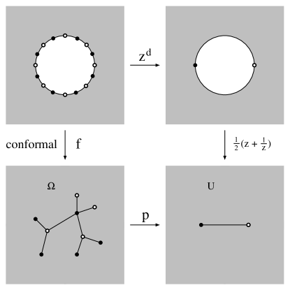
Figure 1. For any tree $T$, the composition of the conformal map from $\Omega=\mathbb{C}\setminus T$ to $\{|z|>1\}$, followed by $z^{d}$, followed by $\frac{1}{2}(z+\frac{1}{z})$ is $d$-to-$1$ and holomorphic off $T$. $T$ is conformally balanced (i.e., is a true tree) iff this map extends continuously across $T$ and hence defines a polynomial with critical values in $\{-1,1\}$.

Theorems 1.1 and 1.2 were conjectured by Alex Eremenko. I thank him for the enlightening discussion of these problems during his visit to Stony Brook in March 2011. I thank Lasse Rempe for his comments on an earlier draft of this note. I also thank the referee for a careful reading of the manuscript and numerous corrections and suggestions for improving the paper.

Kevin Pilgrim has observed that the results in this paper, combined with his arguments in [18], prove that Julia sets of post-critically finite polynomials are dense in all planar continua. The details will appear in [3]. A related result was given using different methods by Kathryn Lindsey and William Thurston in [15].

For the Shabat polynomials $p_{n}(z)=2z^{n}-1$, the only critical point is $0$, whereas the corresponding trees $T_{n}=p_{n}^{-1}([-1,1])$ become dense in the unit disk as $n$ increases. Thus it is possible for a sequence of true trees to approximate a set $K$, but the corresponding sets of critical points not to approximate $K$. However, it will be clear from our construction that the set $K$ in the theorems is approximated by both a true tree and its corresponding set of critical points (i.e., the vertices of $T$ of degreee $>1$). Moreover, the trees we construct will have a number of “bounded geomery” properties, e.g., the maximum vertex degree is $4$ and the edges are all analytic arcs with uniform estimates (i.e., each edge is the image of $I=[-1,1]$ under a map that is conformal on a uniform neighborhood $\Omega$ of $I$).

Don Marshall and Steffen Rohde have recently adapted Marshall’s conformal mapping program zipper to approximate the true form of a given planar tree, [16]. The program can handle examples with thousands of edges and is highly accurate. See Figure 2 for some examples.

         

Figure 2. Two true trees drawn by Marshall and Rohde’s program. The data on the left was a randomly constructed tree with 75 edges. The tree edges are approximated by polygons so are not highly accurate, but the vertices (i.e., the roots of the Shabat polynomials) can be computed to over a 1000 digits of accuracy. The tree on the right has 1250 edges whose combinatorics were chosen to match those of the Julia set of a certain quadratic polynomial and the resulting true tree accurately matches the shape of the Julia set.

The paper [2] contains a generalization of Theorem 1.1 from polynomials to entire functions. Given an infinite tree $T$ in the plane satisfying certain bounded geometry conditions, this paper gives a construction of an entire function with only two critical values, so that $f^{-1}([-1,1])$ approximates $T$ in a precise sense. Section 15 of [2] describes how Theorem 1.1 in this paper can be deduced from the more intricate construction in that paper. Other applications are also given, e.g., the construction of Belyi functions on certain non-compact surfaces and the existence of an entire function with bounded singular set that has a wandering Fatou component (this is impossible for entire functions with finite singular sets by a modification of Dennis Sullivan’s “non-wandering” argument for rational functions. See [5], [6], [22]).

If we require the harmonic measures for the two sides of a tree edge to be identical, but don’t require all edges to have the same harmonic measure, we get what is called a minimal continuum. These sets arise as the continua of minimal capacity that connect a given finite set. Minimal continua are studied by Herbert Stahl in [21]; this authoritative paper contains extensive history and references for the topic. I thank Alex Eremenko for pointing out the connection between balanced trees and minimal continua to me.

2. Basic properties of conformally balanced trees

In this paper, a finite plane tree $T$ will be a connected compact set in $\mathbb{C}$ that does not separate the plane and is a union of a finite collection of closed Jordan arcs, any two of which are either disjoint or have exactly one endpoint in common. The edges of the tree are the interiors of these arcs and the vertices are the endpoints. We shall say that two finite trees in the plane are equivalent if there is homeomorphism of the plane that takes one to the other. Note that this is more restrictive than saying there is a homeomorphism from one tree to the other since such a map can swap branches in a way that a planar homeomorphism cannot. See Figure 3.

Figure 3. Two planar trees that are homeomorphic but not equivalent (no homeomorphism of the plane maps one to the other).

A planar tree is locally connected, so a conformal map from $\mathbb{D}^{*}$ to $\Omega=\mathbb{C}\setminus T$, extends continuously to $\circle{missing}.Weshallalwaysassumethatsuchamapfixes$∞$.\par Let$R_n ⊂

An orientation preserving homeomorphism $\phi$ of the plane to itself is called quasiconformal (or QC for short) if it is absolutely continuous on almost all vertical and horizontal lines and satisfies $|f_{\overline{z}}|\leq k|f_{z}|$ almost everywhere for some $k<1$. Such a map is also called $K$-quasiconformal where $K=(k+1)/(k-1)$ measures the eccentricity of image ellipses of infinitesimal circles under $f$. The smallest such $K$ is called the quasiconstant of $f$. The collection of $K$-quasiconformal maps for a fixed $K$ form a compact family with respect to uniform convergence on compact sets (assuming the maps are normalized to fix $\infty$ and two finite points). See Alhfors’ book [1] for this and other properties of such maps. The function $\mu=f_{\overline{z}}/f_{z}$ is called the dilatation of the map $f$ and the size of $|\mu|$ measures how far $f$ is from conformal; if $\mu=0$ on an open set, then $f$ is conformal on that set. There is a composition law for dilatations that implies that if $f$ and $g$ have the same dilatation on an open set, then $f^{-1}\circ g$ is conformal on that set. If $f$ has zero dilatation on the whole plane, then $f$ is a conformal linear map, i.e., $f(z)=az+b$. A well known quantitative version of this fact is:

Lemma 2.1.

Given $K<\infty$ and $\epsilon>0$ there is a $\delta>0$ so the following holds. If $\psi$ is a $K$-quasiconformal map of the plane fixing $0,1,\infty$ and if its dilatation is zero except on a measure $\delta$ subset of $\mathbb{D}$, then $|f(z)-z|<\epsilon$ for every $z\in\mathbb{D}$.

Proof.

One can give more precise estimates, but this version is simply a compactness argument. If $\delta\searrow 0$, then the maps must converge on compact sets to a conformal map fixing $0,1,\infty$, i.e., the identity. ∎

The measurable Riemann mapping theorem says that given any measurable $\mu$ on the plane with $\|\mu\|_{\infty}<1$, there is a quasiconformal map $f$ with dilatation $\mu$. This is the key result about quasiconformal maps that we need, as illustrated by the following definition and lemma.

A tree $T$ is QC-balanced if there is a quasiconformal mapping $\phi:\mathbb{D}^{*}\to\Omega$ so that components of $\circle{missing}R_{2n}$ are mapped to edges of $T$ and when two components are mapped to the same edge, $\phi^{-1}\circ\phi$ is length preserving and orientation reversing between the components (this is the same the definition of conformally balanced, except that we have replaced the conformal map by a quasiconformal map).

Lemma 2.2.

Suppose $T$ is a QC-balanced tree. Then there is a quasiconformal map of the plane to itself sending $T$ to a conformally balanced tree.

Proof.

Let $\phi:\mathbb{D}^{*}\to\Omega$ be the QC map in the definition of QC-balanced and let $\mu$ be the dilatation of $\phi^{-1}$ on $\Omega$. By the measurable Riemann mapping theorem there is a quasiconformal $\psi$ on the plane with the same dilatation and thus $\psi\circ\phi$ is conformal. Hence $\psi(T)$ is conformally balanced. ∎

To say this in a slightly different way, if we compose the QC map $\phi^{-1}:\Omega\to\mathbb{D}$ with $z^{d}$ and the Joukowsky map we get a locally QC map $g$ from $\Omega$ to $U=\mathbb{C}\setminus[-1,1]$ that extends continuously to the whole plane. Then $g$ is a $d$-to-$1$ quasiregular map with singular values $\pm 1$ and the measurable Riemann mapping theorem implies there is a quasiconformal map $\phi$ so that $f=g\circ\phi^{-1}$ is a $d$-to-$1$ holomorphic map with the same singular values as $g$, i.e., $f$ is a Shabat polynomial.

Thus we can construct a conformally balanced tree by first constructing a QC-balanced tree and “fixing it” with a QC map.

Lemma 2.3.

Every finite tree in the plane can be mapped to a conformally balanced tree by a homeomorphism of the plane.

Proof.

By the previous lemma, it suffices to map $T$ to a QC-balanced tree. Every planar tree is equivalent to one with straight segments for edges and such a tree is clearly equivalent to one with smooth edges meeting with equal angles at each vertex (i.e., at a degree three vertex the edges meet at angle $120^{\circ}$). For such a tree the harmonic measures for two sides of any edge decay at the same rate at each endpoints (the decay rate may be different at the two endpoints of an edge if the endpoints have different degrees) and this means the harmonic measures for the two sides of an edge are within a bounded factor of each other (depending on the tree and the edge).

Let $E$ be the preimages of the vertices under $f$. If $T$ has $n$ edges, there are $2n$ points in $E$. The $2n$ components of $\circle{missing}E$ are paired by the relation of mapping to the same edge of $T$. Suppose $I,J$ is such a pair. Then $f^{-1}\circ f:I\to J$ defines a biLipschitz map between such a pair of corresponding arcs $I,J$. In what follows, $f^{-1}\circ f$ will always refer this this type of map (between different intervals), rather than the identity from an interval to itself.

Let $L:J\to I$ be the map that multiplies length by a factor of $|I|/|J|$ and reverses orientation. Define $L$ on $I$ to be the inverse of this map. Then $g=L\circ f^{-1}\circ f$ maps $I$ to $I$, preserves orientation and is biLipschitz. Define $g:J\to J$ to be the identity. Then define $g$ and $L$ on every other pair of edge-arcs in the same way. The result is a biLipschitz, orientation preserving map of the circle to itself so that $f(g(x))=f(L(x))$ for every $x\in\circle{missing}.Notethat$g$canbeextendedtoaquasiconformalself-map$ϕ$of$D^*$.Let$F= g(E)$.Thenthereisaquasiconformalself-map$h$of$D^*$thatmaps$E$to$R_2n$(rootsofunity)and$—h’—$isconstantoneachcomplementaryarc.\par Considerthemap$ Φ= f ∘g^-1 ∘h^-1$.Itisquasiconformalon$D^*$,maps$

Lemma 2.4.

A conformally balanced tree with $n$ edges is of the form $T=p^{-1}([-1,1])$ for some polynomial $p$ that has exactly two critical values at $\{-1,1\}$. The vertices of degree $>1$ of $T$ are exactly the critical points of $p$ and the degree equals the order of the zero of $p^{\prime}$ plus $1$. The edges of $T$ are analytic curves.

Proof.

The proof is essentially given in the introduction. The only step that was not justified there was the statement that $g(f(z)^{d}))$ “extends continuously to the whole plane and hence is entire and hence a polynomial”. This requires some proof.

We have already seen that a conformally balanced tree $T$ is the planar quasiconformal image of a finite tree with smooth edges such that all angles at vertices are non-zero. This means the complement of $T$ is a John domain and hence is removable for $W^{1,2}$ mappings (one derivative in $L^{2}$; a QC map raised to a power is in this class locally). See [9], [10]. Thus if $g(f(z)^{d})$ is a continuous function that is holomorphic off $T$, then it is entire. This finishes the proof sketched in the introduction. ∎

Lemma 2.5.

Two equivalent conformally balanced trees are the same up to a conformal linear map.

Proof.

If two conformally balanced trees have the same topology, then there is a conformal map between their complements that extends continuously to the whole plane. Since the edges of balanced tree must be analytic, they are removable for conformal maps, so the map is conformal everywhere and hence is linear. ∎

Corollary 2.6.

Every finite planar tree is equivalent to a conformally balanced tree that is unique up to linear maps.

In particular, the number of conformally balanced trees with $n$ vertices (up to linear equivalence) is the same as the number of plane trees with $n$ vertices. These can be counted using Pólya’s enumeration method as in [7], [23].

3. The construction on

The proof of Theorem 1.2 consists of constructing a tree $T$ approximating $K$, pre-composing the conformal map $f:\mathbb{D}^{*}\to\Omega=\mathbb{C}\setminus T$ by a QC self-map $\phi$ of $\mathbb{D}$ and finally post-composing $f$ by a QC map $\psi$ of $\Omega$ onto $\Omega^{\prime}=\mathbb{C}\setminus T^{\prime}$ where $T^{\prime}$ is a QC-balanced tree containing $T$ and is close to it in the Hausdorff metric. The QC map $\psi\circ f\circ\phi$ associated to $T^{\prime}$ will have uniformly bounded dilation and the support of the dilatation will have as small area as we wish, so invoking the measurable Riemann mapping theorem and Lemma 2.1 gives a conformally balanced tree that approximates $K$.

In this section we construct $T$ and the pre-composition map $\phi$ of $\mathbb{D}^{*}$. The tree $T^{\prime}$ and the QC map $\psi:\Omega\to\Omega^{\prime}$ will be constructed in the next section.

Suppose $K$ is a compact connected set. Choose a large integer $D$ and let ${\mathcal{C}}$ be the collection of dyadic square of size $2^{-D}$ that hit $K$. The corners and edges of these squares form a finite graph in the plane and we take a spanning tree for this graph. Then add segments of length $\frac{1}{4}2^{-D}$ to any vertices of degree $<4$ so that every vertex in the resulting tree $T$ has degree $1$ or $4$, every edge is still vertical or horizontal and every edge has length either $2^{-D}$ or $2^{-D-2}$. See Figure 4. The tree $T$ approximates $K$ to within $2^{-D+1}$ in the Hausdorff metric.

Figure 4. A continua is covered by dyadic boxes and an approximated tree is formed from the boxes’ edges. Some extra segments are added to make every degree $1$ or $4$ and every edge have length $2^{-D}$ or $2^{-D-2}$.

Why did we add the extra segments to make every degree $1$ or $4$? This is more of a convenience than a necessity. The condition insures that for any edge, the harmonic measures for the two sides have the same behavior as we approach an endpoint, i.e., $\frac{d\omega_{1}}{d\omega_{2}}$ is bounded above and below on the whole edge (in fact, this function extends to be analytic on a neighborhood of the edge). The precise version of this fact that we will use is:

Lemma 3.1.

Suppose $e$ is an open edge of $T$, $f:\mathbb{D}^{*}\to\Omega$ is a conformal map onto the exterior of $T$ and $I,J\subset\circle{missing}arethetwocomponentsof$f^-1(e)$.Themap$ g=f^-1 ∘f$definedfrom$I$to$J$hasanextensiontoaconformalmapfromaneighborhood$Ω_I$of$I$toaneighborhood$Ω_J$of$J$.Moreover,$${\rm{dist}}(I,\partial\Omega_{I})\geq C_{1}|I|,$$forsomeabsolute$ C_1 ¿0$.Thesameestimateholdsfor$J$and$Ω_J$.Also,$$C_{2}^{-1}\leq|g^{\prime}|\frac{|I|}{|J|}\leq C_{2}$$on$I$forsomeabsolute$C_2 ¡ ∞.

Proof.

This is just an application of the Schwarz reflection principle. We first consider the case when the endpoints of $e$ both have degree $4$, as in Figure 5. Let $e^{\prime}$ be the edge $e$ with perpendicular segments of length $\frac{1}{4}|e|$ added at either end, so as to bound three sides of a rectangle $R$, whose preimage under $f$ is an open set $\Omega_{I}^{+}$ in $\mathbb{D}^{*}$ with $I$ in its boundary. This open set, together with its boundary $I^{\prime}$ on $\circle{missing}anditsreflectionacross$

Map $\Omega_{I}^{+}$ to $R$ by $f$, follow by a reflection across $e$ to another rectangle, map this to a set $\Omega_{J}^{+}$ by $f^{-1}$ and reflect this across $\circle{missing}totheset$Ω_J^-$.Let$Ω_J$betheunionof$Ω_J^+, Ω_J^-$andtheinterior(in$

This composition is made up of two conformal maps and two reflections, so is a conformal map $\Omega_{I}^{+}\to\Omega_{J}^{-}$ and sends $I^{\prime}$ to $J^{\prime}$, so by the Schwarz reflection principle, it extends to be a conformal map from $\Omega_{I}$ to $\Omega_{J}$.

Clearly the harmonic measure of $e$ in $\Omega=\mathbb{C}\setminus T$ from any point of the opposite side of $R$ is bounded uniformly away from one, so the same is true of $I$ in $\mathbb{D}^{*}$ from any point of $\partial\Omega_{I}\cap\mathbb{D}^{*}$. This implies $\partial\Omega_{I}$ is at least distance $C_{1}|I|$ from $I$ for some absolute $C_{1}$. The same applies to $J$ and $\Omega_{J}$. The Koebe $\frac{1}{4}$-theorem now implies that $g$ has derivative comparable to $|J|/|I|$ on $I$, again with absolute constants.

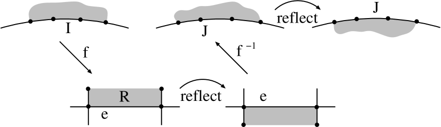
Figure 5. Proof that $g=f^{-1}\circ f$ has a conformal extension to a neighborhood of $I$ if the image connects two vertices of degree $4$.

If $e$ has one vertex of degree $1$ and the other of degree $4$, the argument is very similar. In this case, the intervals $I$ and $J$ are adjacent and we take $R$ as shown in Figure 6. Its preimage under $f$ is the light gray region above the circle that we will denote $\Omega_{IJ}^{+}$, and the darker region below the circle is its reflection $\Omega_{IJ}^{-}$. As before, the composition of the four maps is conformal between these domains, and hence it has a conformal extension from the obvious domain $\Omega_{IJ}$ to itself. The remaining conclusions follow just as before.

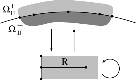
Figure 6. Proof that $g=f^{-1}\circ f$ has a conformal extension to a neighborhood of $I$ if the image connects a degree $1$ and degree $4$ vertex.

∎

So the restriction of the mapping $g=f^{-1}\circ f$ to any component of $\circle{missing}E$ has a conformal extension to a uniformly larger neighborhood (recall $E$ are the preimages under $f$ of the vertices of $T$), although the map itself may have jump discontinuities at the points of $E$. This is not quite the same as “piecewise analytic” since this term usually includes continuity at the endpoints. We want to approximate $g$ by a piecewise linear map on each component of $\circle{missing}E$ by adding more points into the gaps between $E$ and linearly interpolating the values of $g$ between these points.

Lemma 3.2.

Suppose $g$ is as above. Then there is a quasiconformal map $\phi$ of $\mathbb{D}^{*}$ to itself, and a finite set $F\subset\circle{missing}sothat$ϕ(F)$contains$E$andsothat$ ϕ^-1∘g ∘ϕ$ispiecewiselinearoneachcomponentof$

Proof.

Consider a pair $I,J$ of components of $\circle{missing}E$ that map to the same edge of $T$. Subdivide $I$ and on each subinterval, let $\phi$ be defined as $g$ followed by the linear map from $J=g(I)$ back to $I$ that inverts $g$ at the endpoints. On the interval $J=g(I)$, $\phi$ is defined to be the identity. Since $g$ is smooth, $\phi$ is biLipschitz with constant as close to $1$ as we want if the subdivision of $I$ is fine enough. We can therefore extend it to a quasiconformal map of the Carleson region

$$Q_{I}=\{z\in\mathbb{D}^{*}:z/|z|\in I,|z|-1<|I|\},$$

to itself that is the identity on $\partial Q_{I}\setminus I$. Define $\phi$ on the rest of $\mathbb{D}^{*}$ as the identity and define it in $\mathbb{D}$ by reflection. This map has the desired piecewise linear property, but we still need to adjust the sizes of the intervals.

To make adjacent intervals have comparable length with a factor of $2$, we simply split the larger in 2 equal pieces whenever this fails; the shortest interval will never be split and a shorter interval will never be produced, so the process ends after a finite number of steps.

To make notation easier, we normalize arclength on the circle to be $1$. To make sure that the normalized interval lengths are powers of $2$, cover the circle by disjoint dyadic intervals that are at most $1/4$ as long as any of the intervals from the collection that they hit, and that are maximal with respect to this property. Such a dyadic interval has at least $\frac{1}{8}$th of the length of the shortest interval it hits, and is contained in the union of this interval and one of its neighbors, which is at most twice as long. Thus each of our dyadic intervals has length between $\frac{1}{4}$ and $\frac{1}{16}$ times the length of any interval in our collection that it intersects.

If we replace each interval $I$ in ${\mathcal{I}}$ by the union of dyadic intervals in ${\mathcal{D}}$ that are contained in $I$ or contain $I$’s left endpoint, the new interval $I^{\prime}$ has comparable length and is a union of between $4$ and $16$ dyadic intervals. By splitting some of the dyadic intervals in two, we can insure it is always a union of $16$ dyadic intervals.

If necessary, we can repeat the “split the larger neighbor” argument to insure adjacent intervals have lengths within a factor of $2$ of each other. We end by splitting every interval into four equal subintervals to make sure every interval has at least one equal sized neighbor. If $I$ and $J$ are both adjacent to a point mapping to a vertex, but are not of equal length, then one is exactly twice as long as the other. Subdivide the longer one and the adjacent interval of the same length. Then the two segments adjacent to the vertex preimage are equal and all the intervals still satisfy all the other requirements. This final collection is the desired collection ${\mathcal{I}}$. ∎

4. The construction on $T$

In this section, we define a tree $T^{\prime}$ containing $T$ and a series of quasiconformal maps

$$\mathbb{C}\setminus T=\Omega\to\Omega_{0}\to\Omega_{1}\to\Omega_{2}\to\Omega_{3}\to\Omega_{4}=\mathbb{C}\setminus T^{\prime}.$$

If we denote the composition by $\psi$, then our construction will have the property that $T^{\prime}$ is a QC-balanced tree via the map $\psi\circ f\circ\phi:\mathbb{D}^{*}\to\mathbb{C}\setminus T^{\prime}$. Moreover, the dilatation of this map will be uniformly bounded and the support of its dilation is mapped into as small a neighborhood of $T$ as we wish (equivalently, the inverse map, which automatically has the same quasiconstant, has dilatation supported in an arbitrarily small neighborhood of $T$). Thus using Lemmas 2.1 and 2.2 will yield a conformally balanced tree that approximates $T$, and hence $K$.

To simplify, we will rescale $T$ to correspond to a unit grid (i.e., take $D=0$).

In order to draw simpler pictures, we want to avoid the corners in $T$ created by the vertices of degree $4$. The first map $\psi_{0}:\Omega\to\Omega_{0}\subset\Omega$ simply pulls the domain way from these corners in a uniformly QC way. Choose $0<\delta\ll 1$ to be a small power of $2$ (how small will be determined during the course of the construction) and for each degree $4$ vertex in $T$ remove the four $\delta\times\delta$ subsquares of $\Omega$ that have this vertex as a corner. This gives $\Omega_{0}$. Let $\Omega^{\prime}$ be $\Omega$ with slits of length $\sqrt{2}\delta$ bisecting each corner of $\Omega$ removed (these are diagonals of the squares we just removed). There is a uniformly quasiconformal map $\psi_{0}:\Omega^{\prime}\to\Omega_{0}$ that is affine on each edge and equals the identity outside a $\delta$-neighborhood of $T$. See Figure 7. (Note that $\psi_{0}$ is not quasiconformal on $\Omega$ because it is not continuous along the slits defining $\Omega^{\prime}$, but we will finish the construction by composing with $\psi_{0}^{-1}$ to “fill in” the corners and the composed map will have a continuous, quasiconformal extension to all of $\Omega$.)

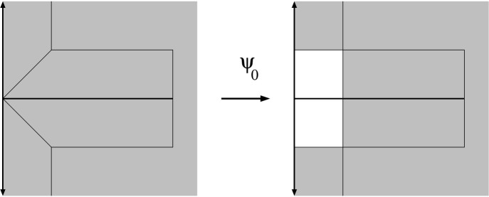
Figure 7. The map $\psi_{0}:\Omega\to\Omega_{0}$. It pulls the domain away from the corners.

Now we define $\Omega_{1}$ as the set of points $z\in\Omega_{0}$ such that

$${\rm{dist}}(z,T)>\delta\quad\text{ or }\quad{\rm{dist}}(z,T)>\sqrt{2}{\rm{dist}}(z,V_{1}),$$

where $V_{1}$ is the finite set of degree $1$ vertices of $T$. Thus $\Omega_{1}$ is a polygon where most of the edges are parallel to edges of $T$, except in a neighborhood of each degree one vertex where the boundary slopes down to hit $T$ at the vertex. We can clearly map $\Omega_{0}\to\Omega_{1}$ by a uniformly QC map with dilatation supported in a $\delta$-neighborhood of $T$. See Figure 8. If $\delta$ is small enough then any interval of length $\delta$ with one endpoint at a degree $1$ vertex of $T$ is contained in the image of the two ${\mathcal{I}}$ intervals on the circle that are adjacent to that vertex. Assume $\delta$ has been chosen small enough to make this happen at every degree $1$ vertex.

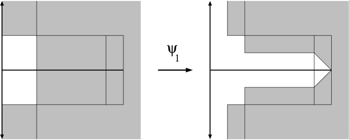
Figure 8. The map $\psi_{1}:\Omega_{0}\to\Omega_{1}$.

Let ${\mathcal{J}}$ denote the segments in $T$ that are of the form $\partial\Omega_{0}\cap e$ for some edge $e$ of $T$. Each edge $e$ of $T$ either connects two vertices of degree four or connects a vertex of degree four to a vertex of degree one. In the first case, segments in ${\mathcal{J}}$ consist of $e$ with two intervals of length $\delta$ removed (one at each endpoint), and in the second case we only remove an interval at the degree four vertex.

The map $\psi_{0}\circ f\circ\phi^{-1}$ sends each element of ${\mathcal{I}}$ into some element of ${\mathcal{J}}$. Since each element of ${\mathcal{I}}$ has measure that is a power of $2$, there is a smallest and largest power that occur and we denote these by $2^{-n}$ and $2^{N-n}$. Then the measure of each element that occurs can be written as $2^{m}2^{-n-N}$ where $N\leq m\leq 2N$. By taking $N$ larger, if necessary, we can assume $2^{-n-N}$ evenly divides $1-2\delta$ and $\frac{1}{4}-\delta$ (the two possible lengths of edges in ${\mathcal{J}}$). Thus each element of ${\mathcal{J}}$ can be divided into an integer number of disjoint sub-segments of length $2^{-n-N}$. This collection of subintervals is called ${\mathcal{K}}$. Taking $N$ larger, if necessary, we may assume $2N2^{-n-N}<\delta$.

Each element $K\in{\mathcal{K}}$ is associated to two elements of ${\mathcal{I}}$ whose images contain $K$ and that correspond to the two sides of $K$. If the measure of one of these intervals is $2^{m}2^{-n-N}$ we call $m$ one of the two “heights” associated to $K$. Each height is associated to one side of $K$. Lemma 3.2 implies that the heights of intervals in $K$ do not change very quickly. In fact, that lemma implies the following facts about intervals in ${\mathcal{K}}$:

1. adjacent intervals have heights differing by at most $1$,

2. every interval has the same height as at least one of its neighboring intervals,

3. given a degree $1$ vertex $v$ of $T$, every interval within distance $\delta$ of $v$ has the same height,

4. given one of the $\delta\times\delta$ squares removed from $\Omega$ to form $\Omega_{0}$, the two intervals adjacent to that square have the same height. They also have the same heights as the neighboring intervals that are not adjacent to the removed square.

Next we build $\Omega_{2}$. For each segment $K\in{\mathcal{K}}$ in $\partial\Omega_{0}$ we add a rectangle or trapezoid to both sides as follows. First suppose $K=[a,b]$ is within distance $\delta$ of a degree $1$ vertex $v$. This means that the heights of $K$ for either side are the same by Lemma 3.2 if $\delta$ has been chosen small enough (since intervals adjacent to a vertex of the tree have equal measure). If $m$ denotes the height associated to $K$, and if

$$m|K|\geq{\rm{dist}}(K,v_{1})+|K|.$$

then we add a rectangle of size $|K|\times m|K|$ to both sides of $K$. Otherwise we add a trapezoid with one side $K$, two sides perpendicular to $K$ and the fourth side on $\partial\Omega_{1}$. See Figure 9.

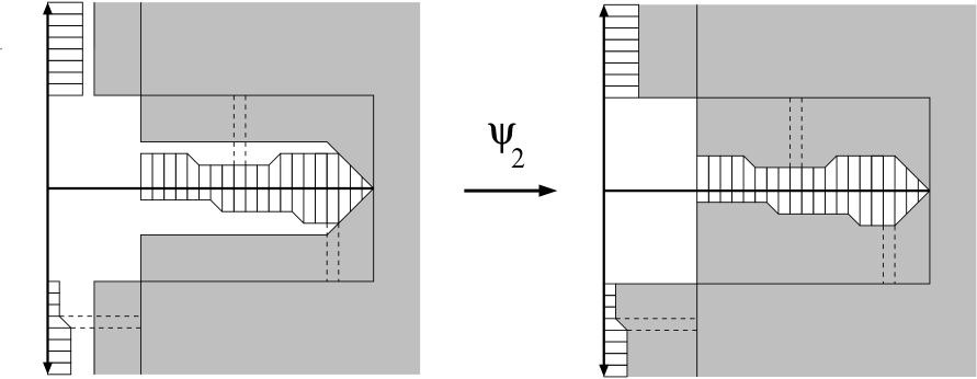
Figure 9. We map $\psi_{2}:\Omega_{1}\to\Omega_{2}$ by pushing the boundary back towards $T$. The map is the identity for points more than $\delta$ from $T$.

If $K$ is more than distance $\delta$ from any degree one vertex then consider one side of $K$ and the two adjacent intervals. If all three intervals have the same height $m$, then we add a $|K|\times m|K|$ rectangle with $K$ as one side. Otherwise, one of the adjacent intervals has the same height $m$ as $K$ and the other has height $m^{*}$ differing by $1$. We add a trapezoid with base $K$, and two parallel sides that are perpendicular to $K$ with side lengths $m|K|$ and $m^{*}|K|$. The fourth side of the trapezoid is opposite $K$ and has length $\sqrt{2}|K|$.

If $K$ has only one neighbor, it must be adjacent to one of the removed “corner squares” of $\Omega_{0}$. As noted earlier, it must have the same height as its immediate neighbor, as well as the other interval of ${\mathcal{K}}$ adjacent to the same corner square.

Let $W$ be the union of all these closed rectangles and trapezoids, together with the closures of $\delta\times\delta$ squares removed from $\Omega$ to form $\Omega_{0}$. The union is a closed connected set and the complement is the open set $\Omega_{2}$. Clearly $\Omega_{1}$ can be mapped to $\Omega_{2}$ by a quasiconformal map $\psi_{2}$ that is piecewise affine, has uniformly bounded quasiconstant and has dilatation supported in a $\delta$-neighborhood of $T$. See Figure 9.

If we add all the open rectangles and trapezoids to $\Omega_{1}$, along with their edge on $\partial\Omega_{2}$, we get an open set $\Omega_{3}$ containing $\Omega_{2}$. We define $\Omega_{4}=\psi_{0}^{-1}(\Omega_{3})$ and $T^{\prime}=\partial\Omega_{r}$. Clearly this is a linear tree that contains $T$. See Figure 10.

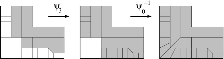
Figure 10. The map $\psi_{3}:\Omega_{2}\to\Omega_{3}$ fills in rectangles and trapezoids and then $\psi_{0}^{-1}$ “refills” the corners. The composition $\psi=\psi_{0}^{-1}\circ\psi_{3}\circ\psi_{2}\circ\psi_{1}\circ\psi_{0}$ has uniformly bounded dilatation, is the identity outside a $\delta$-neighborhood of $T$ and has a continuous extension $\Omega\to\Omega_{4}$.

The only object not yet defined is the quasiconformal map $\psi_{3}:\Omega_{2}\to\Omega_{3}$. Again, the map is the identity far from $T$, and each connected component of $\Omega_{3}\setminus\Omega_{2}$ is a rectangle or a trapezoid (we will denote either type of region by $R$) and is the image under $\psi_{3}$ of a square in $\Omega_{2}$ that shares a side with $R$. See Figure 11. There are three types of maps to describe: $m$-rectangle maps, $m$-trapezoid maps and $m$-tip maps. Each of these maps takes a region in $\Omega_{2}$ (either a triangle or square) with one boundary segment $I$ on $\partial\Omega_{2}$ and expands it into the component of $\Omega_{3}\setminus\Omega_{2}$ attached along $I$ (this component is either a rectangle, a trapezoid or a triangle). See Figure 11. Each map is the identity on $\partial R\cap\Omega_{2}$, so the map can be extended as the identity to the rest of the plane. We will describe each type of map separately.

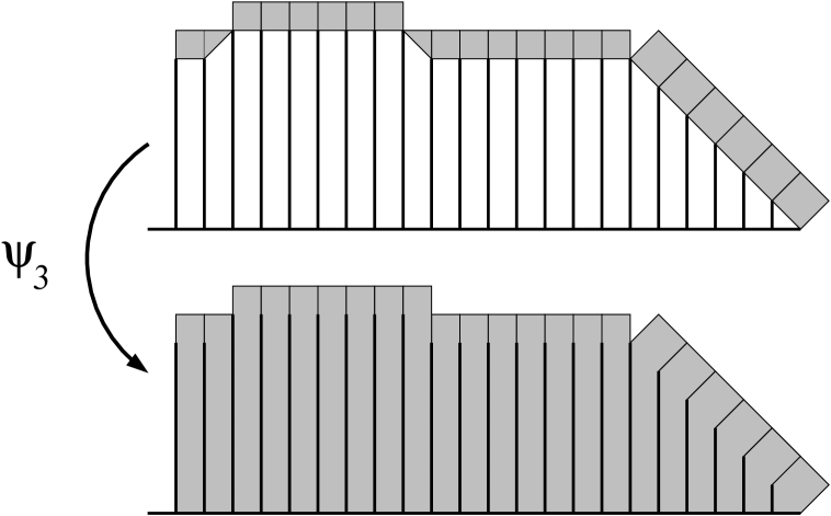
Figure 11. The map $\psi_{3}:\Omega_{2}\to\Omega_{3}$ is made up of three types of maps that expand a square or triangle in $\Omega_{2}$ into a rectangle or trapezoid in $\Omega_{3}\setminus\Omega_{2}$.

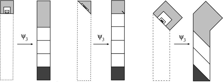
Figure 12. This shows in more detail how the map in Figure 11 expands $\Omega_{2}$ into $\Omega_{3}$. In each case the domain is cut into decreasing, nested pieces and the pieces are expanded to shapes that fill the image. The boundary expansion on the $k$th piece is $2^{k}$ in a sense that is made precise in the text. The details of each type of map are shown in Figures 13, 14 and 15.

Rectangle maps: An $m$-rectangle map sends a unit square $S$ to a $1\times m$ rectangle $R$. We write $R$ as a union of $m$ adjacent unit squares $R=\cup_{k=1^{m}}S_{k}$ with $S_{1}=S$. The boundary values of the map are as follows. The map is the identity on $\partial S\cap\partial R$ (this is three sides of the square) and the fourth side is mapped to the rest of $R$. starting at the endpoints, divide the fourth side symmetrically into two intervals of lengths $4^{-k}$ for $k=1,\dots,m$ (the longest adjacent to the endpoints, the shortest adjacent to the midpoint). For $k=1,\dots m$ intervals of length $4^{-k}$ are mapped affinely to the part of $\partial S_{k}$ on the long sides of $R$. The union of the two intervals of length $2^{-m}$ is mapped affinely to the short side of $R$ on $\partial S_{k}$. That these boundary values can be attained by a uniformly quasiconformal map is apparent from the diagrams in Figures 12 and 13.

The first figure shows how to subdivide the square into $m-1$ nested polygonal regions $P_{1},\dots,P_{m-1}$; $P_{1}$ maps to a $1\times 2$ sub-rectangle in $R$, $P_{2},\dots,P_{m-2}$ are all similar to each other and map to squares, and $P_{m-1}$ is a square mapping to a square (but not in the obvious way, since one of its sides must map to three sides in the image). These three maps are constructed in Figure 13 by showing compatible triangulations for domains and ranges (i.e., the triangulations are in a 1-1 correspondence that preserves adjacency). Given compatible triangulations of two regions we can define a quasiconformal map between them by taking the obvious piecewise affine maps between triangles. It is now an easy exercise to check that the mappings induced by the triangulations have the boundary values described above.

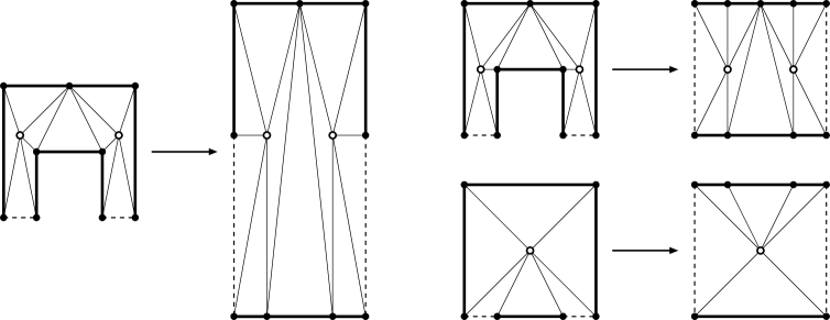
Figure 13. The $m$-rectangle map sends a square to a $1\times m$ rectangle. The map is composed from three types of pieces: one each for mapping onto the “top” box (lighter shading in Figure 12) and “bottom” (darker) and another that is repeated in all the “middle” boxes (white). The triangulations define piecewise affine maps between the polygons.

Trapezoid maps: A $m$-trapezoid map also maps into a $1\times m$ rectangle $R$ as above, but the domain of this map is now a right triangle that we may identify with one half of the top square cut by a diagonal. The boundary map is the identity on the legs of this triangle. There is an asymmetry to the construction and we assume the picture is as shown in Figure 12, so that the domain of the map is the upper right half of the top square. The hypotenuse of the triangle is divided into pairs of intervals of size $4^{-k}$, $k=1,\dots$ as before and the left half is mapped to the left side of the rectangle as before. On the right side the rightmost interval has length $\frac{1}{4}$ and is folded onto itself to form a slit of length $1/8$ in the rectangle; this slit is not in the image of the interior. The remaining smaller intervals are mapped to the right side of the rectangle just as before. Figure 14 shows how to divide the triangle into regions and map these regions into the rectangle. We only show the details for the top piece; the lower pieces are affinely stretched to be similar to the rectangle map pieces and then mapped exactly as in the rectangle maps.

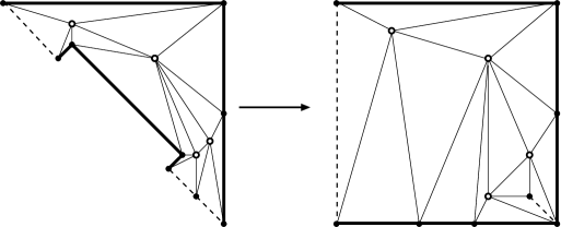
Figure 14. The $m$-trapezoid map sends the triangle to a $1\times m$ rectangle. The middle and bottom maps are the same, after an affine stretching, to the middle and bottom maps of the rectangle map, so we only show the construction for the top piece. Note that the image is not a simple polygon; a piece of the boundary is folded onto itself to form a slit in the image. This is necessary for the trapezoid map to match rectangle maps of different heights on either side.

Note that $m$-trapezoid maps interpolate between $m$-rectangle maps and $(m-1)$-rectangle maps. The boundary segments of $\partial\Omega_{2}$ corresponding to each map have measure $2^{m}2^{-n-M}$. Dividing these segments into $2^{m+1}$ equal, disjoint subsegments and applying the “filling map” partitions the sides and bottom of the rectangular image into intervals. Whenever two rectangles or trapezoids share a side, we want the partitions of these sides to be identical. Each piece of the partition is one edge of our QC-balanced tree and we want them to have equal measure. Obviously two rectangles maps of the same height match up and the definition of the $m$-trapezoid map is designed so that it matches a $m$-rectangle map on one side and a $(m-1$)-rectangle map on the other. The top side of an $(m-1)$-rectangle map has half the measure of the top of a $m$-rectangle, so the trapezoid map matches up intervals of equal measure.

Tip maps: The third type of map is the $m$-tip map. The details are described in Figure 15. Each $m$-tip map is designed to match a $(m+1)$-tip map (or a $m$-rectangle map) on its longer vertical side and a $(m-1)$-tip map on its shorter vertical side. Once again the boundary map is the identity on the top three sides of the domain, and maps the bottom side to the sides and bottom of the image trapezoid. The bottom side of the domain square is again divided into symmetric pairs of intervals of length $4^{-m}$. The leftmost and rightmost are mapped to the unit segments of the trapezoids vertical sides, but since these sides are different lengths, the images are displaced vertically with respect to each other, so they form the vertical sides of a parallelogram. Intervals of length $4^{-k}$ are mapped to vertical sides of the lower parallelograms. After $m$ steps, the parallelogram hits the bottom edge and the rest of the domain square is mapped to the bottom triangle as illustrated in Figure 15. The last map, adjacent to the tip, is a special case that is illustrated in Figure 15.

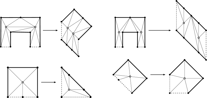
Figure 15. The $m$ tip maps also fills in a trapezoid, but is different from a trapezoid map because it has to match other tip maps, not two rectangle maps of different heights. Again, it is built from three types of map: top, bottom and middle. Along its left side (for the orientation shown) it matches a $m$-rectangle map or the right side of a $(m+1)$-tip map and on the right it matches the right side of a $(m-1)$-tip map. The $1$-tip map requires a special construction, as shown at lower right.

All the top intervals of the tip trapezoids have the same measure, so the tip maps match intervals of the same measure along the vertical sides. Tip maps for opposite sides of an interval $K\in{\mathcal{K}}$ are the same and such intervals have the same measure from both sides, so the maps match here as well.

This completes the construction of the map $\psi:\Omega\to\Omega_{4}$ and the verification that $\psi\circ f\circ\phi^{-1}$ makes $T^{\prime}$ a QC-balanced tree. The construction also clearly shows this map is uniformly quasiconformal and is conformal except on a small neighborhood of $T$. In particular, the quasiconstant is independent of $\delta$, and as $\delta\to 0$, the support of the dilatation is as small as we wish, so that the “correction” map obtained from the measurable Riemann mapping theorem is as close to the identity as we want. This completes the proof of Theorem 1.2.

References

- [1] L.V. Ahlfors. Lectures on quasiconformal mappings, volume 38 of University Lecture Series. American Mathematical Society, Providence, RI, second edition, 2006. With supplemental chapters by C. J. Earle, I. Kra, M. Shishikura and J. H. Hubbard.
- [2] C.J. Bishop. Building entire functions by quasiconformal folding. preprint, 2012.
- [3] C.J. Bishop and K.M. Pilgim. Dynamic dessins are dense. preprint, 2013.
- [4] P.L. Bowers and K. Stephenson. Uniformizing dessins and Belyĭ maps via circle packing. Mem. Amer. Math. Soc., 170(805):xii+97, 2004.
- [5] A. È. Erëmenko and M. Yu. Lyubich. Dynamical properties of some classes of entire functions. Ann. Inst. Fourier (Grenoble), 42(4):989–1020, 1992.
- [6] L.R. Goldberg and L. Keen. A finiteness theorem for a dynamical class of entire functions. Ergodic Theory Dynam. Systems, 6(2):183–192, 1986.
- [7] F. Harary, G. Prins, and W. T. Tutte. The number of plane trees. Nederl. Akad. Wetensch. Proc. Ser. A 67=Indag. Math., 26:319–329, 1964.
- [8] W.J. Harvey. Teichmüller spaces, triangle groups and Grothendieck dessins. In Handbook of Teichmüller theory. Vol. I, volume 11 of IRMA Lect. Math. Theor. Phys., pages 249–292. Eur. Math. Soc., Zürich, 2007.
- [9] P.W. Jones. On removable sets for Sobolev spaces in the plane. In Essays on Fourier analysis in honor of Elias M. Stein (Princeton, NJ, 1991), volume 42 of Princeton Math. Ser., pages 250–267. Princeton Univ. Press, Princeton, NJ, 1995.
- [10] P.W. Jones and S.K. Smirnov. Removability theorems for Sobolev functions and quasiconformal maps. Ark. Mat., 38(2):263–279, 2000.
- [11] Yu. Yu. Kochetkov. On the geometry of a class of plane trees. Funktsional. Anal. i Prilozhen., 33(4):78–81, 1999.
- [12] Yu. Yu. Kochetkov. Geometry of planar trees. Fundam. Prikl. Mat., 13(6):149–158, 2007.
- [13] Yu. Yu. Kochetkov. Planar trees with nine edges: a catalogue. Fundam. Prikl. Mat., 13(6):159–195, 2007.
- [14] F. Lárusson and T. Sadykov. Dessins d’enfants and differential equations. Algebra i Analiz, 19(6):184–199, 2007.
- [15] K.A. Lindsey and W.P. Thurston. Shapes of polynomial Julia sets. preprint, 2012.
- [16] D.E. Marshall and S. Rohde. The zipper algorithm for conformal maps and the computation of Shabat polynomials and dessins. manuscript in preparation.
- [17] F. Pakovitch. Combinatoire des arbres planaires et arithmétique des courbes hyperelliptiques. Ann. Inst. Fourier (Grenoble), 48(2):323–351, 1998.
- [18] K.M. Pilgrim. Dessins d’enfants and Hubbard trees. Ann. Sci. École Norm. Sup. (4), 33(5):671–693, 2000.
- [19] L. Schneps, editor. The Grothendieck theory of dessins d’enfants, volume 200 of London Mathematical Society Lecture Note Series. Cambridge University Press, Cambridge, 1994. Papers from the Conference on Dessins d’Enfant held in Luminy, April 19–24, 1993.
- [20] G. Shabat and A. Zvonkin. Plane trees and algebraic numbers. In Jerusalem combinatorics ’93, volume 178 of Contemp. Math., pages 233–275. Amer. Math. Soc., Providence, RI, 1994.
- [21] H.R. Stahl. Sets of minimal capacity and extremal domains. preprint, 2012.
- [22] D. Sullivan. Quasiconformal homeomorphisms and dynamics. I. Solution of the Fatou-Julia problem on wandering domains. Ann. of Math. (2), 122(3):401–418, 1985.
- [23] D.W. Walkup. The number of plane trees. Mathematika, 19:200–204, 1972.
- [24] J. Wolfart. for polynomials, dessins d’enfants and uniformization—a survey. In Elementare und analytische Zahlentheorie, Schr. Wiss. Ges. Johann Wolfgang Goethe Univ. Frankfurt am Main, 20, pages 313–345. Franz Steiner Verlag Stuttgart, Stuttgart, 2006.