capbtabboxtable[][]
How benign is benign overfitting?
Abstract
We investigate two causes for adversarial vulnerability in deep neural networks: bad data and (poorly) trained models. When trained with SGD, deep neural networks essentially achieve zero training error, even in the presence of label noise, while also exhibiting good generalization on natural test data, something referred to as benign overfitting [2, 10]. However, these models are vulnerable to adversarial attacks. We identify label noise as one of the causes for adversarial vulnerability, and provide theoretical and empirical evidence in support of this. Surprisingly, we find several instances of label noise in datasets such as MNIST and CIFAR, and that robustly trained models incur training error on some of these, i.e. they don’t fit the noise. However, removing noisy labels alone does not suffice to achieve adversarial robustness. Standard training procedures bias neural networks towards learning “simple” classification boundaries, which may be less robust than more complex ones. We observe that adversarial training does produce more complex decision boundaries. We conjecture that in part the need for complex decision boundaries arises from sub-optimal representation learning. By means of simple toy examples, we show theoretically how the choice of representation can drastically affect adversarial robustness.
1 Introduction
Modern machine learning methods achieve a very high accuracy on wide range of tasks, e.g. in computer vision, natural language processing, etc. [28, 17, 20, 60, 55, 45], but especially in vision tasks, they have been shown to be highly vulnerable to small adversarial perturbations that are imperceptible to the human eye [12, 7, 51, 16, 8, 42, 38]. This vulnerability poses serious security concerns when these models are deployed in real-world tasks (cf. [30, 29, 43, 49, 24, 32]). A large body of research has been devoted to crafting defences to protect neural networks from adversarial attacks (e.g. [16, 41, 11, 57, 22, 9, 53, 36, 63]). However, such defences have usually been broken by future attacks [1, 52]. This arms race between attacks and defences suggests that to create a truly robust model would require a deeper understanding of the source of this vulnerability.
Our goal in this paper is not to propose new defences, but to provide better answers to the question: what causes adversarial vulnerability? In doing so, we also seek to understand how existing methods designed to achieve adversarial robustness overcome some of the hurdles pointed out by our work. We identify two sources of vulnerability that, to the best of our knowledge, have not been properly studied before: a) memorization of label noise, and b) the implicit bias in the decision boundaries of neural networks trained with stochastic gradient descent (SGD).
First, in the case of label noise, starting with the celebrated work of Zhang et al. [62] it has been observed that neural networks trained with SGD are capable of memorizing large amounts of label noise. Recent theoretical work (e.g. [34, 4, 3, 19, 5, 6, 2, 39, 10]) has also sought to explain why fitting training data perfectly (also referred to as memorization or interpolation) does not lead to a large drop in test accuracy, as the classical notion of overfitting might suggest. We show through simple theoretical models, as well as experiments, that there are scenarios where label noise does cause significant adversarial vulnerability, even when high natural (test) accuracy can be achieved. Surprisingly, we find that label noise is not at all uncommon in datasets such as MNIST and CIFAR-10 (see Figure 1). Our experiments show that robust training methods like Adversarial training (AT) [36] and TRADES [63] produce models that incur training error on at least some of the noisy examples,111We manually inspected all training set errors of these models. but also on atypical examples from the classes. Viewed differently, robust training methods are unable to differentiate between atypical correctly labelled examples (rare dog) and a mislabelled example (cat labelled as dog) and end up not memorizing either; interestingly, the lack of memorizing these atypical examples has been pointed out as an explanation for slight drops in test accuracy, as the test set often contains similarly atypical (or even identical) examples in some cases [14, 61].
Second, the fact that adversarial learning may require more “complex” decision boundaries, and as a result may require more data has been pointed out in some prior work [48, 59, 40, 36]. However, the question of decision boundaries in neural networks is subtle as the network learns a feature representation as well as a decision boundary on top of it. We develop theoretical examples that establish that choosing one feature representation over another may lead to visually more complex decision boundaries on the input space, though these are not necessarily more complex in terms of statistical learning theoretic concepts such as VC dimension. One way to evaluate whether more meaningful representations lead to better robust accuracy is to use training data with more fine-grained labels (e.g. subclasses of a class); for example, one would expect that if different breeds of dogs are labelled differently the network will learn features that are relevant to that extra information. We show both using synthetic data and CIFAR100 that training on fine-grained labels does increase robust accuracy.
Tsipras et al. [54] and Zhang et al. [63] have argued that the trade-off between robustness and accuracy might be unavoidable. However, their setting involves a distribution that is not robustly separable by any classifier. In such a situation there is indeed a trade-off between robustness and accuracy. In this paper, we focus on settings where robust classifiers exist, which is a more realistic scenario for real-world data. At least for vision, one may well argue that “humans” are robust classifiers, and as a result we would expect that classes are well-separated at least in some representation space. In fact, Yang et al. [58] show that classes are already well-separated in the input space. In such situations, there is no need for robustness to be at odds with accuracy. A more plausible scenario which we posit, and provide theoretical examples in support of, is that the trained models may not be using the “right” representations. Recent empirical work has also established that modifying the training objective to favour certain properties in the learned representations can automatically lead to improved robustness [46].
Summary of Theoretical Contributions
-
1.
We provide simple sufficient conditions on the data distribution under which any classifier that fits the training data with label noise perfectly is adversarially vulnerable.
-
2.
The choice of the representation (and hence the shape of the decision boundary) can be important for adversarial accuracy even when it doesn’t affect natural test accuracy.
-
3.
There exists data distributions and training algorithms, which when trained with (some fraction of) random label noise have the following property: (i) using one representation, it is possible to have high natural and robust test accuracies but at the cost of having training error; (ii) using another representation, it is possible to have no training error (including fitting noise) and high test accuracy, but low robust accuracy. Furthermore, any classifier that has no training error must have low robust accuracy.
The last example shows that the choice of representation matters significantly when it comes to adversarial accuracy, and that memorizing label noise directly leads to loss of robust accuracy. The proofs of the results are not technically complicated and are included in the supplementary material. We have focused on making conceptually clear statements rather than optimize the parameters to get the best possible bounds. We also perform experiments on synthetic data (motivated by the theory), as well as MNIST, CIFAR10/100 to test these hypotheses.
Summary of Experimental Contributions
-
1.
As predicted theoretically, neural nets trained to convergence with label noise have greater adversarial vulnerability.
-
2.
Robust training methods, such as AT and TRADES that have higher robust accuracy, avoid overfitting (some) label noise. This behaviour is also partly responsible for their decrease in natural test accuracy.
-
3.
Even in the absence of any label noise, methods like AT and TRADES have higher robust accuracy due to more complex decision boundaries.
-
4.
When trained with more fine-grained labels, subclasses within each class, leads to higher robust accuracy.
2 Theoretical Setting
We develop a simple theoretical framework to demonstrate how overfitting, even very minimal, label noise causes significant adversarial vulnerability. We also show how the choice of representation can significantly affect robust accuracy. Although we state the results for binary classification, they can easily be generalized to multi-class problems. We formally define the notions of natural (test) error and adversarial error.
Definition 1 (Natural and Adversarial Error).
For any distribution defined over and any binary classifier ,
-
•
the natural error is
(1) -
•
if is a ball of radius around under some norm222Throughout, we will mostly use the (most commonly used) norm, but the results hold for other norms., the -adversarial error is
(2)
In the rest of the section, we provide theoretical results to show the effect of overfitting label noise and choice of representations (and hence simplicity of decision boundaries) on the robustness of classifiers.
2.1 Overfitting Label Noise
The following result provides a sufficient condition under which even a small amount of label noise causes any classifier that fits the training data perfectly to have significant adversarial error. Informally, Theorem 1 states that if the data distribution has significant probability mass in a union of (a relatively small number of, and possibly overlapping) balls, each of which has roughly the same probability mass (cf. Eq. (3)), then even a small amount of label noise renders this entire region vulnerable to adversarial attacks to classifiers that fit the training data perfectly.
Theorem 1.
Let be the target classifier, and let be a distribution over , such that in its support. Using the notation to denote for any measurable subset , suppose that there exist , , and a finite set satisfying
| (3) |
where represents a -ball of radius around . Further, suppose that each of these balls contain points from a single class i.e. for all , for all .
Let be a dataset of i.i.d. samples drawn from , which subsequently has each label flipped independently with probability . For any classifier that perfectly fits the training data i.e. , and , with probability at least , .
The goal is to find a relatively small set that satisfies the condition as this will mean that even for modest sample sizes, the trained models have significant adversarial error. We remark that it is easy to construct concrete instantiations of problems that satisfy the conditions of the theorem, e.g. each class represented by a spherical (truncated) Gaussian with radius , with the classes being well-separated satisfies Eq. eq. 3. The main idea of the proof is that there is sufficient probability mass for points which are within distance of a training datum that was mislabelled. We note that the generality of the result, namely that any classifier (including neural networks) that fits the training data must be vulnerable irrespective of its structure, requires a result like Theorem 1. For instance, one could construct the classifier , where , if for , and if . Note that the classifier agrees with the target on every point of except the mislabelled training examples, and as a result these examples are the only source of vulnerability. The complete proof is presented in Section A.1.
There are a few things to note about Theorem 1. First, the lower bound on adversarial error applies to any classifier that fits the training data perfectly and is agnostic to the type of model is. Second, for a given , there maybe multiple s that satisfy the bounds in eq. 3 and the adversarial risk holds for all of them. Thus, smaller the value of the smaller the size of the training data it needs to fit and it can be done by simpler classifiers. Third, if the distribution of the data is such that it is concentrated around some points then for a fixed , a smaller value of would be required to satisfy eq. 3 and thus a weaker adversary (smaller perturbation budget ) can cause a much larger adversarial error.
In practice, classifiers exhibit much greater vulnerability than purely arising from the presence of memorized noisy data. Experiments in Section 3.1 show how label noise causes vulnerability in a toy MNIST model, as well as the full MNIST.
2.2 Bias towards simpler decision boundaries
Label noise by itself is not the sole cause for adversarial vulnerability especially in deep learning models trained with standard optimization procedures like SGD. A second cause is the choice of representation of the data, which in turn affects the shape of the decision boundary. The choice of model affects representations and introduces desirable and possibly even undesirable (cf. [35]) invariances; for example, training convolutional networks are invariant to (some) translations, while training fully connected networks are invariant to permutations of input features. This means that fully connected networks can learn even if the pixels of each training image in the training set are permuted with a fixed permutation [62]. This invariance is worrying as it means that such a network can effectively classify a matrix (or tensor) that is visually nothing like a real image into an image category. While CNNs don’t have this particular invariance, as Liu et al. [35] shows, location invariance in CNNs mean that they are unable to predict where in the image a particular object is.
In particular, it may be that the decision boundary for robust classifiers needs to be “visually” more complex as pointed out in prior work [40], but we emphasize that this may be because of the choice of representation, and in particular in standard measures of statistical complexity, such as VC dimension, this may not be the case. We demonstrate this phenomenon by a simple (artificial) example even when there is no label noise. Our example in Section 2.3 combines the two causes and shows how classifiers that are translation invariant may be worse for adversarial robustness.
Theorem 2.
For some universal constant , and any , there exists a family of distributions defined on where such that for all distributions , and denoting by a sample of size drawn i.i.d. from ,
-
(i)
For any , is linearly separable i.e., , there exist s.t. . Furthermore, for every , any linear separator that perfectly fits the training data has , even though as .
-
(ii)
There exists a function class such that for some , any that perfectly fits the , satisfies with probability at least , and , for any .
A complete proof of this result appears in Section A.2, but first, we provide a sketch of the key idea here.The distributions in family will be supported on balls of radius at most on the integer lattice in . The true class label for any point is provided by the parity of , where is the lattice point closest to . However, the distributions in are chosen to be such that there is also a linear classifier that can separate these classes, e.g. a distribution only supported on balls centered at the points and for some integer (See Figure 2(b)). Visually learning the classification problem using the parity of results in a seemingly more complex decision boundary, a point that has been made earlier regarding the need for more complex boundaries to achieve adversarial robustness [40, 13]. However, it is worth noting that this complexity is not rooted in any statistical theory, e.g. the VC dimension of the classes considered in Theorem 2 is essentially the same (even lower for by ). This visual complexity arises purely due to the fact that the linear classifier looks at a geometric representation of the data whereas the parity classifier looks at the binary representation of the sum of the nearest integer of the coordinates. In the case of neural networks, recent works [26] have indeed provided empirical results to support that excessive invariance (eg. rotation invariance) increases adversarial error.
2.3 Representation Learning in the presence of label noise
In this section, we show how both causes of vulnerability can interact. Informally, we show that if the correct representation is used, then in the presence of label noise, it will be impossible to fit the training data perfectly, but the classifier that best fits the training data,333This is referred to as the Empirical Risk Minimization (ERM) in the statistical learning theory literature. will have good test accuracy and adversarial accuracy. However, using an “incorrect” representation, we show that it is possible to find a classifier that has no training error, has good test accuracy, but has high adversarial error. We posit this as an (partial) explanation of why classifiers trained on real data (with label noise, or at least atypical examples) have good test accuracy, while still being vulnerable to adversarial attacks.
Theorem 3.
[Formal version of Theorem 3] For any , there exists a family of distributions over and function classes , such that for any from , and for any , and if denotes a sample of size where
drawn from , and if denotes the sample where each label is flipped independently with probability .
-
(i)
the classifier that minimizes the training error on , has and for .
-
(ii)
there exist , has zero training error on , and . However, for any , and for any with zero training error on , .
Furthermore, the required and above can be computed in time.
We sketch the proof here and present the complete the proof in Appendix B; as in Section 2.2 we will make use of parity functions, though the key point is the representations used. Let , where , we consider distributions that are supported on intervals for (See Figure 2(a)), but any such distribution will only have a small number, , intervals on which it is supported. The true class label is given by a function that depends on the parity of some hidden subsets of bits in the bit-representation of the closest integer , e.g. as in Figure 2(a) if , then only the least significant and the third least significant bit of are examined and the class label is if an odd number of them are and otherwise. Despite the noise, the correct label on any interval can be guessed by using the majority vote and as a result, the correct parity learnt using Gaussian elimination. (This corresponds to the class in Theorem 3.) On the other hand it is also possible to learn the function as a union of intervals, i.e. find intervals, such that any point that lies in one of these intervals is given the label and any other point is given the label . By choosing intervals carefully, it is possible to fit all the training data, including noisy examples, but yet not compromise on test accuracy (Fig. 2(a)). Such a classifier, however, will be vulnerable to adversarial examples by applying Theorem 1. A classifier such as union of intervals ( in Theorem 3) is translation-invariant, whereas the parity classifier is not. This suggests that using classifiers, such as neural networks, that are designed to have too many built-in invariances might hurt its robustness accuracy.
3 Experimental results
In Section 2, we provided three theoretical settings to highlight how fitting label noise and sub-optimal representation learning (leading to seemingly simpler decision boundaries) hurts adversarial robustness. In this section, we provide empirical evidence on synthetic data inspired by the theory and on the standard datasets: MNIST [31], CIFAR10, and CIFAR100 [27] to support the theory.
3.1 Overfitting label noise decreases adversarial accuracy
We design a simple binary classification problem, toy-MNIST, and show that when fitting a complex classifier on a training dataset with label noise, adversarial vulnerability increases with the amount of label noise, and that this vulnerability is caused by the label noise. The problem is constructed by selecting two random images from MNIST: one “0” and one “1”. Each training/test example is generated by selecting one of these images and adding i.i.d. Gaussian noise sampled from . We create a training dataset of samples by sampling uniformly from either class. Finally, fraction of the training data is chosen randomly and its labels are flipped. We train a neural network with four fully connected layers followed by a softmax layer and minimize the cross-entropy loss using an SGD optimizer until the training error becomes zero. Then, we attack this network with a strong PGD adversary [36] with for steps with a step size of .
In Figure 3, we plot the adversarial error, test error and training error as the amount of label noise varies, for three different values of sample variance (). For low values of , the training data from each class is all concentrated around the same point; as a result these models are unable to memorize the label noise and the training error is high. In this case, over-fitting label noise is impossible and the test error, as well as the adversarial error, is low. However, as increases, the neural network is flexible enough to use the “noise component” to extract features that allow it to memorize label noise and fit the training data perfectly. This brings the training error down to zero, while causing the test error to increase, and the adversarial error even more so. This is in line with Theorem 1. The case when is particularly striking as it exhibits a range of values of for which test error remains very close to 0 even as the adversarial error jumps considerably. This confirms the hypothesis that benign overfitting may not be so benign when it comes to adversarial error.
We perform a similar experiment on the full MNIST dataset trained on a ReLU network with 4 convolutional layers, followed by two fully connected layers. The first four convolutional layers have output filters and sized kernels respectively. This is followed by a fully connected layers with a hidden dimension of . For varying values of , for a uniformly randomly chosen fraction of the training data we assigned the class label randomly. The network is optimized with SGD with a batch size of , learning rate of for epochs and the learning rate is decreased to after 50 epochs.
We compute the natural test accuracy and the adversarial test accuracy for when the network is attacked with a bounded PGD adversary for varying perturbation budget , with a step size of and for steps. Figure 4 shows that the effect of over-fitting label noise is even more clearly visible here; for the same PGD adversary the adversarial error jumps sharply with increasing label noise, while the growth of natural test error is much slower.
Visualizing through low-dimensional projections: For the toy-MNIST problem, we plot a 2-d projection (using PCA) of the learned representations (activations before the last layer) at various stages of training in Figure 5. (We remark that the simplicity of the data model ensures that even a 1-d PCA projection suffices to perfectly separate the classes when there is no label noise; however, the representations learned by a neural network in the presence of noise maybe very different!) We highlight two key observations: (i) The bulk of adversarial examples (“”-es) are concentrated around the mis-labelled training data (“”-es) of the opposite class. For example, the purple -es (Adversarially perturbed: True: 0, Pred:1 ) are very close to the green -es (Mislabelled: True:0, Pred: 1). This provides empirical validation for the hypothesis that if there is a mis-labelled data-point in the vicinity that has been fit by the model, an adversarial example can be created by moving towards that data point as predicted by Theorem 1. (ii) The mis-labelled training data take longer to be fit by the classifier. For example by iteration 20, the network actually learns a fairly good representation and classification boundary that correctly fits the clean training data (but not the noisy training data). At this stage, the number of adversarial examples are much lower as compared to Iteration 160, by which point the network has completely fit the noisy training data. Thus early stopping helps in avoiding memorizing the label noise, but consequently also reduces adversarial vulnerability. Early stopping has indeed been used as a defence in quite a few recent papers in context of adversarial robustness [56, 23], as well as learning in the presence of label-noise [33]. Our work provides an explanation regarding why early stopping may reduce adversarial vulnerability by avoiding fitting noisy training data.
3.2 Robust training avoids memorization of (some) label noise
| Train-Acc. () | Test-Acc () | |
|---|---|---|
| 0.0 | 99.98 | 95.25 |
| 0.25 | 97.23 | 92.77 |
| 1.0 | 86.03 | 81.62 |
Robust training methods like AT [36] and TRADES [63] are commonly used techniques to increase adversarial robustness of deep neural networks. However, it has been pointed out that this comes at a cost to clean accuracy [44, 54]. When trained with these methods, both the training and test accuracy (on clean data) for commonly used deep learning models drops with increasing strength of the PGD adversary used (see Table 1). In this section, we provide evidence to show that robust training avoids memorization of label noise and this also results in the drop of clean train and test accuracy.
3.2.1 Robust training ignores label noise
Figure 1 shows that label noise is not uncommon in standard datasets like MNIST and CIFAR10. In fact, upon closely monitoring the mis-classified training set examples for both AT and TRADES, we found that that neither predicts correctly on the training set labels for any of the examples identified in Figure 1, all examples that have a wrong label in the training set, whereas natural training does. Thus, in line with Theorem 1, robust training methods ignore fitting noisy labels.
We also observe this in a synthetic experiment on the full MNIST dataset where we assigned random labels to 15% of the dataset. A naturally trained CNN model achieved accuracy on this dataset whereas an adversarially trained model (standard setting with for steps) mis-classified examples in the training set after the same training regime. Out of these samples, belonged to the set of examples whose labels were randomized.
3.2.2 Robust Training ignores rare examples
Next, we show that though ignoring these rare samples helps in adversarial robustness, it hurts the natural test accuracy. Our hypothesis is that one of the effects of robust training is to not memorize rare examples, which would otherwise be memorized by a naturally trained model. The underlying intuition is that certain examples in the training set belong to rare sub-populations (eg. a special kind of cat) and this sub-population is sufficiently distinct from the rest of the examples of that class in the training dataset (other cats in the dataset). As Feldman [14] points out, if these sub-populations are very infrequent in the training dataset, they are indistinguishable from data-points with label noise with the difference being that examples from that sub-population are also present in the test-set. Natural training by memorizing those rare training examples reduces the test error on the corresponding test examples. Robust training, by not memorizing these rare samples (and label noise), achieves better robustness but sacrifices the test accuracy on the test examples corresponding to those training points.
Experiments on MNIST and CIFAR10
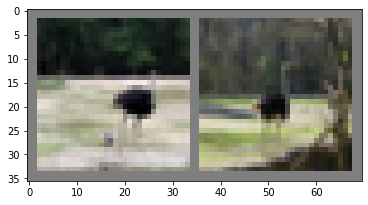
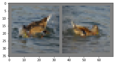
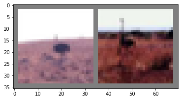
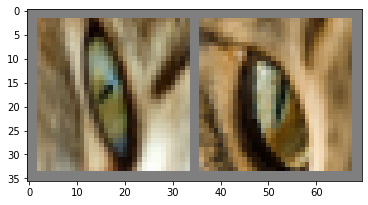
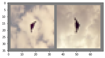
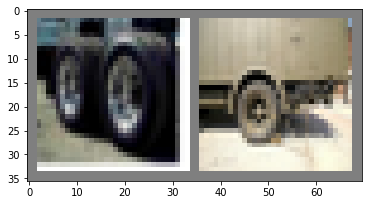
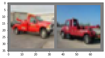
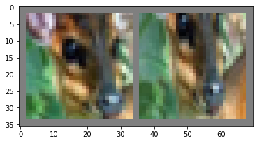
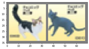
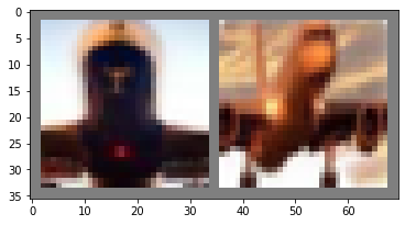
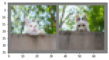
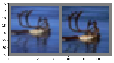
We demonstrate this effect in Figure 7 with examples from CIFAR10 and MNIST. Each pair of images contains a mis-classified (by robustly trained models) test image and the mis-classified training image “responsible” for it (We describe below how they were identified.). Importantly both of these images were correctly classified by a naturally trained model. Visually, it is evident that the training images are extremely similar to the corresponding test image. Inspecting the rest of the training set, they are also very different from other images in the training set. We can thus refer to these as rare sub-populations.
The notion that certain test examples were not classified correctly due to a particular training examples not being classified correctly is measured by the influence a training image has on the test image (c.f. defn 3 in Zhang and Feldman [61]). Intuitively, it measures the probability that a certain test example would be classified correctly if the model were learned using a training set that did not contain the training point compared to if the training set did contain that particular training point. We obtained the influence of each training image on each test image for that class from Zhang and Feldman [61]. We found the images in Figure 7 by manually searching for each test image, the training image that is misclassified and is visually close to it. Our search space was shortened with the help of the influence scores each training image has on the classification of a test image. We searched in the set of top- most influential mis-classified train images for each mis-classified test image. The model used for Figure 7 is a AT model for CIFAR10 with -adversary with an and a model trained with TRADES for MNIST with and .
A precise notion of measuring if a sample is rare is through the concept of self-influence. Self influence of an example with respect to an algorithm (model, optimizer etc) can be defined as how unlikely it is for the model learnt by that algorithm to be correct on an example if it had not seen that example during training compared to if it had seen the example during training. For a precise mathematical definition please refer to Eq (1) in Zhang and Feldman [61]. Self-influence for a rare example, that is unlike other examples of that class, will be high as the rest of the dataset will not provide relevant information that will help the model in correctly predicting on that particular example. In Figure 9, we show that the self-influence of training samples that were mis-classified by adversarially trained models but correctly classified by a naturally trained model is higher compared to the distribution of self-influence on the entire train dataset. In other words, it means that the self-influence of the training examples mis-classified by the robustly trained models is larger than the average self-influence of (all) examples belonging to that class. This supports our hypothesis that adversarial training excludes fitting these rare (or ones that need to be memorized) samples.
Experiments on a synthetic setting
This phenomenon is demonstrated more clearly in a simpler distribution for different NN configurations in Figure 11. We create a binary classification problem on . The data is uniformly supported on non-overlapping circles of varying radiuses. All points in one circle have the same label i.e. it is either blue or red depending on the color of the circle. We train a shallow network with 2 layers and 1000 neurons in each layer (Shallow-Wide NN) and a deep network with 4 layers and 100 neurons in each layer using cross entropy loss and SGD. The background color shows the decision region of the learnt neural network. Figure 11 shows that the adversarially trained (AT) models ignore the smaller circles (i.e. rare sub-populations) and tries to get a larger margin around the circles it does classify correctly whereas the naturally trained (NAT) models correctly predicts every circle but ends up with very small margin around a lot of circles.
3.3 Complexity of decision boundaries
When neural networks are trained they create classifiers whose decisions boundaries are much simpler than they need to be for being adversarially robust. A few recent papers [40, 48] have discussed that robustness might require more complex classifiers. In Theorem 2 and 3 we discussed this theoretically and also why this might not violate the traditional wisdom of Occam’s Razor. In particular, complex decision boundaries does not necessarily mean more complex classifiers in statistical notions of complexity like VC dimension. In this section, we show through a simple experiment how the decision boundaries of neural networks are not “complex” enough to provide large enough margins and are thus adversarially much more vulnerable than is possible.
We train three different neural networks with ReLU activations, a shallow network (Shallow NN) with 2 layers and 100 neurons in each layer, a shallow network with 2 layers and 1000 neurons in each layer (Shallow-Wide NN), and a deep network with 4 layers and 100 neurons in each layer. We train them for 200 epochs on a binary classification problem as constructed in Figure 12. The distribution is supported on blobs and the color of each blob represent its label. On the right side, we have the decision boundary of a large margin classifier, which is simulated using a 1-nearest neighbour.
From Figure 12, it is evident that the decision boundaries of neural networks trained with standard optimizers have far simpler decision boundaries than is needed to be robust (eg. the 1- nearest neighbour is much more robust than the neural networks.)
3.3.1 Accounting for fine grained sub-populations leads to better robustness
We hypothesize that learning more meaningful representations by accounting for fine-grained sub-populations within each class may lead to better robustness. We use the theoretical setup presented in Section 2.2 and 2(b). However, if each of the circles belonged to a separate class then the decision boundary would have to be necessarily more complex as it needs to, now, separate the balls that were previously within the same class. We test this hypothesis with two experiments. First, we test it on the the distribution defined in Theorem 2 where for each ball with label , we assign it a different label (say ) and similarly for balls with label , we assign it a different label (). Now, we solve a multi-class classification problem for classes with a deep neural network and then later aggregate the results by reporting all s as and all s as .The resulting decision boundary is drawn in Figure 14(a) along with the decision boundary for natural training and AT. Clearly, the decision boundary for AT is the most complex and has the highest margin (and robustness) followed by the multi-class model and then the naturally trained model.
Second, we also repeat the experiment with CIFAR-100. We train a ResNet50 [21] on the fine labels of CIFAR100 and then aggregate the fine labels corresponding to a coarse label by summing up the logits. We call this model the Fine2Coarse model and compare the adversarial risk of this network to a ResNet-50 trained directly on the coarse labels. Note that the model is end-to-end differentiable as the only addition is a layer to aggregate the logits corresponding to the fine classes pertaining to each coarse class. Thus PGD adversarial attacks can be applied out of the box. Figure 14(b) shows that for all perturbation budgets, Fine2Coarse has smaller adversarial risk than the naturally trained model.
4 Related Work
[37] established that there are concept classes with finite VC dimensions i.e. are properly PAC-learnable but are only improperly robustly PAC learnable. This implies that to learn the problem with small adversarial error, a different class of models (or representations) needs to be used whereas for small natural test risk, the original model class (or representation) can be used. Recent empirical works have also shown evidence towards this (eg. [46]).
Hanin and Rolnick [18] have shown that though the number of possible linear regions that can be created by a deep ReLU network is exponential in depth, in practice for networks trained with SGD this tends to grow only linearly thus creating much simpler decision boundaries than is possible due to sheer expresssivity of deep networks. Experiments on the data models from our theoretical settings indeed show that adversarial training indeed produces more “complex” decision boundaries
Jacobsen et al. [25] have discussed that excesssive invariance in neural networks might increase adversarial error. However, their argument is that excessive invariance can allow sufficient changes in the semantically important features without changing the network’s prediction. They describe this as Invariance-based adversarial examples as opposed to perturbation based adversarial examples. We show that excessive (incorrect) invariance might also result in perturbation based adversarial examples.
Another contemporary work [15] discusses a phenomenon they refer to as Shortcut Learning where deep learning models perform very well on standard tasks like reducing classification error but fail to perform in more difficult real world situations. We discuss this in the context of models that have small test error but large adversarial error and provide and theoretical and empirical to discuss why one of the reasons for this is sub-optimal representation learning.
5 Conclusion
Recent research has largely shone a positive light on interpolation (zero training error) by highly over-parameterized models even in the presence of label noise. While overfitting noisy data may not harm generalisation, we have shown that this can be severely detrimental to robustness. This raises a new security threat where label noise can be inserted into datasets to make the models learnt from them vulnerable to adversarial attacks without hurting their test accuracy. As a result, further research into learning without memorization is ever more important [47, 50]. Further, we underscore the importance of proper representation learning in regards to adversarial robustness. Representations learnt by deep networks often encode a lot of different invariances, e.g., location, permutation, rotation, etc. While some of them are useful for the particular task at hand, we highlight that certain invariances can increase adversarial vulnerability. Thus we believe that making significant progress towards training robust models with good test error requires us to rethink representation learning and closely examine the data on which we are training these models.
6 Acknowledgement
We thank Vitaly Feldman and Chiyuan Zhang for providing us with data that helped to significantly speed up some parts of this work. We also thank Nicholas Lord for feedback on the draft. AS acknowledges support from The Alan Turing Institute under the Turing Doctoral Studentship grant TU/C/000023. VK is supported in part by the Alan Turing Institute under the EPSRC grant EP/N510129/1. PHS and PD are supported by the ERC grant ERC-2012-AdG 321162-HELIOS, EPSRC grant Seebibyte EP/M013774/1 and EPSRC/MURI grant EP/N019474/1. PHS and PD also acknowledges the Royal Academy of Engineering and FiveAI.
Appendix A Proofs for Section 2
In this section, we present the formal proofs to the theorems stated in Section 2.
A.1 Proof of Theorem 1
See 1
Proof of Theorem 1.
From eq. 3, for any and ,
As the sampling of the point and the injection of label noise are independent events,
Thus,
Substituting and applying the union bound over all , we get
| (4) |
As for all and , we have that
where is the true concept for the distribution . The second equality follows from the assumptions that each of the balls around are pure in their labels. The second last equality follows from eq. 4 by using the that is guaranteed to exist in the ball around and be mis-labelled with probability atleast . The last equality from Assumption eq. 4. ∎
A.2 Proofs of Section 2.2
See 2
Proof of Theorem 2.
We define a family of distribution , such that each distribution in is supported on balls of radius around and for positive integers . Either all the balls around have the labels and the balls around have the label or vice versa. Figure 2(b) shows an example where the colors indicate the label.
Formally, for , , the -1 bit parity class conditional model is defined over as follows. First, a label is sampled uniformly from , then and integer is sampled uniformly from the set and finally is generated by sampling uniformly from the ball of radius around .
In Lemma 1 we first show that a set of points sampled iid from any distribution as defined above for is with probability linear separable for any . In addition, standard VC bounds show that any linear classifier that separates for large enough will have small test error. Lemma 1 also proves that there exists a range of such that for any distribution defined with in that range, though it is possible to obtain a linear classifier with training and test error, the minimum adversarial risk will be bounded from .
However while it is possible to obtain a linear classifier with test error, all such linear classifiers has a large adversarial vulnerability. In Lemma 2, we show that there exists a different representation for this problem, which also achieves zero training and test error and in addition has zero adversarial risk for a range of where the linear classifier’s adversarial error was atleast a constant.
∎
Lemma 1 (Linear Classifier).
There exists universal constants , such that for any perturbation , radius , and , the following holds. Let be the family of - 1-bit parity class conditional model, and be a set of points sampled i.i.d. from .
-
1)
For any , is linearly separable with probability i.e. there exists a , such that the linear hyperplane separates with probability :
-
2)
Further there exists an universal constant such that for any with probability for any with , any linear classifier that separates has .
-
3)
Let be any linear classifier that has . Then, .
We will prove the first part for any by constructing a such that it satisfies the constraints of linear separability. Let . Consider any point and . Converting to the polar coordinate system there exists a such that
Part 2 follows with simple VC bounds of linear classifiers.
Let the universal constants be and respectively. Note that there is nothing special about this constants except that some constant is required to bound the adversarial risk away from . Now, consider a distribution 1-bit parity model such that the radius of each ball is atleast . This is smaller than and thus satisfies the linear separability criterion.
Consider to be a hyper-plane that has test error. Let the radius of adversarial perturbation be . The region of each circle that will be vulnerable to the attack will be a circular segment with the chord of the segment parallel to the hyper-plane. Let the minimum height of all such circular segments be . Thus, is greater than the mass of the circular segment of radius . Let the radius of each ball in the support of be .
Using the fact that has zero test error; and thus classifies the balls in the support of correctly and simple geometry
| (5) |
To compute we need to compute the ratio of the area of a circular segment of height of a circle of radius to the area of the circle. The ratio can be written
| (6) |
As Equation 6 is increasing with , we can evaluate
| UsingEquation 5 | ||||
Substituting into Eq. Equation 6, we get that . Thus, for all , we have .
Lemma 2 (Robustness of parity classifier).
There exists a concept class such that for any , , being the corresponding 1-bit parity class distribution where are the same as in Lemma 1 there exists such that
Proof of Lemma 2.
We will again provide a proof by construction. Consider the following class of concepts such that is defined as
| (7) |
where rounds to the nearest integer and . In Figure 2(b), the green staircase-like classifier belongs to this class. Consider the classifier . Note that by construction . The decision boundary of that are closest to a ball in the support of centered at are the lines and .
As , the adversarial perturbation is upper bounded by . The radius of the ball is upper bounded by , and as we noted the center of the ball is at a distance of from the decision boundary. If the sum of the maximum adversarial perturbation and the maximum radius of the ball is less than the minimum distance of the center of the ball from the decision boundary, then the adversarial error is . Substituting the values,
This completes the proof. ∎
Appendix B Proof of Section 2.3
See 3
Proof of Theorem 3.
We will provide a constructive proof to this theorem by constructing a distribution , two concept classes and and provide the ERM algorithms to learn the concepts and then use Lemma 3 and 4 to complete the proof.
Distribution: Consider the family of distribution such that is defined on for such that the support of is a union of intervals.
| (8) |
We consider distributions with a relatively small support i.e. where . Each sample is created by sampling uniformly from and assigning where is defined below eq. 9. We define the family of distributions . Finally, we create -a noisy version of , by flipping in each sample with probability . Samples from can be obtained using the example oracle and samples from the noisy distribution can be obtained through the noisy oracle
Concept Class : We define the concept class of concepts such that
| (9) |
where rounds a decimal to its nearest integer, returns the binary encoding of the integer, and . is the least significant bit in the binary encoding of the nearest integer to . It is essentially the class of parity functions defined on the bits corresponding to the indices in for the binary encoding of the nearest integer to . For example, as in Figure 2(a) if , then only the least significant and the third least significant bit of are examined and the class label is if an odd number of them are and otherwise.
Concept Class : Finally, we define the concept class where is the class of union of intervals on the real line . Each concept can be written as a set of disjoint intervals on the real line i.e. for , where and
| (10) |
Now, we look at the algorithms to learn the concepts from and that minimize the train error. Both of the algorithms will use a majority vote to determine the correct (de-noised) label for each interval, which will be necessary to minimize the test error. The intuition is that if we draw a sufficiently large number of samples, then the majority of samples on each interval will have the correct label with a high probability.
Lemma 3 proves that there exists an algorithm such that draws samples from the noisy oracle and with probability where the probability is over the randomization in the oracle, returns such that and for all . As Lemma 3 states, the algorithm involves gaussian elimination over variables and majority votes (one in each interval) involving a total of samples. Thus the algorithm runs in time. Replacing the complexity of and the fact that , the complexity of the algorithm is .
Lemma 4 proves that there exists an algorithm such that draws
samples and returns such that has training error, test error and an adversarial test error of atleast . We can replace to get the required bound on in the theorem. The algorithm to construct visits every point atmost twice - once during the construction of the intervals using majority voting, and once while accommodating for the mislabelled points. Replacing the complexity of , the complexity of the algorithm is . This completes the proof. ∎
Lemma 3 (Parity Concept Class).
There exists a learning algorithm such that given access to the noisy example oracle , makes calls to the oracle and returns a hypothesis such that with probability , we have that and for all .
Proof.
The algorithm works as follows. It makes calls to the oracle to obtain a set of points where . Then, it replaces each with ( rounds a decimal to the nearest integer) and then removes duplicate s by preserving the most frequent label associated with each . For example, if then after this operation, we will have .
As , using and in Lemma 5 guarantees that with probability , each interval will have atleast samples.
Then for any specific interval, using in Lemma 6 guarantees that with probability atleast , the majority vote for the label in that interval will succeed in returning the de-noised label. Applying a union bound over all intervals, will guarantee that with probability atleast , the majority label of every interval will be the denoised label.
Now, the problem reduces to solving a parity problem on this reduced dataset of points (after denoising, all points in that interval can be reduced to the integer in the interval and the denoised label). We know that there exists a polynomial algorithm using Gaussian Elimination that finds a consistent hypothesis for this problem. We have already guaranteed that there is a point in from every interval in the support of . Further, is consistent on and is constant in each of these intervals by design. Thus, with probability atleast we have that .
By construction, makes a constant prediction on each interval for all . Thus, for any perturbation radius the adversarial risk . Combining everything, we have shown that there is an algorithm that makes calls to the oracle, runs in time polynomial in to return such that and for . ∎
Lemma 4 (Union of Interval Concept Class).
There exists a learning algorithm such that given access to a noisy example oracle makes calls to the oracle and returns a hypothesis such that training error is and with probability , .
Further for any that has zero training error on samples drawn from for and then for all .
Proof of Lemma 4.
The first part of the algorithm works similarly to Lemma 3. The algorithm makes calls to the oracle to obtain a set of points where . computes as follows. To begin, let the list of intervals in be and Then do the following for every .
-
1.
let ,
-
2.
Let be the set of all such that .
-
3.
Compute the majority label of .
-
4.
Add all such that to
-
5.
If , then add the interval to .
-
6.
Remove all elements of from i.e. .
For reasons similar to Lemma 3, as , Lemma 5 guarantees that with probability , each interval will have atleast samples. Then for any specific interval, Lemma 6 guarantees that with probability atleast , the majority vote for the label in that interval will succeed in returning the de-noised label. Applying a union bound over all intervals, will guarantee that with probability atleast , the majority label of every interval will be the denoised label. As each interval in has atleast one point, all the intervals in with label will be included in with probability . Thus, .
Now, for all , add the interval to if . If then must lie a interval . Replace that interval as follows . As only a finite number of sets with lebesgue measure of were added or deleted from , the net test error of doesn’t change and is still i.e.
For the second part, we will invoke Theorem 1. To avoid confusion in notation, we will use instead of to refer to the sets in Theorem 1 and reserve for the support of interval of . Let be any set of disjoint intervals of width such that . This is always possible as the total width of all intervals in is which is less than the total width of the support . from Eq. Equation 3 is
Thus, if has an error of zero on a set of examples drawn from where , then by Theorem 1, .
Combining the two parts for
it is possible to obtain such that has zero training error, and for any .
∎
Lemma 5.
Given and a distribution , for any if samples are drawn from then with probability atleast there are atleast samples in each interval for all .
Proof of Lemma 5.
We will repeat the following procedure times once for each interval in and show that with probability the run will result in atleast samples in the interval.
Corresponding to each interval in , we will sample atleast samples where . If is the random variable that is when the sample belongs to the interval, then interval has atleast points out of the points sampled for that interval with probability less than .
| By Chernoff’s inequality | ||||
where the last step follows from . With probability atleast , every interval will have atleast samples. Finally, an union bound over each interval gives the desired result. As we repeat the process for all intervals, the total number of samples drawn will be atleast . ∎
Lemma 6 (Majority Vote).
For a given , let be a set of size where each element is with probability and otherwise. If then with probability atleast the majority of is .
Proof of Lemma 6.
Without loss of generality let . For the majority to be we need to show that there are more than “”s in i.e. we need to show that the following probability is less than .
| By Chernoff’s Inequality | ||||
∎
References
- Athalye et al. [2018] A. Athalye, N. Carlini, and D. Wagner. Obfuscated gradients give a false sense of security: Circumventing defenses to adversarial examples. In Proceedings of the 35th International Conference on Machine Learning, ICML 2018, July 2018. URL https://arxiv.org/abs/1802.00420.
- Bartlett et al. [2020] P. L. Bartlett, P. M. Long, G. Lugosi, and A. Tsigler. Benign overfitting in linear regression. Proceedings of the National Academy of Sciences, page 201907378, apr 2020. doi: 10.1073/pnas.1907378117.
- Belkin et al. [2018a] M. Belkin, D. J. Hsu, and P. Mitra. Overfitting or perfect fitting? risk bounds for classification and regression rules that interpolate. In S. Bengio, H. Wallach, H. Larochelle, K. Grauman, N. Cesa-Bianchi, and R. Garnett, editors, Advances in Neural Information Processing Systems 31, pages 2300–2311. Curran Associates, Inc., 2018a. URL http://papers.nips.cc/paper/7498-overfitting-or-perfect-fitting-risk-bounds-for-classification-and-regression-rules-that-interpolate.pdf.
- Belkin et al. [2018b] M. Belkin, S. Ma, and S. Mandal. To understand deep learning we need to understand kernel learning. In J. Dy and A. Krause, editors, Proceedings of the 35th International Conference on Machine Learning, volume 80 of Proceedings of Machine Learning Research, pages 541–549, Stockholmsmässan, Stockholm Sweden, 10–15 Jul 2018b. PMLR. URL http://proceedings.mlr.press/v80/belkin18a.html.
- Belkin et al. [2019a] M. Belkin, D. Hsu, and J. Xu. Two models of double descent for weak features. arXiv:1903.07571, 2019a.
- Belkin et al. [2019b] M. Belkin, A. Rakhlin, and A. B. Tsybakov. Does data interpolation contradict statistical optimality? In K. Chaudhuri and M. Sugiyama, editors, Proceedings of Machine Learning Research, volume 89 of Proceedings of Machine Learning Research, pages 1611–1619. PMLR, 16–18 Apr 2019b. URL http://proceedings.mlr.press/v89/belkin19a.html.
- Biggio and Roli [2018] B. Biggio and F. Roli. Wild patterns. In Proceedings of the 2018 ACM SIGSAC Conference on Computer and Communications Security. ACM, jan 2018. doi: 10.1145/3243734.3264418.
- Carlini and Wagner [2017a] N. Carlini and D. Wagner. Towards evaluating the robustness of neural networks. In 2017 IEEE Symposium on Security and Privacy (SP). IEEE, may 2017a. doi: 10.1109/sp.2017.49.
- Carlini and Wagner [2017b] N. Carlini and D. Wagner. Adversarial examples are not easily detected. In Proceedings of the 10th ACM Workshop on Artificial Intelligence and Security -. ACM Press, 2017b. doi: 10.1145/3128572.3140444.
- Chatterji and Long [2020] N. S. Chatterji and P. M. Long. Finite-sample analysis of interpolating linear classifiers in the overparameterized regime. arXiv:2004.12019, 2020.
- Cisse et al. [2017] M. Cisse, P. Bojanowski, E. Grave, Y. Dauphin, and N. Usunier. Parseval networks: Improving robustness to adversarial examples. In D. Precup and Y. W. Teh, editors, Proceedings of the 34th International Conference on Machine Learning, volume 70 of Proceedings of Machine Learning Research, pages 854–863, International Convention Centre, Sydney, Australia, 06–11 Aug 2017. PMLR. URL http://proceedings.mlr.press/v70/cisse17a.html.
- Dalvi et al. [2004] N. Dalvi, P. Domingos, Mausam, S. Sanghai, and D. Verma. Adversarial classification. In Proceedings of the 2004 ACM SIGKDD international conference on Knowledge discovery and data mining - KDD2004. ACM Press, 2004. doi: 10.1145/1014052.1014066.
- Degwekar et al. [2019] A. Degwekar, P. Nakkiran, and V. Vaikuntanathan. Computational limitations in robust classification and win-win results. In A. Beygelzimer and D. Hsu, editors, Proceedings of the Thirty-Second Conference on Learning Theory, volume 99 of Proceedings of Machine Learning Research, pages 994–1028, Phoenix, USA, 25–28 Jun 2019. PMLR. URL http://proceedings.mlr.press/v99/degwekar19a.html.
- Feldman [2019] V. Feldman. Does learning require memorization? a short tale about a long tail. arXiv:1906.05271, 2019.
- [15] R. Geirhos, J.-H. Jacobsen, C. Michaelis, R. Zemel, W. Brendel, M. Bethge, and F. A. Wichmann. Shortcut learning in deep neural networks.
- Goodfellow et al. [2014] I. J. Goodfellow, J. Shlens, and C. Szegedy. Explaining and Harnessing Adversarial Examples. arXiv preprint arXiv:1412.6572, dec 2014. URL http://arxiv.org/abs/1412.6572.
- Graves et al. [2013] A. Graves, A.-r. Mohamed, and G. Hinton. Speech recognition with deep recurrent neural networks. In 2013 IEEE international conference on acoustics, speech and signal processing, pages 6645–6649. IEEE, 2013.
- Hanin and Rolnick [2019] B. Hanin and D. Rolnick. Complexity of linear regions in deep networks. In K. Chaudhuri and R. Salakhutdinov, editors, Proceedings of the 36th International Conference on Machine Learning, volume 97 of Proceedings of Machine Learning Research, pages 2596–2604, Long Beach, California, USA, 09–15 Jun 2019. PMLR. URL http://proceedings.mlr.press/v97/hanin19a.html.
- Hastie et al. [2019] T. Hastie, A. Montanari, S. Rosset, and R. J. Tibshirani. Surprises in high-dimensional ridgeless least squares interpolation. arXiv:1903.08560, 2019.
- He et al. [2015] K. He, X. Zhang, S. Ren, and J. Sun. Delving deep into rectifiers: Surpassing human-level performance on imagenet classification. In Proceedings of the IEEE international conference on computer vision, pages 1026–1034, 2015.
- He et al. [2016] K. He, X. Zhang, S. Ren, and J. Sun. Deep Residual Learning for Image Recognition. In 2016 IEEE Conference on Computer Vision and Pattern Recognition (CVPR), pages 770–778. IEEE, jun 2016. ISBN 978-1-4673-8851-1. doi: 10.1109/CVPR.2016.90. URL http://ieeexplore.ieee.org/document/7780459/.
- He et al. [2017] W. He, J. Wei, X. Chen, N. Carlini, and D. Song. Adversarial example defenses: Ensembles of weak defenses are not strong. In Proceedings of the 11th USENIX Conference on Offensive Technologies, WOOT’17, page 15, USA, 2017. USENIX Association.
- Hendrycks et al. [2019a] D. Hendrycks, K. Lee, and M. Mazeika. Using pre-training can improve model robustness and uncertainty. Proceedings of the International Conference on Machine Learning, 2019a.
- Hendrycks et al. [2019b] D. Hendrycks, K. Zhao, S. Basart, J. Steinhardt, and D. Song. Natural adversarial examples. arXiv:1907.07174, 2019b.
- Jacobsen et al. [2019] J.-H. Jacobsen, J. Behrmann, R. Zemel, and M. Bethge. Excessive invariance causes adversarial vulnerability. In International Conference on Learning Representations, 2019. URL https://openreview.net/forum?id=BkfbpsAcF7.
- Kamath et al. [2020] S. Kamath, A. Deshpande, and K. V. Subrahmanyam. Invariance vs robustness of neural networks. 2020. URL https://openreview.net/forum?id=HJxp9kBFDS.
- Krizhevsky and Hinton [2009] A. Krizhevsky and G. Hinton. Learning multiple layers of features from tiny images. Technical report, Citeseer, 2009.
- Krizhevsky et al. [2012] A. Krizhevsky, I. Sutskever, and G. E. Hinton. Imagenet classification with deep convolutional neural networks. In Advances in neural information processing systems, pages 1097–1105, 2012.
- Kurakin et al. [2016] A. Kurakin, I. Goodfellow, and S. Bengio. Adversarial examples in the physical world. arXiv preprint arXiv:1607.02533, 2016.
- Kurakin et al. [2017] A. Kurakin, I. Goodfellow, and S. Bengio. Adversarial machine learning at scale. International Conference on Learning Representations (ICLR), 2017.
- LeCun et al. [1998] Y. LeCun, L. Bottou, Y. Bengio, and P. Haffner. Gradient-based learning applied to document recognition. Proceedings of the IEEE, 86(11):2278–2324, 1998.
- Li et al. [2019a] J. Li, F. Schmidt, and Z. Kolter. Adversarial camera stickers: A physical camera-based attack on deep learning systems. In K. Chaudhuri and R. Salakhutdinov, editors, Proceedings of the 36th International Conference on Machine Learning, volume 97 of Proceedings of Machine Learning Research, pages 3896–3904, Long Beach, California, USA, 09–15 Jun 2019a. PMLR. URL http://proceedings.mlr.press/v97/li19j.html.
- Li et al. [2019b] M. Li, M. Soltanolkotabi, and S. Oymak. Gradient descent with early stopping is provably robust to label noise for overparameterized neural networks. arXiv:1903.11680, 2019b.
- Liang and Rakhlin [2018] T. Liang and A. Rakhlin. Just interpolate: Kernel ”ridgeless” regression can generalize. arXiv:1808.00387, 2018.
- Liu et al. [2018] R. Liu, J. Lehman, P. Molino, F. P. Such, E. Frank, A. Sergeev, and J. Yosinski. An intriguing failing of convolutional neural networks and the coordconv solution. In S. Bengio, H. M. Wallach, H. Larochelle, K. Grauman, N. Cesa-Bianchi, and R. Garnett, editors, Advances in Neural Information Processing Systems 31: Annual Conference on Neural Information Processing Systems 2018, NeurIPS 2018, 3-8 December 2018, Montréal, Canada, pages 9628–9639, 2018. URL http://papers.nips.cc/paper/8169-an-intriguing-failing-of-convolutional-neural-networks-and-the-coordconv-solution.
- Madry et al. [2018] A. Madry, A. Makelov, L. Schmidt, D. Tsipras, and A. Vladu. Towards deep learning models resistant to adversarial attacks. In International Conference on Learning Representations, 2018. URL https://openreview.net/forum?id=rJzIBfZAb.
- Montasser et al. [2019] O. Montasser, S. Hanneke, and N. Srebro. Vc classes are adversarially robustly learnable, but only improperly. In A. Beygelzimer and D. Hsu, editors, Proceedings of the Thirty-Second Conference on Learning Theory, volume 99 of Proceedings of Machine Learning Research, pages 2512–2530, Phoenix, USA, 25–28 Jun 2019. PMLR. URL http://proceedings.mlr.press/v99/montasser19a.html.
- Moosavi-Dezfooli et al. [2016] S.-M. Moosavi-Dezfooli, A. Fawzi, and P. Frossard. DeepFool: {A} Simple and Accurate Method to Fool Deep Neural Networks. In CVPR, pages 2574–2582. {IEEE} Computer Society, 2016.
- Muthukumar et al. [2020] V. Muthukumar, K. Vodrahalli, V. Subramanian, and A. Sahai. Harmless interpolation of noisy data in regression. IEEE Journal on Selected Areas in Information Theory, pages 1–1, 2020. doi: 10.1109/jsait.2020.2984716.
- Nakkiran [2019] P. Nakkiran. Adversarial robustness may be at odds with simplicity. arXiv preprintarXiv:1901.00532, 2019.
- Papernot et al. [2015] N. Papernot, P. McDaniel, X. Wu, S. Jha, and A. Swami. Distillation as a defense to adversarial perturbations against deep neural networks. arXiv:1511.04508, 2015.
- Papernot et al. [2016] N. Papernot, P. McDaniel, and I. Goodfellow. Transferability in machine learning: from phenomena to black-box attacks using adversarial samples. arXiv:1605.07277, 2016.
- Papernot et al. [2017] N. Papernot, P. McDaniel, I. Goodfellow, S. Jha, Z. B. Celik, and A. Swami. Practical black-box attacks against machine learning. In Proceedings of the 2017 ACM on Asia Conference on Computer and Communications Security. ACM, apr 2017. doi: 10.1145/3052973.3053009.
- Raghunathan et al. [2019] A. Raghunathan, S. M. Xie, F. Yang, J. C. Duchi, and P. Liang. Adversarial training can hurt generalization. arXiv:1906.06032, 2019.
- Ren et al. [2015] S. Ren, K. He, R. Girshick, and J. Sun. Faster r-cnn: Towards real-time object detection with region proposal networks. In Advances in neural information processing systems, pages 91–99, 2015.
- Sanyal et al. [2020a] A. Sanyal, P. K. Dokania, V. Kanade, and P. Torr. Robustness via deep low-rank representations. https://arxiv.org/abs/1804.07090, 2020a.
- Sanyal et al. [2020b] A. Sanyal, P. H. Torr, and P. K. Dokania. Stable rank normalization for improved generalization in neural networks and {gan}s. In International Conference on Learning Representations, 2020b. URL https://openreview.net/forum?id=H1enKkrFDB.
- Schmidt et al. [2018] L. Schmidt, S. Santurkar, D. Tsipras, K. Talwar, and A. Madry. Adversarially robust generalization requires more data. In Advances in Neural Information Processing Systems, pages 5014–5026, 2018.
- Schönherr et al. [2018] L. Schönherr, K. Kohls, S. Zeiler, T. Holz, and D. Kolossa. Adversarial attacks against automatic speech recognition systems via psychoacoustic hiding. arXiv:1808.05665, 2018.
- Shen and Sanghavi [2019] Y. Shen and S. Sanghavi. Learning with bad training data via iterative trimmed loss minimization. In K. Chaudhuri and R. Salakhutdinov, editors, Proceedings of the 36th International Conference on Machine Learning, volume 97 of Proceedings of Machine Learning Research, pages 5739–5748, Long Beach, California, USA, 09–15 Jun 2019. PMLR. URL http://proceedings.mlr.press/v97/shen19e.html.
- Szegedy et al. [2013] C. Szegedy, W. Zaremba, I. Sutskever, J. Bruna, D. Erhan, I. Goodfellow, and R. Fergus. Intriguing properties of neural networks. arXiv preprint arXiv:1312.6199, 2013.
- Tramer et al. [2020] F. Tramer, N. Carlini, W. Brendel, and A. Madry. On adaptive attacks to adversarial example defenses. arXiv:2002.08347, 2020.
- Tramèr et al. [2018] F. Tramèr, A. Kurakin, N. Papernot, I. Goodfellow, D. Boneh, and P. McDaniel. Ensemble adversarial training: Attacks and defenses. In International Conference on Learning Representations, 2018. URL https://openreview.net/forum?id=rkZvSe-RZ.
- Tsipras et al. [2019] D. Tsipras, S. Santurkar, L. Engstrom, A. Turner, and A. Madry. Robustness may be at odds with accuracy. In International Conference on Learning Representations, 2019. URL https://openreview.net/forum?id=SyxAb30cY7.
- Vaswani et al. [2017] A. Vaswani, N. Shazeer, N. Parmar, J. Uszkoreit, L. Jones, A. N. Gomez, Ł. Kaiser, and I. Polosukhin. Attention is all you need. In Advances in neural information processing systems, pages 5998–6008, 2017.
- Wong et al. [2020] E. Wong, L. Rice, and J. Z. Kolter. Fast is better than free: Revisiting adversarial training. In International Conference on Learning Representations, 2020. URL https://openreview.net/forum?id=BJx040EFvH.
- Xu et al. [2017] W. Xu, D. Evans, and Y. Qi. Feature squeezing: Detecting adversarial examples in deep neural networks. arXiv:1704.01155, 2017. doi: 10.14722/ndss.2018.23198.
- Yang et al. [2020] Y.-Y. Yang, C. Rashtchian, H. Zhang, R. Salakhutdinov, and K. Chaudhuri. Adversarial robustness through local lipschitzness. arXiv:2003.02460, 2020.
- Yin et al. [2019] D. Yin, R. Kannan, and P. Bartlett. Rademacher complexity for adversarially robust generalization. In K. Chaudhuri and R. Salakhutdinov, editors, Proceedings of the 36th International Conference on Machine Learning, volume 97 of Proceedings of Machine Learning Research, pages 7085–7094, Long Beach, California, USA, 09–15 Jun 2019. PMLR. URL http://proceedings.mlr.press/v97/yin19b.html.
- Zagoruyko and Komodakis [2016] S. Zagoruyko and N. Komodakis. Wide residual networks. In Procedings of the British Machine Vision Conference 2016. British Machine Vision Association, 2016. doi: 10.5244/c.30.87.
- Zhang and Feldman [2020] C. Zhang and V. Feldman. What neural networks memorize and why: Discovering the long tail via influence estimation. 2020. URL http://vtaly.net/papers/FZ_Infl_mem.pdf. Unpublished manuscript.
- Zhang et al. [2016] C. Zhang, S. Bengio, M. Hardt, B. Recht, and O. Vinyals. Understanding deep learning requires rethinking generalization. International Conference on Learning Representations (ICLR), nov 2016. URL http://arxiv.org/abs/1611.03530.
- Zhang et al. [2019] H. Zhang, Y. Yu, J. Jiao, E. P. Xing, L. E. Ghaoui, and M. I. Jordan. Theoretically principled trade-off between robustness and accuracy. In K. Chaudhuri and R. Salakhutdinov, editors, Proceedings of the 36th International Conference on Machine Learning, ICML 2019, 9-15 June 2019, Long Beach, California, USA, volume 97 of Proceedings of Machine Learning Research, pages 7472–7482. PMLR, 2019. URL http://proceedings.mlr.press/v97/zhang19p.html.