The ALMA-PILS survey: First detection of the unsaturated 3-carbon molecules Propenal (C₂H₃CHO) and Propylene (C₃H₆) towards IRAS 16293–2422 B

Abstract

Context. Complex organic molecules with three carbon atoms are found in the earliest stages of star formation. In particular, propenal (C₂H₃CHO) is a species of interest due to its implication in the formation of more complex species and even biotic molecules.

Aims. This study aims to search for the presence of C₂H₃CHO and other three-carbon species such as propylene (C₃H₆) in the hot corino region of the low-mass protostellar binary IRAS 16293–2422 to understand their formation pathways.

Methods. We use ALMA observations in Band 6 and 7 from various surveys to search for the presence of C₃H₆ and C₂H₃CHO towards the protostar IRAS 16293–2422 B (IRAS 16293B). The identification of the species and the estimates of the column densities and excitation temperatures are carried out by modeling the observed spectrum under the assumption of local thermodynamical equilibrium.

Results. We report the detection of both C₃H₆ and C₂H₃CHO towards IRAS 16293B, however, no unblended lines were found towards the other component of the binary system, IRAS 16293A. We derive column density upper limits for C₃H₈, HCCCHO, n-C₃H₇OH, i-C₃H₇OH, C₃O, and cis-HC(O)CHO towards IRAS 16293B. We then use a three-phase chemical model to simulate the formation of these species in a typical prestellar environment followed by its hydrodynamical collapse until the birth of the central protostar. Different formation paths, such as successive hydrogenation and radical-radical additions on grain surfaces, are tested and compared to the observational results in a number of different simulations, to assess which are the dominant formation mechanisms in the most embedded region of the protostar.

Conclusions. The simulations reproduce the abundances within one order of magnitude from those observed towards IRAS 16293B, with the best agreement found for a rate of $10^{-12}$ cm³ s^-1 for the gas-phase reaction C₃ + O $\rightarrow$ C₂ + CO. Successive hydrogenations of C₃, HC(O)CHO, and CH₃OCHO on grain surfaces are a major and crucial formation route of complex organics molecules, whereas both successive hydrogenation pathways and radical-radical addition reactions contribute to the formation of C₂H₅CHO.

1 Introduction

Aldehyde molecules, which contain a functional group CHO, play an important role in the formation of complex organic molecules (COMs, molecules containing six or more atoms with at least one carbon, Herbst & van Dishoeck 2009). The two-carbon to three-carbon chain aldehydes are generally found in the cold dense regions of star formation as well as in the innermost warm region of protostellar envelope, the hot core. In particular, propenal (C₂H₃CHO), also called acrolein, is considered as a prebiotic species due to its formation after the decomposition of sugars (Moldoveanu 2010; Bermúdez et al. 2013) and its role in the synthesis of amino acids via Strecker-type reactions (Strecker 1850, 1854) as tested in laboratory studies (e.g. van Trump & Miller 1972; Shibasaki et al. 2008; Grefenstette 2017). On the other hand, on the primordial Earth, C₂H₃CHO is one of a few species that readily reacts with nucleobases of the ribonucleic acid (RNA, Nelsestuen 1980), which makes it a possible sink for the nucleobases and an important hindrance to the start of the RNA world (e.g. Gargaud et al. 2007; Neish et al. 2010). Propynal (HCCCHO), C₂H₃CHO and propanal (C₂H₅CHO) are suspected to be linked through their formation on ice surfaces by successive hydrogenation (e.g. Hudson & Moore 1999). C₂H₃CHO and C₂H₅CHO were first detected in the interstellar medium toward the Galactic Center source Sgr B2(N) (Hollis et al. 2004; Requena-Torres et al. 2008), while HCCCHO was first detected towards the dark cloud TMC–1 (Irvine et al. 1988; Turner 1991).

Three-carbon-chain molecules have also been observed in the ISM and are, in general, more abundant towards protostars characterised by warm carbon-chain chemistry (WCCC), such as L1527 (Sakai et al. 2008), and cold dense clouds. For example, propylene (C₃H₆) was detected for the first time towards TMC-1 (Marcelino et al. 2007). It has so far never been reported in warmer environments, where COMs are found with high abundances, such as hot cores/corinos, contrary to methyl acetylene (CH₃CCH) already found with high abundances in such objects (e.g. van Dishoeck et al. 1995; Cazaux et al. 2003).

In this paper we report detections of C₂H₃CHO and C₃H₆ towards the low-mass Class 0 protostellar binary IRAS 16293–2422 (IRAS 16293 hereafter). This source, located in the $\rho$ Ophiuchus cloud complex at a distance of 144$\pm$7 pc (Zucker et al. 2019), is well-known as a reference in astrochemistry because of its molecule-rich envelope and the presence of numerous bright emission lines at millimetre wavelengths (for example, van Dishoeck et al. 1995; Cazaux et al. 2003; Caux et al. 2011). The high sensitivity and the high angular resolution of the Atacama Large (sub)Millimeter Array (ALMA) allowed many new detections around solar-type protostars and in the interstellar medium. Using ALMA observations of the Protostellar Interferometric Line Survey (PILS, Jørgensen et al. 2016), some of these new detections of COMs, such as deuterated formamide (NHDCHO and NH₂CDO) and isocyanic acid (HNCO) by Coutens et al. (2016), methyl chloride (CH₃Cl, Fayolle et al. 2017), methyl isocyanate (CH₃NCO, Ligterink et al. 2017), cyanamide (NH₂CN, Coutens et al. 2018b), methyl isocyanide (CH₃NC, Calcutt et al. 2018a), and nitrous acid (HONO, Coutens et al. 2019) have been reported towards this protostellar binary. C₂H₅CHO (Lykke et al. 2017) and CH₃CCH (Calcutt et al. 2019) are also detected in the embedded hot corino towards the “B component” (IRAS 16293B) of this source. This demonstrates the possibility of finding the unsaturated precursors of C₂H₅CHO and provide new constraints on the formation of these species in low-mass protostellar environments. It also suggests the need to develop models to describe these three-carbon species (C₃-species hereafter) using laboratory measurements and theoretical calculations both for the gas phase and grain surfaces (Loison et al. 2014, 2017; Hickson et al. 2016b; Qasim et al. 2019).

This paper is organised as follows: Section 2 describes the observations and the spectroscopic data used in this study. The results and the analysis are presented in Sect. 3. These results are then compared to a chemical model which is described in Sect. 4. Finally, the comparison between the results and the model are discussed in Sect. 5 and the conclusions summarised in Sect. 6.

2 Observations

Table 1: List of the observations towards IRAS 16293B used in this study.

Project	Band	Frequency range	Spectral resolution	Beam size	Sensitivity
		(GHz)	(MHz)	(arcsec)	(mJy beam-1 channel-1)
2012.1.00712.S	Band 6	221.77 – 222.23	0.122	0.5	7 – 10
		224.77 – 225.23
		231.02 – 231.48
		232.16 – 232.62
		239.42 – 239.88
		240.17 – 240.63
		247.30 – 247.76
		250.26 – 250.72
2016.1.01150.S	Band 6	233.71 – 234.18	0.122	0.5	1.2 – 1.4
		234.92 – 235.39
		235.91 – 236.84
2013.1.00278.S	Band 7	329.15 – 362.90	0.244	0.5	7 – 10

Observations at 1.3 and 0.8 mm wavelength, carried out with ALMA, corresponding to Band 6 and 7, respectively, towards IRAS 16293 were used in this study. The pointing centre, located between the two protostars of the binary system at $\alpha_{\text{J2000}}=16^{\text{h}}32^{\text{m}}22{\aas@@fstack{s}}72$; $\delta_{\text{J2000}}=-24^{\circ}28^{\prime}34{\aas@@fstack{\prime\prime}}3$, was the same for all the observations. The species that are the main focus of this study are the C₃-species C₂H₃CHO and C₃H₆, as well as the chemically related species HCCCHO, C₂H₅CHO, propanol (n-C₃H₇OH) and its iso conformer (i-C₃H₇OH), tricarbon monoxide (C₃O), C₃H₈, and glyoxal (cis-HC(O)CHO). Note that the most abundant conformer of HC(O)CHO, trans-HC(O)CHO, has no dipole moment and does not display any pure rotational transitions, thus it cannot be detected at millimetre wavelengths.

2.1 Band 6 observations

The ALMA-Band 6 data are a combination of PILS observations in Cycle 1 (project-id: 2012.1.00712.S, PI: Jørgensen, J. K.) and Cycle 4 observations taken from Taquet et al. (2018) (project-id: 2016.1.01150.S, PI: Taquet, V.). The observations cover a total of $\sim$5.5 GHz spread between 221.7 and 250.7 GHz with a frequency resolution of 0.122 MHz, corresponding to a velocity resolution of $\sim$0.16 km s^-1. The two datasets have been treated the same way and were restored with the same 0$\aas@@fstack{\prime\prime}$5 circular beam as in Band 7. The continuum subtraction and the data calibration are detailed in Jørgensen et al. (2016) and Taquet et al. (2018), for Cycle 1 and Cycle 4 observations, respectively. Calibration uncertainties are better than 5% and the sensitivity reached is 1 – 10 mJy beam^-1 per channel, depending on the observations.

2.2 Band 7 observations

The Band 7 data are taken from the PILS observations (project-id: 2013.1.00278.S, PI: Jørgensen, J. K.) and cover the full range of 329 to 363 GHz at a frequency resolution of 0.244 MHz, which corresponds to $\sim$0.2 km s^-1 in this frequency range, and were restored with a circular beam of 0$\aas@@fstack{\prime\prime}$5. The continuum subtraction and the data reduction are described in Jørgensen et al. (2016). The sensitivity reaches down to 7–10 mJy beam^-1 per channel and the relative calibration uncertainty across the band is $\sim$5%. Table 1 summarises the details of the spectral windows used in this study.

2.3 Spectroscopic data

The spectroscopic data used to identify C₂H₃CHO transitions are taken from the Cologne Database for Molecular Spectroscopy (CDMS, Müller et al. 2001, 2005). The CDMS entry is based on Daly et al. (2015) with additional data from Winnewisser et al. (1975); Cherniak & Costain (1966). The dipole moment was determined by Blom et al. (1984).

The C₃H₆ rotational transitions are taken from its CDMS entry, based on Craig et al. (2016) with numerous additional transition frequencies from Hirota (1966), Pearson et al. (1994) and Wlodarczak et al. (1994). The dipole moment was measured by Lide & Mann (1957). The spectroscopic entry includes the transitions of A and E torsional substate conformers, which arise from the methyl internal rotation splitting.

Five spectroscopic conformers of n-C₃H₇OH exist, distinguished by the orientation of their methyl and OH groups. Ga-n-C₃H₇OH is the lowest vibrational ground state conformer. The CDMS entry used in this study is largely based on Kisiel et al. (2010), with interactions with other conformers studied by Kahn & Bruice (2005) and additional data from Maeda et al. (2006a); White (1975). The entry only takes the Ga- conformer into account. The correction factor corresponding to the contribution of the other conformers is 2.75 at $T_{\mathrm{ex}}$ = 100 K.

The CDMS entries for the two conformers gauche, the energetically lowest, and anti of i-C₃H₇OH are based on Maeda et al. (2006b); Ulenikov et al. (1991); Hirota (1979). Rotation-tunneling interactions between the conformers are incorporated in the Hamiltonian using the formulation described in Christen & Müller (2003). Unlike the n-C₃H₇OH entry, the i-C₃H₇OH partition function already includes the contribution of gauche and anti conformers.

Spectroscopic data of HCCCHO were taken from its CDMS entry, which is based on McKellar et al. (2008) with additional data from Costain & Morton (1959) and Winnewisser (1973). The dipole moment was measured by Brown & Godfrey (1984).

C₃O spectroscopic data are found in the CDMS. The entry is based on the work of Bizzocchi et al. (2008), where they used previous studies and measurements (Klebsch et al. 1985; Tang et al. 1985; Brown et al. 1983). The dipole moment is reported in the last cited work. The entry does not take the contribution of the torsional/vibrational excited state into account.

C₃H₈ spectroscopic data are taken from the Jet Propulsion Laboratory database (JPL, Pickett et al. 1998). The JPL entry is based on Drouin et al. (2006), which is a compilation of extensive own data and data taken from Lide (1960), Bestmann et al. (1985b) and Bestmann et al. (1985a). The partition function includes contributions from the first vibrational and torsional excited states. The dipole moment is reported in Lide (1960).

cis-HC(O)CHO is higher in energy by $1555\pm 48$ cm^-1 or $2237\pm 69$ K than trans-HC(O)CHO, however, the latter has no dipole moment thus does not display any rotational transitions. The spectroscopic data are taken from its CDMS entry which is based on the study of Hübner et al. (1997), which also includes the measurement of the dipole moment. Due to the enthalpy difference between cis and trans conformers, the population fraction of cis-HC(O)CHO is $1.9\times 10^{-10}$ at 100 K. The abundance derived from the molecular emission of this conformer has to be divided by this factor to retrieve the total abundance of HC(O)CHO.

The main spectroscopic parameters of the different species analysed in this study are summarised in Table 6.

3 Observational results

For this study we follow the majority of the previous PILS papers and focus on an offset position by 0$\aas@@fstack{\prime\prime}$5 in the South-West direction from the most compact source of the binary system, IRAS 16293B (e.g. Jørgensen et al. 2016; Calcutt et al. 2018b; Ligterink et al. 2017). The spectrum at this position shows narrow lines and is less affected by the strong absorption arising from the continuum emission. At this position the molecular lines have a full width at half-maximum (FWHM) of $\sim$1 km s^-1 and a velocity peak position ($v_{lsr}$) of $\sim 2.5-2.8$ km s^-1.

3.1 C₃-species lines

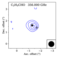
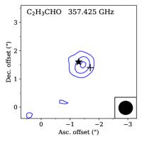
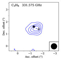
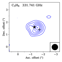
Figure 1: Integrated intensity maps of the line emission for C₃H₆ and C₂H₃CHO, summed over $\pm 0.5$ MHz. The locations of IRAS16293B continuum peak and the offset position are marked by the black star and plus sign, respectively. The blue contours start at 4 $\sigma$ and increase by steps of 4 $\sigma$, where $\sigma$ is 5 mJy beam^-1 km s^-1 for the integrated intensity. A representative beam of 0$\aas@@fstack{\prime\prime}$5 is shown in the lower right corner of each panel.

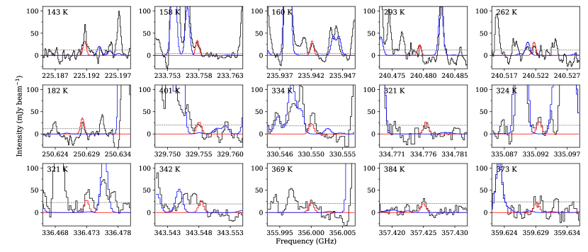
Figure 2: Identified lines of C₂H₃CHO: the synthetic spectrum, in red, is plotted along with the offset position spectrum towards IRAS 16293B. The straight dashed black line represents the detection limit at the intensity of 3$\sigma$. The upper-level energy of the transition is noted in the upper left corner of each panel. The reference spectrum in blue takes the previous species reported in PILS into account (Jørgensen et al. 2016, 2018; Lykke et al. 2017; Coutens et al. 2016; Ligterink et al. 2017; Persson et al. 2018; Calcutt et al. 2018a; Drozdovskaya et al. 2018; Manigand et al. 2019).

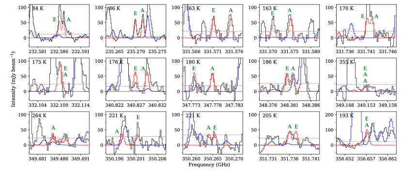
Figure 3: Identified lines of C₃H₆: the synthetic spectrum, in red, is plotted along with the offset position spectrum towards IRAS 16293B. The dashed lines correspond to optically thick lines. The straight dashed black line represents the detection limit at the intensity of 3$\sigma$. The upper-level energy of the transition is noted in the upper left corner of each panel. The torsional state ‘E’ or ‘A’ of each transition is noted in green on the spectra. The reference spectrum in blue takes the previous species reported in PILS into account (see Figure 2 and references therein).

A total of 12 unblended lines of C₂H₃CHO have been identified across Bands 6 and 7, with an intensity higher than 3$\sigma$ – with $\sigma$ calculated as the root mean square (RMS) of the noise spectrum. 38 other lines that match in terms of frequency were found in the range of the observations. However, they show significant blending with other species. All the lines predicted by the local thermodynamic equilibrium (LTE) model are present in the observations. The upper-level energies of the detected transitions lie between 158 and 401 K, which provide constraints on the excitation temperature. Among these transitions, those at frequencies of 225.192, 330.550 and 336.473 GHz have been used in the fit even though they seem to be slightly blended with other species. All these transitions are listed in Table LABEL:app-linelist-C2H3CHO. C₂H₃CHO has been searched for towards IRAS 16293A as well, however, no lines above 3$\sigma$ were found, presumably due to the larger linewidth ($\sim$3 km s^-1), and thus the more severe blending, compared to IRAS 16293B.

For C₃H₆, 21 unblended lines were found in the different frequency ranges of the observations. The upper-level energies of the detected transitions lie between 84 and 264 K. 34 lines above 3$\sigma$ are present in the spectrum, but they are significantly blended with other species, thus they were discarded from the fit. The transition at 349.153 GHz, with an upper-level energy of 355 K, was used in the fit to better assess the excitation temperature, even though the intensity of the line is lower than 3$\sigma$. All these transitions are listed in Table LABEL:app-linelist-C3H6. The same lines were found to be completely blended towards IRAS 16293A.

Figure 1 shows the integrated line emission of C₂H₃CHO and C₃H₆. The spatial extent of their emission is marginally resolved and located in the hot corino region, consistently with the other O-bearing COMs detected in the same dataset (e.g. Jørgensen et al. 2016; Lykke et al. 2017; Calcutt et al. 2018b).

HCCCHO, n-C₃H₇OH and i-C₃H₇OH, as well as C₃O and cis-HC(O)CHO were searched for in the data, however, no line above 1$\sigma$ was found.

3.2 Column densities

Table 2: Column densities of detected species and upper limits of non-detection towards the offset position from IRAS 16293B.

Species	$T_{\mathrm{ex}}$ (K)	$N_{\mathrm{tot}}$ (cm-2)	Ref.
C2H3CHO	$125\pm 25$	$3.4\pm 0.7\times 10^{14}$	1
C3H6	$75\pm 15$	$4.2\pm 0.8\times 10^{16}$	1
HCCCHO	100	$<5.0\times 10^{14}$	1
n-C3H7OH	100	$<3.0\times 10^{15}$	1, 2
i-C3H7OH	100	$<3.0\times 10^{15}$	1, 2
C3O	100	$<2.0\times 10^{13}$	1
cis-HC(O)CHO	100	$<5.0\times 10^{13}$	1
C3H8	100	$<8.0\times 10^{16}$	1
CH3CCH	$100\pm 20$	$1.1\pm 0.2\times 10^{16}$	3
C2H5CHO	$125\pm 25$	$2.2\pm 1.1\times 10^{15}$	4
CH3CHO	$125\pm 25$	$7.0\pm 3.5\times 10^{16}$	4
CH3COCH3	$125\pm 25$	$1.7\pm 0.8\times 10^{16}$	4
C2H5OCH3	$100\pm 20$	$1.8\pm 0.2\times 10^{16}$	5

(1) this work; (2) Qasim et al. (2019); (3) Calcutt et al. (2019); (4) Lykke et al. (2017); (5) Manigand et al. (2020).

The identification of C₂H₃CHO and C₃H₆ has been confirmed by modelling the molecular emission under the LTE assumption and comparing the spectrum extracted at an offset position from the continuum peak position of IRAS 16293B. The model has been used in Manigand et al. (2020), where more substantial details can be found. This synthetic spectrum considers the gas as a homogeneous slab under LTE conditions and uses the optically thin molecular lines to fit the observed spectrum and to estimate the column density, the rotational temperature, the peak velocity shift, the FWHM and the source size, which is fixed to 0$\aas@@fstack{\prime\prime}$5, based on the previous PILS studies.

We run a grid of models in column densities from 10¹³ to 10¹⁷ cm^-2 and for excitation temperatures ranging from 50 to 300 K in steps of 25 K. The peak velocity shift and FWHM were set to 2.7 and 0.8 km s^-1, respectively, for C₂H₃CHO and 2.5 and 0.8 km s^-1, respectively, for C₃H₆, after a visual inspection of the alignment of the observed lines and the model. The best model was estimated through a $\chi^{2}$ minimisation, with a modified weighting factor as detailed in Manigand et al. (2020). The modified weighting factor favours the under-estimation of the intensity of the modelled spectrum, which reflects possible unexpected blending effects with other species. A correction factor was applied to the derived column density to take into account the continuum contribution as detailed, for example, in Jørgensen et al. (2018) and Calcutt et al. (2018b). The relative uncertainty of the column density and the rotational temperature is 20%.

The best agreement between the data and the model for C₂H₃CHO was found at an excitation temperature of $125\pm 25$ K and a column density of $3.4\pm 0.7\times 10^{14}$ cm^-2. All the lines used in the fit are shown in Figure 2. The lower intensity of the lines in Band 7 compared to those in Band 6 emphasises the relatively low rotational temperature derived from the model.

Figure 4: Identified lines of C₃H₆ synthetic spectrum, in red, including the E/A spin weight ratio of $0.6\pm 0.1$ are plotted along with the offset position spectrum towards IRAS 16293B. The dashed lines correspond to optically thick lines. The straight dashed black line represents the detection limit at the intensity of 3$\sigma$. The upper-level energy of the transition is noted in the upper left corner of each panel. The torsional state ‘E’ or ‘A’ of each transition is noted in green on the spectra. The reference spectrum in blue takes into account the previous species reported in PILS (see Figure 2 and reference therein).

The rotational temperature and column density of C₃H₆ was found to be $75\pm 15$ K and $4.2\pm 0.8\times 10^{16}$ cm^-2, respectively. All the brightest lines in Band 6 are marginally optically thick for the best fit physical conditions. Nevertheless, the optically thick line at 235.272 GHz shows very good agreement with the observed line, which consolidates the unusually low value of 75 K found for the rotational temperature towards the IRAS 16293B hot corino region. The C₃H₆ lines used to assess the column density and the rotational temperature are shown in Figure 3.

The majority of C₃H₆ transitions are split into A and E torsional sub-states due to the CH₃– group in the molecule. This kind of split is common to most of the species having the CH₃ group, such as CH₃OH or CH₃OCHO. For C₃H₆, the intensities of the lines at 340.827, 347.774 and 351.738 GHz, corresponding to E-transitions, are overestimated by the LTE model. The A-transitions that have the same quantum numbers, in particular the same upper-level energies and Einstein’s coefficients, are in good agreement with the model. This overestimation of the E-transitions alone may suggest that the spin weight ratio between the transitions arising from A and E substates is not equal to unity.

To test this hypothesis, we added the spin weight of the E-transitions with respect to the A-transitions in the LTE model and assessed this ratio, given the best fit found for the excitation temperature, velocity shift and FWHM. This spin weight factor $g_{\text{E/A}}$ is multiplied to the upper state degeneracy of the E-transitions. The best fit was found at the same column density, i.e. $4.2\pm 0.8\times 10^{16}$ cm^-2, and a spin weight ratio of $g_{\text{E/A}}=0.6\pm 0.1$. Figure 4 shows the LTE model, including the discrepancy of the E-transitions with respect to the A-transitions. This difference between the A- and E-transitions could reflect an abundance asymmetry between the different conformers, due to low temperature at the moment of their formation, for example. Similar E/A ratios were observed towards dark clouds (Friberg et al. 1988), cold prestellar clumps (Menten et al. 1988) and more recently towards young stellar objects (Wirström et al. 2011). Nevertheless, in this study, there are still too few isolated transitions to be able to rule out any bias from the spectroscopic data that could explain this asymmetric E/A spin ratio.

For the sake of the chemical modelling comparison, the upper limits on the column density were derived for HCCCHO, C₃H₇OH, C₃O, C₃H₈, and cis-HC(O)CHO. These upper limits correspond to the column density reached in the model when the most intense lines reached 3$\sigma$ at $\sim$100 K, which is the average excitation temperature of C₂H₃CHO and C₃H₆. The upper limit of cis-HC(O)CHO leads to an upper limit of the total amount of HC(O)CHO of $<$ 2.6 $\times\leavevmode\nobreak\ 10^{23}$ cm^-2 in the gas phase, which does not provide any real constraint on this molecule. Table 2 summarises the column densities and rotational temperatures of the newly detected species towards source B. Previous detections of chemically related species, namely acetaldehyde (CH₃CHO), acetone (CH₃COCH₃), ethyl methyl ether (C₂H₅OCH₃), C₂H₅CHO and CH₃CCH, reported from the same dataset by Lykke et al. (2017) and Calcutt et al. (2019), are also indicated in the table and have been used for a comparison with the chemical model. Qasim et al. (2019) already reported a column density upper limit for Ga-n-C₃H₇OH of $<1.2\times 10^{15}$ cm^-2 at 300 K and $<7.4\times 10^{14}$ cm^-2 at 125 K, using the Band 6 dataset of Taquet et al. (2018). Given their same dataset and the correction factor to include the contribution of the other conformers, this estimate is consistent with the results presented here. In the following, we consider the more conservative column density upper limit of $<3.0\times 10^{15}$ cm^-2.

4 The chemical model

In this section, we compare the abundance, and the upper limits, derived from the observations towards IRAS 16293B with a physico-chemical model of a typical low-mass forming star. The core of the simulation uses the Nautilus code (Ruaud et al. 2016), a 3-phase (gas, dust ice surfaces and dust ice mantle) time-dependent chemical model. The chemical study presented here is very similar, in terms of realisation, chemical code and astronomical source, to the studies of Andron et al. (2018) and Coutens et al. (2019). The majority of the differences resides in the extended chemical network used here.

The following subsections present the physical model that describes the evolution of physical conditions of the dust and gas during the simulation, the chemical network that computes the abundance variation caused by the reactions included in the network and the results obtained from the simulations.

4.1 Physical model

Two successive evolutionary stages of a low-mass protostar are simulated: a uniform and constant stage, corresponding to the pre-stellar phase, or the cold-core phase, followed by an evolving stage during which the density and the temperature at the centre of the cloud increases while the envelope is collapsing towards the centre until breaking the hydrostatic equilibrium to form the protostar, i.e. the collapse phase.

The cold-core phase consists of a homogeneous and static cloud at a temperature of 10 K for both gas and dust, a gas density of $2\times 10^{4}$ cm^-3, a visual extinction of 4.5 mag, a cosmic-ray ionisation rate of $1.3\times 10^{-17}$ s^-1, and a standard external UV field of 1 G₀. The collapse phase is the same as used by Aikawa et al. (2008, 2012), Wakelam et al. (2014), Andron et al. (2018), and Coutens et al. (2019). The physical structure used in their study was derived from a 1D radiative hydrodynamical model (Masunaga & Inutsuka 2000), starting from the infall of the cold core, until the collapse stage of the first hydrostatic core, triggered by the dissociation of H₂ by collisions. While the physical structure evolves with time, several parcels of gas are tracked in time and position and their physical properties are traced throughout the collapse. Each parcel ends up at a different radius at the end of the simulation, which allows the evolution of the distribution of the molecular compounds included in the chemical network to be followed. In this study, the chosen parcel of gas starts the collapse at a radius of ¿ $10^{4}$ au, where it stays for the major part of the collapse and ends-up at a radius of 15 au (see Figure 5 in Aikawa et al. 2008), where the gas reaches a temperature of $\sim 265$ K and a density of $4\times 10^{8}$ cm^-3. Figure 7 shows the evolution of the physical conditions of the targeted parcel of dust and gas. The parcel spends only the last couple of hundred years at a temperature higher than 100 K at a radius ¡$130$ au.

4.2 Chemical network

The chemical network includes the kida.uva.2014 gas-grain-phases network as a base (Wakelam et al. (2012, 2015) with updates from Ruaud et al. (2015); Hincelin et al. (2015); Loison et al. (2016); Hickson et al. (2015, 2016a); Wakelam et al. (2017); Loison et al. (2017); Vidal et al. (2017)). The initial abundances used in the simulations are listed in Table 3.

Table 3: Initial abundances used in the chemical model.

Species	n / n(H)	Species	n / n(H)
H2	$5.0\times 10^{-1}$	S+	$1.5\times 10^{-6}$
He	$9.0\times 10^{-2}$	Fe+	$1.0\times 10^{-8}$
O	$2.4\times 10^{-4}$	F	$6.68\times 10^{-9}$
C+	$1.7\times 10^{-4}$	Cl+	$1.0\times 10^{-9}$
N	$6.2\times 10^{-5}$

Despite the inclusion of dozens of new species, hundred of new reactions, and the inclusion of hundreds of theoretical calculations to determine reaction barriers, there are still large uncertainties on branching ratios due to the lack of experimental studies and the difficulty of determining these branching ratios theoretically. Besides, the diffusion energies of radicals on surfaces are not well-known, which again leads to great uncertainties in determining which reactions becomes the most important when the temperature rises. More details on the upgrades made to the chemical network can be found in Appendix B.1.

The chemical model distinguishes the ice surface and the ice mantle during the computation of the chemical reactions and the interaction processes between the different phases. For the comparison with the observations, the ice surface and ice mantle are considered as a single phase. We consequently summed the ice surface and ice mantle abundances to get the total ice abundances. The species in the solid phase are annotated with ‘s-’ in front of their names.

To discuss the formation and destruction paths of the different species, the abundances relative to H₂ have been used in the comparison. This representation is convenient for discussing the evolution of the abundances with the modification of the density and the temperature along with the collapse of the protostellar envelope. The H₂ column density can be derived from the dust continuum radiation, assuming a dust size and an opacity distributions. However, the high continuum absorption seen towards IRAS 16293B in the PILS observations suggests that the dust emission is optically thick. Jørgensen et al. (2016) estimated the lower limit of $>$1.2 $\times$ 10²⁵ cm^-2 for the H₂ column density. Therefore, we chose to use the abundances relative to CH₃OH when comparing the final state of the simulation to the observational results. The abundances derived from the observations are taken from Jørgensen et al. (2016, 2018); Lykke et al. (2017); Manigand et al. (2020) and this study.

4.3 Simulation runs

Different reactions have been considered to reproduce the observations similarly to what has been done in other studies (e.g. Coutens et al. 2018a). Among the important reactions investigated in this paper, the gas-phase formation reaction involving OH is crucial in the formation of C₃O from the consumption of C₃ and has been studied by Loison et al. (2017):

$$\mathrm{OH+C_{3}}\longrightarrow\mathrm{C_{3}O+H}$$ (1)

The surface production pathways are marginally contributing to the formation of C₃O radicals present on the ice surfaces, during the pre-stellar phase. The major destructive path of C₃ occurs through the gas-phase reaction:

$$\mathrm{O+C_{3}}\longrightarrow\mathrm{C_{2}+CO}$$ (2)

This reaction is thought to play an important role in the abundance of C₃H_x, C₃O, and C₂H_xCHO species (Hickson et al. 2015). The radical-radical addition reactions on grain surfaces are marginally contributing to the final abundances of these complex species.

To investigate the chemical network involved in the formation of C₃-species, we run several simulations, depending on the tested chemical branch:

• A1: This simulation is the fiducial model, with which the other models can be compared. The common COMs, such as CH₃OCH₃ and CH₃OCHO, are mainly formed on grain surfaces but gas-phase formation pathways are also included, except for CH₂(OH)CHO, (CH₂OH)₂ and CH₃OCH₂OH. The hydroxyl radical OH contributes only to the formation of C₃O and HCCCHO in the gas phase. A reaction rate of $1.0\times 10^{-12}$ cm³ molecule^-1 s^-1 is considered for the gas-phase reaction (2).

• B1: The hydrogenation of HC(O)CHO, based on Chuang et al. (2016), has been added to the grain surface reaction network:

  $$\mathrm{\text{s-}HC(O)CHO+2\ \text{s-}H} \longrightarrow \mathrm{\text{s-}CH_{2}(OH)CHO}$$ (3)

  $$\mathrm{\text{s-}CH_{2}(OH)CHO+2\ \text{s-}H} \longrightarrow \mathrm{\text{s-}(CH_{2}OH)_{2}}$$ (4)

  In addition, we have included the hydrogenation of CH₃OCHO, forming CH₃OCH₂OH, to the network:

  $$\mathrm{\text{s-}CH_{3}OCHO+2\ \text{s-}H}\quad\longrightarrow\quad\mathrm{\text{s-}CH_{3}OCH_{2}OH}$$ (5)

  based on the hydrogenation of CH₂(OH)CHO (reaction 3).

• C1: This run uses the same reaction network as the fiducial run A1. In this case, the pre-stellar phase lasts longer than the other runs, i.e. $3\times 10^{6}$ yr instead of $1\times 10^{6}$ yr, which gives the cold chemistry more time to proceed.

• D1: In order to evaluate the contribution rate of the radical-radical addition on the grain surface to the abundance of HCCCHO, C₂H₃CHO and C₂H₅CHO, the following reactions have been removed from the network:
  

  $$\mathrm{\text{s-}HCO}+\mathrm{\text{s-}C_{2}H_{3}} \longrightarrow \mathrm{\text{s-}C_{2}H_{3}CHO}$$ (6)

  $$\longrightarrow \mathrm{\text{s-}C_{2}H_{4}+\text{s-}CO}$$ (7)

  $$\mathrm{\text{s-}HCO}+\mathrm{\text{s-}C_{2}H_{5}} \longrightarrow \mathrm{\text{s-}C_{2}H_{5}CHO}$$ (8)

  $$\longrightarrow \mathrm{\text{s-}C_{2}H_{6}+\text{s-}CO}$$ (9)

  The addition reaction of HCO and C₂H on grains is not contributing to the formation of HCCCHO in our chemical network because the amount of available C₂H on the ice surfaces is limited by the very high activation barrier of the hydrogen abstraction of C₂H₂ (¿56 000 K, Zhou et al. 2008).

• E1: This run takes into account the hydrogenation of HC(O)CHO and CH₃OCHO, as it is for run B1, and the activation energies for hydrogenation and abstraction reactions of H₂CO, CH₃OH, C₂H₂, C₂H₄, C₂H₆, C₂H₃CHO, and C₂H₅CHO, taken from the recent laboratory study of Qasim et al. (2019) about propanal and propanol formation on ice surfaces from CO, and the references therein (Andersson et al. 2011; Goumans & Kästner 2011; Kobayashi et al. 2017; Song & Kästner 2017; Álvarez-Barcia et al. 2018; Zaverkin et al. 2018). The activation energies taken from Qasim et al. (2019) are, in general, lower than those used in the simulation runs A1 to D1.

• A2 to E2: These runs are similar to the runs A1 to E1, but with a lower reaction rate of $10^{-16}$ cm³ s^-1 for reaction (2).

The list of the reactions added, extrapolated or removed in each run, with the associated branching ratios and reaction rates, is presented in Appendix B.2. The formation enthalpies of the intermediate species that intervene in the new hydrogenation paths on grain surfaces are taken from Goldsmith et al. (2012).

4.4 Modelling results

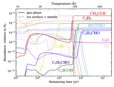
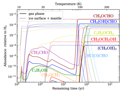
Figure 5: Time evolution of abundances in the gas phase (solid lines) and on the grain surface (dotted) of several species during the collapse phase of the A1 run. The time axis is reversed to better visualise the abundances evolution. Both panels show the results of the same simulation but with a different selection of species, with their name annotated following the colour code of the curves.

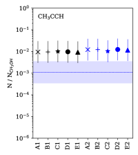
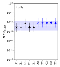
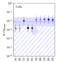
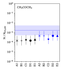
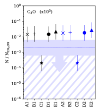
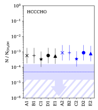
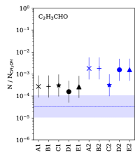
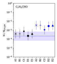
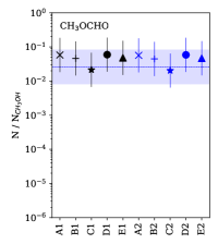
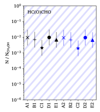
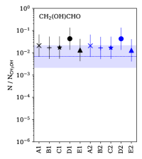
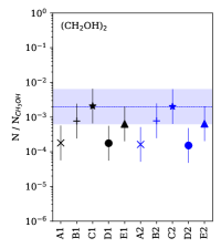
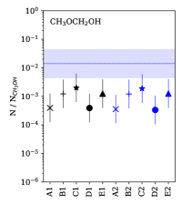
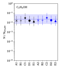
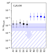
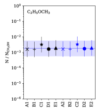
Figure 6: Final abundances reached at the end of each simulation run for the targeted species. The dashed blue line shows the observed abundance of the species towards IRAS 16293B. The error bars and the blue area correspond to one half order of magnitude confidence limit, thus a 1$\sigma$-difference between observations and simulations corresponds to one order of magnitude. The dashed blue region represents the abundance values that are consistent with the corresponding upper limit. The abundance scale of C₃O is lower than the other plots. The abundance upper limit of HC(O)CHO is $<$ 2.6 $\times 10^{4}$ relative to CH₃OH, therefore, there is no observational constraint on the abundance of HC(O)CHO. The abundance upper limit of C₃H₇OH is the sum of n-C₃H₇OH and i-C₃H₇OH abundance upper limits.

The evolution of the abundances during the collapse phase of the run A1 is shown in Figure 5. For the COMs formed in a hot corino region, most of the molecules targeted are produced on grain surfaces and are released in the gas-phase when the temperature reaches the desorption temperature, between 80 to 130 K depending on the species.

This production scheme leads to a jump of several orders of magnitude in gas-phase abundances of the species around such temperatures. Concerning the C₃-species, the jump in gas-phase abundances is smaller which indicates significant gas-phase production route contributions. These gas-phase contributions seem higher for the most unsaturated species, such as HCCCHO, C₃ and C₃O. At the end of the simulation, all the formed molecules are in the gas phase.

Figure 6 summarises the gas-phase abundances relative to CH₃OH of the C₃-species that are under investigation in this study and a few other COMs, such as CH₃OCHO, CH₂(OH)CHO, (CH₂OH)₂, CH₃OCH₂OH, C₂H₅OH, CH₃COCH₃, and C₂H₅OCH₃, at the end of the collapse phase for every simulation. Because of the assumptions from the physical model compared to the actual physical structure of IRAS 16293B, which is still not perfectly known, an abundance difference of less than one order of magnitude is considered as an agreement between the simulation and the observations.

4.4.1 C₃-species

The abundances of C₃–species, that are CH₃CCH, C₃H₆, C₃H₈, HCCCHO, C₂H₃CHO, and C₂H₅CHO, are correlated to those of their precursors, C₃ and C₃O. As C₃ is efficiently produced and is not a very reactive species in the gas phase, s-CH₃CCH and s-C₃H₆ are quite abundant in the solid phase. The comparison between the runs A1–E1 and A2–E2 shows that most of the C₃-species are sensitive to a decrease in the reaction rate of the C₃ destruction reaction (2). As the reaction rate decreases, there is more C₃ available to form C₃-species, thus their abundances increase. The increase in the abundances is more pronounced for the more saturated species.

The abundances of the C₃-species at the end of the simulation run C1 are significantly different from those at the end of the fiducial run. The longer time spent at very low temperatures during the prestellar phase pushes the hydrogenation reactions to produce more saturated C₃-species by consuming the unsaturated precursors. This is particularly shown by the lower abundances of C₃O and HCCCHO contrasting the higher abundances of C₂H₃CHO and C₂H₅CHO.

The ice-surface formation pathways of C₂H₃CHO and C₂H₅CHO, through reactions (6) and (8), are deactivated in the simulation run D1. The final abundances show a decrease compared to the simulation where the molecules are produced through ice-surface reactions, among others. The updated activation energies, taken from the study of Qasim et al. (2019) and tested in the simulation E1, do not change the final abundances of the C₃-species significantly.

The C₃H₇OH species is a particular case as there is an alternative production pathway apart from successive hydrogenation of C₃O, mostly the O + C₃H₈ reaction. The slight overestimate for C₃H₇OH may be due to an overestimate of the s-OH + s-C₃H₇ recombination branching ratio versus the disproportionation, that is the exchange reaction of one H atom from one radical to the other:

$$\text{s-OH}+\text{s-}\mathrm{C_{3}H_{7}}\longrightarrow\text{s-}\mathrm{H_{2}O}+\text{s-}\mathrm{C_{3}H_{6}}$$ (10)

Its isomer C₂H₅OCH₃, however, is well reproduced by the models, despite the fact that there is only the formation pathway through radical-radical addition that are implemented in the chemical network (see Table 4 in Appendix). The variation of the final abundance of C₂H₅OCH₃ is very similar to that of C₂H₅OH which suggests that they share the same type of formation reactions on ice surfaces, assuming that the major formation pathways of C₂H₅OH effectively take place on ice surfaces as well.

4.4.2 COMs hydrogenation

Concerning the species formed through radical-radical addition, the slight to large overestimation or underestimation of the calculated abundances when considering the fiducial run A1 likely reflects the uncertainties of the association channel branching ratios compared to the disproportionation channel.

The underestimation of (CH₂OH)₂ is unexpected considering the large amount of s-CH₂OH as well as the large branching ratio used for the reaction s-CH₂OH + s-CH₂OH $\rightarrow$ s-(CH₂OH)₂, that is 50%, in the fiducial chemical network. Despite the approximate agreement between the simulations and the observations for CH₃OCHO and CH₂(OH)CHO, these two species are over-produced by the radical-radical additions whereas (CH₂OH)₂ and CH₃OCH₂OH, which are only produced by radical-radical additions on grain surfaces, are both under-produced.

The run B1 includes the hydrogenation formation pathways on grain surfaces of HC(O)CHO and CH₃OCHO. These reactions lead to the consumption of the unsaturated species and the production of saturated ones. The agreement of this run with observations is better than for the fiducial chemical network in terms of abundances of CH₂(OH)CHO, (CH₂OH)₂, CH₃OCHO, and CH₃OCH₂OH, suggesting that hydrogenation reactions play an important role in formation of such COMs in hot corino regions. The hydrogenation of CH₃OCHO has been recently studied in laboratory by Krim et al. (2018). They reported a calculated energy barrier of 32.7 kJ mol^-1 for the ice-surface reaction s-H + s-CH₃OCHO and concluded that this pathway did not seem to contribute to the formation of CH₃OCH₂OH. The experimental result of Krim et al. mainly shows that this reaction is slower than the s-H + s-H₂CO $\rightarrow$ s-CH₃O reaction but does not completely exclude its role in interstellar ice conditions. In our simulation, we include this reaction with a barrier equal to 3000 K (25 kJ mol^-1) as average between the value calculated in this work, the value calculated by Krim et al., and the value calculated by Álvarez-Barcia et al. (2018), i.e. 4960 K (41.2 kJ mol^-1). This reaction, like all H reactions with barriers, is partly allowed by the tunnel effect.

The reaction s-HCO + s-HCO has been suggested to produce s-HC(O)CHO (Fedoseev et al. 2015; Chuang et al. 2016) to explain the formation of CH₂(OH)CHO and (CH₂OH)₂ in experimental surface hydrogenation of CO molecules. HC(O)CHO production through s-HCO + s-HCO reaction is also achieved by Simons et al. (2020) using density functional theory (DFT, Scuseria & Staroverov 2005) calculations in a model in which the surface molecules were not explicitly taken into account. Additionally, the recent experimental work of Butscher et al. (2017) indicates that the reaction of two HCO radicals on ice surfaces does not lead to HC(O)CHO but rather to H₂CO and CO. Considering the conflicting results from different studies, it is difficult to estimate the proportion of HC(O)CHO produced by the s-HCO + s-HCO reaction. In this study, we consider a branching ratio of 5% for HC(O)CHO formation through the s-HCO + s-HCO reaction. This leads to a significant production of HC(O)CHO due to the great abundance of HCO on the grains, which is around 1% of the CH₃OH (see Figure 6). The comparison with the observations is delicate because the most stable isomer of HC(O)CHO, the trans- one, has no dipole moment and the population fraction of cis-HC(O)CHO is equal to $1.9\times 10^{-10}$ at 100 K, considering that the thermal equilibrium is reached, and is not detected in the observations.

The updated activation energies from Qasim et al. (2019) of abstraction reactions of CH₃OH and H₂CO affect the final abundances of the COMs that are predominantly formed through radical-radical addition reactions. In particular, the lower final abundance of (CH₂OH)₂ in run E1 compared to B1 is affected by the newly implemented abstraction reaction of CH₃OH which produces CH₃O radicals.

5 Discussion

In most of the models, C₃ reaches a high abundance in the gas phase, due to its low reactivity. This leads to a high abundance of s-C₃ in solid phase, which results in high abundances of all the C₃-species in the gas phase, especially CH₃CCH, C₃O, and HCCCHO, which are much more abundant than observed. A better agreement to the observations can be found when the rate constant for the $\mathrm{O+C_{3}}\longrightarrow\mathrm{C_{2}+CO}$ gas-phase reaction is set to $1\times 10^{-12}$ cm³ s^-1, assuming a lower activation barrier than in the theoretical work of Woon & Herbst (1996).

The agreement for CH₃CCH, C₃H₆, C₂H₃CHO, and C₂H₅CHO is rather good between the fiducial run A1 and the observations for IRAS 16293. However, this leads to an underestimation of CH₃CCH and C₃H₆ abundances in the case of dense molecular clouds, the agreement being notably less good with observations of TMC-1 (Marcelino et al. 2007; Markwick et al. 2002) as shown by Hickson et al. (2016b). Alternatively, the abundances of C₃O and HCCCHO are in good agreement with the observations for dense clouds (Herbst et al. 1984; Irvine et al. 1988; Ohishi & Kaifu 1998; Loison et al. 2016), but they are overproduced for IRAS 16293B. The overproduction of C₃O and HCCCHO for the case of IRAS 16293B may be due to under-represented consumption pathways of these species through ice-surface reactions and demonstrates that laboratory studies in this area are required.

The duration of the prestellar phase has a significant impact on the COM abundances at the end of the simulation. A longer time spent in the prestellar phase enhances the impact of efficient reactions at cold temperature (10 K) on the final abundance. This effect is presumably due to the ongoing hydrogenation at cold temperature, and the addition of nearby radicals, with a non-efficient thermal diffusion on the ice surfaces at a such temperature. The agreement with the observations for C₃H₆ and C₃H₈ is particularly better with a longer prestellar phase in the simulation. The impact on the abundance of C₂H₃CHO and C₂H₅CHO is less important in comparison with the observations.

Concerning the other COMs, a longer prestellar phase leads to a better match of the simulated and observed abundances, in particular for (CH₂OH)₂. The absence of strong outflows from IRAS 16293 B has been suggested as due to this protostar being the less evolved source compared to its companion (van der Wiel et al. 2019), which shows at least two major outflows (Yeh et al. 2008; Kristensen et al. 2013; Girart et al. 2014). The abundance ratio of vinyl cyanide (C₂H₃CN) and ethyl cyanide (C₂H₅CN) observed by Calcutt et al. (2018b) suggests that the warm-up timescale was shorter for IRAS 16293A, the more luminous binary component, or it has a higher accretion rate compared to IRAS 16293B. Another scenario could be that IRAS 16293A started to collapse earlier than IRAS 16293B. This delay of the beginning of the collapse of each protostar of a binary system could be the result of the fragmentation of the parent cloud when the first protostar started to form. This scenario is in agreement with the dynamical modelling study of Kuffmeier et al. (2019), in which the CO-rich bridge structure between the two protostars has been interpreted as a product of the multiple system dynamics and could be a remnant of the parent cloud fragmentation.

The agreement with the observations of the abundance ratios of unsaturated species over saturated ones between the three C₂H_xCHO species is associated with an overall overproduction of these species during the prestellar phase. This overproduction suggests that the common precursors C₃, and then C₃O, are also overproduced. The over-abundance of C₃ and C₃O could be a result of an underestimation of the consumption of these species by a lack of reactions in the chemical network. The largest carbon-chain species taken into account in the chemical network are C₅H_x in linear forms, and a few benzene-like molecules, such as C₆H₅CN, associated to their recent detection in the ISM reported in the study of McGuire et al. (2018). The larger poly-aromatic hydrocarbons (PAH), which are expected to be abundant in space (Puget & Leger 1989), are not included in the calculation. This limitation in the size of carbon-chain species might be the origin of the over-production, or underconsumption, of the small carbon-chain species, which are the building blocks of these PAHs at cold temperatures as suggested by the recent studies of Joblin & Cernicharo (2018) and Kaiser et al. (2015).

6 Conclusion

This study presents the observations and the chemical modelling of C₃-species around the Class 0 protostar IRAS 16293B. Using ALMA observations from the PILS survey, the molecular emission is analysed by comparing the spectrum to LTE models to determine the excitation temperatures and column densities of these species. Then, the abundances relative to CH₃OH are compared to the three-phase chemical model Nautilus to investigate the different formation pathways of such molecules under the typical physical conditions of the hot corino region. Different models were tested, each one focusing on a single aspect of the chemical network. The key findings are summarised in the following:

1. We report the first detection of C₂H₃CHO and C₃H₆ towards the protostar IRAS 16293B. Their emission has an excitation temperature of 125 and 75 K, respectively, and their column densities are found to be $3.4\pm 0.7\times 10^{14}$ and $4.2\pm 0.8\times 10^{16}$ cm^-2, respectively. These molecules were not detected towards the other member of the binary system. For C₃H₆, the E-transitions were found to exhibit a lower intensity with respect to the A-transitions, leading to a ratio of the E-transitions over A-transitions emitting molecules, being $0.6\pm 0.1$ in terms of column densities. The column density upper limits of several chemically related species, that are HCCCHO, C₃H₇OH, C₃O, HC(O)CHO, and C₃H₈, are also reported to provide constraints on the chemical simulations.

2. Most of the simulations reproduce the abundances observed towards IRAS 16293B within an order of magnitude. The final abundances of the different simulations are sensitive to the duration of the prestellar phase, especially when the successive hydrogenation reactions play an important role in the formation of more saturated species. This seems to be the case for CH₃CCH, HC(O)CHO and CH₃OCHO which form C₃H₆, C₃H₈, CH₂(OH)CHO, (CH₂OH)₂ and CH₃OCH₂OH. The longer the cloud spends at low temperatures, the more abundant the saturated species, and the more depleted the precursors.

3. On ice surfaces, the successive hydrogenation reactions of C₃O, forming HCCCHO, C₂H₃CHO, and C₂H₅CHO, and the radical-radical additions of HCO and C₂H₃ or C₂H₅ equally contribute to the amount of C₃-species observed in the hot corino of IRAS 16293B.

4. A high gas-phase reaction rate of $1\times 10^{-12}$ cm³ s^-1 for the gas-phase reaction $\mathrm{C_{3}+O}\rightarrow\mathrm{C_{2}+CO}$ is necessary to fit the final abundances of C₃-species detected in the observations. The very efficient production of C₃ and C₃O, along with the overall overproduction of C₃-species, suggests that consumption pathways of C₃ species are missing in the chemical network. These chemical routes could be related to the production and growth of PAHs at cold temperatures, which are not included in the present chemical model.

Most of the models reproduce the abundances of the C₃-species towards IRAS 16293B, which emphasises the contribution of the grain-surfaces production pathways under the hot corino physical conditions. Besides, the formation of these species on grain surfaces suggests that they can be incorporated into the protostellar disk as the protostar evolves into a Class I protostar and contribute to the formation of prebiotic molecules. Deeper observations of Class I protostellar disks and the detection of more complex species towards Class I objects are necessary to clearly state on the presence of these molecular species in such objects. Finally, the overproduction of unsaturated C₃-species, in general, suggests the lack of longer carbon-chain molecules formation pathways on grain surfaces and in gas phase and indicate the need of laboratory and theoretical studies of such reactions.

Appendix A Physical model evolution

Figure 7 shows the evolution of the density, the temperature, the extinction coefficient and the infall velocity of the gas during the collapse phase.

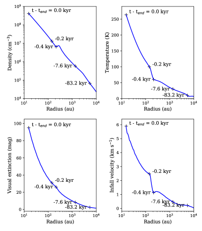
Figure 7: Evolution of the density, dust temperature, visual extinction and infall velocity across the envelope during the simulation. The time is indicated at several positions on the curves, with $t=0$ yr set to the end of the collapse phase in the simulation.

Appendix B Chemical network

B.1 Upgrades from the NAUTILUS public version

The chemical network used here is limited to a skeleton up to five atoms of carbons for linear chains, including oxygen nitrogen and sulfur-bearing, neutral and ionic compounds. Besides, benzene, benzonitrile (C₆H₅CN) and ethylbenzene (C₆H₅C₂H) are also included with their ions. Special care has been taken with end-of-chain processing, which is an important source of error for finite models that want to account for infinite chemistry. In principle, there is no limit for the formation of very large molecules, that are then associated to a very large dilution and thus an abundance of large molecules in most cases very small by bottom-up chemistry. In other words, the limitations are imposed by the extent of the chemical network and the formation of molecules up to five carbons in their structure ensures a proper representation of the production of smaller molecules, such as the C₃-species. Even though there are some notable changes in the gas-phase chemistry (new reactions, update of rate constants and branching ratios according to new measurements and theoretical calculations), the most important changes were made for the grain-surfaces chemistry. The chemistry will be detailed in future articles, thus we only present major changes that concern the species discussed in this work.

We have started to homogenise the chemistry on grains completing the possible reactions for the most abundant species on grains. First, we systematically supplemented the hydrogenation reactions through s-H and s-H₂ reactions, which are critical because they are favoured by the completion between diffusion and reaction through tunnelling. To estimate the probabilities of the tunnelling effect, we systematically consider a barrier width of 1 Angstrom and we calculate the height of the reaction barriers in the gas phase using the density functional theory (DFT, Scuseria & Staroverov 2005) with the functional M06-2X and the AVTZ basis (Zhao & Truhlar 2008); we have calculated 240 barrier heights for s-H and s-H₂ reactions. The reactions with s-H₂ lead to quick consumption of s-CN, s-OH, s-NH₂, s-C, s-CH, s-CH₂, s-C₂, s-C₂H, s-C₂H₃ as long as there is a lot of s-H₂ on grains. Reactions of these species with s-H₂ are exothermic and are enhanced by tunnelling effect when an activation barrier exists. For some low exothermic reactions, such as s-CH₂ + s-H₂, s-C₂H₃ + s-H₂, and s-NH₂ + s-H₂, a barrier of 1 Angstrom undoubtedly overestimates the tunnelling effect. However, considering the very high abundance of s-H₂, this should not be critical in the end, at least as long as there is a lot of s-H₂ on grains, although more accurate tunnelling treatment would be desirable in the future. We have also modified the Nautilus code to better take into account the tunnelling effect for reactions involving hydrogen atom transfer between heavy species. For example, the $\mathrm{O+C_{3}H_{8}\rightarrow OH+C_{3}H_{7}\rightarrow C_{3}H_{7}OH\ /\ C_{3}H_{6}+H_{2}O}$ reaction is now an efficient source of propanol production through tunnelling of the first step followed by reaction between s-OH and s-C₃H₇ radicals which are supposed to stay close enough on the grains to react. We also consider diffusion by tunneling for all species, with a diffusion barrier width of 2.5 Angstrom according to Ásgeirsson et al. (2017) and a diffusion barrier height equal to 0.6 of the binding energy. The width of the diffusion barrier is not critical as long as it is greater than 2 Angstrom but limits the reactivity through tunnelling for reactions with a high barrier ($>$ 5000 K).

Table 4: Branching ratios of radical addition reactions.

Reacting species	$\rightarrow\$ Produced species	BR	E${}_{\text{a}}$
		(%)	(K)
s-CH3 + s-CH3	$\rightarrow\$ s-C2H6	100	0
s-CH3 + s-C2H3	$\rightarrow\$ s-C3H6	100	0
	$\rightarrow\$ s-CH4 + s-C2H2	0	0
s-CH3 + s-C2H5	$\rightarrow\$ s-C3H8	100	0
	$\rightarrow\$ s-CH4 + s-C2H4	0	0
s-CH3 + s-HCO	$\rightarrow\$ s-CH3CHO	30	0
	$\rightarrow\$ s-CH4 + s-CO	70	0
s-CH3 + s-CH3O	$\rightarrow\$ s-CH3OCH3	50	0
	$\rightarrow\$ s-CH4 + s-H2CO	50	0
s-CH3 + s-CH2OH	$\rightarrow\$ s-C2H5OH	30	0
	$\rightarrow\$ s-CH4 + s-H2CO	70	0
s-HCO + s-C2H3	$\rightarrow\$ s-C2H3CHO	10	0
	$\rightarrow\$ s-C2H4 + s-CO	90	0
	$\rightarrow\$ s-C2H2 + s-H2CO	0	0
s-HCO + s-C2H5	$\rightarrow\$ s-C2H5CHO	10	0
	$\rightarrow\$ s-C2H6 + s-CO	90	0
	$\rightarrow\$ s-C2H4 + s-H2CO	0	0
s-HCO + s-HCO	$\rightarrow\$ s-HC(O)CHO	5	0
	$\rightarrow\$ s-CO + s-H2CO	95	0
s-HCO + s-CH3O	$\rightarrow\$ s-CH3OCHO	50	0
	$\rightarrow\$ s-CO + s-CH3OH	50	0
	$\rightarrow\$ s-H2CO + s-H2CO	0	0
s-HCO + s-H2CO	$\rightarrow\$ s-CH2(OH)CHO	5	0
	$\rightarrow\$ s-CO + s-CH3OH	95	0
	$\rightarrow\$ s-H2CO + s-H2CO	0	0
s-CH3O + s-CH3O	$\rightarrow\$ s-CH3OOCH3	50	0
	$\rightarrow\$ s-CH3OH + s-H2CO	50	0
s-CH3O + s-CH2OH	$\rightarrow\$ s-CH3OCH2OH	50	0
	$\rightarrow\$ s-CH3OH + s-H2CO	50	0
s-CH2OH + s-CH2OH	$\rightarrow\$ s-(CH2OH)2	50	0
	$\rightarrow\$ s-CH3OH + s-H2CO	50	0
s-O + s-C2H6	$\rightarrow\$ s-C2H5OH	50	2400
	$\rightarrow\$ s-H2O + s-C2H4	50	2400
s-O + s-C3H8	$\rightarrow\$ s-C3H7OH	20	1000
	$\rightarrow\$ s-H2O + s-C3H6	80	1000
s-CH3O + s-C2H5	$\rightarrow\$ s-C2H5OCH3	20	0
	$\rightarrow\$ s-C3OH + s-C2H4	20	0
	$\rightarrow\$ s-H2CO + s-C2H6	60	0
s-CH3 + s-CH3OCH2	$\rightarrow\$ s-C2H5OCH3	100	0

We have therefore introduced a large number of reactions involving s-HCO, s-CH₃, s-CH₃O, s-CH₂OH, s-NH, s-HS and to a lesser extent s-H₂NO, s-HNOH, s-H₂CN, s-HCNH, s-CH₃NH, s-CH₂NH₂, s-HOCO, s-H₂NS, s-HNSH, s-C₂H₃, s-C₂H₅, s-C₃H_x=0-3,5,7 and a few others. For s-CN, s-OH, s-C, s-CH, s-C₂, and s-C₂H we consider a limited number of reactions as these species react with s-H₂. For s-NH₂ and s-CH₂ we consider a relatively large number of reactions even if they can react with H₂ due to their potential role at high temperatures ($>$20 K) where s-H₂ is low and where their abundance is not negligible due to photodissociation of s-NH₃ and s-CH₄. Of all the possible reactions, those between radicals play an important role in the formation of COMs. As noted already by Garrod (2013), the reaction between two radicals can either lead to a single molecule or to H atom exchange, called disproportionation, for example $\mathrm{\text{s-}HCO+\text{s-}HCO\rightarrow\text{s-}HC(O)CHO}$ or $\mathrm{\text{s-}H_{2}CO+\text{s-}CO}$, respectively. The branching ratios are in general poorly known even in the gas phase. Most models favor, when they consider these reactions, formation of the single molecule or use statistical ratios (Garrod 2013). However, when branching ratio determinations exist in the gas phase, it leads to almost exclusively disproportionation except for reactions with CH₃ for which single molecule production is important (Baggott et al. 1987). Moreover, the branching ratios are likely to be significantly different between the gas and grain processes. A recent experimental work (Butscher et al. 2017) suggested that the reaction of two s-HCO radicals on ice surfaces does not lead to HC(O)CHO but rather to s-H₂CO and s-CO. Additionally, Enrique-Romero et al. (2016) found that the interaction between s-HCO and s-CH₃ with water ice (through cluster water ice approximation) imposes an initial geometry leading to the formation of s-CH₄ and s-CO through Eley-Rideal reactive mechanism, hindering the formation of s-CH₃CHO at least at low temperatures ($\sim$10 K). However, a revision of the model (Enrique-Romero et al. 2020) suggests the possibility to still form s-CH₃CHO through reaction of s-CH₃ and s-HCO. s-CH₃CHO molecules are likely produced at temperatures where s-HCO and s-CH₃ acquire some mobility. In our network, for reactions involving s-CH₃ we always consider a non-negligible branching ratio for the formation of a single molecule deduced from gas-phase measurements. For the radical reactions we largely favour the disproportionation channel except when it is the only effective way to produce some observed species such as CH₃OCHO, which is produced by s-CH₃O + s-HCO on ice surfaces. For the barrier-less addition reactions on unsaturated radicals, such as H + H₂CCCN, we consider addition on several sites due to non-localised radical character of the lonely electron ($\mathrm{H_{2}C\text{=}C^{\bullet}\text{--}C{\scriptstyle\large\equiv}N\leftrightarrow H_{2}C\text{=}C\text{=}C\text{=}N^{\bullet}}$) with branching ratios deduced from Mulliken atomic spin density given by theoretical calculations. This leads to nitrile (R–CN) and imine (R=NH) production (Krim et al. 2019), but only low alcohol production in the case of s-H reaction through H atom addition on unsaturated aldehyde radicals (Krim et al. 2018).

The systematic inclusion of reactions between radicals leads to the formation of a very large number of species on grains. We have not systematically completed the chemistry of all the new species, this would lead to an almost infinite number of reactions and species. In a first approach we focused on the most abundant species. For some, but not all of them, we have included the corresponding desorption mechanisms and gas phase chemistry. They are namely C₂H₅CN, C₃H₃CN, HCOCN, C₂H₃CHO, C₂H₅CHO, HC(O)CHO, CH₃COOH, CH₂(OH)CHO and (CH₂OH)₂. At the same time, the gas chemistry of CH₃OCH₃, CH₃COCH₃, C₂H₅OH and C₆H₆ was fully incorporated in the network. Branching ratios used for radicals recombination in this work are summarised in Table 4. s-n-C₃H₇OH is not included in the network by simplification as neither n-C₃H₇OH nor i-C₃H₇OH have been firmly detected.

B.2 Discussed reactions

Table 5: Hydrogenation reactions of CH(O)CHO from Chuang et al. (2016) and CH₃OCHO on grain surfaces.

Reacting species		Produced species	BR
			(%)
s-H + s-HC(O)CHO	$\rightarrow$	s-CH(OH)CHO	50
	$\rightarrow$	s-CH2(O)CHO	50
s-H + s-CH(OH)CHO	$\rightarrow$	s-CH2(OH)CHO	100
s-H + s-CH2(O)CHO	$\rightarrow$	s-CH2(OH)CHO	100
s-H + s-CH2(OH)CHO	$\rightarrow$	s-CH2(OH)CH2O	50
	$\rightarrow$	s-CH2(OH)CHOH	50
s-H + s-CH2(OH)CH2O	$\rightarrow$	s-(CH2OH)2	100
s-H + s-CH2(OH)CHOH	$\rightarrow$	s-(CH2OH)2	100
s-H + s-CH3OCHO	$\rightarrow$	s-CH3OCH2O	50
	$\rightarrow$	s-CH3OCHOH	50
s-H + s-CH3OCH2O	$\rightarrow$	s-CH3OCH2OH	100
s-H + s-CH3OCHOH	$\rightarrow$	s-CH3OCH2OH	100

This section presents the list of involved reactions in each run of the chemical simulation. Table 5 shows the hydrogenation reactions of HC(O)CHO (Chuang et al. 2016) and CH₃OCHO on grain surfaces. The branching ratios have been assumed to be 50% for all the intermediate species. The high reactivity of these species should prevent them from having the time to leave the surface before reacting with another hydrogen atom. Thus, the chemical and physical desorption processes are included in the network only for the more stable species HC(O)CHO, CH₂(OH)CHO and (CH₂OH)₂. Formation enthalpies of the intermediate species are taken from Goldsmith et al. (2012). Energy barriers of hydrogenation reactions of HC(O)CHO, CH₂(OH)CHO and CH₃OCHO are based on studies of Colberg & Friedrichs (2006), Álvarez-Barcia et al. (2018), Krim et al. (2018) and our calculations. The reactions $\mathrm{\text{s-}HCO+\text{s-}C_{2}H_{3}}$ and $\mathrm{\text{s-}HCO+\text{s-}C_{2}H_{5}}$ that are removed in the runs D1 and D2 are shown in Table 4.

Appendix C Main spectroscopic parameters

The main spectroscopic parameters of the species analysed in this paper are shown in Table 6. It includes the database, the tag number, the dipole moment $\left|\left|\@vec{\mu}\right|\right|$, the principle axis rotational parameters $A$, $B$ and $C$, and the references.

Table 6: Main spectroscopic parameters of the analysed species.

Species	Database	TAG	$\left|\left|\@vec{\mu}\right|\right|$	$A$	$B$	$C$	References
			(D)	(MHz)	(MHz)	(MHz)
C2H3CHO	CDMS	56519	3.116	47353.71	4659.49	4242.70	1, 2, 3, 4
C3H6	CDMS	42516	0.363	46280.29	9305.24	8134.23	5, 6, 7, 8, 9
HCCCHO	CDMS	54510	2.778	68035.30	4826.22	4499.59	10, 11, 12, 13
n-C3H7OH	CDMS	60505	1.415	14330.37	5119.28	4324.23	14, 15, 16, 17
i-C3H7OH	CDMS	60518	1.564	8639.54	8063.22	4768.25	18, 19, 20, 21
C3O	CDMS	52501	2.391	0	4810.89	0	22, 23, 24, 25
cis-HC(O)CHO	CDMS	58513	3.40	26713.36	6190.77	5032.48	26
C3H8	JPL	44013	0.085	29207.47	8445.97	7459.00	27, 28, 29, 30

(1) Daly et al. (2015); (2) Blom et al. (1984); (3) Winnewisser et al. (1975); (4) Cherniak & Costain (1966); (5) Craig et al. (2016); (6) Wlodarczak et al. (1994); (7) Pearson et al. (1994); (8) Hirota (1966); (9) Lide & Mann (1957); (10) McKellar et al. (2008); (11) Brown & Godfrey (1984); (12) Winnewisser (1973); (13) Costain & Morton (1959); (14) Kisiel et al. (2010); (15) Maeda et al. (2006a); (16) Kahn & Bruice (2005); (17) White (1975); (18) Maeda et al. (2006b); (19) Christen & Müller (2003); (20) Ulenikov et al. (1991); (21) Hirota (1979); (22) Bizzocchi et al. (2008); (23) Klebsch et al. (1985); (24) Tang et al. (1985); (25) Brown et al. (1983); (26) Hübner et al. (1997); (27) Drouin et al. (2006); (28) Bestmann et al. (1985a); (29) Bestmann et al. (1985b); (30) Lide (1960).

Appendix D Final abundances of the simulation runs

This appendix section presents the results of the simulations runs for all the relevant species of this study. Table 7 shows the final abundances of the runs while Figures 8 to 17 represent the abundance evolution during each simulation run for the studied species.

Table 7: Species abundances, relative to CH₃OH, at the end of the collapse phase for all the runs.

Runs	Species abundance (relative to CH3OH)
/ Obs.	CH3CCH	C3H6	C3H8	C3O	HCCCHO	C2H3CHO	C2H5CHO	C3H7OH
PILS	$1.1\times 10^{-3}$	$4.2\times 10^{-3}$	$8.0\times 10^{-3}$	$2.0\times 10^{-6}$	$5.0\times 10^{-5}$	$3.4\times 10^{-5}$	$2.2\times 10^{-4}$	$6.0\times 10^{-4}$
A1	$9.5\times 10^{-3}$	$2.8\times 10^{-3}$	$1.5\times 10^{-3}$	$1.4\times 10^{-5}$	$5.8\times 10^{-4}$	$2.7\times 10^{-4}$	$4.0\times 10^{-4}$	$1.5\times 10^{-3}$
B1	$9.5\times 10^{-3}$	$2.8\times 10^{-3}$	$1.5\times 10^{-3}$	$1.5\times 10^{-5}$	$5.8\times 10^{-4}$	$2.7\times 10^{-4}$	$4.0\times 10^{-4}$	$1.6\times 10^{-3}$
C1	$1.0\times 10^{-2}$	$7.6\times 10^{-3}$	$1.1\times 10^{-2}$	$2.1\times 10^{-7}$	$3.4\times 10^{-4}$	$3.1\times 10^{-4}$	$7.6\times 10^{-4}$	$2.3\times 10^{-3}$
D1	$9.7\times 10^{-3}$	$2.9\times 10^{-3}$	$1.6\times 10^{-3}$	$1.5\times 10^{-5}$	$5.9\times 10^{-4}$	$1.6\times 10^{-4}$	$2.3\times 10^{-4}$	$1.6\times 10^{-3}$
E1	$9.3\times 10^{-3}$	$3.0\times 10^{-3}$	$1.6\times 10^{-3}$	$2.2\times 10^{-5}$	$5.4\times 10^{-4}$	$2.6\times 10^{-4}$	$4.0\times 10^{-4}$	$1.5\times 10^{-3}$
A2	$1.2\times 10^{-2}$	$9.0\times 10^{-3}$	$1.4\times 10^{-2}$	$1.8\times 10^{-5}$	$8.8\times 10^{-4}$	$1.8\times 10^{-3}$	$3.6\times 10^{-3}$	$1.5\times 10^{-2}$
B2	$1.2\times 10^{-2}$	$9.0\times 10^{-3}$	$1.4\times 10^{-2}$	$1.9\times 10^{-5}$	$8.8\times 10^{-4}$	$1.8\times 10^{-3}$	$3.6\times 10^{-3}$	$1.5\times 10^{-2}$
C2	$1.0\times 10^{-2}$	$8.7\times 10^{-3}$	$1.5\times 10^{-2}$	$2.1\times 10^{-7}$	$3.5\times 10^{-4}$	$3.1\times 10^{-4}$	$1.1\times 10^{-3}$	$1.6\times 10^{-2}$
D2	$1.2\times 10^{-2}$	$9.3\times 10^{-3}$	$1.4\times 10^{-2}$	$1.8\times 10^{-5}$	$8.9\times 10^{-4}$	$1.6\times 10^{-3}$	$2.9\times 10^{-3}$	$1.5\times 10^{-2}$
E2	$1.2\times 10^{-2}$	$8.7\times 10^{-3}$	$1.4\times 10^{-2}$	$2.7\times 10^{-5}$	$7.8\times 10^{-4}$	$1.6\times 10^{-3}$	$3.3\times 10^{-3}$	$1.4\times 10^{-2}$
L	C2H5OH	C2H5OCH3	CH3COCH3	CH3OCHO	CH3OCH2OH	HC(O)CHO	CH2(OH)CHO	(CH2OH)2
PILS	$2.3\times 10^{-2}$	$1.8\times 10^{-3}$	$1.7\times 10^{-3}$	$2.6\times 10^{-2}$	$1.4\times 10^{-2}$	$5.0\times 10^{5}$	$6.8\times 10^{-3}$	$2.0\times 10^{-3}$
A1	$1.6\times 10^{-2}$	$1.6\times 10^{-3}$	$1.4\times 10^{-4}$	$5.8\times 10^{-2}$	$3.9\times 10^{-4}$	$9.5\times 10^{-3}$	$2.1\times 10^{-2}$	$1.8\times 10^{-4}$
B1	$1.6\times 10^{-2}$	$1.6\times 10^{-3}$	$1.5\times 10^{-4}$	$4.6\times 10^{-2}$	$1.2\times 10^{-3}$	$7.0\times 10^{-3}$	$1.7\times 10^{-2}$	$7.7\times 10^{-4}$
C1	$3.1\times 10^{-2}$	$3.2\times 10^{-3}$	$1.8\times 10^{-4}$	$2.1\times 10^{-2}$	$2.0\times 10^{-3}$	$2.1\times 10^{-3}$	$1.7\times 10^{-2}$	$2.1\times 10^{-3}$
D1	$1.6\times 10^{-2}$	$1.6\times 10^{-3}$	$1.5\times 10^{-4}$	$5.9\times 10^{-2}$	$3.9\times 10^{-4}$	$9.7\times 10^{-3}$	$4.3\times 10^{-2}$	$1.8\times 10^{-4}$
E1	$1.3\times 10^{-2}$	$1.9\times 10^{-3}$	$1.9\times 10^{-4}$	$4.8\times 10^{-2}$	$1.2\times 10^{-3}$	$6.8\times 10^{-3}$	$1.3\times 10^{-2}$	$6.4\times 10^{-4}$
A2	$1.7\times 10^{-2}$	$1.6\times 10^{-3}$	$4.5\times 10^{-4}$	$5.7\times 10^{-2}$	$3.5\times 10^{-4}$	$9.2\times 10^{-3}$	$2.1\times 10^{-2}$	$1.6\times 10^{-4}$
B2	$1.7\times 10^{-2}$	$1.6\times 10^{-3}$	$4.6\times 10^{-4}$	$4.4\times 10^{-2}$	$1.2\times 10^{-3}$	$6.7\times 10^{-3}$	$1.7\times 10^{-2}$	$7.8\times 10^{-4}$
C2	$3.2\times 10^{-2}$	$3.3\times 10^{-3}$	$2.1\times 10^{-4}$	$2.0\times 10^{-2}$	$1.9\times 10^{-3}$	$2.0\times 10^{-3}$	$1.7\times 10^{-2}$	$2.0\times 10^{-3}$
D2	$1.7\times 10^{-2}$	$1.7\times 10^{-3}$	$4.6\times 10^{-4}$	$5.9\times 10^{-2}$	$3.3\times 10^{-4}$	$9.4\times 10^{-3}$	$4.3\times 10^{-2}$	$1.5\times 10^{-4}$
E2	$1.5\times 10^{-2}$	$1.9\times 10^{-3}$	$4.6\times 10^{-4}$	$4.7\times 10^{-2}$	$1.2\times 10^{-3}$	$6.6\times 10^{-3}$	$1.3\times 10^{-2}$	$6.4\times 10^{-4}$

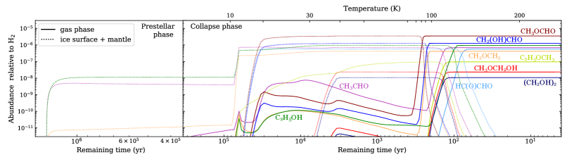
Figure 8: Evolution of the abundances of three-carbon species during the prestellar and the collapse phase of the simulation run A1. The time axis is reversed to better visualise the abundance evolution. Each color corresponds to a single species, with its abundance in the gas phase and on grain surfaces shown in solid and dotted lines, respectively.

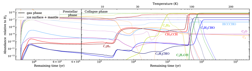
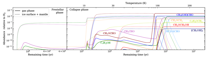
Figure 9: Evolution of the abundances of three-carbon species during the prestellar and the collapse phase of the simulation run A2. The time axis is reversed to better visualise the abundance evolution. Each color corresponds to a single species, with its abundance in the gas phase and on grain surfaces shown in solid and dotted lines, respectively.

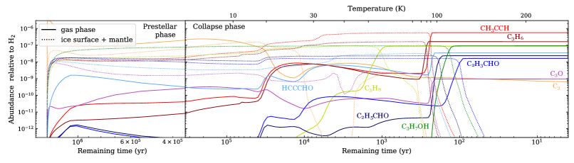
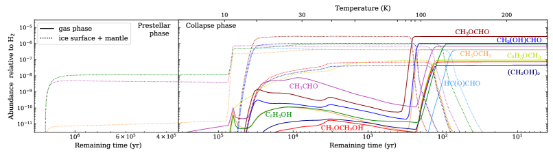
Figure 10: Evolution of the abundances of three-carbon species during the prestellar and the collapse phase of the simulation run B1. The time axis is reversed to better visualise the abundance evolution. Each color corresponds to a single species, with its abundance in the gas phase and on grain surfaces shown in solid and dotted lines, respectively.

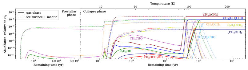
Figure 11: Evolution of the abundances of three-carbon species during the prestellar and the collapse phase of the simulation run B2. The time axis is reversed to better visualise the abundance evolution. Each color corresponds to a single species, with its abundance in the gas phase and on grain surfaces shown in solid and dotted lines, respectively.

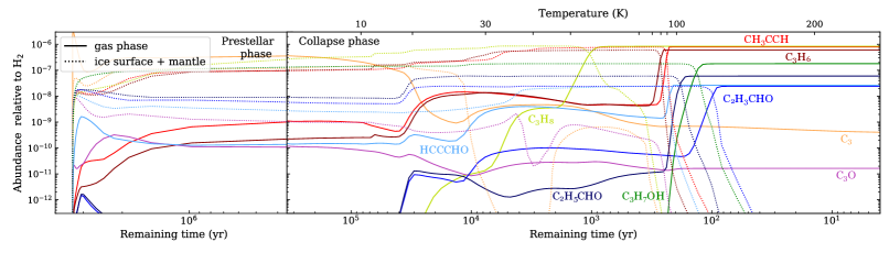
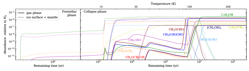
Figure 12: Evolution of the abundances of three-carbon species during the prestellar and the collapse phase of the simulation run C1. The time axis is reversed to better visualise the abundance evolution. Each color corresponds to a single species, with its abundance in the gas phase and on grain surfaces shown in solid and dotted lines, respectively.

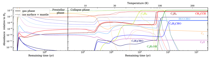
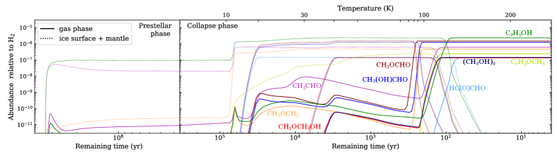
Figure 13: Evolution of the abundances of three-carbon species during the prestellar and the collapse phase of the simulation run C2. The time axis is reversed to better visualise the abundance evolution. Each color corresponds to a single species, with its abundance in the gas phase and on grain surfaces shown in solid and dotted lines, respectively.

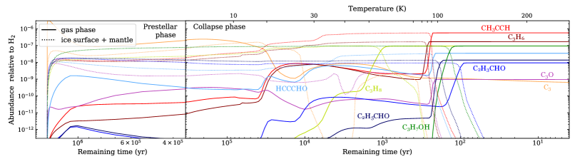
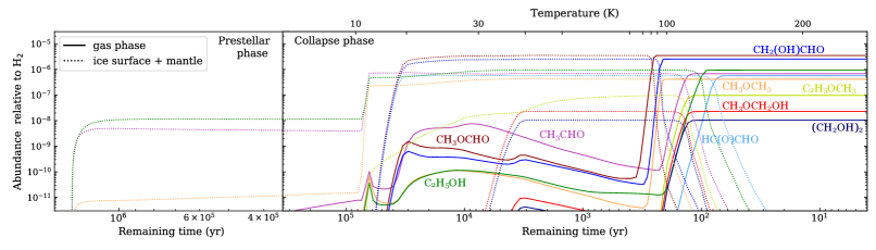
Figure 14: Evolution of the abundances of three-carbon species during the prestellar and the collapse phase of the simulation run D1. The time axis is reversed to better visualise the abundance evolution. Each color corresponds to a single species, with its abundance in the gas phase and on grain surfaces shown in solid and dotted lines, respectively.

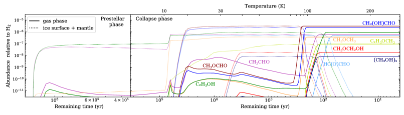
Figure 15: Evolution of the abundances of three-carbon species during the prestellar and the collapse phase of the simulation run D2. The time axis is reversed to better visualise the abundance evolution. Each color corresponds to a single species, with its abundance in the gas phase and on grain surfaces shown in solid and dotted lines, respectively.

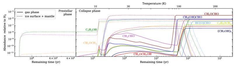
Figure 16: Evolution of the abundances of three-carbon species during the prestellar and the collapse phase of the simulation run E1. The time axis is reversed to better visualise the abundance evolution. Each color corresponds to a single species, with its abundance in the gas phase and on grain surfaces shown in solid and dotted lines, respectively.

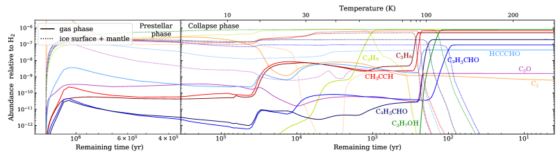
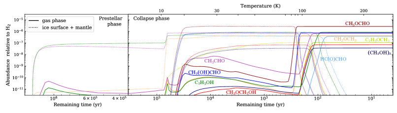
Figure 17: Evolution of the abundances of three-carbon species during the prestellar and the collapse phase of the simulation run E2. The time axis is reversed to better visualise the abundance evolution. Each color corresponds to a single species, with its abundance in the gas phase and on grain surfaces shown in solid and dotted lines, respectively.

Appendix E C₂H₃CHO line list

This section lists, in Table LABEL:app-linelist-C2H3CHO, the C₂H₃CHO transitions corresponding to the lines having an intensity above 3$\sigma$ in the observations. The firmly detected transitions, which are optically thin and unblended in the conditions of the best fit, are annotated with the letter ‘Y’.

Table 8: Line list of the observed C₂H₃CHO transitions above 3 $\sigma$.

Transition	Fitted	$\mathrm{\nu}$	$g_{\mathrm{u}}$	$E_{\mathrm{u}}$	$A_{\mathrm{ul}}$
$J(K_{\mathrm{a}},\ K_{\mathrm{c}})$ – $J^{\prime}(K_{\mathrm{a}}^{\prime},\ K_{\mathrm{c}}^{\prime})$		(GHz)		(K)	(s-1)
25( 1,24) – 24( 1,23)	Y	225.1917	51	143	$6.054\times 10^{-4}$
27( 0,27) – 26( 0,26)	Y	233.7577	55	159	$6.788\times 10^{-4}$
26( 1,25) – 25( 1,24)		233.9402	53	154	$6.793\times 10^{-4}$
26( 2,24) – 25( 2,23)	Y	235.9421	53	160	$6.947\times 10^{-4}$
27(10,17) – 26(10,16)		240.4387	55	367	$6.384\times 10^{-4}$
27(10,18) – 26(10,17)		240.4387	55	367	$6.384\times 10^{-4}$
27( 9,18) – 26( 9,17)		240.4537	55	328	$6.578\times 10^{-4}$
27( 9,19) – 26( 9,18)		240.4537	55	328	$6.578\times 10^{-4}$
27( 8,19) – 26( 8,18)	Y	240.4793	55	293	$6.752\times 10^{-4}$
27( 8,20) – 26( 8,19)	Y	240.4793	55	293	$6.752\times 10^{-4}$
27( 7,21) – 26( 7,20)	Y	240.5217	55	262	$6.908\times 10^{-4}$
27( 7,20) – 26( 7,19)	Y	240.5217	55	262	$6.908\times 10^{-4}$
27( 6,22) – 26( 6,21)		240.5929	55	236	$7.047\times 10^{-4}$
27( 6,21) – 26( 6,20)		240.5929	55	236	$7.047\times 10^{-4}$
28( 2,27) – 27( 2,26)		247.4024	57	181	$8.021\times 10^{-4}$
29( 0,29) – 28( 0,28)	Y	250.6283	59	182	$8.377\times 10^{-4}$
37( 3,35) – 36( 3,34)		329.5826	75	319	$1.902\times 10^{-3}$
37( 8,30) – 36( 8,29)		329.6375	75	432	$1.826\times 10^{-3}$
37( 8,29) – 36( 8,28)		329.6375	75	432	$1.826\times 10^{-3}$
37( 7,31) – 36( 7,30)	Y	329.7554	75	401	$1.850\times 10^{-3}$
37( 7,30) – 36( 7,29)	Y	329.7554	75	401	$1.850\times 10^{-3}$
37( 5,33) – 36( 5,32)		330.2566	75	352	$1.892\times 10^{-3}$
37( 5,32) – 36( 5,31)		330.3155	75	352	$1.893\times 10^{-3}$
37( 4,34) – 36( 4,33)	Y	330.5505	75	334	$1.909\times 10^{-3}$
37( 4,33) – 36( 4,32)		331.4060	75	334	$1.924\times 10^{-3}$
38( 2,37) – 37( 2,36)		333.8975	77	323	$1.985\times 10^{-3}$
37( 3,34) – 36( 3,33)	Y	334.7764	75	321	$1.994\times 10^{-3}$
39( 1,39) – 38( 1,38)		334.9111	79	325	$2.008\times 10^{-3}$
39( 0,39) – 38( 0,38)	Y	335.0926	79	325	$2.012\times 10^{-3}$
37( 2,35) – 36( 2,34)		335.4273	75	313	$2.012\times 10^{-3}$
38( 1,37) – 37( 1,36)	Y	336.4730	77	322	$2.032\times 10^{-3}$
38( 3,36) – 37( 3,35)		338.4007	77	336	$2.060\times 10^{-3}$
38( 7,32) – 37( 7,31)		338.6860	77	418	$2.008\times 10^{-3}$
38( 7,31) – 37( 7,30)		338.6860	77	418	$2.008\times 10^{-3}$
38( 4,35) – 37( 4,34)		339.5117	77	350	$2.071\times 10^{-3}$
38( 4,34) – 37( 4,33)		340.5275	77	351	$2.089\times 10^{-3}$
39( 2,38) – 38( 2,37)		342.4848	79	339	$2.143\times 10^{-3}$
40( 1,40) – 39( 1,39)		343.3917	81	342	$2.166\times 10^{-3}$
40( 0,40) – 39( 0,39)	Y	343.5483	81	342	$2.169\times 10^{-3}$
38( 3,35) – 37( 3,34)		344.0665	77	338	$2.166\times 10^{-3}$
38( 2,36) – 37( 2,35)		344.2952	77	330	$2.177\times 10^{-3}$
39( 1,38) – 38( 1,37)		344.8722	79	338	$2.190\times 10^{-3}$
39( 3,37) – 38( 3,36)		347.2066	79	352	$2.226\times 10^{-3}$
39( 8,32) – 38( 8,31)		347.4788	79	465	$2.151\times 10^{-3}$
39( 8,31) – 38( 8,30)		347.4788	79	465	$2.151\times 10^{-3}$
39( 7,33) – 38( 7,32)		347.6181	79	434	$2.176\times 10^{-3}$
39( 7,32) – 38( 7,31)		347.6181	79	434	$2.176\times 10^{-3}$
41( 1,41) – 40( 1,40)		351.8700	83	358	$2.331\times 10^{-3}$
41( 0,41) – 40( 0,40)		352.0051	83	358	$2.334\times 10^{-3}$
39( 2,37) – 38( 2,36)		353.1277	79	347	$2.350\times 10^{-3}$
40( 1,39) – 39( 1,38)		353.2630	81	355	$2.354\times 10^{-3}$
39( 3,36) – 38( 3,35)		353.3494	79	355	$2.348\times 10^{-3}$
40( 3,38) – 39( 3,37)	Y	355.9997	81	369	$2.401\times 10^{-3}$
40( 7,34) – 39( 7,33)		356.5518	81	451	$2.353\times 10^{-3}$
40( 7,33) – 39( 7,32)		356.5518	81	451	$2.353\times 10^{-3}$
40( 4,37) – 39( 4,36)	Y	357.4249	81	384	$2.420\times 10^{-3}$
41( 2,40) – 40( 2,39)	Y	359.6292	83	373	$2.483\times 10^{-3}$
42( 1,42) – 41( 1,41)		360.3463	85	376	$2.504\times 10^{-3}$
42( 0,42) – 41( 0,41)		360.4625	85	376	$2.506\times 10^{-3}$
40( 2,38) – 39( 2,37)		361.9237	81	364	$2.531\times 10^{-3}$
40( 3,37) – 39( 3,36)		362.6215	81	372	$2.539\times 10^{-3}$

Table 8: continued.

Appendix F C₃H₆ line list

This section lists, in Table LABEL:app-linelist-C3H6, the C₃H₆ transitions corresponding to the lines having an intensity above 3$\sigma$ in the observations. The firmly detected transitions, which are optically thin and unblended in the conditions of the best fit, are annotated with the letter ‘Y’.

Table 9: Line list of the observed C₃H₆ transitions above 3 $\sigma$.

Transition	Fitted	$\mathrm{\nu}$	$g_{\mathrm{u}}$	$E_{\mathrm{u}}$	$A_{\mathrm{ul}}$
$J(K_{\mathrm{a}},\ K_{\mathrm{c}})$ – $J^{\prime}(K_{\mathrm{a}}^{\prime},\ K_{\mathrm{c}}^{\prime})$		(GHz)		(K)	(s-1)
13( 2,12) – 12( 2,11) E		225.1013	108	83	$1.517\times 10^{-5}$
13( 2,12) – 12( 2,11) A		225.1024	108	83	$1.517\times 10^{-5}$
13( 1,12) – 12( 1,11) E		231.2205	108	80	$1.672\times 10^{-5}$
13( 1,12) – 12( 1,11) A		231.2233	108	80	$1.672\times 10^{-5}$
13( 2,11) – 12( 2,10) E		232.5859	108	85	$1.676\times 10^{-5}$
13( 2,11) – 12( 2,10) A		232.5869	108	85	$1.676\times 10^{-5}$
14( 0,14) – 13( 0,13) E	Y	235.2697	116	86	$1.772\times 10^{-5}$
14( 0,14) – 13( 0,13) A	Y	235.2714	116	86	$1.772\times 10^{-5}$
19( 1,18) – 18( 1,17) E	Y	331.5709	156	164	$4.986\times 10^{-5}$
19( 1,18) – 18( 1,17) A	Y	331.5751	156	164	$4.986\times 10^{-5}$
20( 1,20) – 19( 1,19) E		331.7410	164	170	$5.023\times 10^{-5}$
20( 1,20) – 19( 1,19) A		331.7421	164	170	$5.024\times 10^{-5}$
19( 8,11) – 18( 8,10) E		331.8207	156	274	$4.148\times 10^{-5}$
19( 8,12) – 18( 8,11) A		331.8207	156	274	$4.148\times 10^{-5}$
19( 8,11) – 18( 8,10) A		331.8207	156	274	$4.148\times 10^{-5}$
19( 7,13) – 18( 7,12) A		331.9592	156	248	$4.363\times 10^{-5}$
19( 7,12) – 18( 7,11) A		331.9592	156	248	$4.363\times 10^{-5}$
19( 3,17) – 18( 3,16) E	Y	332.1087	156	176	$4.926\times 10^{-5}$
19( 3,17) – 18( 3,16) A	Y	332.1091	156	176	$4.926\times 10^{-5}$
19( 6,14) – 18( 6,13) A		332.1877	156	224	$4.554\times 10^{-5}$
19( 6,13) – 18( 6,12) A		332.1890	156	224	$4.554\times 10^{-5}$
20( 0,20) – 19( 0,19) E		332.1893	164	170	$5.045\times 10^{-5}$
20( 0,20) – 19( 0,19) A		332.1909	164	170	$5.045\times 10^{-5}$
19( 6,14) – 18( 6,13) E		332.1909	156	224	$4.548\times 10^{-5}$
19( 6,13) – 18( 6,12) E		332.1909	156	224	$4.548\times 10^{-5}$
19( 5,15) – 18( 5,14) A		332.5731	156	204	$4.724\times 10^{-5}$
19( 5,15) – 18( 5,14) E		332.5773	156	204	$4.674\times 10^{-5}$
19( 5,14) – 18( 5,13) A		332.6150	156	204	$4.726\times 10^{-5}$
19( 5,14) – 18( 5,13) E		332.6154	156	204	$4.676\times 10^{-5}$
19( 4,16) – 18( 4,15) A		333.0380	156	188	$4.871\times 10^{-5}$
19( 4,16) – 18( 4,15) E		333.0396	156	188	$4.870\times 10^{-5}$
19( 4,15) – 18( 4,14) A		333.7945	156	188	$4.904\times 10^{-5}$
19( 4,15) – 18( 4,14) E		333.7959	156	188	$4.904\times 10^{-5}$
19( 3,16) – 18( 3,15) A		338.1148	156	177	$5.202\times 10^{-5}$
19( 3,16) – 18( 3,15) E		338.1152	156	177	$5.202\times 10^{-5}$
19( 2,17) – 18( 2,16) E	Y	340.8266	156	170	$5.403\times 10^{-5}$
19( 2,17) – 18( 2,16) A	Y	340.8293	156	170	$5.403\times 10^{-5}$
20( 2,19) – 19( 2,18) E		343.0971	164	181	$5.512\times 10^{-5}$
20( 2,19) – 19( 2,18) A		343.0990	164	181	$5.512\times 10^{-5}$
20( 1,19) – 19( 1,18) E	Y	347.7734	164	180	$5.760\times 10^{-5}$
20( 1,19) – 19( 1,18) A	Y	347.7777	164	180	$5.760\times 10^{-5}$
21( 1,21) – 20( 1,20) E		348.0323	172	187	$5.809\times 10^{-5}$
21( 1,21) – 20( 1,20) A		348.0335	172	187	$5.809\times 10^{-5}$
21( 0,21) – 20( 0,20) E	Y	348.3802	172	187	$5.827\times 10^{-5}$
21( 0,21) – 20( 0,20) A		348.3815	172	187	$5.827\times 10^{-5}$
20(10,11) – 19(10,10) E	Y	349.1524	164	356	$4.411\times 10^{-5}$
20(10,11) – 19(10,10) A	Y	349.1526	164	356	$4.412\times 10^{-5}$
20(10,10) – 19(10, 9) A	Y	349.1526	164	356	$4.412\times 10^{-5}$
20( 8,13) – 19( 8,12) A		349.3206	164	291	$4.948\times 10^{-5}$
20( 8,12) – 19( 8,11) A		349.3206	164	291	$4.948\times 10^{-5}$
20( 8,12) – 19( 8,11) E		349.3206	164	291	$4.948\times 10^{-5}$
20( 3,18) – 19( 3,17) E		349.4123	164	192	$5.757\times 10^{-5}$
20( 3,18) – 19( 3,17) A		349.4129	164	192	$5.757\times 10^{-5}$
20( 7,14) – 19( 7,13) A	Y	349.4842	164	264	$5.176\times 10^{-5}$
20( 7,13) – 19( 7,12) A	Y	349.4843	164	264	$5.176\times 10^{-5}$
20( 6,15) – 19( 6,14) A		349.7525	164	241	$5.379\times 10^{-5}$
20( 6,14) – 19( 6,13) A		349.7549	164	241	$5.379\times 10^{-5}$
20( 6,15) – 19( 6,14) E		349.7561	164	241	$5.358\times 10^{-5}$
20( 6,14) – 19( 6,13) E		349.7568	164	241	$5.358\times 10^{-5}$
20( 5,16) – 19( 5,15) A		350.1976	164	221	$5.563\times 10^{-5}$
20( 5,16) – 19( 5,15) E		350.2011	164	221	$5.542\times 10^{-5}$
20( 5,15) – 19( 5,14) A	Y	350.2639	164	221	$5.567\times 10^{-5}$
20( 5,15) – 19( 5,14) E	Y	350.2653	164	221	$5.545\times 10^{-5}$
20( 4,17) – 19( 4,16) A		350.6713	164	205	$5.720\times 10^{-5}$
20( 4,17) – 19( 4,16) E		350.6728	164	205	$5.720\times 10^{-5}$
20( 4,16) – 19( 4,15) A	Y	351.7358	164	205	$5.772\times 10^{-5}$
20( 4,16) – 19( 4,15) E	Y	351.7372	164	205	$5.772\times 10^{-5}$
20( 3,17) – 19( 3,16) A	Y	356.6568	164	194	$6.130\times 10^{-5}$
20( 3,17) – 19( 3,16) E	Y	356.6571	164	194	$6.130\times 10^{-5}$
20( 2,18) – 19( 2,17) E		358.4284	164	187	$6.296\times 10^{-5}$
20( 2,18) – 19( 2,17) A		358.4315	164	187	$6.298\times 10^{-5}$
21( 2,20) – 20( 2,19) E		359.7217	172	199	$6.365\times 10^{-5}$
21( 2,20) – 20( 2,19) A		359.7237	172	199	$6.365\times 10^{-5}$

Table 9: continued.