Robust and effective eSIF preconditioning for general SPD matrices

Abstract

We propose an unconditionally robust and highly effective preconditioner for general symmetric positive definite (SPD) matrices based on structured incomplete factorization (SIF), called enhanced SIF (eSIF) preconditioner. The original SIF strategy proposed recently derives a structured preconditioner by applying block diagonal preprocessing to the matrix and then compressing appropriate scaled off-diagonal blocks. Here, we use an enhanced scaling-and-compression strategy to design the new eSIF preconditioner. Some subtle modifications are made, such as the use of two-sided block triangular preprocessing. A practical multilevel eSIF scheme is then designed. We give rigorous analysis for both the enhanced scaling-and-compression strategy and the multilevel eSIF preconditioner. The new eSIF framework has some significant advantages and overcomes some major limitations of the SIF strategy. (i) With the same tolerance for compressing the off-diagonal blocks, the eSIF preconditioner can approximate the original matrix to a much higher accuracy. (ii) The new preconditioner leads to much more significant reductions of condition numbers due to an accelerated magnification effect for the decay in the singular values of the scaled off-diagonal blocks. (iii) With the new preconditioner, the eigenvalues of the preconditioned matrix are much better clustered around $1$. (iv) The multilevel eSIF preconditioner is further unconditionally robust or is guaranteed to be positive definite without the need of extra stabilization, while the multilevel SIF preconditioner has a strict requirement in order to preserve positive definiteness. Comprehensive numerical tests are used to show the advantages of the eSIF preconditioner in accelerating the convergence of iterative solutions.

Jianlin XiaRobust and effective eSIF preconditioning

15A23, 65F10, 65F30

1 Introduction

In this paper, we consider the design of an effective and robust preconditioning strategy for general dense symmetric positive definite (SPD) matrices. An effective preconditioner can significantly improve the convergence of iterative solutions. For an SPD matrix $A$, it is also desirable for the preconditioner to be robust or to preserve the positive definiteness. A commonly used strategy to design robust preconditioners is to apply modifications or incomplete/approximate Cholesky factorizations to $A$ together with some robustness or stability enhancement strategies (see, e.g., [2, 3, 4, 7, 10]).

In recent years, a powerful tool has been introduced into the design of robust SPD preconditioners and it is to use low-rank approximations for certain dense blocks in $A$, $A^{-1}$, or some factors of $A$. A common way is to directly approximate $A$ by so-called rank structured forms like the ones in [20, 23], but it is usually difficult to justify the performance of the resulting preconditioners. On the other hand, there are two types of methods that enable rigorous analysis of the effectiveness. One type is in [11, 12, 13, 18] based on low-rank strategies for approximating $A^{-1}$. Another type is in [1, 6, 8, 9, 14, 19, 21, 22] where approximate Cholesky factorizations are computed using low-rank approximations of relevant off-diagonal blocks. Both types of methods have been shown useful for many applications. A critical underlying reason (sometimes unnoticed in earlier work) behind the success of these preconditioners is actually to apply appropriate block diagonal scaling to $A$ first and then compress the resulting scaled off-diagonal blocks. A systematic way to formalize this is given in [21] as a so-called scaling-and-compression strategy and the resulting factorization is said to be a structured incomplete factorization (SIF). The preconditioning technique is called SIF preconditioning.

The basic idea of (one-level) SIF preconditioning is as follows [21]. Suppose $A$ is $N\times N$ and is partitioned as

(1) $$A\equiv\left(\begin{array}[c]{cc}A_{11}&A_{12}\\ A_{21}&A_{22}\end{array}\right).$$

where the diagonal blocks $A_{11}$ and $A_{22}$ have Cholesky factorizations of the forms

(2) $$A_{11}=L_{1}L_{1}^{T},\quad A_{22}=L_{2}L_{2}^{T}.$$

Then the inverses of these Cholesky factors are used to scale the off-diagonal blocks. That is, let

(3) $$C=L_{1}^{-1}A_{12}L_{2}^{-T}.$$

Suppose $C$ has singular values $\sigma_{1}\geq\sigma_{2}\geq\cdots\geq\sigma_{k}$ (which are actually all smaller than $1$), where $k$ is the smaller of the row and column sizes of $C$. Then the singular values $\sigma_{i}$ are truncated aggressively so as to enable the quick computation of a rank structured approximate factorization of $A$.

Thus, the SIF technique essentially employs block diagonal scaling to preprocess $A$ before relevant compression. This makes a significant difference as compared with standard rank-structured preconditioners that are based on direct off-diagonal compression. Accordingly, the SIF preconditioner has some attractive features, such as the convenient analysis of the performance, the convenient control of the approximation accuracy, and the nice effectiveness for preconditioning [21, 22]. In fact, if only $r$ largest singular values of $C$ are kept in its low-rank approximation, then the resulting preconditioner (called a one-level or prototype preconditioner) approximates $A$ with a relative accuracy bound $\sigma_{r+1}$. The preconditioner also produces a condition number $\frac{1+\sigma_{r+1}}{1-\sigma_{r+1}}$ for the preconditioned matrix. This idea can be repeatedly applied to the diagonal blocks to yield a practical multilevel SIF preconditioner.

A key idea for the effectiveness of the SIF preconditioner lies in a decay magnification effect [19, 21]. That is, although for a matrix $A$ where the singular values $\sigma_{i}$ of $C$ may only slightly decay, the condition number $\frac{1+\sigma_{r+1}}{1-\sigma_{r+1}}$ decays at a much faster rate to $1$. Thus, it is possible to use a relatively small truncation rank $r$ to get a structured preconditioner that is both effective and efficient to apply. A similar reason is also behind the effectiveness of those preconditioners in [11, 12, 13, 18, 19].

However, the SIF preconditioning has two major limitations. One is in the robustness. In the multilevel case, it needs a strict condition to avoid breakdown and ensure the existence or positive definiteness of the preconditioner. This condition needs either the condition number of $A$ to be reasonably small, the low-rank approximation tolerance to be small, or the number of levels to be small. These mean the sacrifice of either the applicability or the efficiency of the preconditioner, as pointed out in [22].

Another limitation is in the effectiveness. Although the condition number form $\frac{1+\sigma_{r+1}}{1-\sigma_{r+1}}$ has the decay magnification effect, if the decay of $\sigma_{i}$ is too slow, using small $r$ would not reduce the condition number too much. With small $r$, the eigenvalues of the preconditioned matrix may not closely cluster around $1$ either. The performance of the preconditioner can then be less satisfactory.

Therefore, the motivation of this work is to overcome both limitations of the SIF technique. We make enhancements in several aspects. First, we would like get rid of the condition in the SIF scheme that avoids breakdown. That is, we produce a type of structured preconditioners that is unconditionally robust or always positive definite. Second, we would like to approximate $A$ with better accuracies using the same truncation rank $r$. Next, we intend to accelerate the decay magnification effect in the condition number form. Lastly, we also try to improve the eigenvalue clustering of the preconditioned matrix.

Our idea to achieve these enhancements is to make some subtle changes to the original SIF scheme. Instead of block diagonal scaling, we use two-sided block triangular preprocessing which leads to an enhanced scaling-and-compression strategy. Then a low-rank approximation is still computed for $C$, but it is just used to accelerate computations related to Schur complements instead of off-diagonal blocks. (This will be made more precise in Section 2.) This strategy can be repeatedly applied to $A_{11}$ and $A_{22}$ in (1) so as to yield an efficient structured multilevel preconditioner.

This strategy makes it convenient to analyze the resulting preconditioners. The one-level preconditioner can now approximate $A\$with a relative accuracy bound $\sigma_{r+1}^{2}$ (in contrast with the bound $\sigma_{r+1}$ in the SIF case). The preconditioned matrix now has condition number $\frac{1}{1-\sigma_{r+1}^{2}}$, which is a significant improvement from $\frac{1+\sigma_{r+1}}{1-\sigma_{r+1}}$ due to the quadratic form $\sigma_{r+1}^{2}$ and the smaller numerator. Similar improvements are also achieved with the multilevel preconditioner.

Moreover, the eigenvalues of the preconditioned matrix are now more closely clustered around $1$. With the new one-level preconditioner, the eigenvalues are redistributed to $[1-\sigma_{r+1}^{2},1]$, with the eigenvalue $1$ of multiplicity $N-(k-r)$. In comparison, the one-level SIF preconditioner only brings the eigenvalues to the interval $[1-\sigma_{r+1},1+\sigma_{r+1}]$, with the eigenvalue $1$ of multiplicity $N-2(k-r)$. Similarly, the new multilevel preconditioner also greatly improves the eigenvalue clustering.

In addition, the multilevel generalization of the strategy always produces a positive definite preconditioner $\tilde{A}$ without the need of extra stabilization or diagonal compensation. In fact, the scheme has an automatic positive definiteness enhancement effect. That is, $\tilde{A}$ is equal to $A$ plus a positive semidefinite matrix. Thus, the new multilevel preconditioner is unconditionally robust.

Due to all these enhancements, the new preconditioner is called an enhanced SIF (eSIF) preconditioner. We give comprehensive analysis of the accuracy, robustness, and effectiveness of both the one-level and the multilevel eSIF preconditioners in Theorems 2.1, 2.3, 3.1 and 3.3. All the benefits combined yield significantly better effectiveness than the SIF scheme. With the same number of levels and the same truncation rank $r$, although the eSIF preconditioner is slightly more expensive to apply in each iteration step, the total iterative solution cost is much lower.

We also show some techniques to design a practical multilevel eSIF scheme and then analyze the efficiency and storage. The practical scheme avoids forming dense blocks like $C$ in (3) while enabling the convenient low-rank approximation of these blocks. It also produces structured factors defined by compact forms such as Householder vectors.

The performance of the preconditioner is illustrated in terms of some challenging test matrices including some from [21]. As compared with the SIF preconditioner, the eSIF preconditioner yields dramatic reductions in the number of conjugate gradient iterations.

The organization of the remaining sections is as follows. The enhanced scaling-and-compression strategy and the one-level eSIF preconditioner will be presented and analyzed in Section 2. The techniques and analysis will then be generalized to multiple levels in Section 3. Section 4 further gives the practical multilevel design of the preconditioning scheme and also analyzes the storage and costs. Comprehensive numerical tests will be given in Section 5, following by some conclusions and discussions in Section 6. For convenience, we list frequently used notation as follows.

• $\lambda(A)$ is used to represent an eigenvalue of $A$ (it is used in a general way and is not for any specific eigenvalue).

• $\kappa(A)$ denotes the 2-norm condition number of $A$.

• $\operatorname{diag}(\cdot)$ is used to mean a diagonal or block diagonal matrix constructed with the given diagonal entries or blocks.

• $I_{n}$ is the $n\times n$ identity matrix and is used to distinguish identity matrices of different sizes in some contexts.

2 Enhanced scaling-and-compression strategy and prototype eSIF preconditioner

We first give the enhanced scaling-and-compression strategy and analyze the resulting prototype eSIF preconditioner in terms of the accuracy, robustness, and effectiveness.

In the SIF preconditioner in [21], $A$ in (1) can be written as a factorized form as follows based on (2) and (3):

(4) $$A=\left(\begin{array}[c]{cc}L_{1}&\\ &L_{2}\end{array}\right)\left(\begin{array}[c]{cc}I&C\\ C^{T}&I\end{array}\right)\left(\begin{array}[c]{cc}L_{1}^{T}&\\ &L_{2}^{T}\end{array}\right),$$

where $\left(\begin{array}[c]{cc}I&C\\ C^{T}&I\end{array}\right)$ can be viewed as the result after the block diagonal preprocessing or scaling of $A$. $C$ is then approximated by a low-rank form so as to obtain a rank-structured approximate factorization of $A$.

Here, we make some subtle changes which will turn out to make a significant difference. Rewrite (4) in the following form:

(5) $$A=\left(\begin{array}[c]{cc}L_{1}&\\ L_{2}C^{T}&L_{2}\end{array}\right)\left(\begin{array}[c]{cc}I&\\ &I-C^{T}C\end{array}\right)\left(\begin{array}[c]{cc}L_{1}^{T}&CL_{2}^{T}\\ &L_{2}^{T}\end{array}\right).$$

Suppose $C$ is $m\times n$ and a rank-$r$ truncated SVD of $C$ is

(6) $$C\approx U_{1}\Sigma_{1}V_{1}^{T},$$

where $\Sigma_{1}=\operatorname{diag}(\sigma_{1},\sigma_{2},\ldots,\sigma_{r})$ is for the largest $r$ singular values $\sigma_{1}\geq\sigma_{2}\geq\cdots\geq\sigma_{r}$ of $C$. For later convenience, we also let the full SVD of $C$ be

(7) $$C=U\Sigma V^{T}=U_{1}\Sigma_{1}V_{1}^{T}+U_{2}\Sigma_{2}V_{2}^{T},$$

where $U=\left(\begin{array}[c]{cc}U_{1}&U_{2}\end{array}\right)$ and $V=\left(\begin{array}[c]{cc}V_{1}&V_{2}\end{array}\right)$ are orthogonal and $\Sigma_{2}$ is a (rectangular) diagonal matrix for the remaining singular values $\sigma_{r+1}\geq\cdots\geq\sigma_{\min\{m,n\}}$. We further suppose $\tau$ is a tolerance for truncating the singular values in (6). That is,

(8) $$\sigma_{r}\geq\tau\geq\sigma_{r+1}.$$

Note that all the singular values $\sigma_{i}$ of $C$ satisfy $\sigma_{i}<1$ [21], so $\tau<1$.

The apply (6) to $C^{T}C$ in (5) to get

$$C^{T}C\approx V_{1}\Sigma_{1}^{2}V_{1}^{T}.$$

In the meantime, we preserve the original form of $C$ in the two triangular factors in (5). Accordingly,

(9) $$A\approx\tilde{A}\equiv\left(\begin{array}[c]{cc}L_{1}&\\ L_{2}C^{T}&L_{2}\end{array}\right)\left(\begin{array}[c]{cc}I&\\ &I-V_{1}\Sigma_{1}^{2}V_{1}^{T}\end{array}\right)\left(\begin{array}[c]{cc}L_{1}^{T}&CL_{2}^{T}\\ &L_{2}^{T}\end{array}\right)$$

Suppose $\tilde{D}_{2}$ is the lower triangular Cholesky factor of $I-V_{1}\Sigma_{1}^{2}V_{1}^{T}$:

(10) $$I-V_{1}\Sigma_{1}^{2}V_{1}^{T}=\tilde{D}_{2}\tilde{D}_{2}^{T}.$$

Let

(11) $$\tilde{L}=\left(\begin{array}[c]{cc}L_{1}&\\ L_{2}C^{T}&L_{2}\end{array}\right)\left(\begin{array}[c]{cc}I&\\ &\tilde{D}_{2}\end{array}\right)=\left(\begin{array}[c]{cc}L_{1}&\\ &L_{2}\end{array}\right)\left(\begin{array}[c]{cc}I&\\ C^{T}&I\end{array}\right)\left(\begin{array}[c]{cc}I&\\ &\tilde{D}_{2}\end{array}\right).$$

Then we get a prototype (1-level) eSIF preconditioner

(12) $$\tilde{A}=\tilde{L}\tilde{L}^{T}.$$

This scheme can be understood as follows. Unlike in the SIF scheme where $A$ is preprocessed by the block diagonal factor $\left(\begin{array}[c]{cc}L_{1}&\\ &L_{2}\end{array}\right)$, here we use a block triangular factor $\left(\begin{array}[c]{cc}L_{1}&\\ L_{2}C^{T}&L_{2}\end{array}\right)$ to preprocess $A$. Note that it is still convenient to invert $\left(\begin{array}[c]{cc}L_{1}&\\ L_{2}C^{T}&L_{2}\end{array}\right)=\left(\begin{array}[c]{cc}L_{1}&\\ &L_{2}\end{array}\right)\left(\begin{array}[c]{cc}I&\\ C^{T}&I\end{array}\right)$ in linear system solution so the form of $C$ does not cause any substantial trouble. Also, we do not need to explicitly form or compress $C$. In addition, the Cholesky factor $\tilde{D}_{2}$ in (10) is only used for the purpose of analysis and does not need to be computed. The details will be given later in a more practical scheme in Section 4.

This leads to our enhanced scaling-and-compression strategy. We then analyze the properties of the resulting prototype eSIF preconditioner. Obviously, $\tilde{A}$ in (12) always exists and is positive definite. Furthermore, an additional benefit in the positive definiteness can be shown. We take a closer look at the positive definiteness of $\tilde{A}$ and also the accuracy of $\tilde{A}$ for approximating $A$.

Theorem 2.1.

Let $\tau$ be the truncation tolerance in (8). $\tilde{A}$ in (12) satisfies

$$\tilde{A}=A+E,$$

where $E$ is a positive semidefinite matrix and

(13) $$\frac{\|E\|_{2}}{\|A\|_{2}}\leq\sigma_{r+1}^{2}\leq\tau^{2}.$$

In addition,

(14) $$\frac{\|\tilde{L}-L\|_{2}}{\|L\|_{2}}\leq\frac{c\sqrt{1-\sigma_{n}^{2}}}{1-\sigma_{1}^{2}}\tau^{2},$$

where $L$ is the lower triangular Cholesky factor of $A$, $c=1+2\left\lceil\log_{2}n\right\rceil$, and $\sigma_{n}$ is either the $n$-th singular value of $C$ when $m\geq n$ or is $0$ otherwise. On the other hand, if $\tilde{D}_{2}$ in $\tilde{L}$ in (11) is replaced by $(I-V_{1}\Sigma_{1}^{2}V_{1}^{T})^{1/2}$ and $L$ is modified accordingly as $L=\left(\begin{array}[c]{cc}L_{1}&\\ L_{2}C^{T}&L_{2}(I-V\Sigma^{T}\Sigma V^{T})^{1/2}\end{array}\right)$ so that $A=LL^{T}$ still holds, then

(15) $$\frac{\|\tilde{L}-L\|_{2}}{\|L\|_{2}}<\tau^{2}.$$

Proof 2.2.

From (7) and (9), $\tilde{A}$ can be written as

$$\tilde{A} =\left(\begin{array}[c]{cc}A_{11}&A_{12}\\ A_{21}&L_{2}C^{T}CL_{2}^{T}+L_{2}(I-V_{1}\Sigma_{1}^{2}V_{1}^{T})L_{2}^{T}\end{array}\right)$$

$$=\left(\begin{array}[c]{cc}A_{11}&A_{12}\\ A_{21}&A_{22}+L_{2}(C^{T}C-V_{1}\Sigma_{1}^{2}V_{1}^{T})L_{2}^{T}\end{array}\right)$$

$$=\left(\begin{array}[c]{cc}A_{11}&A_{12}\\ A_{21}&A_{22}+L_{2}(V_{2}\Sigma_{2}^{T}\Sigma_{2}V_{2}^{T})L_{2}^{T}\end{array}\right)=A+E,$$

where $E=\operatorname*{diag}(0,L_{2}(V_{2}\Sigma_{2}^{T}\Sigma_{2}V_{2}^{T})L_{2}^{T})$ is positive semidefinite and

$$\|E\|_{2}=\|L_{2}(V_{2}\Sigma_{2}^{T}\Sigma_{2}V_{2}^{T})L_{2}^{T}\|_{2}\leq\sigma_{r+1}^{2}\|L_{2}\|_{2}^{2}=\sigma_{r+1}^{2}\|A_{22}\|_{2}\leq\sigma_{r+1}^{2}\|A\|_{2}.$$

Also, let $D_{2}D_{2}^{T}=I-V\Sigma^{T}\Sigma V^{T}$. Then $L=\left(\begin{array}[c]{cc}L_{1}&\\ L_{2}C^{T}&L_{2}D_{2}\end{array}\right)$. Thus,

(20) $$\|\tilde{L}-L\|_{2} =\left\|\left(\begin{array}[c]{cc}L_{1}&\\ L_{2}C^{T}&L_{2}\tilde{D}_{2}\end{array}\right)-\left(\begin{array}[c]{cc}L_{1}&\\ L_{2}C^{T}&L_{2}D_{2}\end{array}\right)\right\|_{2}$$

(23) $$=\left\|\left(\begin{array}[c]{cc}0&\\ &L_{2}(\tilde{D}_{2}-D_{2})\end{array}\right)\right\|_{2}\leq\|L\|_{2}\|\tilde{D}_{2}-D_{2}\|_{2}.$$

When $D_{2}$ is the lower triangular Cholesky factor of $I-V\Sigma^{T}\Sigma V^{T}$, an inequality in [21] gives

$$\|\tilde{D}_{2}-D_{2}\|_{2}\leq\frac{c\sqrt{1-\sigma_{n}^{2}}}{1-\sigma_{1}^{2}}\sigma_{r+1}^{2},\quad c=1+2\left\lceil\log_{2}n\right\rceil.$$

This leads to (14).

If $\tilde{D}_{2}$ in $\tilde{L}$ is replaced by $(I-V_{1}\Sigma_{1}^{2}V_{1}^{T})^{1/2}$ and $D_{2}$ is replaced by $(I-V\Sigma^{T}\Sigma V^{T})^{1/2}$, then

$$\|\tilde{D}_{2}-D_{2}\|_{2} =\|(I-V_{1}\Sigma_{1}^{2}V_{1}^{T})^{1/2}-(I-V\Sigma^{T}\Sigma V^{T})^{1/2}\|_{2}$$

$$=\|(I-\operatorname{diag}(\Sigma_{1}^{2},0))^{1/2}-(I-\Sigma^{T}\Sigma)^{1/2}\|_{2}$$

$$=1-\sqrt{1-\sigma_{r+1}^{2}}<\sigma_{r+1}^{2}.$$

Then following (20), we get (15).

This theorem gives both the accuracy and the robustness of the prototype eSIF preconditioner. Unlike the SIF framework where a similar prototype preconditioner has a relative accuracy bound $\tau$, here the bound is $\tau^{2}$ that is much more accurate. In addition, this theorem means the construction of $\tilde{A}$ automatically has a positive definiteness enhancement effect: it implicitly compensates $A$ by a positive semidefinite matrix $E$. This is similar to ideas in [9, 19]. Later, we will show that this effect further carries over to the multilevel generalization, which is not the case for the SIF preconditioner.

The effectiveness of the prototype eSIF preconditioner can be shown as follows.

Theorem 2.3.

The eigenvalues of $\tilde{L}^{-1}A\tilde{L}^{-T}$ are

$$\lambda(\tilde{L}^{-1}A\tilde{L}^{-T})=1-\sigma_{r+1}^{2},\ldots,1-\sigma_{k}^{2},\underset{N-(k-r)}{\underbrace{1,\ldots,1}},$$

where $k=\min\{m,n\}$. Accordingly,

$$\|\tilde{L}^{-1}A\tilde{L}^{-T}-I\|_{2} =\sigma_{r+1}^{2}\leq\tau^{2},$$

$$\kappa(\tilde{L}^{-1}A\tilde{L}^{-T}) =\frac{1}{1-\sigma_{r+1}^{2}}\leq\frac{1}{1-\tau^{2}}.$$

Proof 2.4.

It is not hard to verify

(24) $$\tilde{L}^{-1}A\tilde{L}^{-T}=\operatorname*{diag}(I_{N-n},\tilde{D}_{2}^{-1}(I_{n}-V\Sigma^{T}\Sigma V^{T})\tilde{D}_{2}^{-T}).$$

The eigenvalues of $\tilde{D}_{2}^{-1}(I_{n}-V\Sigma^{T}\Sigma V^{T})\tilde{D}_{2}^{-T}$ are

$$\lambda(\tilde{D}_{2}^{-1}(I_{n}-V\Sigma^{T}\Sigma V^{T})\tilde{D}_{2}^{-T}) =\lambda(\tilde{D}_{2}^{-T}\tilde{D}_{2}^{-1}(I_{n}-V\Sigma^{T}\Sigma V^{T}))$$

$$=\lambda((I_{n}-V_{1}\Sigma_{1}^{2}V_{1}^{T})^{-1}(I_{n}-V\Sigma^{T}\Sigma V^{T})).$$

Further derivations can be done via the Sherman-Morrison-Woodbury formula or in the following way:

$$(I_{n}-V_{1}\Sigma_{1}^{2}V_{1}^{T})^{-1}(I_{n}-V\Sigma^{T}\Sigma V^{T})$$

$$=\ (V(I_{n}-\operatorname{diag}(\Sigma_{1}^{2},0))V^{T})^{-1}V(I_{n}-\Sigma^{T}\Sigma)V^{T}$$

$$=\ V\operatorname{diag}((I_{r}-\Sigma_{1}^{2})^{-1},I_{n-r})(I_{n}-\Sigma^{T}\Sigma)V^{T}$$

$$=\ V\operatorname{diag}(I_{r},I_{n-r}-\Sigma_{2}^{T}\Sigma_{2})V^{T}.$$

Thus,

(25) $$\lambda(\tilde{D}_{2}^{-1}(I_{n}-V\Sigma^{T}\Sigma V^{T})\tilde{D}_{2}^{-T})=\lambda(\operatorname*{diag}(I_{r},I_{n-r}-\Sigma_{2}^{T}\Sigma_{2})),$$

which are just $1-\sigma_{r+1}^{2},\ldots,1-\sigma_{k}^{2},1$. The eigenvalue $1$ is a multiple eigenvalue. If $k=n$, then the eigenvalue $1$ in (25) has multiplicity $r$. If $k=m$, $I_{n-r}-\Sigma_{2}^{T}\Sigma_{2}$ also has $n-k$ eigenvalues equal to $1$ so the eigenvalue $1$ in (25) has multiplicity $n-(k-r)$. For both cases, the eigenvalue $1$ of $\tilde{L}^{-1}A\tilde{L}^{-T}$ has multiplicity $N-(k-r)$ according to (24).

To give an idea on the advantages of the prototype eSIF preconditioner over the corresponding prototype SIF preconditioner in [21], we compare the results in Table 1 with $\tilde{L}$ and $\tilde{A}$ from the eSIF or SIF scheme. The eSIF scheme yields a much higher approximation accuracy than SIF ($\tau^{2}$ vs. $\tau$) for both $\frac{\|A-\tilde{A}\|_{2}}{\|A\|_{2}}$ and $\|\tilde{L}^{-1}A\tilde{L}^{-T}-I\|_{2}$. The eigenvalues of the preconditioned matrix $\tilde{L}^{-1}A\tilde{L}^{-T}$ from eSIF are also much more closely clustered around $1$ and eSIF produces a lot more eigenvalues equal to $1$ than SIF. This is further illustrated in Figure 1.

Table 1: Comparison of prototype SIF and eSIF preconditioners that are used to produce $\tilde{L}$ and $\tilde{A}$, where $k=\min\{m,n\}$ and the results for the SIF preconditioner are from [21, 22].

	SIF	eSIF
$\frac{\|\tilde{A}-A\|_{2}}{\|A\|_{2}}$	$\leq\tau$	$\leq\tau^{2}$
$\frac{\|\tilde{L}-L\|_{2}}{\|L\|_{2}}$	$\leq\tau+\frac{c\sqrt{1-\sigma_{n}^{2}}}{1-\sigma_{1}^{2}}\tau^{2}$	$\leq\frac{c\sqrt{1-\sigma_{n}^{2}}}{1-\sigma_{1}^{2}}\tau^{2}$
$\lambda(\tilde{L}^{-1}A\tilde{L}^{-T})$	$1\pm\sigma_{r+1},\ldots,1\pm\sigma_{k},\underset{N-2(k-r)}{\underbrace{1,\ldots,1}}$	$1-\sigma_{r+1}^{2},\ldots,1-\sigma_{k}^{2},\underset{N-(k-r)}{\underbrace{1,\ldots,1}}$
$\|\tilde{L}^{-1}A\tilde{L}^{-T}-I\|_{2}$	$\sigma_{r+1}\leq\tau$	$\sigma_{r+1}^{2}\leq\tau^{2}$
$\kappa(\tilde{L}^{-1}A\tilde{L}^{-T})$	$\frac{1+\sigma_{r+1}}{1-\sigma_{r+1}}\leq\frac{1+\tau}{1-\tau}$	$\frac{1}{1-\sigma_{r+1}^{2}}\leq\frac{1}{1-\tau^{2}}$

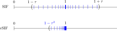
Figure 1: How the eigenvalues $\lambda(\tilde{L}^{-1}A\tilde{L}^{-T})$ cluster around $1$ when $\tilde{L}\tilde{L}^{T}$ is obtained with the prototype SIF and eSIF preconditioners.

Specifically, SIF produces $\kappa(\tilde{L}^{-1}A\tilde{L}^{-T})=\frac{1+\sigma_{r+1}}{1-\sigma_{r+1}}$, while eSIF leads to much smaller $\kappa(\tilde{L}^{-1}A\tilde{L}^{-T})=\frac{1}{1-\sigma_{r+1}^{2}}$. (Notice the quadratic term $\sigma_{r+1}^{2}$ in the denominator and the smaller numerator.) To further illustrate the difference in $\kappa(\tilde{L}^{-1}A\tilde{L}^{-T})$, we use an example like in [21]. In the example, the singular values of $C$ look like those in Figure 2(a) and are based on the analytical forms from a 5-point discrete Laplacian matrix [22]. The singular values of $C$ in (3) only slowly decay. Figure 2(b) shows $\kappa(\tilde{L}^{-1}A\tilde{L}^{-T})$ from both schemes. We can observe two things.

1. Like in SIF, the modest decay of the nonzero singular values $\sigma_{i}$ of $C$ is further dramatically magnified in $\frac{1}{1-\sigma_{i}^{2}}$. That is, even if $\sigma_{i}$ decays slowly, $\frac{1}{1-\sigma_{i}^{2}}$ decays much faster so that $\sigma_{i}$ can still be aggressively truncated so as to produce reasonably small $\kappa(\tilde{L}^{-1}A\tilde{L}^{-T})$. This is the decay magnifying effect like in [21].

2. Furthermore, the decay magnification effect from eSIF is more dramatic since$\ \frac{1}{1-\sigma_{i}^{2}}$ is smaller than $\frac{1+\sigma_{i}}{1-\sigma_{i}}$ by a factor of $(1+\sigma_{i})^{2}$. For a large range of $r$ values, eSIF gives much better condition numbers than SIF.

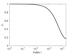
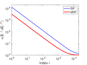
(a) Singular values $\sigma_{i}$ of $C$	(b) $\kappa(\tilde{L}^{-1}A\tilde{L}^{-T})$

Figure 2: For an example where the singular values $\sigma_{i}$ of $C$ slowly decay, how $\kappa(\tilde{L}^{-1}A\tilde{L}^{-T})$ decays when $\tilde{L}$ is from the prototype SIF or eSIF preconditioner obtained by truncating $\sigma_{i}$ with $r$ set to be $i$ in (b).

3 Multilevel eSIF preconditioner

The prototype preconditioner in the previous section still has two dense Cholesky factors $L_{1}$ and $L_{2}$ in (11). To get an efficient preconditioner, we generalize the prototype preconditioner to multiple levels. That is, apply it repeatedly to the diagonal blocks of $A$. For convenience, we use eSIF(1) to denote the prototype $1$-level eSIF scheme. A 2-level eSIF scheme or eSIF(2) uses eSIF(1) to obtain approximate factors $\tilde{L}_{1}\approx L_{1}$ and $\tilde{L}_{2}\approx L_{2}$ for (2). Similarly, an $l$-level eSIF scheme or eSIF($l$) uses eSIF($l-1$) to approximate $L_{1}$ and $L_{2}$. With a sufficient number of levels (usually $l=O(\log N)$), the finest level diagonal blocks are small enough and can be directly factorized. The overall resulting factor $\tilde{L}$ is an eSIF($l$) factor. The resulting approximation matrix $\tilde{A}$ is an eSIF($l$) preconditioner.

We prove that the eSIF($l$) preconditioner $\tilde{A}$ is always positive definite and show how accurate $\tilde{A}$ is for approximating $A$.

Theorem 3.1.

Let $\tau$ be the tolerance for any singular value truncation like (6)–(8) in the eSIF($l$) scheme. The approximate matrix $\tilde{A}$ resulting from eSIF($l$) is always positive definite and satisfies

(26) $$\tilde{A}=A+E,$$

where $E$ is a positive semidefinite matrix and

$$\frac{\|E\|_{2}}{\|A\|_{2}}\leq(1+\tau^{2})^{l}-1.$$

Proof 3.2.

We prove this by induction. $l=1$ corresponds to eSIF(1) and the result is in Theorem 2.1. Suppose the result holds for eSIF($l-1$) with $l>1$. Apply eSIF($l-1$) to $A_{11}$ and $A_{22}$ to get approximate Cholesky factors $\tilde{L}_{1}$ and $\tilde{L}_{2}$, respectively. By induction, we have

$$\tilde{L}_{1}\tilde{L}_{1}{}^{T}=A_{11}+E_{1},\quad\tilde{L}_{2}\tilde{L}_{2}{}^{T}=A_{22}+E_{2},$$

where $E_{1}$ and $E_{2}$ are positive semidefinite matrices satisfying

$$\|E_{1}\|_{2} \leq\left[(1+\tau^{2})^{l-1}-1\right]\|A_{11}\|_{2}\leq\left[(1+\tau^{2})^{l-1}-1\right]\|A\|_{2},$$

$$\|E_{2}\|_{2} \leq\left[(1+\tau^{2})^{l-1}-1\right]\|A_{22}\|_{2}\leq\left[(1+\tau^{2})^{l-1}-1\right]\|A\|_{2}.$$

Thus,

$$A\approx\left(\begin{array}[c]{cc}\tilde{L}_{1}\tilde{L}_{1}{}^{T}&A_{21}^{T}\\ A_{21}&\tilde{L}_{2}\tilde{L}_{2}{}^{T}\end{array}\right)=A+\operatorname*{diag}(E_{1},E_{2})\equiv\hat{A}.$$

Clearly, $\hat{A}$ is always positive definite.

Then apply eSIF(1) to $\hat{A}$ to yield

$$\hat{A}\approx\tilde{A}\equiv\tilde{L}\tilde{L}^{T},$$

where $\tilde{L}$ is the eSIF($l$) factor. With Theorem 2.1 applied to $\hat{A}$, we get

$$\tilde{A}=\hat{A}+\tilde{E},$$

where $\tilde{E}$ is a positive semidefinite matrix satisfying $\|\tilde{E}\|_{2}\leq\tau^{2}\|\hat{A}\|_{2}$. Then

$$\tilde{A}=A+(\operatorname*{diag}(E_{1},E_{2})+\tilde{E})\equiv A+E,$$

where $E=\operatorname*{diag}(E_{1},E_{2})+\tilde{E}$ is positive semidefinite. Thus, $\tilde{A}$ is positive definite and

$$\|E\|_{2} \leq\|\operatorname*{diag}(E_{1},E_{2})\|_{2}+\|\tilde{E}\|_{2}$$

$$\leq\|\operatorname*{diag}(E_{1},E_{2})\|_{2}+\tau^{2}\|\hat{A}\|_{2}$$

$$=\|\operatorname*{diag}(E_{1},E_{2})\|_{2}+\tau^{2}\|A+\operatorname*{diag}(E_{1},E_{2})\|_{2}$$

$$\leq\tau^{2}\|A\|_{2}+(1+\tau^{2})\|\operatorname*{diag}(E_{1},E_{2})\|_{2}$$

$$\leq\tau^{2}\|A\|_{2}+(1+\tau^{2})\left[(1+\tau^{2})^{l-1}-1\right]\|A\|_{2}$$

$$=\left[(1+\tau^{2})^{l}-1\right]\|A\|_{2}.$$

The result then holds by induction.

Thus, $\frac{\|E\|_{2}}{\|A\|_{2}}$ is roughly $O(l\tau^{2})$ for reasonable $\tau$, which indicates a very slow levelwise approximation error accumulation. Moreover, like eSIF($1$), eSIF($l$) also has a positive definiteness enhancement effect so that $\tilde{A}$ remains positive definite. In contract, the multilevel SIF scheme in [21] may breakdown due to the loss of positive definiteness.

Then we can look at the effectiveness of the eSIF($l$) preconditioner.

Theorem 3.3.

Let $\tau$ be the tolerance for any singular value truncation like (6)–(8) in the eSIF($l$) scheme and $\epsilon=\left[(1+\tau^{2})^{l}-1\right]\kappa(A)$. Let $\tilde{L}$ be the eSIF($l$) factor. Then the eigenvalues of the preconditioned matrix $\tilde{L}^{-1}A\tilde{L}^{-T}$ satisfy

(27) $$\frac{1}{1+\epsilon}\leq\lambda(\tilde{L}^{-1}A\tilde{L}^{-T})\leq 1.$$

Accordingly,

$$\|\tilde{L}^{-1}A\tilde{L}^{-T}-I\|_{2} \leq\frac{\epsilon}{1+\epsilon},$$

$$\kappa(\tilde{L}^{-1}A\tilde{L}^{-T}) \leq 1+\epsilon.$$

Proof 3.4.

Let $A=LL^{T}$ be the Cholesky factorization of $A$. With (26),

$$L^{-1}\tilde{A}L^{-T}=I+L^{-1}(\tilde{A}-A)L^{-T}=I+L^{-1}EL^{-T},$$

According to Theorem 3.1, $L^{-1}EL^{-T}$ is positive semidefinite. Thus, $\lambda(L^{-1}\tilde{A}L^{-T})\geq 1$.

Theorem 3.1 also yields

$$\|L^{-1}EL^{-T}\|_{2} \leq\|E\|_{2}\|L^{-1}\|_{2}\|L^{-T}\|_{2}$$

$$\leq\left[(1+\tau^{2})^{l}-1\right]\|A\|_{2}\|A^{-1}\|_{2}=\epsilon.$$

Therefore,

$$1\leq\lambda(L^{-1}\tilde{A}L^{-T})\leq 1+\epsilon.$$

Since the eigenvalues of $\tilde{L}^{-1}A\tilde{L}^{-T}$ are the inverses of those of $L^{-1}\tilde{A}L^{-T}$, we get (27).

A comparison of the multilevel eSIF and SIF preconditioners is given in Table 2. The multilevel eSIF preconditioner has several significant advantages over the SIF one.

1. The multilevel eSIF preconditioner is unconditionally robust or is guaranteed to be positive definite, while the SIF one needs a strict (or even impractical) condition to ensure the positive definiteness of the approximation. That is, the SIF one needs $\hat{\epsilon}\equiv\left[(1+\tau)^{l}-1\right]\kappa(A)<1$. This means $\tau$ needs to be small and/or the magnitudes of $l$ and $\kappa(A)$ cannot be very large.

2. The eSIF one gives a more accurate approximation to $A$ with a relative error bound $(1+\tau^{2})^{l}-1$ instead of $(1+\tau)^{l}-1$.

3. The eSIF one produces a much better condition number for the preconditioned matrix ($1+\epsilon$ vs. $\frac{1+\hat{\epsilon}}{1-\hat{\epsilon}}$ with $\epsilon$ further much smaller than $\hat{\epsilon}$).

4. The eSIF one further produces better eigenvalue clustering for the preconditioned matrix. The eigenvalues of the preconditioned matrix from eSIF lie in $[\frac{1}{1+\epsilon},1]$, while those from SIF lie in a much larger interval $[\frac{1}{1+\hat{\epsilon}},\frac{1}{1-\hat{\epsilon}}]$.

A combination of these advantages makes the eSIF preconditioner much more effective, as demonstrated later in numerical tests.

Table 2: Comparison of $l$-level SIF and eSIF preconditioners that are used to produce $\tilde{L}$ and $\tilde{A}$, where the results for the SIF preconditioner are from [21].

	SIF	eSIF
Existence/	Conditional	Unconditional
Positive definiteness	($\hat{\epsilon}\equiv\left[(1+\tau)^{l}-1\right]\kappa(A)<1$)
$\frac{\|\tilde{A}-A\|_{2}}{\|A\|_{2}}$	$\leq(1+\tau)^{l}-1$	$\leq(1+\tau^{2})^{l}-1$
$\lambda(\tilde{L}^{-1}A\tilde{L}^{-T})$	$\in[\frac{1}{1+\hat{\epsilon}},\frac{1}{1-\hat{\epsilon}}]$	$\in[\frac{1}{1+\epsilon},1]$
$\|\tilde{L}^{-1}A\tilde{L}^{-T}-I\|_{2}$	$\leq\frac{\hat{\epsilon}}{1-\hat{\epsilon}}$	$\leq\frac{\epsilon}{1+\epsilon}$
$\kappa(\tilde{L}^{-1}A\tilde{L}^{-T})$	$\leq\frac{1+\hat{\epsilon}}{1-\hat{\epsilon}}$	$\leq 1+\epsilon$

4 Practical eSIF($l$) scheme

In our discussions above, some steps are used for convenience and are not efficient for practical preconditioning. In the design of a practical scheme for eSIF($l$), we need to take care of the following points.

1. Avoid expensive dense Cholesky factorizations like in (10).

2. Avoid the explicit formation of $C$ in (3) (needed in (11)) which is too costly.

3. Compute the low-rank approximation of $C$ without the explicit form of $C$.

For the first point, we can let $Q$ be an orthogonal matrix extended from $V_{1}$ in (6) so that

$$Q^{T}V_{1}=\left(\begin{array}[c]{c}I\\ 0\end{array}\right).$$

Since $V_{1}$ has column size $r$ which is typically small for the purpose of preconditioning, $Q$ can be conveniently obtained with the aid of $r$ Householder vectors. Due to this, $Q$ is generally different from $V$ in (7). Then (10) can be replaced by

$$I-V_{1}\Sigma_{1}^{2}V_{1}^{T}=Q(I-\operatorname{diag}(\Sigma_{1}^{2},0))Q^{T}.$$

Accordingly, $\tilde{A}$ in (9) can be rewritten as

$$\tilde{A}=\left(\!\begin{array}[c]{cc}L_{1}&\\ L_{2}C^{T}&L_{2}\end{array}\!\right)\left(\!\begin{array}[c]{cc}I&\\ &Q\end{array}\!\right)\left(\!\begin{array}[c]{cc}I&\\ &I-\operatorname{diag}(\Sigma_{1}^{2},0)\end{array}\!\right)\left(\!\begin{array}[c]{cc}I&\\ &Q^{T}\end{array}\!\right)\left(\!\begin{array}[c]{cc}L_{1}^{T}&CL_{2}^{T}\\ &L_{2}^{T}\end{array}\!\right).$$

Thus, we can let

(34) $$\tilde{L} =\left(\!\begin{array}[c]{cc}L_{1}&\\ &L_{2}\end{array}\!\right)\left(\!\begin{array}[c]{cc}I&\\ C^{T}&I\end{array}\!\right)\left(\!\begin{array}[c]{cc}I&\\ &Q\tilde{\Sigma}_{1}\end{array}\!\right),\quad\text{with}$$

$$\tilde{\Sigma}_{1} =\operatorname*{diag}(\sqrt{1-\sigma_{1}^{2}},\ldots,\sqrt{1-\sigma_{r}^{2}},1,\ldots,1),$$

so that (12) still holds.

Next, we try to avoid the explicit formation of $C$ in (3) which is too expensive. Note (34) means

$$\tilde{L}^{-1}=\left(\!\begin{array}[c]{cc}I&\\ &\tilde{\Sigma}_{1}^{-1}Q^{T}\end{array}\!\right)\left(\!\begin{array}[c]{cc}I&\\ -C^{T}&I\end{array}\!\right)\left(\!\begin{array}[c]{cc}L_{1}^{-1}&\\ &L_{2}^{-1}\end{array}\!\right).$$

If $C$ is not formed but kept as the form in (3), then the application of $\tilde{L}^{-1}$ to a vector involves four smaller solution steps: one application of $L_{1}^{-1}$ to a vector, one application of $L_{1}^{-T}$ to a vector, and two applications of $L_{2}^{-1}$ to vectors. To reduce the number of such solutions, we rewrite $\tilde{L}$ in (34) as

(41) $$\tilde{L} =\left(\!\!\!\begin{array}[c]{cc}L_{1}&\\ &I\end{array}\!\!\!\right)\left(\!\!\!\begin{array}[c]{cc}I&\\ A_{12}^{T}L_{1}^{-T}&L_{2}\end{array}\!\!\!\right)\left(\!\!\!\begin{array}[c]{cc}I&\\ &Q\tilde{\Sigma}_{1}\end{array}\!\!\!\right)$$

(48) $$=\left(\!\!\!\begin{array}[c]{cc}L_{1}&\\ &I\end{array}\!\!\!\right)\left(\!\!\!\begin{array}[c]{cc}I&\\ A_{12}^{T}L_{1}^{-T}&I\end{array}\!\!\!\right)\left(\!\!\!\begin{array}[c]{cc}I&\\ &L_{2}Q\tilde{\Sigma}_{1}\end{array}\!\!\!\right).$$

$\tilde{L}^{-1}$ now has the following form and can be conveniently applied to a vector:

(49) $$\tilde{L}^{-1}=\left(\begin{array}[c]{cc}I&\\ &\tilde{\Sigma}_{1}^{-1}Q^{T}L_{2}^{-1}\end{array}\right)\left(\begin{array}[c]{cc}I&\\ -A_{12}^{T}L_{1}^{-T}&I\end{array}\right)\left(\begin{array}[c]{cc}L_{1}^{-1}&\\ &I\end{array}\right).$$

In fact, the application of $\tilde{L}^{-1}$ to a vector now just needs the applications of $L_{1}^{-1}$, $L_{1}^{-T}$, $L_{2}^{-1}$ to vectors. In the eSIF($l$) scheme, $L_{1}$ and $L_{2}$ are further approximated by structured factors from the eSIF($l-1$) scheme. In addition, $Q^{T}$ is a Householder matrix defined by $r$ Householder vectors and can be quickly applied to a vector. $A_{12}^{T}$ is just part of $A$. With (41), there is no need to form $C$ explicitly. From these discussions, it is also clear how $\tilde{L}^{-1}$ can be applied to vectors in actual preconditioning as structured solution.

Remark 4.1.

With the form of $\tilde{L}$ in (41), it is clear that (12) still holds for $\tilde{A}$ in (9). Thus, the approximation error result (13) in Theorem 2.1 and the effectiveness results in Theorem 2.3 remain the same. This further means that Theorems 3.1 and 3.3 for the multilevel scheme still hold.

Thirdly, although $C$ needs not to be formed, it still needs to be compressed so as to produce $\tilde{\Sigma}_{1}$ and $Q$ in (41). We use randomized SVD [15] that is based on matrix-vector products. That is, let

(50) $$Y=C^{T}Z=L_{2}^{-1}(A_{12}^{T}(L_{1}^{-1}Z)),$$

where $Z$ is an appropriate skinny random matrix with column size $r+\alpha$ and $\alpha$ is a small constant oversampling size. $Y$ can be used to extract $V_{1}$ approximately. After this, let

(51) $$T=CV_{1}=L_{1}^{-1}(A_{12}(L_{2}^{-T}V_{1})).$$

$TV_{1}^{T}$ essentially provides a low-rank approximation to $C$. Many studies of randomized SVDs in recent years have shown the reliability of this process. The tall and skinny matrix $T$ can then be used to quickly extract $r$ approximate leading singular values of $C$. Accordingly, this process provides an efficient way to get approximate $Q$ and $\tilde{\Sigma}_{1}$.

Computing $Y$ in (50) and $T$ in (51) uses linear solves in terms of $L_{1}$ and $L_{2}$ and matrix-vector multiplications in terms of $A_{12}$. When $\tilde{L}$ results from the eSIF($l$) scheme, $L_{1}$ and $L_{2}$ are approximated by structured eSIF($l-1$) factors.

We then study the costs to construct and apply the eSIF($l$) factor $\tilde{L}$ and the storage of $\tilde{L}$. In practical, we specify $r$ instead of $\tau$ in singular value truncations so as to explicitly control the cost. In the following estimates, the precise leading term is given for the application cost since it impacts the preconditioning cost.

Proposition 4.2.

Suppose $A$ is repeatedly bipartitioned into $l=\left\lfloor\log N\right\rfloor$ levels with the diagonal blocks at each partition level having the same size (for convenience). Let $\xi_{f}$ be the complexity to compute the eSIF($l$) factor $\tilde{L}$ where each intermediate compression step like (6) uses rank $r$. Let $\xi_{s}$ be the complexity to apply $\tilde{L}^{-1}$ to a vector. Then

$$\xi_{f}=O(rN^{2}),\quad\xi_{s}=2N^{2}+O(rN^{\log 3}).$$

The storage of $\tilde{L}$ is

$$\theta=O(rN\log N),$$

excluding any storage for the blocks of $A$.

Proof 4.3.

Let $\tilde{L}_{1}$ and $\tilde{L}_{2}$ be the eSIF($l-1$) factors that approximate $L_{1}$ and $L_{2}$, respectively. For the eSIF($l$) factor $\tilde{L}$, we use $\xi_{s}(N)$ to denote the cost to apply $\tilde{L}^{-1}$ to a vector. According to (49),

$$\xi_{s}(N)=3\xi_{s}(\frac{N}{2})+2(\frac{N}{2})^{2}+O(r\frac{N}{2}),$$

where the first term on the right-hand side is for applying $\tilde{L}_{1}^{-1}$, $\tilde{L}_{1}^{-T}$, $\tilde{L}_{2}^{-1}$ to vectors, the second term is the dominant cost for multiplying $A_{12}^{T}$ in (49) to a vector, and the third term is for the remaining costs (mainly to multiple $Q^{T}$ to a vector). This gives a recursive relationship which can be expanded to yield

$$\xi_{s}(N) =\frac{2}{3}N^{2}\sum_{i=1}^{l}\frac{3^{i}}{4^{i}}+O(rN\sum_{i=1}^{l}\frac{3^{i}}{2^{i}})$$

$$=2N^{2}+O(r3^{l})=2N^{2}+O(rN^{\log 3}).$$

Then consider the cost $\xi_{f}(N)$ to compute $\tilde{L}$. We have

$$\xi_{f}(N)=2\xi_{f}(\frac{N}{2})+4(r+\alpha)\xi_{s}(\frac{N}{2})+4(r+\alpha)(\frac{N}{2})^{2}+O(r^{2}\frac{N}{2}),$$

where the first term on the right-hand side is for constructing the eSIF($l-1$) factors $\tilde{L}_{1},\tilde{L}_{2}$, the second term is for applying the relevant inverses of these factors as in (50) and (51) during the randomized SVD (with $\alpha$ the small constant oversampling size), the third term is for multiplying $A_{12}^{T}$ and $A_{12}$ to vectors as in (50) and (51), and the last term is for the remaining costs. Based on this recursive relationship, we can similarly obtain $\xi_{f}(N)=O(rN^{2})$.

Finally, the storage $\theta(N)$ for $\tilde{L}$ (excluding the blocks of $A$) mainly includes the storage for $\tilde{L}_{1},\tilde{L}_{2}$ and the $r$ Householder vectors for $Q$ in (41):

$$\theta(N)=2\theta(\frac{N}{2})+O(rN).$$

At the finest level of the partitioning of $A$, it also needs the storage of $O(rN)$ for the Cholesky factors of the small diagonal blocks. Essentially, the actual storage at each level is then $O(rN)$ and the total storage is $\theta=O(rlN)$.

We can see that the storage for the structured factors is roughly linear in $N$ since $r$ is often fixed to be a small constant in preconditioning. The cost to construct the preconditioner is just a one-time cost. The cost of applying the preconditioner has a leading term $2N^{2}$. However, note that it costs about $2N^{2}$ to multiply $A$ with a vector in each iteration anyway. In the SIF case in [21], it also costs $O(rN^{2})$ to construct the multilevel preconditioner. The SIF application cost is lower but each iteration step still costs $O(N^{2})$ due to the matrix-vector multiplication. Furthermore, SIF preconditioners may not exist for some cases due to the loss of positive definiteness. In the next section, we can see that the multilevel eSIF preconditioner can often dramatically reduce the number of iterations so that it saves the total cost significantly.

5 Numerical experiments

We then show the performance of the multilevel eSIF preconditioner in accelerating the convergence of the preconditioned conjugate gradient method (PCG). We compare the following three preconditioners.

• bdiag: the block diagonal preconditioner.

• SIF: an SIF preconditioner from [21] (two versions of SIF preconditioners are given in [21], we use the one with better robustness).

• eSIF: the multilevel eSIF preconditioner.

In [21], it has been shown that SIF is generally much more effective than a preconditioner based on direct rank-structured approximations. Here, we would like to show how eSIF further outperforms SIF. The following notation is used to simplify the presentation of the test results.

• $\gamma=\frac{\|Ax-b\|_{2}}{\|b\|_{2}}$: 2-norm relative residual for a numerical solution $x$, with $b$ generated using the exact solution vector of all ones.

• $n_{\mathrm{iter}}$: total number of iterations to reach a certain accuracy for the relative residual.

• $A_{\mathrm{prec}}$: matrix preconditioned by the factors from the preconditioners (for example, $A_{\mathrm{prec}}=\tilde{L}^{-1}A\tilde{L}^{-T}$ in the eSIF case).

• $r$: numerical rank used in any low-rank approximation step in constructing SIF and eSIF.

• $l$: total number of levels in SIF and eSIF.

When SIF and eSIF are constructed, we use the same parameters $r$, $l$, and finest level diagonal block size. The preconditioner bdiag is constructed with the same diagonal block sizes as those of the finest level diagonal block sizes of SIF and eSIF.

Example 5.1.

We first test the methods on the matrix $A$ with the $(i,j)$ entry

$$A_{ij}=\frac{(ij)^{1/4}\pi}{20+0.8(i-j)^{2}},$$

which is modified from a test example in [21] to make it more challenging.

In the construction of SIF and eSIF, we use $r=5$. With the matrix size $N$ increases, $l$ increases accordingly for SIF and eSIF so that the finest level diagonal block size is fixed. Table 3 shows the results of PCG iterations to reach the tolerance $10^{-12}$ for the relative residual $\gamma$. Both SIF and eSIF help significantly reduce the condition numbers. The both make PCG converge much faster than using bdiag. eSIF is further much more effective than SIF and leads to $\kappa(A_{\mathrm{prec}})$ close to $1$. PCG with eSIF only needs few steps to reach the desired accuracy. The numbers of iterations are lower than with SIF by about 12 to 15 times.

Table 3: Example 5.1. Convergence results of PCG with bdiag, SIF, and eSIF preconditioners. (For the two largest matrices, it is very slow to form $A_{\mathrm{prec}}$, so the condition numbers are not computed.)

$N$		$1280$	$2560$	$5120$	$10,240$	$20,480$	$40,960$
$l$		$8$	$9$	$10$	$11$	$12$	$13$
$\kappa(A)$		$2.66e7$	$3.85e7$	$5.55e7$	$7.95e7$
$\kappa(A_{\rm prec})$	bdiag	$1.41e5$	$1.42e5$	$1.42e5$	$1.42e5$
	SIF	$5.03e1$	$5.03e1$	$5.03e1$	$5.03e1$
	eSIF	$1.01$	$1.01$	$1.02$	$1.02$
$n_{\mathrm{iter}}$	bdiag	$570$	$562$	$546$	$551$	$526$	$525$
	SIF	$57$	$60$	$61$	$60$	$60$	$60$
	eSIF	$4$	$4$	$4$	$4$	$4$	$5$
$\gamma$	bdiag	$9.65e\!-\!13$	$9.49e\!-\!13$	$9.50e\!-\!13$	$6.33e\!-\!13$	$7.89e\!-\!13$	$7.93e\!-\!13$
	SIF	$8.02e\!-\!13$	$8.42e\!-\!13$	$3.54e\!-\!13$	$9.36e\!-\!13$	$7.36e\!-\!13$	$8.28e\!-\!13$
	eSIF	$5.90e\!-\!15$	$5.48e\!-\!15$	$1.34e\!-\!13$	$4.28e\!-\!13$	$5.00e\!-\!14$	$9.61e\!-\!15$

Figure 3(a) shows the actual convergence behaviors for one matrix and Figure 3(b) reflects how the preconditioners change the eigenvalue distributions. With eSIF, the eigenvalues of $A_{\mathrm{prec}}$ are all closely clustered around $1$.

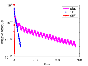
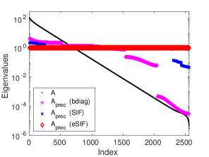
(a) Convergence	(b) Eigenvalues

Figure 3: Example 5.1. Convergence of PCG with bdiag, SIF, and eSIF preconditioners and eigenvalues of the preconditioned matrices for $N=2560$ in Table 3.

To confirm the efficiency of eSIF, we plot the storage requirement of eSIF and the cost to apply the preconditioner in each step. Since $r$ is fixed, the storage of eSIF is $O(N\log N)$, which is confirmed in Figure 4.

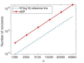
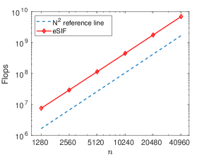
(a) Storage	(b) Application cost

Figure 4: Example 5.1. Storage for the structured factors of the eSIF preconditioner (excluding the storage for $A$) and the application cost.

Example 5.2.

In the second example, we consider to precondition some RBF (radial basis function) interpolation matrices which are known to be notoriously challenging for iterative methods due to the ill condition with some shape parameters (see, e.g., [5]). We consider the following four types of RBFs:

$$e^{-\varepsilon^{2}t^{2}},\quad\operatorname*{sech}\varepsilon t,\quad\frac{1}{\sqrt{1+\varepsilon^{2}t^{2}}},\quad\frac{1}{1+\varepsilon^{2}t^{2}},$$

where $\varepsilon$ is the shape parameter. The interpolation matrices are obtained with grid points $0,1,\ldots,N-1$.

We test the RBF interpolation matrices $A$ with various different shape parameters. With $N=1280$, $r=6$, and $l=8$, the performance of PCG to reach the tolerance $10^{-12}$ for $\gamma$ is given in Table 4. When the shape parameter $\varepsilon$ reduces, the condition numbers of the interpolation matrices increase quickly. SIF improves the condition numbers more significantly than bdiag. However, for smaller $\varepsilon$, the condition numbers resulting from both bdiag and SIF get much worse and the convergence of PCG slows down.

Table 4: Example 5.2. Convergence results of PCG using bdiag, SIF, and eSIF preconditioners with $r=6$ in SIF and eSIF.

RBF		$e^{-\varepsilon^{2}t^{2}}$			$\operatorname*{sech}\varepsilon t$
$\varepsilon$		$0.4$	$0.36$	$0.32$	$0.3$	$0.25$	$0.2$
$\kappa(A)$		$2.49e6$	$9.27e7$	$1.46e10$	$3.48e6$	$9.34e7$	$1.30e10$
$\kappa(A_{\rm prec})$	bdiag	$1.26e5$	$4.50e6$	$7.11e8$	$1.52e5$	$4.24e6$	$6.28e8$
	SIF	$2.38$	$2.11e3$	$2.14e6$	$1.34$	$5.02e2$	$7.58e5$
	eSIF	$1.00$	$1.00$	$1.00$	$1.00$	$1.00$	$1.30$
$n_{\mathrm{iter}}$	bdiag	$700$	$2193$	$4482$	$547$	$1271$	$3211$
	SIF	$15$	$107$	$549$	$9$	$52$	$282$
	eSIF	$1$	$1$	$2$	$1$	$1$	$3$
$\gamma$	bdiag	$8.82e\!-\!13$	$8.62e\!-\!13$	$8.97e\!-\!13$	$7.97e\!-\!13$	$9.28e\!-\!13$	$8.25e\!-\!13$
	SIF	$4.94e\!-\!13$	$5.16e\!-\!13$	$9.86e\!-\!13$	$4.02e\!-\!13$	$9.44e\!-\!13$	$9.91e\!-\!13$
	eSIF	$6.16e\!-\!16$	$7.34e\!-\!15$	$2.63e\!-\!16$	$6.96e\!-\!15$	$1.85e\!-\!13$	$4.91e\!-\!14$
RBF		$\frac{1}{\sqrt{1+\varepsilon^{2}t^{2}}}$			$\frac{1}{1+\varepsilon^{2}t^{2}}$
$\varepsilon$		$0.3$	$0.25$	$0.2$	$1/4$	$1/5$	$1/6$
$\kappa(A)$		$2.64e5$	$2.27e6$	$5.62e7$	$1.42e5$	$3.29e6$	$7.59e7$
$\kappa(A_{\rm prec})$	bdiag	$1.15e4$	$9.64e4$	$2.40e6$	$6.18e3$	$1.41e5$	$3.34e6$
	SIF	$1.74$	$6.30$	$2.22e2$	$1.94$	$2.66e1$	$8.91e2$
	eSIF	$1.00$	$1.00$	$1.26$	$1.00$	$1.00$	$1.03$
$n_{\mathrm{iter}}$	bdiag	$195$	$375$	$937$	$190$	$541$	$1222$
	SIF	$13$	$27$	$86$	$14$	$43$	$104$
	eSIF	$3$	$3$	$6$	$2$	$3$	$5$
$\gamma$	bdiag	$9.21e\!-\!13$	$7.19e\!-\!13$	$8.92e\!-\!13$	$9.84e\!-\!13$	$9.16e\!-\!13$	$7.52e\!-\!13$
	SIF	$4.23e\!-\!13$	$5.14e\!-\!13$	$6.20e\!-\!13$	$2.72e\!-\!13$	$7.15e\!-\!13$	$1.95e\!-\!13$
	eSIF	$1.77e\!-\!15$	$1.62e\!-\!15$	$8.16e\!-\!15$	$2.36e\!-\!13$	$5.58e\!-\!13$	$2.05e\!-\!15$

On the other hand, eSIF performs significantly better for all the cases. Dramatic reductions in the numbers of iterations can be observed. In Table 4, the number of PCG iterations with eSIF is up to $274$ times lower than with SIF and up to $2241$ times lower than with bdiag. Overall, PCG with eSIF takes just few iterations to reach the desired accuracy.

Figure 5(a) shows the actual convergence behaviors for one case and Figure 5(b) illustrates how the preconditioners improve the eigenvalue distribution. Again, the eigenvalue clustering with eSIF is much better.

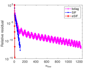
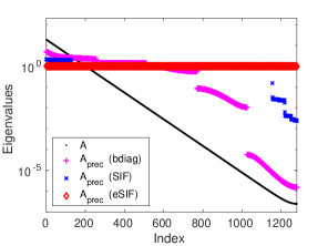
(a) Convergence	(b) Eigenvalues

Figure 5: Example 5.2. Convergence of PCG and eigenvalues of the preconditioned matrices for the case with RBF $\frac{1}{1+\varepsilon^{2}t^{2}}$, $\varepsilon=\frac{1}{6}$ in Table 4.

We also try different numerical ranks $r$ and the results are reported in Table 5. SIF is more sensitive to $r$. For some cases, SIF with $r=4$ leads to quite slow convergence of PCG. In contrast, eSIF remains very effective for the different $r$ choices and yields much faster convergence.

Table 5: Example 5.2. Convergence results of PCG using SIF and eSIF preconditioners with different $r$.

RBF			$e^{-\varepsilon^{2}t^{2}}$			$\operatorname*{sech}\varepsilon t$
$\varepsilon$			$0.3$	$0.25$	$0.2$	$1/4$	$1/5$	$1/6$
$\kappa(A_{\rm prec})$	$r=8$	SIF	$1.01$	$2.35$	$3.64e4$	$1.00$	$1.23$	$4.80e3$
		eSIF	$1.00$	$1.00$	$1.00$	$1.00$	$1.00$	$1.06$
	$r=4$	SIF	$5.17e2$	$7.51e4$	$6.94e7$	$1.41e2$	$4.61e4$	$1.82e7$
		eSIF	$1.00$	$1.00$	$5.58$	$1.00$	$1.01$	$1.58e2$
$n_{\mathrm{iter}}$	$r=8$	SIF	$5$	$13$	$245$	$4$	$7$	$69$
		eSIF	$1$	$1$	$1$	$1$	$1$	$2$
	$r=4$	SIF	$178$	$751$	$3972$	$92$	$410$	$1613$
		eSIF	$2$	$3$	$17$	$2$	$3$	$14$
$\gamma$	$r=8$	SIF	$7.95e\!-\!15$	$2.90e\!-\!13$	$4.95e\!-\!13$	$2.64e\!-\!15$	$3.18e\!-\!13$	$4.28e\!-\!13$
		eSIF	$6.89e\!-\!16$	$1.08e\!-\!15$	$1.23e\!-\!14$	$6.28e\!-\!15$	$1.85e\!-\!13$	$8.59e\!-\!13$
	$r=4$	SIF	$9.09e\!-\!13$	$9.42e\!-\!13$	$4.36e\!-\!11$	$8.11e\!-\!13$	$6.92e\!-\!13$	$6.06e\!-\!13$
		eSIF	$1.20e\!-\!15$	$4.63e\!-\!15$	$7.58e\!-\!13$	$9.14e\!-\!16$	$8.64e\!-\!14$	$6.33e\!-\!13$
RBF			$\frac{1}{\sqrt{1+\varepsilon^{2}t^{2}}}$			$\frac{1}{1+\varepsilon^{2}t^{2}}$
$\varepsilon$			$0.3$	$0.25$	$0.2$	$1/4$	$1/5$	$1/6$
$\kappa(A_{\rm prec})$	$r=8$	SIF	$1.39$	$3.66$	$1.06e2$	$1.45$	$6.32$	$6.21e1$
		eSIF	$1.00$	$1.00$	$1.00$	$1.00$	$1.00$	$1.00$
	$r=4$	SIF	$6.96e1$	$7.44e2$	$2.47e4$	$2.98$	$9.42e1$	$1.91e4$
		eSIF	$1.03$	$1.56$	$1.18$	$1.00$	$1.06$	$4.34$
$n_{\mathrm{iter}}$	$r=8$	SIF	$10$	$19$	$75$	$11$	$27$	$64$
		eSIF	$2$	$2$	$2$	$2$	$2$	$3$
	$r=4$	SIF	$77$	$224$	$761$	$19$	$87$	$368$
		eSIF	$5$	$8$	$19$	$4$	$5$	$14$
$\gamma$	$r=8$	SIF	$9.73e\!-\!14$	$7.71e\!-\!13$	$4.63e\!-\!13$	$1.11e\!-\!13$	$2.50e\!-\!13$	$6.97e\!-\!13$
		eSIF	$1.78e\!-\!15$	$2.19e\!-\!14$	$1.09e\!-\!13$	$1.44e\!-\!15$	$3.02e\!-\!15$	$1.95e\!-\!15$
	$r=4$	SIF	$5.93e\!-\!13$	$9.84e\!-\!13$	$9.21e\!-\!13$	$4.81e\!-\!13$	$9.20e\!-\!13$	$5.71e\!-\!13$
		eSIF	$8.38e\!-\!14$	$9.19e\!-\!13$	$1.87e\!-\!13$	$3.84e\!-\!15$	$2.67e\!-\!13$	$1.05e\!-\!13$

Example 5.3.

In the last example, we compare eSIF with SIF in terms of the following test matrices from different application backgrounds.

• MHD3200B ($N=3200$, $\kappa(A)=1.60e13$): The test matrix MHD3200B from the Matrix Market [16] treated as a dense matrix. $r=9$ and $l=8$ are used in the test.

• ElasSchur ($N=3198$, $\kappa(A)=8.91e6$): A Schur complement in the factorization of a discretized linear elasticity equation as used in [19]. The ratio of the so-called Lamé constants is $10^{5}$. The original sparse discretized matrix has size $5,113,602$ and $A$ corresponds to the last separator in the nested dissection ordering of the sparse matrix. $r=5$ and $l=9$ are used in the test.

• LinProg ($N=2301$, $\kappa(A)=2.09e11$): A test example in [21] from linear programming. The matrix is formed by $A=BDB^{T}$, where $B$ is from the linear programming test matrix set Meszaros in [17] and $D$ is a diagonal matrix with diagonal entries evenly located in $[10^{-5},1]$. $r=3$ and $l=9$ are used in the test.

• Gaussian ($N=4000$, $\kappa(A)=1.41e10$): a matrix of the form $sI+G$ with $G$ from the discretization of the Gaussian kernel $e^{-\frac{\|t_{i}-t_{j}\|_{2}}{2\mu^{2}}}$. Such matrices frequently appear in applications such as Gaussian processes. Here, $s=10^{-9}$, $\mu=2.5$ and the $t_{i}$ points are random points distributed in a long three dimensional rectangular parallelepiped. $r=20$ and $l=8$ are used in the test.

The convergence behaviors of PCG with SIF and eSIF preconditioners are given in Figure 6. Much faster convergence of PCG can be observed with eSIF. For the four matrices listed in the above order, the numbers of PCG iterations with SIF are about 11, 7, 7, and 21 times of those with eSIF, respectively.

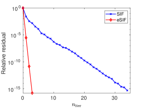
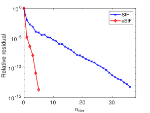
(a) MHD3200B	(b) ElasSchur
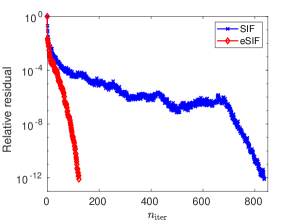
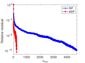
(c) LinProg	(d) Gaussian

Figure 6: Example 5.3. Convergence of PCG with SIF and eSIF preconditioners.

6 Conclusions

We have presented an eSIF framework that enhances a recent SIF preconditioner in multiple aspects. During the construction of the preconditioner, two-sided block triangular preprocessing is followed by low-rank approximations in appropriate computations. Analysis of both the prototype preconditioner and the practical multilevel extension is given. We are able to not only overcome a major bottleneck of potential loss of positive definiteness in the SIF scheme but also significantly improve the accuracy bounds, condition numbers, and eigenvalue distributions. Thorough comparisons in terms of the analysis and the test performance are given.

In our future work, we expect to explore new preprocessing and approximation strategies that can further improve the eigenvalue clustering and accelerate the decay magnification effect in the condition number. The current work successfully improves the relevant accuracy, condition number, and eigenvalue bounds by a significant amount (e.g., from $\frac{1+\hat{\epsilon}}{1-\hat{\epsilon}}$ to $1+\epsilon$ in Table 2 with $\epsilon$ much smaller than $\hat{\epsilon}$). We expect to further continue this trend and in the meantime keep the preconditioners convenient to apply. We will also explore the feasibility of extending our ideas to nonsymmetric and indefinite matrices.

References

- [1] E. Agullo, E. Darve, L. Giraud, and Y. Harness, Low-rank factorizations in data sparse hierarchical algorithms for preconditioning symmetric positive definite matrices, SIAM J. Matrix Anal. Appl. 39 (2018), pp. 1701–1725.
- [2] O. Axelsson and L. Kolotilina, Diagonally compensated reduction and related preconditioning methods, Numer. Linear Algebra Appl., 1 (1994), pp. 155–177.
- [3] M. Benzi, J. K. Cullum, and M. Tůma, Robust approximate inverse preconditioning for the conjugate gradient method, SIAM J. Sci. Comput., 22 (2000), pp. 1318–1332.
- [4] M. Benzi and M. Tůma, A robust incomplete factorization preconditioner for positive definite matrices, Numer. Linear Algebra Appl., 10 (2003), pp. 385–400.
- [5] J. P. Boyd and K. W. Gildersleeve, Numerical experiments on the condition number of the interpolation matrices for radial basis functions, Appl. Numer. Math., 61 (2011), pp. 443–459.
- [6] L. Cambier, C. Chen, E. G. Boman, S. Rajamanickam, R. S. Tuminaro, and E. Darve, An algebraic sparsified nested dissection algorithm using low-rank approximations, SIAM J. Matrix Anal. Appl., 41 (2020), pp. 715–746.
- [7] Z. Drmac, M. Omladic, and K. Veselic, On the perturbation of the Cholesky factorization, SIAM J. Matrix Anal. Appl., 15 (1994), pp. 1319–1332.
- [8] J. Feliu-Fabà, K. L. Ho, and L. Ying, Recursively preconditioned hierarchical interpolative factorization for elliptic partial differential equations, Commun. Math. Sci., 18 (2020), pp. 91–108.
- [9] M. Gu, X. S. Li, and P. Vassilevski, Direction-preserving and Schur-monotonic semiseparable approximations of symmetric positive definite matrices, SIAM J. Matrix Anal. Appl., 31 (2010), pp. 2650–2664.
- [10] D. S. Kershaw, The incomplete Cholesky–conjugate gradient method for the iterative solution of systems of linear equations, J. Comput. Phys., 26 (1978), pp. 43–65.
- [11] R. Li and Y. Saad, Divide and conquer low-rank preconditioners for symmetric matrices, SIAM J. Sci. Comput., 35 (2013); pp. A2069–A2095.
- [12] R. Li and Y. Saad, Low-rank correction methods for algebraic domain decomposition preconditioners, SIAM J. Matrix Anal. Appl., 38 (2017), pp. 807–828.
- [13] R. Li, Y. Xi, and Y. Saad, Schur complement based domain decomposition preconditioners with low-rank corrections, Numer. Linear Algebra Appl., 23 (2016), pp. 706–729.
- [14] S. Li, M. Gu, C. Wu, and J. Xia, New efficient and robust HSS Cholesky factorization of SPD matrices, SIAM J. Matrix Anal. Appl., 33 (2012), pp. 886–904.
- [15] E. Liberty, F. Woolfe, P. G. Martinsson, V. Rokhlin, and M. Tygert, Randomized algorithms for the low-rank approximation of matrices, Proc. Natl. Acad. Sci. USA, 104 (2007), pp. 20167–20172.
- [16] The Matrix Market, https://math.nist.gov/MatrixMarket.
- [17] The SuiteSparse Matrix Collection, http://faculty.cse.tamu.edu/davis/suitesparse.html.
- [18] Y. Xi, R. Li, and Y. Saad, An algebraic multilevel preconditioner with low-rank corrections for sparse symmetric matrices, SIAM J. Matrix Anal. Appl., 37 (2016), pp. 235–259.
- [19] J. Xia and M. Gu, Robust approximate Cholesky factorization of rank-structured symmetric positive definite matrices, SIAM J. Matrix Anal. Appl., 31 (2010), pp. 2899–2920.
- [20] J. Xia, S. Chandrasekaran, M. Gu, and X. S. Li, Fast algorithms for hierarchically semiseparable matrices, Numer. Linear Algebra Appl., 17 (2010), pp. 953–976.
- [21] J. Xia and Z. Xin, Effective and robust preconditioning of general SPD matrices via structured incomplete factorization, SIAM J. Matrix Anal. Appl., 38 (2017), pp. 1298–1322.
- [22] Z. Xin, J. Xia, S. Cauley, and V. Balakrishnan, Effectiveness and robustness revisited for a preconditioning technique based on structured incomplete factorization, Numer. Linear Algebra Appl., 27 (2020), e2294.
- [23] X. Xing and E. Chow, Preserving positive definiteness in hierarchically semiseparable matrix approximations, SIAM J. Matrix Anal. Appl., 39 (2018), pp. 829–855.