Lévy flights in steep potential wells: Langevin modeling versus direct response to energy landscapes

Abstract

We investigate the non-Langevin relative of the Lévy-driven Langevin random system, under an assumption that both systems share a common (asymptotic, stationary, steady-state) target pdf. The relaxation to equilibrium in the fractional Langevin-Fokker-Planck scenario results from an impact of confining conservative force fields on the random motion. A non-Langevin alternative has a built-in direct response of jump intensities to energy (potential) landscapes in which the process takes place. We revisit the problem of Lévy flights in superharmonic potential wells, with a focus on the extremally steep well regime, and address the issue of its (spectral) ”closeness” to the Lévy jump-type process confined in a finite enclosure with impenetrable (in particular reflecting) boundaries. The pertinent random system ”in a box/interval” might be expected to have a fractional Laplacian with suitable boundary conditions as a legitimate motion generator. It is not the case. Another problem is, that in contrast to Dirichlet boundary problems, a concept of reflecting boundary conditions and the path-wise implementation of the pertinent random process in the vicinity, or sharply at reflecting boundaries, are not unequivocally settled for Lévy processes. This ambiguity extends to nonlocal analogs of Neumann conditions for fractional generators, which do not comply with the traditional path-wise picture of reflection at the impenetrable boundary.

I Introduction

The Eliazar-Klafter targeted stochasticity concept, together with that of the reverse engineering (reconstruction of the stochastic process once a target pdf is a priori given), has been originally devised for Lévy-driven Langevin systems. Its generalization, discussed in gar ; gar1 , involves a non-Langevin alternative which associates with the Levy driver and the Langevin-induced target pdf, another (Feynman-Kac formula related) confinement mechanism for Lévy flights, based on a direct reponse to energy (potential) landscapes, instead of that to conservative forces.

We revisit the problem of Lévy motion in steep potential wells, analyzed in terms of a sequence of Fokker-Plack equations and their stationary solutions in Refs. dubkov ; dubkov1 and next path-wise in Ref. dybiec . Although we are ultimately interested in the extremal steepness regime, we need to mention that the above ”sequential” strategy has been introduced and next developed in a number of earlier publications chechkin ; chechkin1 ; chechkin2 , and summarized in a couple of review papers chechkin3 ; chechkin4 ; chechkin5 , see also chechkin6 .

An association of stationary probability density functions (pdfs), arising in the sequential superharmonic approximation (signatures of convergence), with steady-states of Lévy flights in a confined domain has been reported. The ”confined domain” notion has received an explicit interpretation of the infinitely deep potential well enclosure, denisov ; zoia , see also gar5 ; trap . This motivates our investigation of the semigroup (Feynman-Kac) motion scenario, which actually provides a non-Langevin alternative to the Langevin-Fokker-Planck relaxation process of dubkov ; dubkov1 ; dybiec . Our focus is on the possible asymptotic (growing steepness limit) emergence of a link with the problem of boundary data (Dirichlet versus Neumann, or absorbing versus reflecting) for the Lévy motion and its generator on the interval (or bounded/confined domain interpreted as the infinitely deep potential well), kulczycki .

One more important point should be raised. The infinite well enclosure for the random motion, and the limitation of the latter to the interval interior (impenetrability or inaccessibility of endpoints), are related to the notions of absorbing (Dirichlet) and reflecting (Neumann-type) boundaries. Interestingly, the discussion of dubkov ; dubkov1 ; dybiec definitely takes for granted the association of the ”confined domain” (like e.g. the infnitely deep potential well) boundaries with the reflection scenario for random motion, which is not a must, c.f. trap ; brownian ; gar4 , see also kulczycki . This point we shall briefly discuss in Section III of the present paper, where the ”confined domain” (and likewise the infinite well) will be associated with Dirichlet boundary conditions.

As well, for the above mentioned ”infinitely deep potential well problem”, no link has been established with the Neumann fractional Laplacian (whatever that is meant to be, neither with any convincing form of the Neumann condition), which is supposed to be a valid generator of the Lévy process in a bounded domain with reflecting boundaries.

This boundary issue can be consistently analyzed by employing the transformation of the fractional Fokker-Planck equation to the fractional Schrödinger-type equation (hence to the fractional semigroup). It is a properly tailored version of the technical tool, often used in the study case of the standard (Brownian) Fokker-Planck equation, but seldom addressed in the literature on confined Lévy processes. Since the superharmonic approximation seems to provide a suggestive method to understand what is possibly meant by the reflected Lévy process in the bounded domain (we restrict considerations to the interval on $R$), the pertinent transformation to the Schrödinger-type dynamics should in principle provide an approximation of this governed by the Neumann Laplacian and allow to identify features of the ”spectral closeness” of the pertinent operators (and fractional semigroups).

We shall investigate signatures of convergence for a sequence of confined Lévy processes on a line, in conservative force fields $\sim-x^{n-1}$ stemming from superharmonic potentials $U(x)\sim x^{n},x^{n}/n,nx^{n}$ with $n=2m\geq 2$. This is paralleled by a transformation of the related fractional Fokker-Planck operator $L^{*}=-|\Delta|^{\alpha/2}-\nabla[b(x)\cdot]$ into the fractional Schrödinger-type operator $\hat{H}=|\Delta|^{\alpha/2}+{\cal{V}}$, whose potential function is inferred from the knowledge of the square root of the stationary probability density $\rho_{*}(x)$ of the corresponding Markov process, according to ${\cal{V}}=-\rho_{*}^{-1/2}|\Delta|^{\alpha/2}\rho_{*}^{1/2}$. The pertinent $\rho_{*}^{1/2}(x)$ actually is the $L^{2}(R)$-normalized ground state function of $\hat{H}$.

The transformation of the Fokker-Planck operator (and likewise of the adjoint random motion generator) into the Schrödinger one is a celebrated tool in the study of Brownian relaxation processes. Recently, we have discussed at length various aspects of superharmonic approximations of the Brownian motion in the interval (and links of the latter problem with that of the ”infinitely deep potential well”). The Brownian route has been chosen as a playground for checking jeopardies and possible inadequacies of the (Schrödinger) transformation methodology brownian , prior to passing to an analysis of superharmonic approximations of Lévy flights ”in the infinitely deep well” (or interval), and technically more involved issue of reflected Lévy flights in the ”box” enclosure with impenetrable walls/barriers, along the lines indicated in Ref. smol .

Our discussion goes far beyond the technical (transformation proper) features. We deal here with physically different mechanisms for the response of the symmetric stable noise in one space dimension to external perturbations. To be considered as alternative response (and motion) scenarios: (i) set by conservative force potentials (motion in energy landscapes), or (ii) set directly by force fields. For both types of perturbations we shall preselect the Lévy driver and the stationary target pdf (common for both Langevin and non-Langevin motion scenarios), i.e. a probability density function $\rho_{*}(x)$ to which the random process asymptotically relaxes, once started with a suitable initial pdf $\rho_{0}(x)$: $\rho_{0}(x)\rightarrow\rho(x,t)\rightarrow\rho_{*}(x)$.

The Langevin approach stems from so-called targeted stochasticity concept, addressing the issue of an attainability of equilibria (generically not of the Boltzmann-type) for Lévy-driven Langevin systems, eliazar , see also gar ; gar1 ; gar2 . A related idea of reverse engineering, refers to a reconstruction (designing) of a Lévy-Langevin system, that would yield (relax to) a pre-defined target pdf. The pertinent random motion is known not to obey the detailed balance condition, balance ; balance1 , while the non-Langevin dynamics by construction does.

The non-Langevin approach, may be interpreted as an alternative version of the reverse engineering procedure (stochastic process reconstruction). It has roots in Ref. sokolov , see also gar ; gar1 ; gar2 , and involves the ”potential landscape” idea of Ref. kaleta . Given a stationary pdf $\rho_{*}(x)$ and the Lévy driver, one specifies the semigroup dynamics whose generator (fractional Laplacian plus a suitable potential function) has that pdf square root $\rho_{*}^{1/2}(x)$ as the positive-definite ground state function, vilela ; faris . The semigroup dynamics can be elevated to the fully-fledged stochastic process, governing the relaxation of a suitable $\rho(x,t)$ to the pre-defined $\rho_{*}(x)$, while maintaining the detailed balance condition.

I.1 Lévy driver.

Let us set the basic framework and the notation, to keep it uniform throughout the paper. A characteristic function of a random variable $X$ completely determines a probability distribution of that variable. If this distribution admits a density $\rho(x)$, we can write $<\exp(ipX)>=\int_{R}\rho(x)\exp(ipx)dx$ which, for infinitely divisible probability laws, gives rise to the famous Lévy-Khintchine formula. From now on, we concentrate on the integral part of the Lévy-Khintchine formula, which is responsible for arbitrary stochastic jump features:

$$F(p)=-\int_{-\infty}^{+\infty}\left[\exp(ipy)-1-\frac{ipy}{{1+y^{2}}}\right]\nu(dy),$$ (1)

where $\nu(dy)$ stands for the appropriate Lévy measure. The corresponding non-Gaussian Markov process is characterized by $<\exp(ipX_{t})>=\exp[-tF(p)]$ and, upon setting $\hat{p}=-i\nabla$ instead of $p$, yields an operator $F(\hat{p})$ which we interpret as the free Schrödindger-type Hamiltonian (for clarity of discussion, all dimensional constants generally are scaled away, note e.g. that in the Gaussian case $F(\hat{p})=-\Delta$).

We restrict further considerations to non-Gaussian random variables whose probability densities are centered and symmetric, e.g. a subclass of $\alpha$-stable distributions admitting a straightforward definition of the fractional noise generator

$$F(p)=|p|^{\alpha}\to F(\hat{p})\doteq|\Delta|^{\alpha/2}=(-\Delta)^{\alpha/2}.$$ (2)

We indicate that the adopted definition of the fractional Laplacian coincides with the negative of a suitable Riesz fractional derivative $\partial^{\alpha}/\partial|x|^{\alpha}\equiv\Delta^{\alpha/2}$, e.g. $(-\Delta)^{\alpha/2}=-\partial^{\alpha}/\partial|x|^{\alpha}$.

In the above, $0<\alpha<2$ stands for a stability index of the Lévy noise and the related stochastic process. The fractional Laplacian is a non-local pseudo-differential operator, by construction nonnegative and self-adjoint on a properly tailored domain. The induced jump-type dynamics is interpreted in terms of Lévy flights. In particular $\alpha=1$ refers to the Cauchy process, with the generator (for the record we list varied, commonly used notational conventions ) $F(\hat{p})=|\nabla|=|\Delta|^{1/2}=(-\Delta)^{1/2}\equiv\sqrt{-\Delta}$.

The pseudo-differential Fokker-Planck equation derives from the fractional semigroup $\exp(-t|\Delta|^{\alpha/2})$ and reads $\partial_{t}\rho=-|\Delta|^{\alpha/2}\rho$. That to be compared with the ”normal” Fokker-Planck equation for a freely diffusing particle (Wiener noise, with noise intensity $D=1$) $\partial_{t}\rho=\Delta\rho$, deriving from the semigroup $\exp(t\Delta)$.

An explicit integral form of the a pseudo-differential operator $|\Delta|^{\alpha/2}$, follows from (1) and (2):

$$(|\Delta|^{\alpha/2}f)(x)\,=\,-\int_{R}[f(x+y)-f(x)-{{y\,\nabla f(x)}\over{1+y^{2}}}]\,\nu_{\alpha}(dy).$$ (3)

This expression can greatly simplified, in view of the properties of the Lévy measure $\nu_{\mu}(dx)$. Namely, remembering that we overcome a singularity at $0$ by means of the Cauchy principal value of the integral, we may replace (3) by

$$|\Delta|^{\alpha/2}f(x)\,=(-\Delta)^{\alpha/2}f(x)=\,-\int_{R}[f(x+y)-f(x)]\nu_{\alpha}(dy)\,.$$ (4)

By changing an integration variable $y$ to $z=x+y$ and employing a direct connection with the Riesz fractional derivative of the order $\alpha$, we arrive at

$$|\Delta|^{\alpha/2}f(x)\,=\,-\mathcal{A}_{\alpha}\int_{R}{\frac{f(z)-f(x)}{|z-x|^{1+\alpha}}}\,dz.$$ (5)

where ${\cal{A}}_{\alpha}=\pi^{-1}\Gamma(\alpha+1)sin(\pi\alpha/2)$. The case of $\alpha=1$ refers to the Cauchy driver, with $\nu_{1}(y)=1/\pi y^{2}$.

We point out that, the evaluation of the singular integral in the definitions (4) and (5), needs some care. In Eq. (3) the problem is bypassed by means of the counter-term. An alternative definition:

$$|\Delta|^{\alpha/2}f(x)\,=(-\Delta)^{\alpha/2}f(x)={\frac{\mathcal{A}_{\alpha}}{2}}\int_{R}\frac{2f(x)-f(x+y)-f(x-y)}{|y|^{1+\alpha}}\,dy,$$ (6)

if employed in suitable function spaces, is by construction free of singularities and happens to be more amenable to computational procedures, kwasnicki ; kwa .

I.2 Langevin-induced fractional Fokker-Planck equation and motion generators.

In case of jump-type (Lévy) processes, a response of noise to conservative force fields may be quantified by mimicking the Brownian pattern. A popular reasoning, fogedby , employs a (formal) Langevin-type equation $\dot{x}=b(x)+B^{\alpha}(t)$ with a deterministic term $b(x)$ (a gradient function $b\sim-\nabla U$, presumed to encode Newtonian force fields) and the additive Lévy ”white noise” term. This leads to a fractional Fokker-Planck equation (fogedby , compare e.g. also olk ) governing the time evolution of the probability density function (pdf) $\rho(x,t)$ of the process:

$$\partial_{t}\rho=-\nabla(b\cdot\rho)-|\Delta|^{\alpha/2}\rho\,.$$ (7)

We emphasize a difference in sign in the second term, if compared with Eq. (4) of Ref. fogedby . There, the minus sign is absorbed in the adopted definition of the (Riesz) fractional derivative. Apart from the formal resemblance of operator symbols, we do not directly employ fractional derivatives in our discussion.

Let us assume that the fractional Fokker-Planck equation (7) admits a stationary solution $\rho_{*}(x)$, which is an asymptotic target $\rho(x,t)\rightarrow\rho_{*}(x)$ of the relaxation process. Then, a functional form of the time-independent drift $b(x)$ can be reconstructed by means of an indefinite integral

$$b(x)=-{\frac{\int dx\,|\Delta|^{\alpha/2}\rho_{*}(x)}{\rho_{*}(x)}}\,.$$ (8)

This is an ingredient of the reverse engineering procedure, eliazar ; gar ; gar1 , of reconstructing the random motion from the prescribed stationary (target) pdf, once the Lévy driver is pre-selected.

Anticipating further discussion, let us introduce some elements of the standard stochastic inventory. Let $p(y,s,x,t)=p(t-s,y,x),t>s\geq 0$ be the time-homogeneous transition density of the relaxation process (7), e.g.

$$\rho(x,t)=\int_{R}p(y,s,x,t)\rho(y,s)dy$$ (9)

We shall pass to the notation $p(t,y,x)$ to enable a direct comparison with the exemplary construction of the Ornstein-Uhlenbeck-Cauchy process in Ref. olk . Leaving aside unnecessary here mathematical details, we recall that the pertinent stochastic (jump-type) process is generated by the semigroup $T_{t}$, transforming continuous functions on $R$ (of the class $C_{0}(R)$) as follows:

$$T_{t}f(x)=\int_{R}p(t,x,y)f(y)=f(x,t)$$ (10)

In the mathematically oriented literature it is common to interpret $p(t,x,y)dy$ as a probability of getting from $x=X(0)$ to the (infinitesimal) vicinity of a point $y=X(t)$. Accordingly, $T_{t}f(x)=E_{x}[f(X_{t})]$ stands for a conditional expectation value of an ”observable” $f(x)$, evaluated over endpoints $X(t)=y$ of sample paths started from $x=X(0)$ and terminated at time $t$.

The semigroup $T_{t}=\exp(tL)$ has a generator

$$Lf(x)=\lim_{t\downarrow 0}{\frac{1}{t}}\left[\int p(t,x,y)f(y)dy-f(x)\right],$$ (11)

whose generic form reads

$$L=-|\Delta|^{\alpha/2}+b\nabla.$$ (12)

(We note its formal resemblance to the generator of the standard diffusion process (e.g. Brownian motion) $L_{B}=\Delta+b\nabla$.) Clearly, we have $\partial_{t}f(x,t)=L\,f(x,t)$.

The time evolution of probability measures and associated probability density functions $\rho(x,t)$ is governed by the adjoint semigroup $T^{*}_{t}=\exp(L^{*}t)$:

$$T_{t}^{*}\rho(x,t)=\int p(t,y,x)\rho(y)dy.$$ (13)

Accordingly, we have $\partial_{t}\rho(x,t)=L^{*}f(x,t)$, where

$$L^{*}=-|\Delta|^{\alpha/2}-\nabla(b\,\cdot)$$ (14)

comes from

$$L^{*}\rho(x)=\lim_{t\downarrow 0}{\frac{1}{t}}\left[\int p(t,y,x)\rho(y)dy-\rho(x)\right].$$ (15)

See e.g. Refs.fogedby ; olk for exemplary calculations.

We point out that transition pdfs in general are not symmetric functions of spatial variables: $p(t,x,y)\neq p(t,y,x)$. The order of variables clearly identifies the starting point (predecessor) and the terminal point (successor) for the stochastic process (bridge) connecting these points in the time interval of length $t$. In the mathematically oriented literature the pertinent symmetry is routinely restored, by passing from Lebesgue to weighted integration measures, see for example kaleta ; kaleta1 ; lorinczi .

II Non-Langevin approach.

II.1 Schrödinger’s interpolation problem.

We are inspired by apparent affinities between structural properties of probabilistic solutions of the so-called Schrödinger boundary data problem, zambrini ; gar3 , and the current research on conditioning of Markovian stochastic processes, of diffusion and jump-type, kaleta ; lorinczi ; gar4 ; gar5 ; gar6 , see also gar ; gar1 ; gar2 . The Schrödinger boundary data and interpolation problem is known to provide a unique Markovian interpolation between any two strictly positive probability densities, designed to form the input–output statistics data for a random process bound to run in a finite (observation) time interval.

The key input, if one attempts to reconstruct the pertinent Markovian dynamics, is to select the jointly continuous in space variables, positive and contractive semigroup kernel. Its choice is arbitrary, except for the strict positivity (not a must, but we keep this restriction in the present paper) and continuity demand. It is thus rather natural to ask for the most general stochastic interpolation, that is admitted under the above premises and the involved semigroups may refer not merely to diffusion scenarios of motion, but more generally to a broad family of non-Gaussian (specifically jump-type) processes.

The semigroup dynamics in question we infer from the classic notion of the Schrödinger semigroup $\exp(-t\hat{H})$, with a proviso that the semigroup generator $\hat{H}$ actually stands for a legitimate (up to scaled away physical constants) Hamiltonian operator, incorporating additive perturbations (by suitable potential functions) of either the traditional minus Laplacian, or the fractional Laplacian of the preceding subsections.

We are interested in Schrödinger-type operators of the form $\hat{H}_{\alpha}=(-\Delta)^{\alpha/2}+V(x)$, where $\hat{H}_{2}\equiv-\Delta+V(x)$, and the semigroups in question appear as members of the $\alpha$-family $\exp(-t\hat{H}_{\alpha})$, with $0<\alpha\leq 2$. Although, in our discussion the Schrödinger interpolation is restricted to a finite time interval $t\in[0,T]$, this restriction may be relaxed, once the solution (e.g. transition probability of the process) is in hands.

Roughly, the essence of the Schrödinger boundary data problem, zambrini , goes as follows. We consider Markovian propagation scenarios, with the input - output statistics data provided in terms of two strictly positive boundary densities $\rho(x,0)$ and $\rho(x,T)$, $T>0$, zambrini ; gar3 , that may be constrained to (integrated over) some Borel sets $A$ and $B$ contained in $R$. We interpret $\rho_{0}(A)$ and $\rho_{T}(B)$ as boundary data for a certain bivariate probability measure $m(A,B)$. Assume that the pertinent measure admits a transition probability density

$$m(x,y)=f(x)k(x,0,y,T)g(y)$$ (16)

with marginals $\int_{R}m(x,y)dy=\rho(x,0)$ and $\int_{R}m(x,y)dx=\rho(y,T)$ presumed to be associated with a certain dynamical process bound to run in a time interval $[0,T]$.

Here, $f(x)$ and $g(y)$ are the a priori unknown strictly positive functions, that need to be deduced from the imposed boundary data (i.e. marginals that are presumed to be known a priori). To this end, we should select any strictly positive, jointly continuous in space variables kernel function $k(x,0,y,T)$. We impose a restriction that $k(x,0,y,T)$ represents a certain strongly continuous dynamical semigroup kernel $k(y,s,x,t),\,0\leq s<t\leq T$, while specified at the time interval $[0,T]$ borders. This assumption will secure the Markov property of the sought for stochastic process. Actually, we shall consider time homogeneous processes generated by the semigroup $\exp[-(t-s)\hat{H}_{\alpha})$, with a kernel $k(t-s,y,x)$.

Under those circumstances, zambrini ; gar3 , once we define functions

$$\theta(x,t)=\{\exp[-(T-t)\hat{H}_{\alpha}]\,g\}(x)=\int k(x,t,y,T)g(y)dy$$ (17)

and

$$\theta_{*}(y,t)=\{\exp(-t\hat{H}_{\alpha})\,g\}(y)=\int k(x,0,y,t)f(x)dx$$ (18)

one can demonstrate the existence of a transition probability density (note that even if $k(t,y,x)=k(t,x,y)$ the symmetry property is not respected by $p(t,x,y)$ in below)

$$p(y,s,x,t)=k(y,s,x,t){\frac{\theta(x,t)}{\theta(y,s)}},$$ (19)

which implements a Markovian propagation of the probability density

$$\rho(x,t)=\theta(x,t)\theta_{*}(x,t),$$ (20)

according to the pattern

$$\rho(x,t)=\int p(y,s,x,t)\rho(y,s)dy=\theta(x,t)\int k(y,s,x,t)\theta_{*}(y,s)dy=\theta(x,t)\theta_{*}(x,t),$$ (21)

providing an interpolation between the prescribed boundary data in the time interval $[0,T]$.

Here we note the exploitation of the semigroup property, zambrini , in propagation formulas (17). Namely, for $0<s<t<T$, we have

$$\theta(x,s)=\int k(x,s,y,T)g(y)dy=\int\int k(x,s,z,t)k(z,t,y,T)g(y)dydz=\int k(x,s,z,t)\theta(z,t)dz$$ (22)

and

$$\theta_{*}(y,t)=\int k(x,0,y,t)f(x)dx=\int\int k(x,0,z,s)k(z,s,y,t)f(x)dxdz=\int k(z,s,y,t)\theta_{*}(z,s)dz$$ (23)

For a given semigroup $\exp(-t\hat{H}_{\alpha})$ which is characterized by its Hamiltonian generator $\hat{H}_{\alpha}$, the kernel $\exp(-t\hat{H}_{\alpha})(y,x)=k(t,y,x)$ and the emerging transition probability density $p(t,y,x)$ of the time homogeneous stochastic process are unique in view of the uniqueness of solutions $f(x)$ and $g(y)$ of the Schrödinger boundary data problem, zambrini . In the case of Markov processes, the knowledge of the transition probability density $p(y,s,x,t)$ (here $p(t-s,y,x)$) for all intermediate times $0\leq s<t\leq T$ suffices for the derivation of all other relevant characteristics of random motion.

Further exploiting the Schrödinger semigroup lore, and their Hamiltonian generators, we can write evolution equations for functions (17) in a form displaying an intimate link with Schrödinger-type equations. Namely, while in the interval $[0,T]$, gar6 , se e.g (17) and (18), we have $\partial_{t}\theta_{*}=-\hat{H}\theta_{*}$ and $\partial_{t}\theta=\hat{H}\theta$, where $\hat{H}=\hat{H}_{\alpha}=|\Delta|^{\alpha/2}+V$. Accordingly, gar3 :

$$\partial_{t}\theta_{*}=-|\Delta|^{\alpha/2}\theta_{*}-V\theta_{*}$$ (24)

and

$$\partial_{t}\theta=|\Delta|^{\alpha/2}\theta+V\theta.$$ (25)

For comparison, we indicate that the Brownian version of Eqs. (24) and (25) would have the form (up to scaled away physical constants) $\partial_{t}\theta_{*}=\Delta\theta_{*}-V\theta_{*}$ and $\partial_{t}\theta=-\Delta\theta+V\theta$ respectively.

Remark 1: At this point let us recall basic (Brownian) intuitions that underly the the implicit path integral formalism for Lévy flights. Namely, operators of the form (the diffusion coefficient $D$ is scaled away, typically a dimensionless form $D=1/2$ or $D=1$ is used to simplify calculations) $\hat{H}=-\Delta+V\geq 0$ with $V\geq 0$ give rise to transition kernels of diffusion -type Markovian processes with killing (absorption), whose rate is determined by the value of $V(x)$ at $x\in R$. This interpretation stems from the celebrated Feynman-Kac (path integration) formula, which assigns to $\exp(-\hat{H}t)$ the positive integral kernel

$$k(x,s,y,t)=[\exp(-(t-s)(-\Delta+V)](y,x)=\int\exp[-\int_{s}^{t}V(\omega(\tau))d\tau]\,d\mu_{s,y,x,t}(\omega)$$

In terms of Wiener paths the kernel is constructed as a path integral over paths which get killed at a point $X_{t}=x$, with an extinction probability $V(x)dt$ in the time interval$(t,t+dt)$. The killed path is henceforth removed from the ensemble of on-going Wiener paths. The exponential factor $\exp[-\int_{s}^{t}V(\omega(\tau))d\tau]$ is here responsible for a proper redistribution of Wiener paths, so that the evolution rule

$$f(x,t)=(\exp(-t\hat{H})]f)(x)=\int_{R^{n}}k(x,0;y,t)f(y)dy=E^{x}[f(X_{t})]=E^{x}[f(X_{t})\exp(-\int_{0}^{t}V(X_{s})ds)],$$

with $\hat{H}=-\Delta+V$, is well defined as an expectation value of the killed process $X(t)$, started at time zero, at $x\in R$.

Anticipating further discussion, we point out that the latter (Feynman-Kac) formula admits a generalization to Lévy processes, provided we pass to the transition kernel of the semigroup $\exp(-t\hat{H})$ with $\hat{H}=\hat{H}_{\alpha}=|\Delta|^{\alpha/2}+V$. Then, the path measure needs to be adopted to the jump-type setting, with sample paths of the Lévy process replacing the Wiener ones, see e.g. kaleta ; kaleta1 ; lorinczi ; lorinczi0 . The pertinent expectation is taken with respect to the path measure of the $\alpha$-stable process.

We note that in Ref. kaleta the function $V(x)$ is interpreted as delineating a potential landscape in which the random motion takes place.

II.2 Conditioned Lévy flights.

We have not yet specified any restrictions upon the properties of the potential function $V(x)$, nor its concrete functional form. In the present paper, the potential is expected to be a continuouus function and show up definite confining properties, which we adopt after kaleta , by demanding $\lim_{|x|\rightarrow\infty}V(x)=\infty$. Then, the Hamiltonian operator $\hat{H}_{\alpha}$ generically admits a positive ground state function $\varphi_{0}(x)$ with an isolated bottom eigenvalue $\lambda_{0}$ (typically a fully discrete spectrum is admitted).

With this proviso, let us invert our reasoning and consider evolution equations (24) and (25), with initial/terminal data $g(x)$ and $f(x)$ respectively. This specifies the Schrödinger interpolation of $\rho(x,t)=\theta(x,t)\theta_{*}(x,t)$ in the time interval $[0,T]$.

At this point, we shall narrow the generality of the addressed Schrödinger boundary data and interpolation problem, by assuming that actually for all $t\in[0,T]$ we have

$$\theta(x,t)=\exp(t\lambda_{0})\,\varphi_{0}(x)$$ (26)

where $\hat{H}_{\alpha}\varphi_{0}(x)=\lambda_{0}\varphi_{0}(x)$. Accordingly (we interchangeably use $|\Delta|^{\alpha/2}$ or $(-\Delta)^{\alpha/2}$):

$${\cal{V}}(x)=V(x)-\lambda_{0}=-{\frac{1}{\varphi_{0}(x)}}\,(-\Delta)^{\alpha/2}\varphi_{0}(x).$$ (27)

We point out a formal appearance of the potential function ${\cal{V}}(x)$ in the specific form, repeatedly invoked in our earlier papers, ${\cal{V}}(x)=-\rho_{*}^{-1/2}|\Delta|^{\alpha/2}\rho_{*}^{1/2}$, here specialized to the Cauchy case $\alpha=1$.

Let us indicate that the subtraction of $\lambda_{0}$ from the potential $V(x)$ is a standard way to assign the eigenvalue zero to the ground state function $\varphi_{0}(x)$ of the ”renormalized” Hamiltonian $\hat{H}-\lambda_{0}$, c.f. kaleta ; gar4 ; vilela ; faris . In reverse, it is the functional form of the right-hand-side of Eq. (27), which guarantees that $\hat{H}_{\alpha}^{ren}=\hat{H}_{\alpha}-\lambda_{0}=(-\Delta)^{\alpha/2}+{\cal{V}}(x)$ actually assigns the eigenvalue zero to the eigenfunction $\varphi_{0}(x)$.

Interestingly, a substitution of (26) to Eq. (19) implies

$$p(y,s,x,t)=\exp[\lambda_{0}(t-s)]\,k(y,s,x,t){\frac{\varphi_{0}(x)}{\varphi_{0}(y)}}.$$ (28)

This is a canonical functional form of the transition probability density for so-called ground state transformed jump-type process, whose probability density function $\rho(x,t)$ asymptotically relaxes to

$$\rho_{*}(x)={\frac{\varphi^{2}_{0}(x)}{\int\varphi^{2}_{0}(y)\,dy}}.$$ (29)

A detailed analysis of a number of exemplary cases can be found in Refs. gar3 ; gar4 ; gar5 ; gar6 ; vilela ; faris , where $\rho_{*}^{1/2}(x)$ notationally replaces $\varphi_{0}(x)/\sqrt{\int\varphi^{2}_{0}(y)dy}$. Accordingly, the compatibility condition (27) (the functional form of ${\cal{V}}(x)$ determines the functional form of $\rho_{*}^{1/2}(x)$ and in reverse) reads: ${\cal{V}}=-(|\Delta|^{\alpha/2}\rho_{*}^{1/2})/\rho_{*}^{1/2}$.

Remark 2: In the mathematical literature, kaleta ; kaleta1 ; lorinczi , the transition probability density (28) is usually transformed to the symmetric form (presuming $k(t,x,y)=k(t,y,x)$):

$$\tilde{p}(t,x,y)=\tilde{p}(t,y,x)=\frac{e^{\lambda_{0}t}k(t,x,y)}{\varphi_{0}(x)\varphi_{0}(y)}$$ (30)

with the proviso that the appropriate function space is not $L^{2}(R,dx)$ but $L^{2}(R,\varphi_{0}^{2}(x)dx)$. Accordingly, $f(x,t)=E_{x}[X(t)]=\int_{R}f(y)\tilde{p}(t,x,y)\varphi_{0}^{2}(y)dy=\int_{R}f(y)p(t,x,y)dy$. Here (take care of the interchange $x\leftrightarrow y$, since the symmetry is lost)

$$p(t,x,y)=e^{\lambda_{0}t}\,k(t,y,x){\frac{\varphi_{0}(y)}{\varphi_{0}(x)}}\neq p(t,y,x),$$ (31)

c.f. Eq. (28).

II.3 Condition of detailed balance.

Let us rewrite the defining formula (20) for $\rho(x,t)$ in the familiar form

$$\rho(x,t)=\rho_{*}^{1/2}(x)\Psi(x,t),$$ (32)

where $\rho_{*}(x)$ is defined according to (29), and

$$\Psi(x,t)=\exp(\lambda_{0}t)\theta_{*}(x,t)\sqrt{\int\varphi^{2}_{0}(y)dy}.$$ (33)

In virtue of $\partial_{t}\theta_{*}=-\hat{H}\theta_{*}$, where $\hat{H}=\hat{H}_{\alpha}=|\Delta|^{\alpha/2}+V$, we realize that $\partial_{t}\Psi=-(\hat{H}-\lambda_{0})\Psi$.

Consequently, the associated fractional Fokker-Planck equation, while adjusted to the present non-Langevin setting, takes the form:

$$\partial_{t}\rho=L^{*}\rho(x,t)=\rho_{*}^{1/2}\,\partial_{t}\Psi=[-\rho_{*}^{1/2}(\hat{H}-\lambda_{0})\rho_{*}^{-1/2}]\,\rho(x,t)$$ (34)

in which we have encoded the similarity transformation, kaleta ; kaleta1 ; vilela ; faris , relating the fractional Fokker-Planck operator $L^{*}$ and $\hat{H}-\lambda_{0}$:

$$L^{*}\equiv-\rho_{*}^{1/2}(\hat{H}-\lambda_{0})\rho_{*}^{-1/2}.$$ (35)

We recall that the time evolution of the probability density function $\rho(x,t)$ is governed by the (adjoint) semigroup $T^{*}_{t}=\exp(L^{*}t)$: $T_{t}^{*}\rho(x,t)=\int p(t,y,x)\rho(y)dy$, where the transition pdf is given by the formula (28). Remembering that Eq.(33) is an operator expression, where the action of operators needs to be read out from right to left, we can extend this identity to the semigroup operator itself: $T^{*}=\rho_{*}^{1/2}\,\exp(\hat{H}-\lambda_{0})\,\rho_{*}^{-1/2}$. We note that $p(t,y,x)$ is an integral kernel of $T^{*}_{t}$, while the entry $\exp(t\lambda_{0})\,k(t,y,x)$ in the definition (28) of $p(t,y,x)$ actually is an integral kernel of $\exp[-(\hat{H}-\lambda_{0})t]$.

On the other hand $T_{t}f(x)=E_{x}[f(X_{t})]=\int_{R}p(t,x,y)f(y)=f(x,t)$ is a conditional expectation value of an ”observable” $f(x)$, evaluated over endpoints $X(t)=y$ of sample paths started from $x=X(0)$. Here $p(t,x,y)dy$ is interpreted as a probability of getting from $x=X(0)$ to the vicinity of a point $y=X(t)$. We point out that $p(t,x,y)\neq p(t,y,x)$, c.f. (28), while generically $k(t,x,y)=k(t,y,x)$.

Since $p(t,y,x)dx$ quantifies a probability of getting from $y$ to the ($dx$) vicinity of $x$ at time $t$, by employing (28), we can verify that in the present case the condition of detailed balance manifestly holds true, c.f. gar1 ; balance :

$$p(t,y,x)\rho_{*}(y)=p(t,x,y)\rho_{*}(x).$$ (36)

This, in conjunction with a redefinition of (28) according to $p(t,y,x)\rightarrow p(t,x,y)$. At this point we mention that for Langevin-driven Lévy processes the condition of detailed balance does not hold true, balance . Our non-Langevin approach has the detailed balance property built-in from the start, see e.g. gar1 and references therein.

The generator $L$ of the pertinent jump-type process appears in the form, c.f. also kaleta ; kaleta1 ,

$$L\equiv-\rho_{*}^{-1/2}(\hat{H}-\lambda_{0})\rho_{*}^{1/2}.$$ (37)

which conforms with the identity $L=\rho_{*}^{-1}L^{*}\rho_{*}$.

II.4 Generators of conditioned Lévy flights.

As yet, we have no detailed integral expressions for the motion generators $L$ and $L^{*}$. Let us begin from the evaluation of the integral form for $L$, lorinczi1 , which has been mentioned elsewhere kaleta1 , but its derivation has been skipped. To this end we shall resort to the regularized definition (6) of the fractional Laplacian. We are not aware of any simple computation method starting from the Cauchy principal value definitions (4) or (5), compare e.g. also cufaro and klauder .

II.4.1 Integral form of $L$, lorinczi1 .

We shall follow the notation of section II.B. Accordingly, for $\hat{H}=\hat{H}_{\alpha}=|\Delta|^{\alpha/2}+V$, we have the eigenvalue equation $\hat{H}\varphi_{0}(x)=\lambda_{0}\varphi_{0}(x)$. Since $\lambda_{0}$ is interpreted as the bottom (ground state) eigenvalue, we readily infer Eq. (27), and thus the action of $L$ upon any (suitable) function $f(x)$may be reduced to the evaluation of

$$\varphi_{0}(Lf)=|\Delta|^{\alpha/2}(\varphi_{0}f)-f(|\Delta|^{\alpha/2}\varphi_{0})$$ (38)

The action of the fractional Laplacian upon functions in its domain can be given in the integral form, and to this end we refer to the regularized definition given in Eq. (6). We have ($f(x)\equiv f(x,t)$ to be kept in mind):

$$(|\Delta|^{\alpha/2}f)(x)=-{\frac{1}{2}}\int_{R}[f(x+y)+f(x-y)-2f(x)]\,\nu(dy)$$ (39)

and therefore (remember that we evaluate the above expression for $f(x)$ and subsequently for the product $\varphi_{0}(x)f(x)$:

$$-\varphi_{0}(x)(Lf)(x)={\frac{1}{2}}\int_{R}\{\varphi_{0}(x+y)[f(x+y)-f(x)]+\varphi_{0}(x-y)[f(x-y)-f(x)]\}\nu(dy).$$ (40)

We change the variables under the integral sign to $z=x+y$ and $z=x-y$ respectively, and next use the property $\nu(z-x)=\nu(x-z)$ of the Lévy-stable measure $\nu(dy)=\nu(y)dy$. The outcome is:

$$-\varphi_{0}(x)(Lf)(x)={\frac{1}{2}}\int_{R}[f(z)-f(x)]\varphi_{0}(z)\nu(z-x)dz$$ (41)

i.e. the integral form of $L$ reads

$$(Lf)(x)=\mathcal{A}_{\alpha}\int_{R}{\frac{f(x)-f(z)}{|z-x|^{1+\alpha}}}{\frac{\varphi_{0}(z)}{\varphi_{0}(x)}}dz,$$ (42)

to be compared with the standard fractional Laplacian definition (5).

II.4.2 Integral form of $L^{*}$.

Let us rewrite the transport equation (34) in the notation compatible with that used in the previous subsection. We have:

$$\partial_{t}\rho=L^{*}\rho=-\varphi_{0}(\hat{H}-\lambda_{0}){\frac{1}{\varphi}_{0}}\,\rho.$$ (43)

By employing the eigenvalue equation (27) and (34), we arrive at (here $\rho(x)\equiv\rho(x,t)$):

$$L^{*}\rho=-\varphi_{0}(|\Delta|^{\alpha/2}{\frac{\rho}{\varphi_{0}}})+{\frac{\rho}{\varphi_{0}}}(|\Delta|^{\alpha/2}\varphi_{0})$$ (44)

to be compared with (38). Basically we can repeat major steps of the previous evaluation.

By employing (39), properly rearranging terms and executing suitable changes of integration variables, we get:

$$L^{*}\rho(x)=\int_{R}\left[{\frac{\varphi_{0}(x)}{\varphi_{0}(z)}}\rho(z)-{\frac{\varphi_{0}(z)}{\varphi_{0}(x)}}\rho(x)\right]\nu(z-x)dz,$$ (45)

where $\nu(z-x)={\cal{A}}_{\alpha}/|z-x|^{1+\alpha}$. It is instructive to compare this result with an alternative derivation, based on the definition (3) of the fractional Laplacian, c.f. Eqs. (83), (84) in Ref. klauder .

Remark 3: The same formula can be obtained by invoking a direct construction of Lévy processes whose confinement is due to the response to potentials rather than to conservative forces proper, sokolov , see also gar ; gar1 ; gar2 . Indeed, the relevant formula (28) in Ref. sokolov has the form:

$$\partial_{t}\rho(x,t)={\cal{A}}_{\alpha}\{s(x)\int{\frac{q(y,t)-q(x,t)}{|x-y|^{1+\alpha}}}dy-q(x,t)\int{\frac{s(y)-s(x)}{|x-y|^{1+\alpha}}}dy\}$$ (46)

where $s(x)=e^{-\Phi(x)/2}\equiv\varphi_{0}(x)$, while $q(x,t)=\rho(x,t)/s(x)$, and upon suitable rearrangements is identical with Eq. (45).
It is the salience field $s(x)$, or (in view of associations with the notion of the Boltzmann equilibrium pdf) the (would-be Boltzmann) potential function $\Phi(x)=-2\ln s(x)$, which receives an interpretation of the salience or potential landscape respectively in Ref. sokolov , see also gar ; gar1 ; gar2 . An alternative potential/energy landscape notion is associated with the related Feynman-Kac potential, kaleta .

III Cauchy process in the interval: Superharmonic approximation of Dirichlet boundaries.

III.1 Reference spectral data of the Cauchy generator $|\Delta|^{1/2}_{\cal{D}}$ in the infinitely deep potential well (interval).

The main problem, which hampers a usage of Lévy flights as computationally useful model systems, is the nonlocality of the stochastic process itself and the nonlocality of its generators. Analytically tractable reasoning is seldom in the reach and one needs to rely on computer-assisted methods.

For Lévy flights in the interval with absorbing endpoints (exterior Dirichlet boundary conditions are necessary here), approximate analytic formulas are available for the spectral relaxation data (fractional Laplacian eigenvalues and eigefunctions). The approximation accuracy has been significantly improved by resorting to numerics, specifically in the Cauchy case, kwasnicki1 ; malecki ; zaba ; zaba1 ; zaba2 ; zaba3 . The lowest eigenvalues and eigenfunctions shapes of the Cauchy Laplacian in the interval (with Dirichlet boundaries) were obtained by different computer-assisted methods, with a high degree of congruence, c.f. comparison Tables in Ref. zaba1 and references therein.

Let $D$ be an open set in $R$, like e.g. the open interval$(-1,1)$. The Dirichlet boundary condition actually takes the form of the exterior restriction, imposed upon functions in the domain of the fractional Laplacian:

$$|\Delta|^{\alpha/2}\psi_{n}(x)=\lambda_{n}\psi_{n}(x),$$ (47)

for all $x\in D$ while $\psi_{n}(x)=0$ for all $x\in R\setminus D$ and $\psi\in L^{2}(D)$. We deal here with the exterior Dirichlet condition valid on the complement of $D$ in $R$. This should be contrasted with the standard Brownian case, where the Dirichlet condition is imposed locally at the boundary $\partial D$ of $D$, so that $D\cup\partial D=D^{c}$ is a closed set (interval with endpoints, like $[-1,1]$).

Here $\lambda_{n}>0$ for all natural $n\geq 1$, kulczycki -zaba3 . The eigenfunctions $\psi_{n}(x)$ are continuous and bounded in $D$, and reach the boundary $\partial D$ of $D$ continuously, while approaching the (Dirichlet) boundary value zero. The ground state function $\psi_{1}(x)$ is strictly positive in $D$. The fractional Laplacian with Dirichlet boundary conditions we name the Dirichlet fractional Laplacian, and abbreviate to the notation $|\Delta|^{\alpha/2}_{\cal{D}}$.

There exists an analytic estimate for the spectrum of $|\Delta|^{\alpha/2}_{\cal{D}}$ in case of arbitrary stability index $0<\alpha<2$, kwasnicki1 . For all $n\geq 1$ we have

$$|\lambda_{n}-[{\frac{n\pi}{2}}-{\frac{(2-\alpha)\pi}{8}}]^{\alpha}|\leq{\frac{2-\alpha}{n\sqrt{\alpha}}},$$ (48)

but the approximation accuracy may be considered reliable beginning roughly from $n\geq 10$, c.f. zaba2 ; zaba3 . For reference purposes, we indicate that the lowest two eigenvalues read $\lambda_{1}=1.157791$ and $\lambda_{2}=2.754795$, which should be set against two bottom eigenvalues of the standard Dirichlet Laplacian $(-\Delta)_{\cal{D}}$ equal $\pi^{2}/4=2.4674$ and $\pi^{2}=9.8696$ respectively, trap ; zaba3 . In the Cauchy case, the spectral gap $\lambda_{2}-\lambda_{1}$ is much lower than this in the Brownian case, c.f. kulczycki .

We have found quite accurate analytic approximation formulas for the lowest eigenfunction shapes, valid for any $0<\alpha<2$, c.f. zaba1 ; trap :

$$\psi_{1}(x)=C_{\alpha,\gamma}[(1-x^{2})cos(\gamma x)]^{\alpha/2},$$ (49)

where $C_{\alpha,\gamma}$ stands for the $L^{2}(D=[-1.1])$ normalization factor, while $\gamma$ is considered to be the ”best fit” parameter. This analytic formula for the ground state function, well conforms with numerically simulated curves, zaba ; zaba1 ; zaba2 ; zaba3 ; trap .

In the Cauchy case, $\alpha=1$, almost prefect fit (up to the available graphical resolution limit) has been obtained for $\gamma={\frac{1443}{4096}}\pi$, with $C=0.92175$, zaba1 . It is known that all eigenfunctions show the $\sim\sqrt{(1-x^{2})}$ decay to $0$, while approaching the interval $[-1,1]$ endpoints, see e.g. kulczycki ; zoia ; zaba ; zaba1 .

Technical details are available in Refs. zaba ; zaba1 , where we have devised the method of solution of the Schrödinger-type spectral problems by means of the Strang splitting technique for semigroup operators. The method has been comparatively tested by referring to the analytically solvable Cauchy oscillator model, and next employed in the Cauchy well setting to deduce the lowest eigenvalues and eigenfunctions shapes of the Cauchy - Dirichlet Laplacian on the interval. The analysis has been complemented by executing the sequential approximation of the Cauchy infinite well in terms of the deepening finite well problems.

We note that in contrast to the locally defined boundary data in the Brownian case, the Cauchy operator (and likewise other $\alpha$-stable generators), in view of its nonlocality, needs an exterior Dirichlet condition. Accordingly, functions from the operator domain need to vanish on the whole complement $R\setminus D$ of the open set $D=(-1,1)$ (the closure of $D$ is $D^{c}=[-1,1]$).

III.2 Non-Langevin approach.

Since, the Cauchy generator in the interval with absorption at the endpoints, is spectrally identical with that of the infinite (quantum association) Cauchy well i.e. the Cauchy operator with exterior Dirichlet boundary data $|\Delta|^{1/2}_{\cal{D}}$ (${\cal{D}}\subset R$), kulczycki ; zaba ; zaba1 , it is natural to address an issue of its sequential approximation by superharmonic Cauchy-Schrödinger operators $\hat{H}=|\Delta|^{1/2}+V(x)$ with $V(x)=x^{2m}$, $m\geq 1,m\to\infty$, defined on $R$.

This sequential procedure stems from the large $m$ properties of the potential function $V(x)\sim x^{m}$, with $m$ even. One tacitly presumes that in the $m\to\infty$ limit, defining properties of the infinite well enclosure set on $[-1,1]\subset R$ are reproduced.

We point out some obstacles, that need to be carefully handled in connection with the point-wise $m\to\infty$ limit. Namely, (i) $x^{m}$, at $x=\pm 1$ takes the value 1 for all $m$ , (ii) $x^{m}/m$ takes the value $1/m\to 0$ as $m\to\infty$, while (iii) $mx^{m}$ takes the value $m\to\infty$. In all three cases, the point-wise limit $m\to\infty$ establishes the walue $V(x)\to 0$ for $|x|<1$ and $V(x)\to\infty$ for $|x|>1$. We emphasize the relevance of the exterior (to the interval $(-1,1)$) property of $V(x)$, it diverges to infinity everywhere on $R\setminus(-1,1)$.

At this point it is useful to mention the traditional definition of the infinite well enclosure, which is is considered in conjunction with the concept of the Dirichlet boundary data: $V(x)=0,|x|<1$ and $V(x)=\infty,|x|\geq 1$. Evidently, it is $V(x)=mx^{m}$ which consistently approximates this enclosure for $m\to\infty$, c.f. also Ref. brownian .

We point out that sequential finite well approximations were studied in detail in Refs. zaba ; zaba1 . A complementary analysis of finite well approximations of the standard Laplacian (and the confined Brownian motion) in the interval can be found in Ref. brownian . See also trap for a general discussion of Lévy flights in bounded domains. In all these case the boundary value of the limiting infinite well potential has been assumed to be equal $\infty$.

To check the validity of the sequential superharmonic approximation of $|\Delta|^{1/2}_{\cal{D}}$, we have generalised the method of Ref. zaba , originally employed to obtain the spectral solution of the Cauchy oscillator. The superharmonic semigroup generator reads $\hat{H}=|\Delta|^{1/2}+x^{2m}$. In view of the implicit ”ground state reconstruction strategy”, we are interested in the solution of $\hat{H}\psi_{1}=\lambda_{1}\psi_{1}$, with $\psi_{1}$ given in the $L^{2}(R)$ normalized form $\psi_{1}=\varphi_{0}(x)/\sqrt{\int\varphi^{2}_{0}(y)dy}$ of Section II.C, where $\lambda_{1}$ is (in the present case) the positive bottom eigenvalue.

Computer assisted outcomes are displayed in Fig.1 and show definite convergence symptoms towards spectral data of the infinite Cauchy well. We depict a sample of $L^{2}(R)$-normalized ground state functions of $\hat{H}=|\Delta|^{1/2}+x^{2m}$ for $m=1,4,10,50,250,2500$. The $m=2500$ curve (yellow) is indistinguishable, in the adopted resolution scale, from the best-fit infinite Cauchy well eigenfunction (black) $\psi_{1}(x)=0.921749[(1-x^{2})\cos(1443\pi x/4096)]^{1/2}$ of Ref. zaba1 , see also Eq. (47).

The bottom eigenvalue dependence on the superharmonic exponent $2m$ is depicted as well. Convergence symptoms towards the infinite Cauchy well eigenvalue $E_{1}=1.157791$ (dashed line level) are conspicuous. The last displayed eigenvalue (circle) corresponds to $2n=5000$ and reads $E_{1}(5000)\sim 1.55232$.

Remark 4: Since for all $m\geq 1$, the spectrum of $\hat{H}=|\Delta|^{1/2}+x^{2m}$ is positive, with a bottom eigenvalue $\lambda_{1}[m]$, it is clear that $\hat{H}-\lambda_{1}[m]=|\Delta|^{1/2}+{\cal{V}}(x)$, where ${\cal{V}}(x)=-[|\Delta|^{1/2}\psi_{1}(x)]/\psi_{1}(x)$, assigns the bottom eigenvalue zero to the positive eigenfunction $\psi_{1}(x)$. We point out a notational change: $\lambda_{0}$ and $\psi_{0}(x)$ of Section II are now replaced by $\lambda_{1}$ and $\psi_{1}(x)$ respectively.

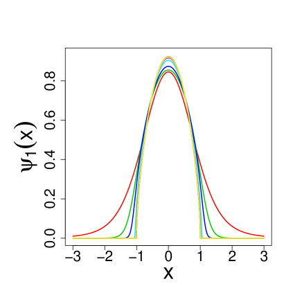
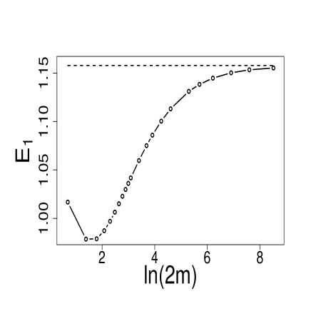
Figure 1: Left panel: $L^{2}(R)$-normalized ground state functions of $\hat{H}=|\Delta|^{1/2}+x^{2m}$ for $m=10$ (red), $50$ (green), $250$ (blue), $2500$ (yellow) and the best-fit infinite Cauchy well eigenfunction (black/yellow) of Ref. zaba1 , c.f. Eq. (47) with $\alpha=1$. Right panel: The bottom eigenvalue dependence on $2m$. The dashed line sets the energy level corresponding to the infinite Cauchy well eigenvalue $E_{1}\sim 1.1578$.

III.3 Reverse engineering: Langevin alternative.

For each $m\geq 1$ let there be given $\rho_{*}(x)=\psi_{1}^{2}(x)$, where $\psi_{1}(x)$ is the $L^{2}(R)$-normalized positive-definite ground state function of the superharmonic Hamiltonian $\hat{H}=|\Delta|^{1/2}+x^{2m}$. As we know, $\psi_{1}(x)=\rho^{1/2}_{*}(x)$ determines the stationary probability density $\rho_{*}(x)=\psi^{2}_{1}(x)$ of a Markovian stochastic process, obeying the principle of detailed balance. The pertinent random dynamics can be recovered by following the non-Langevin approach of Section II.

On the other hand, given the very same stationary pdf $\rho_{*}(x)$, we may attempt a reconstruction of the Langevin system, subject to the Cauchy noise, that would yield a relaxation of any suitable $\rho(x,t)$ to $\rho_{*}(x)$ (here considered as a pre-specified ”target”, eliazar ). We point out that for Langevin-driven Lévy processes the condition of detailed balance generically does not hold true, balance ; balance1 , while being valid in the non-Langevin case.

To quantify relaxation properties of a Markovian Lévy-Langevin process, we need to resort to Eqs. (6) and (7). Actually, to recover the appropriate fractional Fokker-Planck evolution $\partial_{t}\rho=-\nabla(b\cdot\rho)-|\Delta|^{1/2}\rho$ of any suitable $\rho(x,t)$, we must reconstruct the functional form of the drift function $b(x)$. Its functional form must be compatible with the assumption that the chosen target $\rho_{*}(x)$ is a stationary solution of the Cauchy F-P equation.

This amounts to evaluating (in Ref. eliazar an alternative drift reconstruction procedure has been proposed, realized on the level of Fourier transforms)

$$b(x)=-{\frac{\int|\Delta|^{1/2}\rho_{*}(x)\,dx}{\rho_{*}(x)}}\,.$$ (50)

The indefinite integral is to be numerically handled, since we know a priori the functional shape of $\rho_{*}(x)$ (numerical data are in hands). See e.g. gar0 for a couple of analytically accessible examples.

The integration procedure is straightforward. Given $\psi_{1}(x)$, we evaluate point-wise the target pdf $\psi_{1}^{2}(x)=\rho_{*}(x)$. Next we evaluate numerically (c.f. zaba ; zaba1 $|\Delta|^{1/2}\rho_{*}(x)$. Since we know that with the growth of $m$, $\rho_{*}(x)$ decays rapidly beyond the interval $[-1,1]$ (c.f. Fig. 1), and likewise $|\Delta|^{1/2}\rho_{*}(x)$, the indefinite integral of the form $\int f(t)dt$ is actually computed as a definite one $\int_{a}^{x}(f(t)dt$, where the finite lower integration bound $a<-1$ replaces the ”normal” $-\infty$ in the integral.

The outcome of computations if displayed in Fig.2, where all depicted figures derive from the ground state function $\psi_{1}(x)$ of the Cauchy operator $\hat{H}=|\Delta|^{1/2}+x^{2m}$, where $m>1$. For comparison, we depict the drift for the Brownian motion in the interval (equivalently - infinite well) with inaccessible boundaries, gar4 ; brownian , where $b(x)=-\pi\tan(\pi x/2)$ and $\psi_{1}(x)=\cos(\pi x/2)$ on $[-1,1]$. The corresponding random motion belongs to the category of taboo processes, see gar4 ; gar5 ; brownian . In Ref.brownian a comparative discussion can be found, of affinities and the incongruence of Brownian motion scenarios in the infinite well enclosures, in case of (i) absorbing boundaries (Dirichlet), (ii) boundaries inaccessible from the interior (taboo version of Dirichlet data), or (iii) impenetrable, internally reflecting (Neumann).

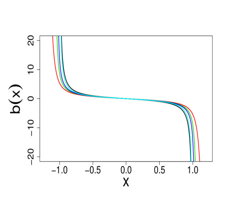
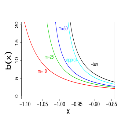
Figure 2: Forward drift of the fractional (Cauchy) Fokker-Planck evolution. Left panel: a couple of $b(x)$ curves is depicted. Details are displayed in the right panel: $m=10$ (red), $m=25$ (green), $m=50$ (blue), $approx$ (turquoise) derives from the best-fit approximate formula for $\psi_{1}(x)$ in the infinite well, Eq. (47) for $\alpha=1$, while $-tan$ (black) refers to the forward drift of the Brownian motion in the infinite well (interval) with inaccessible boundaries (named Brownian taboo process), gar4 .

IV Superharmonic Cauchy-Langevin systems, their non-Langevin partners and ”impenetrable boundaries”.

IV.1 Superharmonic approximation of the Cauchy process in the interval (Langevin realization).

While departing from the Langevin picture of Cauchy flights, which are confined by superharmonic potentials $U(x)=x^{2m}/2m,m\geq 1$ one arrives at the $2m$ sequence of fractional Fokker-Planck equations, whose stationary solutions can be obtained in a closed analytic form. To stay in conformity with Refs. dubkov ; dubkov1 we use the notation $U(x)$ instead of $V(x)$, in the specific context of Langevin-F-P drift fields $b(x)\sim-\nabla U$. The notation $V(x)$, and likewise ${\cal{V}}(x)$, is reserved exclusively for Feynman-Kac potentials and delineated by them ”potential landscapes”.

The formal limiting behavior of the pertinent $2m$-sequence, as $m\rightarrow\infty$, appears to be interpreted in conjunction with the concept of reflected Lévy flights in the interval, denisov ; dubkov ; dubkov1 . This interpretation basically stems from a suggestive large $m$ behavior of a superharmonic sequence of standard Fokker-Plack equations (for superharmonic, drifted Brownian motion), c.f. brownian ; dubkov ; dubkov1 and a semiclassical view of what a dynamics in the infnite well should possibly look like, with a traditional picture of a reflecting ball moving with a uniform velocity between the impacts at interval endpoints (reflecting walls).

The reasoning of Refs. dubkov ; dubkov1 employs the Langevin-type equation $\dot{x}=b(x)+B^{\alpha}(t)$ with a deterministic term $b(x)=-\nabla U(x)=-x^{2m-1},m\geq 1$ and the additive Lévy ”white noise” term. This leads to a fractional Fokker-Planck equation (fogedby , governing the time evolution of the pdf $\rho(x,t)$ of the relaxation process: $\partial_{t}\rho=-\nabla(b\cdot\rho)-|\Delta|^{\alpha/2}\rho$.

In Refs. dubkov ; dubkov1 , for a particular choice of the Cauchy noise ($\alpha=1$), an explicit form of the stationary solution has been derived for all values of $m>2$. A formal $m\to\infty$ limit allows to reproduce the Cauchy version of the steady-state solution for ”Lévy flights in a confined domain”, denisov , where actually it is considered as ”the case of stationary Lévy flights in an infinitely deep potential well”. Since it is claimed by the Authors, that under the infnite well ”confined geometry” conditions, ”the origin of the preferred concentration of flying objects nears the boundaries in nonequilibrium systems is clarified”, we point out our observations to the contrary, c.f. Section III and kwasnicki ; zaba ; zaba1 ; brownian .

Remark 5: We point out that in the original notation of Ref. dubkov ; dubkov1 , it is $p_{st}(x)$ which stands for our $\rho_{*}(x)$. To simplify calculations, we scale away a parameter $\beta$ in the formulas (21), (22) of Ref. dubkov1 (this amounts to setting $\beta=1$). In the original formulas of Ref. dubkov1 , the pertinent parametr $\beta$ comprises $m$ and the interval half-length $L$ in the proportionality factor: $\beta\sim L^{2m/2m-1}$. As $m\to\infty$, we have $\beta\to L$. In the present paper we set $L=1$ and so preselect the interval $[-1,1]$ as a support for the limiting distribution.

For odd values of $m=2k+1$ we have dubkov1 the following expression for the stationary solution $\rho_{*}(x)$ of the superharmonic fractional Fokker-Planck equation:

$$\rho_{*}(x)={\frac{1}{\pi(x^{2}+1)}}\prod_{l=0}^{k-1}{\frac{1}{x^{4}-2x^{2}cos[\pi(4l+1)/(4k+1)]+1}}$$ (51)

while for even values of $m=2k$, we have:

$$\rho_{*}(x)={\frac{1}{\pi}}\prod_{l=0}^{k-1}{\frac{1}{x^{4}-2x^{2}cos[\pi(4l+1)/(4k-1)]+1}}.$$ (52)

A representative sample of pdf shapes $\rho_{*}(x)$ for low values of $m\geq 5$ is depicted in Fig. 3, while a sample of square root pdfs $\rho_{*}^{1/2}(x)$ for larger (medium-sized) superharmonic exponents ($m=10$ to $m=100$) is displayed in Fig. 4.

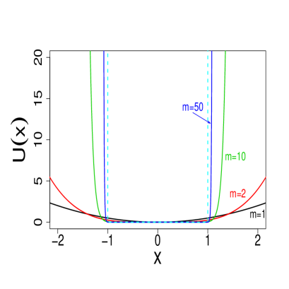
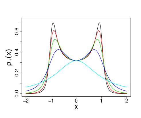
Figure 3: Left panel: The superharmonic potential $U(x)=x^{2m}/2m$ is depicted for $m=1,2,10,50$. The dotted line indicates the shape of the infinitely deep well potential, supported on the interval $[-1,1]$ with the bottom energy level equal zero. We note that $U(\pm 1)=1/2m$ goes to zero as $m\to\infty$. Right panel: We depict stationary pdfs $\rho_{*}(x)$ of the (Langevin-induced) superharmonic Cauchy - Fokker-Planck equation, for $m=1$ (turquois), $2$ (blue), $3$ (green), $4$ (red), $5$ (black).

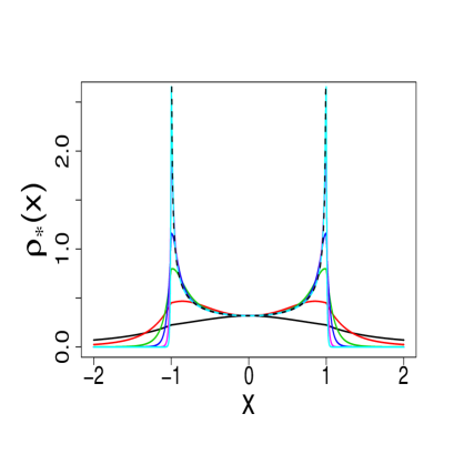
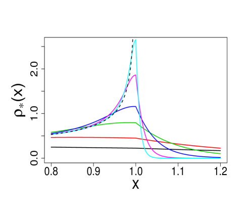
Figure 4: Left panel: Superharmonic stationary probability densities $\rho_{*}(x)$ are depicted for $m=1,2,5,10,25,50$ (indices correspond to consecutive maxima in the growing sequence). The dotted line indicates the arcsine pdf $\rho_{*}(x)[m\to\infty]=1/\pi\sqrt{1-x^{2}}$, which ”lives” exclusively within the open interval $(-1,1)$ and is undefined (actually does not exist) at $\pm 1$ . Right panel: enlarged vicinity of the endpoint $x=1$. Locations of maxima (for each m-th pdf) relative to the arcsine curve, are clearly displayed: they are bounded from above by this curve. The latter is not en envelope, since for all finite $m>1$ we encounter two intersection points at every arcsine branch.

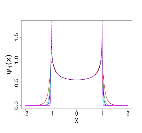
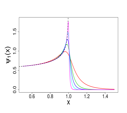
Figure 5: Left panel: $\psi_{1}(x)\equiv\rho_{*}^{1/2}(x)$ for $m=10,20,30,50,100$. Indices correspond to consecutive maxima in the growing order. Right panel: enlarged vicinity of $x=1$. For large values of $m$ (say $m\geq 100$), within the adopted graphical resolution limits, shapes of superharmonic ground states functions are practically indistinguishable from the square root of the arcsine law: $\rho_{*}^{1/2}[m\to\infty](x)\sim(1-x^{2})^{-1/4}$, depicted by a dotted line. Compare e.g. dubkov1 ; dybiec ; denisov .

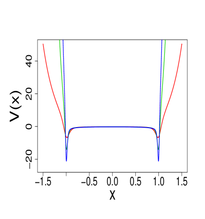
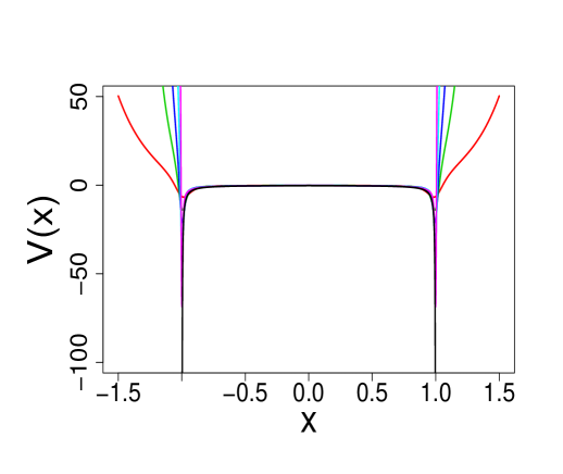
Figure 6: Both panels depict the potential ${\cal{V}}(x)=-\rho_{*}^{-1/2}(x)|\Delta|^{1/2}\rho_{*}^{1/2}(x)$, with $m$-labels and colors shared with Figs. 5 and 7. Left panel: for $m=10$ (red), $20$ (green), $30$ (blue). Right panel: $m=50$ (turquois) and $100$ (pink) are additionally inserted, compare e.g. Fig. 7.

IV.2 Large $m$ behavior: boundary jeopardies.

Let us take advantage of the rearrangement of formulas (51), (52), deduced in the Appendix of Ref. dubkov1 , which explicitly captures the near-boundary behavior in the interval $[-1,1]\subset R$. (The derivation is formal under a presumption that no obstacles come from infinite summations).

We have the following expression for the $2m$-th pdf (the original formula refers to the interval $[-L,L]$ and has more clumsy form in view of the presence of dimensional constants):

$$\rho_{*}(x)={\frac{1}{\pi}}\exp\left\{\sum_{l=1}^{\infty}{\frac{x^{2l}}{2l\cos[\pi l/(2m-1)]}}\right\}$$ (53)

in the interior $(-1,1)$ of the interval of interest (we note that originally dubkov1 the statement was ”for $|x|\leq 1$”, hence referred to the endpoints of the interval as well). The formula valid in the exterior of the interval (originally ”for $|x|>1$”) reads:

$$\rho_{*}(x)={\frac{1}{\pi x^{2m}}}\exp\left\{\sum_{l=1}^{\infty}{\frac{1}{2lx^{2l}\cos[\pi l/(2m-1)]}}\right\}.$$ (54)

Let us analyze point-wise the large $m$ behavior of the definition (53), (54) (to be considered jointly on $R$) of the $2m$-th pdf $\rho_{*}(x)$. First let us notice that (53) and (54) actually coincide at endpoints $\pm 1$ of the interval of interest, provided the series converge. This is the case for all finite values of $m$. However $\rho_{*}(\pm 1)$ diverges in the $m\to\infty$ limit, which is the property of both expressions (53), (54).

Let us assume that $|x|>1$. For all finite values of $m$ the large $m$ behavior of Eq. (54) is ruled by the factor $1/x^{2m}$. Hence for all $|x|>1$, $\rho_{*}(x)$ (and likewise $\rho_{*}^{1/2}(x)$ rapidly drops down to zero as $m\to\infty$. Compare e.g. Figs. 3 and 4.

For all $|x|<1$ the infinite series in the exponent of Eq. (53) converge to finite values, producing function shapes of Figs. 3 and 4, with a visually persuasive $m$-dependence, showing symptoms of the convergence to the arcsine distribution (alternatively, its square root). This feature deserves a more detailed examination.

To this end, presuming $|x|<1$, let us pass to the (formal) $m\to\infty$ limit in the exponent of Eq. (53). We realize that:

$$\rho_{*}(x)_{m\to\infty}={\frac{1}{\pi}}\exp\left\{{\frac{1}{2}}\sum_{l=1}^{\infty}{\frac{x^{2l}}{l}}\right\}.$$ (55)

The series in the exponent can be summed by invoking the Taylor expansion of the function $\ln(1-z)=-(z+z^{2}/2+z^{3}/3+...)$, which upon substitution $z\rightarrow x^{2}$ gives rise to the arcsine distribution in $(-1,1)$:

$$\rho_{*}(x)_{m\to\infty}={\frac{1}{\pi}}\exp[-{\frac{1}{2}}\ln(1-x^{2})]={\frac{1}{\pi\sqrt{1-x^{2}}}}.$$ (56)

We note that the arcsine distribution has been here associated exclusively with the interior $(-1,1)$ of the interval $[-1,1]$, with endpoints (and the whole exterior of $[-1,1]$ in $R$0 excluded from consideration. The pertinent distribution diverges as we approach $\pm 1$.

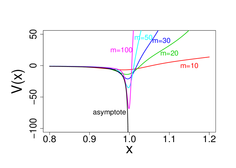
Figure 7: The enlargement of the vicinity of $x=1$ in Fig. 6 clearly shows a surprising affinity (approximation finesse in the range ${\cal{V}}(x)\leq 0$) set against a coexisting dramatic difference (in the vicinity of the interval endpoints) between overall shapes of ${\cal{V}}(x)$ for finite (albeit arbitrarily large) values of $m$ and the shape of the ”asymptote” ${\cal{V}}(x)[m\to\infty]$ (black), which is reconstructed from $\rho_{*}^{1/2}(x)[m\to\infty]$, Eq. (57).

IV.3 Non-Langevin approach: Cauchy-Schrödinger semigroup and its equilibrium state.

In accordance with arguments of Section II, the non-Langevin approach amounts to the reconstruction of the dynamics from the ground state function of a suitable fractional energy operator (fractional Hamiltonian). We have in hands the Langevin-FP induced superharmonic stationary densities. These are supposed to be shared by the non-Langevin alternative as well.

The $m$-labeled ground state functions are numerically inferred by taking the square root of the $m$-th stationary pdf: $\psi_{1}(x)=\rho_{*}^{1/2}(x)$ and depicted in Fig. 5. We note that, like in Fig. 4, all maxima of superharmonic functions (pdfs and their square roots) are located below the arcsine curve and its square root, correspondingly. The arcsine curves cannot be considered as envelopes of superharmonic function families since, generically in each branch, they have two intersection points (hence no tangent point) with each superharmonic one. Nonetheless, for large values of $m$, their rough interpretation as fapp envelopes is surely admissible (”fapp” abbreviates ”for all practical purposes”).

To infer the Feynman-Kac (landscape) potentials ${\cal{V}}(x)$, in accordance with the discussion of Section II, we rely on the numerically assisted procedure as well. Its workings (specifically on how to handle effects of integration cutoffs) have been tested before, gar ; gar1 ; zaba ; zaba1 ; gar0 ; gar2 , see also gar5 and brownian . Given $\psi_{1}(x)$, we numerically evaluate the integral (5), while adjusted to the Cauchy case $-(|\Delta|^{1/2}\psi_{1})(x)$, and point-wise divide the outcome by $\psi_{1}(x)$, so arriving (point-wise again) at the resultant ${\cal{V}}(x)$.

The Feynman-Kac potentials ${\cal{V}}(x)$, inferred from a priori given $m$-sequence $\psi_{1}(x)$, are depicted in Figs. 6 and 7. In the right panel of Fig.6, and its enlargement in the vicinity of $x=1$, displayed in Fig. 7, the black curve depicts the potential shape ${\cal{V}}[m\to\infty](x)$, obtained by adopting the general reconstruction recipe (c.f. Eq. (27)), to the square root of the formal asymptotic ($m\to\infty$) steady state Cauchy solution $\rho_{*}(x)$, Eq. (57) and dubkov1 .

Following our non-Langevin reconstruction principles of Section II, we infer the Hamiltonian $\hat{H}=|\Delta|^{1/2}+{\cal{V}}(x)$, whose ground state eigenfunction ($m\to\infty$ indication is formal, the convergence is not uniform)

$$\rho^{1/2}_{*}(x)_{m\to\infty}={\frac{1}{\sqrt{\pi\sqrt{1-x^{2}}}}}$$ (57)

is associated with zero eigenvalue. To this end, we have numerically computed the corresponding ${\cal{V}}(x)$, see e.g. Figs. 6 and 7. Note an excellent (within graphical resolution limits) approximation of superharmonic potential profiles by an asymptote (57), delineated in black in Figs. 6 and 7, in the open interval $(-1,1)$. The behavior of superharmonic potential profiles at the close vicinity of interval endpoints is drastically different (violent decay followed by violent growth, c.f. the case of $m=50$ and $m=100$ in Fig. 7) from the monotonic decay of the curve (57) towards minus infinity at both endpoints $\pm 1$ of the interval.

The black-colored curve in Figs. 6 and 7 delineates the potential, which is entirely confined in the interval $[-1,1]$. The potential is non-positive, with branches rapidly escaping to $-\infty$ at the interval endpoints. To the contrary, the superharmonic profiles ultimately escape to $+\infty$, while approaching $\pm 1$.

Making a naive, but straightforward comparison with the inverted harmonic oscillator potential, we realize that the problem refers to the scattering phenomena in the interval $(-1,1)$. Here, one needs an additional information (absent in the formal definition of the pertinent ${\cal{V}}(x)$) that the scattering is actually limited by impenetrable walls at $\pm 1$.

It seems that we have nothing to say about the well (interval) exterior in $R$. However, we shall demonstrate that actually one cannot disregard the exterior $R\setminus(-1,1)$ of the interval $(-1,1)$, in any discussion of confined Lévy processes. It has been the case for Dirichlet enclosures of Section III, and appears to be a general feature of nonlocal generators of Lévy flights in ”confined geometries”.

V Meaning of ”confined geometry”, confined domain” and ”infinitely deep well” in the context of Lévy flights.

In the statistical physics literature, the ”infinitely deep potential well” is typically considered as a model of a ”confined domain” with impermeable boundaries denisov , and thence intuitively associated with reflected random motions that never leave the prescribed enclosure. This happens both in the context of Lévy flights dubkov1 -trap , and in case of the standard Brownian motion dubkov1 ; brownian . This presumption is conceptually amplified by reference to the semiclassical relative of the (quantum) infinite potential well, visualized by a mass point in uniform motion, which is perpetually reflecting from rigid walls.

However, the ”reflecting walls” association is somewhat misleading and stays in plain conflict with our observations of Section III (see also a sample of related references). Indeed, there are other random processes which relax to equilibrium in a finite enclosure, and definitely have not much in common with the reflection scenario, gar ; gar5 . Some of them refer to so-called taboo processes, where the (originally) absorbing boundaries turn over into inaccessible ones. The exterior Dirichlet boundary conditions are here implicit and their workings were briefly outlined in Section III. The corresponding Lévy relaxation processes have been discussed in Section II.

In Refs. denisov ; dubkov1 , explicitly dealing with Lévy flights in the ”infinitely deep potential well”, no link has been established with the fractional Laplacian subject to any form of Neumann boundary data (presumably nonlocal). Hence, the notion of a valid generator of the Lévy process in a bounded domain with reflecting boundaries appears to be absent (and basically remains an open question gar5 ).

Remark 6: The issue of reflected Lévy flights is not a novelty in the mathematical literature, and basically defined through a path-wise (Skorokhod SDE) realization, asm . While passing to motion generators, restricted forms of fractional Laplacians should enre the stage. Here, one encounters ambiguities in the proper formulation of the Neumann-type condition. In the present paper we leave aside a discussion of various approaches to this issue and refer to gar5 ; asm ; valdi ; abat0 ; warma ; guan ; guan1 ; bogdan0 ; bogdan . We point out that so called regional fractional Laplacians have been identified as generators of reflected Lévy processes in Ref. guan ; guan1 , see also bogdan for a discussion of censored Lévy flights.

In Ref. denisov , by departing from the Langevin-Fokker-Planck approach to the study of Lévy flights in the ”infinitely deep potential well”, the analytic formula for steady states has been derived: ”it is shown that Lévy flights are distributed according to the beta distribution, whose probability density becomes singular at the boundaries of the well. The origin of preferred concentration of flying objects near the boundaries in nonequilibrium systems is clarified”. (In passing, we mention that the arcsine distribution (56) is a member of the above beta pdfs family, dubkov1 .)

The above statement needs to be kept under scrutiny, since the infnite well enclosure is known to admit Dirichlet boundaries which are inaccessible. The boundary value zero for functions in the domain of the Dirichlet fractional Laplacian is approached continuously (there is no accumulation of flying objects near the boundary, they are driven away). An obvious conflict of the probability accumulation statement, with a plentitude of results obtained for Lévy flights in the Dirichlet well (see Section III and references cited therein), makes tempting to inquire into the roots of this incongruence. We shall comparatively address this issue in below.

V.1 How does the steady-state distribution of Lévy flights derive under the infinite well conditions: The argument of Ref. denisov .

In Ref. denisov , the departure point is a formal Langevin equation $\dot{x}(t)=f(x(t),t)+\xi(t)$ where $f(x,t)=-\nabla U(x,t)$ is a force field, $U(x)$ an external deterministic potential, and $\xi(t)$ stands for the Lévy ”white noise”. Ways to handle the formal ”noise” term , and derive an associated fractional Fokker-Planck equation, have been described in denisov , see also fogedby . The Authors prefer to employ the Riemann-Liouville derivatives, which in case of the symmetric Lévy stable noise imply a familiar fogedby expression for the Lévy Fokker-Planck equation for a time dependent probability distribution $\rho(x,t)$:

$${\frac{\partial\rho(x,t)}{\partial t}}=-{\frac{\partial[f(x,t)\rho(x,t)]}{\partial x}}+\gamma{\frac{\partial^{\alpha}\rho(x,t)}{\partial|x|^{\alpha}}},$$ (58)

where $\gamma$ stands for the ”noise” intensity parameter (to be scaled away), while the fractional derivative conforms with our previous notation, according to: $|\Delta|^{\alpha/2}\rho(x,t)=-\partial^{\alpha}\rho(x,t)/\partial|x|^{\alpha}$, $0<\alpha<2$.

The ”confined geometry” of the infinitely deep potential well is created by demanding: (i) $f(x,t)=0$ within the well, i.e. for $x\in[-L,L]$, where $2L$ is the width of the well, (ii) boundaries at $x=\pm L$ are impermeable, i. e. $\rho(x,t)=0$ for $|x|>L$; this restriction tacitly presumes that the term $f(x,t)\cdot\rho(x,t)$ may be safely discarded if $|x|>L$, while nothing is said about what actually $f(x,t)$ outside the well is.

The subsequent conclusion of denisov reads: ”with these conditions the [fractional Fokker-Planck] equation for the stationary probability density $\rho_{*}(x)$ reduces to” (here, we employ the notation of Eq. (58)):

$$|\Delta|^{\alpha/2}\rho_{*}(x)=0,$$ (59)

where $\rho_{*}(x)=0$ for $|x|>L$, and nothing is said about the (non)existence or specific values taken by $\rho_{*}(x)$ at boundary points $x=\pm L$ .

Presuming that the fractional Fokker-Planck equation (58) and likewise its stationary variant (59), can be (in the least formally) rewritten in the divergence form $\partial_{t}\rho(x,t)=-\nabla j(x,t)$ where $j(x,t)$ is interpreted as a probability current. Accordingly (59), while presented in the time-independent form $\nabla j(x)=0$, says that $j(x)=const$. At this point a boundary condition upon the probability flow intervenes: (iii) $j(\pm L)=0$, whose consequence is $j(x)=0$ for all $x\in[-1,1]$. A hidden assumption is that $j(x)$ may be continuously interpolated up to the boundaries, while $\rho_{*}(x)$ may not.

Remark 7: A formulation of the fractional analog of the Fick law is subtle, and likewise an inversion $\nabla^{-1}$ of the gradient operator is a subtle matter. This cannot be considered a priori granted, and the procedure may fail in some stability parameter $\alpha$ ranges, c.f. neel ; gar7 . Then, the notion of a (fractional) probability current cannot be introduced at all.

Conditions (i)-(iii) suggest the functional trial form of the sought for solution, and the subsequent computation, while restricted to symmetric Lévy flights ($0<\alpha<2$) in the well, ends up with the $\alpha$-family of probability density functions in $(-1,1)$, which escape to $+\infty$ while approaching the interval endpoints $\pm L$:

$$\rho_{*}(x)=(2L)^{1-\alpha}\,{\frac{\Gamma(\alpha)}{\Gamma^{2}(\alpha/2)}}(L^{2}-x^{2})^{\alpha/2-1}.$$ (60)

For the Cauchy noise $\alpha=1$, and with the choice $L=1$ of the interval length parameter, we arrive at the arcsine law in the form (56).

V.2 Boundary data issue.

Our notational convention of Section I.A gives preference to the nonegative operator $|\Delta|^{\alpha/2}$, while one should keep in memory that it is $-|\Delta|^{\alpha/2}=-(-\Delta)^{\alpha/2}$ which is a valid fractional relative of the ordinary Laplacian $\Delta$. With reference to the normalization coefficient ${\cal{A}}_{\alpha}$ our version (c.f. Eq. (5)) is specialized to one spatial dimension and ultimately to the Cauchy case $\alpha=1$.

To avoid confusion, we recall an often employed definition of the symmetric Lévy stable generator in $R^{n}$, in the integral form which involves an evaluation of the Cauchy principal value (p.v.). For a suitable function $f(x)$, with $x\in R^{n}$ and $n\geq 1$, we have:

$$|\Delta|^{\alpha/2}f(x)=(-\Delta)^{\alpha/2}f(x)=\mathcal{A}_{\alpha,n}\lim\limits_{\varepsilon\to 0^{+}}\int\limits_{{R}^{n}\supset\{|y-x|>\varepsilon\}}\frac{f(x)-f(y)}{|x-y|^{\alpha+n}}dy,$$ (61)

where $dy\equiv d^{n}y$ and the (normalization) coefficient

$$\mathcal{A}_{\alpha,n}=\frac{2^{\alpha}\Gamma({\frac{\alpha+n}{2}})}{\pi^{n/2}|\Gamma(-{\frac{\alpha}{2}})|}=\frac{2^{\alpha}\alpha\Gamma({\frac{\alpha+n}{2}})}{{\pi^{n/2}\Gamma(1-\alpha/2})}$$ (62)

is adjusted to secure the conformity of the integral definition (61) with its Fourier transformed version. The latter actually gives rise to the Fourier multiplier representation of the fractional Laplacian, c.f. gar7 ; abat , ${\cal{F}}[(-\Delta)^{\alpha/2}f](k)=|k|^{\alpha}{\cal{F}}[f](k)$. If the fractional operator (61) is defined on $R$, the coefficient (62) can be recast in the form, made explicit in Eq. (5).

Let us assume to have given a function $f(x)$, defined on the whole of $R$, which has the form $f(x)=u(x)=(1-x^{2})^{-1+\alpha/2}$ for $x\in(-1,1)$ and vanishes outside of the open interval $(-1,1)$, e.g. $f(x)=0$ for $x\in R\setminus(-1,1)$. Thus, our function is presumed to vanish both at the boundary points (endpoints) $\pm 1$ and beyond $[-1,1]$ as well.

The computational outcome of Ref. dyda reads $|\Delta|^{\alpha/2}u(x)=0$ for all $x\in(-1,1)$. An analogous outcome is obtained for functions $v(x)=xu(x)$. There holds $|\Delta|^{\alpha/2}v(x)=0$ as well, for all $x\in(-1,1)$. Functions that remain constant in $D=(-1,1)$ and vanish in $R\setminus D$, are valid elements of the (domain) kernel of the operator $|\Delta|^{\alpha/2}$ as well.

The Cauchy case refers to $\alpha=1$, and the arcsine law (56), while extended to the whole $R$, as a function identically vanishing on the complement of $(-1,1)$ provides an example of the above introduced function $u(x)$.

Remark 8: We point out that the computation of eigenfunctions and eigenvalues of the (Cauchy) fractional Laplacian with exterior Dirichlet boundary conditions (e.g. that in the ”infinite potential well”), c.f. Section III.C of ref. zaba1 , makes an explicit usage of the assumption that the (bounded) eigenfunctions $\psi(x)$ of $|\Delta|^{1/2}$ continuously approach the value $0$, while reaching the endpoints $\pm 1$ of $[-1,1]$ from the its interior $(-1,1)$. C.f. Eqs. (5)-(7) and (47) in Ref. zaba1 , where this demand is explicitly stated

$$\lim_{x\to\pm 1}|\Delta|^{1/2}\psi(x)=0,$$ (63)

for solutions of the eigenvalue problem $|\Delta|^{1/2}\psi(x)=\lambda\,\psi(x)$, with $\lambda\geq 0$ (actually $\lambda>0$ in the exterior Dirichlet enclosure, kulczycki -zaba3 ).

It is the condition (63) which makes a crucial difference between two ”infinitely deep well” cases discussed in the present paper: this described in Section III respects (64), while this outlined in the present Section, following Ref. denisov , does not. The difference is evidenced in the boundary properties of functions depicted in Fig. 1 (convergence to $0$) and the divergence of steady state pdfs (46) and (60), as depicted in Fig. 4. We shall come back to this point in below, by means of analytic arguments.

V.3 Singular $\alpha$-harmonic functions.

Since functions (56) and (60) may be interpreted as solutions of the fractional Laplacian eigenvalue problem with the eigenvalue zero, we have here a natural link with the concept of singular $\alpha$-harmonic functions bogdan ; ryznar and closely related blow-up phenomena for ”large solutions” of fractional elliptic equations abat -vazquez . An inspection of Fig. 4 reveals another link, with the concept of locally accurate approximations to ”almost every function”, which are provided by suitable $\alpha$-harmonic ones.

In the Cauchy context, we have an explicit statement, ryznar concerning the concept of $\alpha$-harmonicity. Let $\alpha<2$, and suppose that $D$ is an open unit ball in $R^{n}$. Then, the function $f(x)=(1-|x|^{2})^{\alpha/2-1}$ for $|x|<1$ and $f(x)=0$ for $|x|\geq 1$ is $\alpha$-harmonic in $D$ and $\lim_{x\to Q\in\partial D}=\infty$. Here $Q$ refers to points of the boundary $\partial D$ of $D$ (i.e. interval endpoints if $n=1$ and $D=(-1,1)$).

According to Refs. bogdan0 ; bogdan1 : (i) a function $f$ is singular $\alpha$-harmonic in an open set $D$ if it is $\alpha$-harmonic in $D$ and $f(x)=0$ for $x\in D^{c}=R^{n}\setminus D$; (ii) a function $f$ is $\alpha$-harmonic in $D$ if and only if it is $C^{2}$ on $D$ and $|\Delta|^{\alpha/2}f(x)=0$ for all $x\in D$.

It is (ii), which directly refers to our previous discussion. We emphasize that for (ii) to hold true, the function $f(x)$ must be defined on the whole of $R^{n}$. The values of $f(x)$ on $D^{c}$ are indispensable for this property and must not be disregarded (or ignored). This reflects the fact that the fractional Laplacian is a nonlocal operator and without special precautions bogdan ; gar5 there is no way to eliminate a direct influence (e.g. jumps) between distant points $x$ and $y$ in the domain of $f$.

On the other hand, the notion of $\alpha$- harmonicity can be introduced in the purely probabilistic lore, with direct reference to Lévy flights, thus providing hints toward computer-assisted path-wise procedures, yielding the singular $\alpha$-harmonic functions as would-be steady states of Lévy flights in the (appropriately defined) ”infinite potential well”, dubkov1 ; dybiec ; denisov .

To this (probabilistic/stochastic) end, c.f. bogdan0 ; bogdan1 , we employ the notion of the first exit time from $A\subset R^{n}$ (alternatively, first entrance time to $A^{c}=R^{n}\setminus A$) of the isotropic $\alpha$-stable Lévy process $X_{t}$. Given the Borel set $A$, we define $\tau_{A}=\inf\{t\geq 0:X_{t}\in A^{c}\}$ as the first exit time from $A$. For a bounded set $A$, we have $\tau_{A}<\infty\,\,a.s.$. We define a local expectation value

$$u(x)=E^{x}u(X_{\tau_{A}})=E^{x}[u(X_{\tau_{A}});\,\tau_{A}<\infty],$$ (64)

interpreted as an average taken at random (exit/entrance) time $\tau_{A}$ values, with respect to the process $X_{t}$ started in $x$ at $t=0$, with values $X_{t}=y\in A$.

For a Borel measurable function $u\geq 0$ on $R^{n}$, we say that:
(i) $u(x)$ is regular $\alpha$-harmonic in an open set $A\subset R^{n}$, if $u(x)=E^{x}[u(X_{\tau A})]<\infty$, $x\in A$;
(ii) $u(x)$ is $\alpha$-harmonic in $A$, if for every bounded open set $B$ with the closure $\overline{B}$ contained in $A$ we have $u(x)=E^{x}[u(X_{\tau B})]<\infty$, $x\in B$;
(iii) $u(x)$ is singular $\alpha$-harmonic in $A$, if $u(x)$ actually is $\alpha$-harmonic in $A$ and $u(x)=0$ for all $x\in A^{c}$.

Accordingly, the ”steady state functions” (56) and (60), while interpreted as valid solutions of Eqs. (63) and (59) respectively (and thus complemented by the exterior boundary condition), are examples of singular $\alpha$-harmonic functions in $D=(-1,1)$.

We note that a visual inspection of both panels in Fig. 4 clearly indicates that, while in $(-1,1)$, the singular $\alpha$-harmonic function $\rho_{*}(x)$ may be considered as a perfect approximation of large $m$ superharmonic pdfs. (This property stays in conformity with recent Ref. valdi1 , according to which ”all functions are locally $\alpha$-harmonic up to a small error”.)

In the exterior of $[-1,1]$ i.e. for $x>1$, the pertinent pdfs, in the large $m$ regime, rapidly decay to zero. The behavior (with $m\to\infty$) of these pdfs is subtle: we have (i) growth to $\infty$ for $|x|\leq 1,|x|\uparrow 1$, and (ii) decay to zero for $|x|\geq 1,|x|\downarrow 1$.

V.4 Domain intricacies and the relevance of exterior contributions.

A formal statement of the exterior Dirichlet boundary data for the fractional operator (negative fractional Laplacian) $|\Delta|^{\alpha/2}$ may be condensed in the notion of the elliptic problem, warma : $|\Delta|^{\alpha/2}u=f$ in $\Omega$ and $u=0$ in $R^{n}\setminus\Omega$ where $\Omega\subset R^{n}$ is an arbitrary bounded open set. Actually, this is a departure point for the study of the eigenvalue problem $|\Delta|^{\alpha/2}u=\lambda u$, provided $|\Delta|^{\alpha/2}$ has a realization in $L^{2}(\Omega)$, e.g. both $u$ and $f$ are elements of $L^{2}(\Omega)$. The eigenvalues $\lambda$ are known to be positive, $\lambda>0$ , c.f. kulczycki ; kwasnicki ; zaba ; zaba1 .

The Cauchy ($\alpha=1$) version of the pertinent spectral problem, under exterior Dirichlet boundary data, has been briefly summarized in Section III, with the notational replacement of $\Omega$ by $D$.

Right at this point we emphasize, that the singular $\alpha$-harmonic functions (56) and (60) formally correspond to the eigenvalue zero of the fractional Laplacian, while considered in $L(\Omega)$, e.g. not in $L^{2}(\Omega)$. Note that to employ the framework of Section II, we were forced to introduce the square root of the arcsine pdf, (57), to deal with the $L^{2}(\Omega)$ (actually $L^{2}(D)$) setting.

Our further analysis pertains to the Cauchy case. For a while we disregard the domain issues, i.e. $L$ versus $L^{2}$, and/or involved Sobolev spaces, warma , and formally address the existence of solutions of the fractional equation $|\Delta|^{1/2}\rho_{*}(x)=0$ in $D=(-1,1)$, with exterior Dirichlet boundary data in $R\setminus D$, c.f. (59). We know that not only positive solutions are admitted, dyda , and that arbitrary constants do this job as well.

We are interested in an explicit justification of the existence of positive solutions with the blow-up at the boundaries $\pm 1$ of $D^{c}=[-1,1]$. In below we shall analytically demonstrate that the arcsine pdf (56) is an example of a fully-fledged singular $\alpha=1$-harmonic function in $D=(-1,1)$ and indicate: (i) an exterior to $(-1,1)$ input to the solution, and (ii) the role (acceptance or abandonment) of the ”continuity up to the boundary” condition (64).

We depart form the integral definition (4) of the fractional operator $|\Delta|^{1/2}$, where ${\cal{A}}_{1}=1/\pi$. Let us tentatively consider the action of $|\Delta|^{1/2}$ on $C_{0}^{\infty}(R)$ functions $\psi(x)$ supported in $D=(-1,1)$, i.e. such that $\psi(x)=0$ for all $x\in R\setminus D$. We have ($(p.v.)$ means Cauchy principal value):

$$|\Delta|_{D}^{1/2}\psi(x)=-\frac{1}{\pi}(p.v.)\int_{R}\frac{\psi(x+y)-\psi(x)}{y^{2}}dy.$$ (65)

Given $x\in(-1,1)$, we realize that $\psi(x+y)$ does not vanish identically if $x+y\in(-1,1)$ i.e. for $-1-x<y<1-x$. Hence, the integration (65) can be simplified by decomposing $R$ into $(-\infty<y\leq-1-x)\cup(-1-x<y<1-x)\cup(1-x\leq y<\infty)$. Therefore, we end up with a restricted fractional operator:

$$|\Delta|_{D}^{1/2}\psi=-\frac{1}{\pi}\left[-\psi(x)\left(\int_{-\infty}^{-1-x}\frac{dy}{y^{2}}+\int_{1-x}^{\infty}\frac{dy}{y^{2}}\right)+\int_{-1-x}^{1-x}\frac{\psi(x+y)-\psi(x)}{y^{2}}dy\right]=$$

$$=\frac{2}{\pi}\frac{\psi(x)}{1-x^{2}}+\frac{1}{\pi}\int_{-1-x}^{1-x}\frac{\psi(x)-\psi(x+y)}{y^{2}}dy,$$ (66)

where the second integral should be understood as the Cauchy principal value with respect to $0$, i.e. $\int_{-1-x}^{1-x}=\lim_{\varepsilon\to 0}\left[\int_{-1-x}^{-\varepsilon}+\int_{-\varepsilon}^{1-x}\right]$.

We point out that the first term on the right-hand-side of Eq. (66) includes an outcome of the integration over $R\setminus D$, i.e. an input exterior to $D=(-1,1)$ proper. It is instructive to notice that the change the integration variable $y=t-x$ in the second term of Eq. (66) gives rise to

$$|\Delta|_{D}^{1/2}\psi(x)=\frac{2}{\pi}\frac{\psi(x)}{1-x^{2}}+\frac{1}{\pi}\int_{-1}^{1}\frac{\psi(x)-\psi(t)}{(t-x)^{2}}dt,$$ (67)

where the $R\setminus D$ and $D$ contributions are now clearly isolated, albeit the ultimate overall $x$-dependence refers to $x\in D$ only. The Cauchy principal value of the integral in Eq. (67) is no longer evaluated with respect to $0$, but with respect to $x$.

The integral expression in Eq. (67) which is restricted to $t\in(-1,1)$, and $x\in(-1,1)$, is the Cauchy version of the so-called regional fractional Laplacian in $D^{c}=[-1,1]$, bogdan ; warma ; gar5 ; zaba1 .

Our further discussion will be based on the decomposition (66), which has been used in Ref. zaba1 , for the computer-assisted shape analysis of nonolocally induced fractional (Cauchy) bound states in the infnite well. See e.g. Section III of the present paper, and the approximate formula (49) for the ground state function, which reproduces the $\sim\sqrt{1-x^{2}}$ decay to $0$, while approaching the boundary points $\pm 1$ of the interval $(-1,1)$. This, in conformity with the condition (63), and at variance with the boundary blow-up property of (56) and (60).

V.5 Explicit evaluation of the singular $(\alpha=1)$-harmonic function in $(-1,1)$.

In Refs. zaba ; zaba1 , we have assumed that any even eigenfunction of the Dirichlet fractional Laplacian $|\Delta|^{1/2}_{D}$ (given by Eq. (66), restricted by the exterior Dirichlet boundary data to $D$, and additionally by the local boundary condition (63)), should be sought for by analyzing convergence features of consecutive polynomial approximations of $2N,N\to\infty$ degree, in terms of power series expansion (here given up to the normalization coefficient):

$$\psi(x)=\sqrt{1-x^{2}}\sum_{k=0}^{N}\alpha_{2n}x^{2n},\qquad\alpha_{0}=1.$$ (68)

In Ref. zaba1 our major task has been to determine expansion coefficients $\alpha_{2n}$, for sufficiently long series expansion (we have computationally reached $2N=500$).

Given the definition (66) of $|\Delta|_{D}^{1/2}$ restricted to $\psi$’s with support in $D$. Let us formally proceed with its integral part, here denoted

$$I_{D}\psi(x)=\frac{1}{\pi}\int\limits_{-x-1}^{-x+1}\frac{\psi(x)-\psi(x+z)}{z^{2}}dz.$$ (69)

Consider the (formal) action of $I_{D}$ upon functions of the form $\psi(x)=x^{2n}\sqrt{1-x^{2}}$. We get (compare e.g. zaba1 ):

$$I_{D}x^{2n}\sqrt{1-x^{2}}=-\frac{2}{\pi}\frac{x^{2n}\sqrt{1-x^{2}}}{1-x^{2}}+(c_{2n}+3c_{2n-2}x^{2}+5c_{2n-4}+\ldots+(2n+1)c_{0}x^{2n}),$$ (70)

where $c_{2k}$ are expansion coefficients of the Taylor series for $\sqrt{1-x^{2}}$:

$$\sqrt{1-x^{2}}=\sum_{k=0}^{\infty}c_{2k}x^{2k}=\sum_{k=0}^{\infty}\frac{(2k)!}{(1-2k)(k!)^{2}4^{k}}x^{2k}.$$ (71)

We note that

$${\frac{1}{\sqrt{1-x^{2}}}}=(1+x^{2}+x^{4}+...)\sqrt{1-x^{2}}$$ (72)

where we recognize a factor which is a sum of a geometric progression with the ratio $x^{2},|x|<1$. This allows to evaluate term after term (presuming suitable convergence properties of the series) the expression:

$$|\Delta|^{1/2}_{D}{\frac{1}{\sqrt{1-x^{2}}}}=\sum_{n=0}^{\infty}|\Delta|^{1/2}_{D}[x^{2n}\sqrt{1-x^{2}}]=\sum_{n=0}^{\infty}c_{2n}+3x^{2}\sum_{n=0}^{\infty}c_{2n}+5x^{4}\sum_{n=0}^{\infty}c_{2n}+...=0.$$ (73)

Here, we note that the function $\sqrt{1-x^{2}}$ is defined on $[-1,1]$ and takes the value $0$ at $x=\pm 1$. Accordingly, $\sum_{k=0}^{\infty}c_{2k}=0$ and therefore there holds the expected result $|\Delta|^{1/2}_{D}(1-x^{2})^{-1/2}=0$.

We emphasize that in view of (70), the exterior (by origin) term in (66) and (67) is cancelled by the intrinsic (to $D$) counterterm $-2\psi(x)/\pi(1-x^{2})$.

Remark 9: We point out that potentially troublesome issues of the interchange of infnite summations and integrals have been bypassed. To facilitate the passage from (70) to (73), let us indicate that: $|\Delta|^{1/2}_{D}\sqrt{1-x^{2}}=1$, $|\Delta|^{1/2}_{D}x^{2}\sqrt{1-x^{2}}=3x^{2}-1/2$, $|\Delta|^{1/2}_{D}x^{4}\sqrt{1-x^{2}}=5x^{4}-3x^{2}/2-1/8$, $|\Delta|^{1/2}_{D}x^{6}\sqrt{1-x^{2}}=7x^{6}-5x^{4}/2-3x^{2}/8-1/16$ and so on. Summation of these expressions, paralleled by collecting together terms standing at consecutive powers of $x^{2n},n=0,1,2,...$, gives rise to geometric progressions: $x^{0}(1-1/2,-1/8-1/16-...)$, $3x^{2}(1-1/2-1/8-...)$, $5x^{4}(1-1/2-1/8-...)$ etc.

VI Conclusions: Path-wise justification attempts for the relaxation process in the ”confined domain”.

As a brief introduction to subsequent comments, we list simple (Monte Carlo) updating scenarios, which are supposed to to mimic the random path reflection in the two barrier problem (e.g. interval $(-L,L)$ or the infinite well set on this interval), dybiec .

(I)Reversal (wrapping): A trajectory that ends at $x<-L$ is wrapped around the left boundary : $x\to-L+|x+L|$.
(II) Stopping: A trajectory that aims to cross $-L$ is paused (stopped) at $-L+\epsilon$, where $\epsilon>0$ is fixed and small. The point $-L+\epsilon$ is a starting point for the next jump (next in terms of the simulation procedure/time). The barrier is inaccessible to the trajectory.
(III) Superharmonic confinement: The Langevin-type equation with a superharmonic force term $-\nabla U=-x^{2m-1}/L^{2m}$, $2m\gg 2$ is used to simulate the Lévy motion.

A particular property of confined Lévy flights, we have discussed throughout the present paper, is the accumulation (ultimately interpreted as a blow-up) of ”steady state” (or equilibrium) probability density functions (and thence probability) near the boundaries of the confining potential well, c.f. Figs. 3 to 7 and (56), (60). Such phenomena have been reported in computer studies of anomalous diffusions and specifically the fractional Brownian motion, klafter -vojta2 . In the computation, traditional reflection-from-the-barrier path-wise recipes (wrapping scenario) were adopted, in conjunction with steep potential well Langevin models.

Leaving aside the case of the fractional Brownian motion and coming back to the Lévy flights issue, we point out that the path-wise search for a consistent implementation of the reflecting boundary data and the reflection event proper, has been carried out in Refs. dybiec0 ; dybiec ; dubkov1 . Probability density functions were obtained by means of numerical path-wise (Monte Carlo) simulations, based on the Langevin-type equation with the fractional ($\alpha$-stable) ”white noise” term. In fact, stochastic differential equations were numerically integrated by applying the Euler-Maruyama-Ito method, weron . Large numbers of sample trajectories of involved random variables $X(t)$ were generated, which enabled an approximate reconstruction of the pdf $\rho(x,t)$ at a chosen (large) simulation time instant $t$. A stabilization of outcomes (pdf’s shapes) for time instants $t$ large enough, has been interpreted as a symptom of stationarity of the asymptotic stationary pdfs $\rho_{*}(x)$.

In particular, for the superharmonic confinement (case (III)) of $\alpha$-stable Lévy flights, the accumulation near the endpoints of the interval $[1,1]$ has been convincingly confirmed. The interpretation, Ref. dybiec of the binding potential $U(x)=x^{2m}/2m$, $m\gg 1$, has been literally coined as that of a model of the reflecting boundary. Exemplary simulations were executed for $2m=800$. (Other models of would-be reflecting boundaries are present in the literature as well, see e.g. vojta2 .)

On the available graphical resolution level, a high approximation accuracy of singular $\alpha$-stable harmonic functions has been achieved, by means of the stopping scenario (II) for random motions between two impenetrable barriers, dubkov1 ; dybiec .

A serious conceptual obstacle should be mentioned. Namely, if for Lévy flights in the infinite well, we adopt the wrapping (reflection) scenario (I) at the barriers, then irrespective of the stability index $0<\alpha<2$, the estimated (asymptotic) trajectory statistics corresponds to the uniform distribution $1/2$ in $(-1,1)$, c.f. dybiec , see e.g. also gar5 ; brownian .

On the other hand, none of the adopted path-wise reflection scenarios has been ever tested (as useful or useless) in the mathematical research on reflected Lévy flights, developed sofar, asm -bogdan . Interestingly, main efforts were concentrated on the formulation of the fractional (basically nonlocal) analogue of the Neumann condition (as opposed to the exterior Dirichlet one). However, so constrained jump-type process appear not to be confined in the interior of the well, but in principle may reach exterior (beyond the barrier) locations. The ”reflection” is mimicked by the instantaneous return i.e. the jump back to the well interior, with a prescribed jump intensity, valdi ; warma . This is plainly inconsistent with the barrier ”impenetrability” notion of Ref. denisov .

In the mathematically oriented literature, the reflected Lévy process is often invoked on a fairly abstract level of analysis, with no reference to explicit path-wise motion scenarios. With reference to the semigroup lore, regional fractional Laplacians have been deduced as legitimate generator of the reflecting Lévy process in the bounded domain, guan ; guan1 and bogdan ; gar5 . In principle (although it is not the must), the boundaries, e.g. the interval endpoints may be reached by the reflecting process, but for a suitable subclass of processes the barrier may happen to be inaccessible. Apart from the wealth of sophisticated arguments, no detailed path-wise analysis, nor analytic (spectral) properties of the pertinent reflected stochastic process are available in the literature.

Let us briefly summarize our findings:(i) ”steady state” pdfs (56), (60) cannot be justifiably associated with the concept of reflected Lévy flights, whose mathematically rigorous theory is in existence, asm -bogdan ; (ii) at variance with superharmonically bound Lévy flights, no relaxation process has been ever found, with the ”steady state”(56) (or (60), in general) in its large time asymptotic; told otherwise, no thermalization process is known that would relax to a singular $\alpha$-harmonic function. These topics need a deeper analysis.

Acknowledgement: (P. G.) would like to express his gratitude to Professors B. Dybiec and J. Lőrinczi for explanatory correspondence on their own work.

References

- (1) I. Eliazar and J. Klafter, ”Lévy-Driven Langevin Systems: Targeted Stochasticity”, J. Stat. Phys. 111, 739, (2003).
- (2) P. Garbaczewski and V. Stephanovich, ”Lévy flights in confining potentials”, Phys. Rev. E 80, 031113, (2009).
- (3) P. Garbaczewski and V. Stephanovich, ”Lévy targeting and the principle of detailed balance”, Phys. Rev. E 84, 011142, (2011).
- (4) A. Dubkov and B. Spagnolo, ”Langevin approach to Lévy flights in fixed potentials: Exact results for stationary probability distributions”, Acta Phys Pol. B 38, 1745, (2007).
- (5) A. A. Kharcheva et al, ”Spectral characteristics of steady-state Lévy flights in confinement potential profiles”, J. Stat. Mech. (2016) 054039.
- (6) B. Dybiec, E. Gudowska-Nowak, and P. Hänggi, ”Lévy-Brownian motion on finite intervals: Mean-first passage time analysis”, Phys. Rev. E 73, 046104 (2006).
- (7) B. Dybiec, E. Gudowska-Nowak, E. Barkai and A. A. Dubkov, ”Lévy flights versus Lévy walks in bounded domains”, Phys. Rev. E 95, 052102, (2017).
- (8) A.V. Chechkin, V.Yu. Gonchar, J. Klafter, R. Metzler and L.V. Tanatarov. ”Stationary States of Non-Linear Oscillators Driven by Lévy Noise”, Chemical Physics 284 (1-2), 233-251, (2002).
- (9) A.V. Chechkin, J. Klafter, V.Yu. Gonchar, R. Metzler and L.V. Tanatarov, ”Bifurcation, bimodality and finite variance in confined Lévy flights”, Phys. Rev. E 67, 010102(R), (2003).
- (10) A.V. Chechkin, V.Yu. Gonchar, J. Klafter, R. Metzler and L.V. Tanatarov, ”Lévy flights in a steep potential well”, Journal of Statistical Physics 115 (5/6), 1527-1557 (2004).
- (11) A.V. Chechkin, V.Yu. Gonchar, J. Klafter and R. Metzler, ”Fundamentals of Lévy Flight Processes”, Advances in Chemical Physics 133, Part B, Chapter 9, 439-496 (2006).
- (12) A. Chechkin, R. Metzler, J. Klafter and V. Gonchar, ”Introduction to the Theory of Lévy Flights”, In: R. Klages, G. Radons, I.M. Sokolov (Eds), Anomalous Transport: Foundations and Applications, (Wiley-VCH, Weinheim, 2008), pp. 129 - 162.
- (13) R. Metzler, A.V. Chechkin and J. Klafter, ”Lévy Statistics and Anomalous Transport: Lévy Flights and Subdiffusion, In: R. Mayers (ed.), Encyclopedia of Complexity and System Science, (Springer Science + Business Media, LLC, New York, 2009), pp.1724-1745.
- (14) W. Zan, Y. Xu, J. Kurths, A.V. Chechkin and R. Metzler, ”Stochastic dynamics driven by combined Lévy-Gaussian noise: fractional Fokker-Planck-Kolmogorov equation and solution”, J. Phys. A: Math. Theor. 53, 385001, (2020).
- (15) S. I. Denisov, W. Horsthemke and P. Hänggi, ”Steady-state Lévy flights in a confined domain”, Phys. Rev. E 77, 061112, (2008).
- (16) A, Zoia, A. Rosso and M. Kardar, ”Fractional Laplacians in bounded domains”, Phys. Rev. E 76, 021116, (2007).
- (17) P. Garbaczewski and V. Stephanovich, ”Fractional Laplacians in bounded domains: Killed, reflected, censored, and taboo Lévy flights”, Phys. Rev. E 99, 042126, (2019).
- (18) P. Garbaczewski, ”Fractional Laplacians and Lévy flights in bounded domains”, Acta Phys. Pol. B 49, 922, (2018).
- (19) T. Kulczycki, ”Eigenvalues and eigenfunctions for stable processes”, in Potential Analysis of Stable Processes and its Extensions, edited by P. Graczyk and A. Stos, Lecture Notes in Mathematics Vol. 1980, Chap. 3, pp. 57-72, (Springer, Berlin, 2009).
- (20) M. Kwaśnicki, ”Eigenvalues for the Cauchy operator on the interval”, J. Funct. Anal. 262, 2379, (2012).
- (21) T. Kulczycki, M. Kwaśnicki, J. Małecki and M. Stós, ”Spectral properties of the Cauchy process on the half-line and interval”, Proc. Roy. London Math. Soc. 101, 589, (2010).
- (22) E. V. Kirichenko, P. Garbaczewski, V. Stephanovich and M. Żaba, ”Lévy flights in an infnite potential well as a hypersingular Fredholm problem”, Phys. Rev. E 93, 052110, (2016).
- (23) E. Kirichenko, P. Garbaczewski, V. Stephanovich and M. Żaba, ”Ultrarelativistic (Cauchy) spectral problem in the infinite well”, Acta Phys. Pol. B 47(5), 1273, (2016).
- (24) P. Garbaczewski and M. Żaba, ”Brownian motion in trapping enclosures: Steep potential wells, bistable wells and false bistability of induced Feynman-Kac (well) potentials”, 2020 J. Phys. A: Math. Theor. https://doi.org/10.1088/1751-8121/ab91d4
- (25) P. Garbaczewski, ”Killing (absorption) versus survival in random motion”, Phys. Rev. E 96, 032104, (2017).
- (26) P. Garbaczewski, “Lévy flights in steep potential wells: Langevin modeling versus direct response to energy landscapes”, talk at the 32nd Marian Smoluchowski Symposium on Statistical Physics, Cracow, Poland, Sept. 2019, available through the Symposium page https://zakopane.if.uj.edu.pl/event/9/contributions/312/
- (27) M. Żaba and P. Garbaczewski, ”Solving fractional Schrödinger type spectral problems: Cauchy oscillator and Cauchy well”, J. Math. Phys. 55, 092103, (2014).
- (28) M. Żaba and P. Garbaczewski, ”Nonlocally induced (fractional) bound states: Shape analysis in the infinite Cauchy well”, J. Math. Phys. 56, 123502, (2015).
- (29) P. Garbaczewski, ”Cauchy flights in confining potentials”, Physica A 389, 936, (2010).
- (30) M. Żaba, P. Garbaczewski and V. Stephanovich, ”Lévy flights in confining environments: Random paths and their statistics”, Physica A 392, 3485, (2013).
- (31) Ł. Kuśmierz, B. Dybiec and E.Gudowska-Nowak, ”Thermodynamics of superdiffusion generated by Lévy-Wiener fluctuating forces”, Entropy, 20, 658, (2018).
- (32) K. Capała, B. Dybiec and E.Gudowska-Nowak, ”Peculiarities of escape kinetics in the presence of athermal noises”, Chaos, 30(1), 013127, (2020).
- (33) D. Brockmann and I. Sokolov, ”Lévy flights in external force fields: From models to equations”, Chem. Phys. 283, 409, (2002).
- (34) K. Kaleta and J. Lőrinczi, ”Transition in the decay rates of stationary distributions of Lévy motion in an energy landscape”, Phys. Rev. E 93, 022135 (2016).
- (35) R. Vilela Mendes, ”Reconstruction of dynamics from an eigenstate”, J. Math. Phys. 27, 178, (1986).
- (36) W. G. Faris, ”Diffusive motion and where it leads”, in Diffusion, Quantum Theory and Radically Elementary Mathematics, edited by W. G. Faris (Princeton University Press, Princeton, 2006), pp. 1–43.
- (37) M. Kwaśnicki, ”Ten equivalent definitions of the fractional Laplace operator”, Fractional Calculus & Applied Analysis, 20(1), 7, (2017).
- (38) M. Kwaśnicki, ”Fractional Laplace operator and its properties”, in: ”Handbook of fractional calculus with applications”, vol. 1, (Eds.) A. Kochuba and Y. Luchko, de Gruyter, Berlin, 2019.
- (39) S. Jespersen, R. Metzler and H. C. Fogedby, ”Lévy flights in external force fields: Langevin and fractional Fokker-Planck equations and their solutions”, Phys. Rev. E 59, 2736, (1999).
- (40) P. Garbaczewski and R. Olkiewicz, ”Ornstein-Uhlenbeck-Cauchy process”, J. Math. Phys. 41, 6843, (2000).
- (41) K. Kaleta and J. Lőrinczi, ”Fractional -processes and Gibbs measures”, Stochastic Processes and their Applications, 122, 3580, (2012).
- (42) J. Lőrinczi and X. Yang, ”Multifractal properties of sample paths of ground state-transformed jump processes”, Chaos, Solitons and Fractals, 120, 83, (2019).
- (43) J. Lőrinczi, F. Hiroshima and V. Betz, ”Feynman-Kac-Type Theorems and Gibbs Measures on Path Space”, (De Gruyter Studies in Mathematics vol. 34, De Gruyter, Berlin, 2020)
- (44) J. C. Zambrini, ”Stochastic mechanics according to E. Schrödinger”, Phys. Rev. A 33(3), 1532, (1986).
- (45) P. Garbaczewski and R. Olkiewicz, ”Feynman-Kac kernels in Markovian representations of the Schroödinger interpolating dynamics”, J. Math. Phys. bf 37(2), 732, (1996).
- (46) P. Garbaczewski and R. Olkiewicz, ”Cauchy noise and affiliated stochastic processes”, J. Math. Phys. 40(2), 1057, (1999).
- (47) J. Lőrinczi, private communication.
- (48) A.Andrisani and N. Cufaro Petroni, ”Markov processes and generalized Schrödinger equations”, J. Math. Phys. 52, 113509, (2011).
- (49) P. Garbaczewski, J. R. Klauder and R. Olkiewicz, ”Schrödinger problem, Lévy processes and noise in relativistic quantum mechanics”, Phys. Rev. E 51(5), 4114, (1995). Fields, 127, 89-152, (2003).
- (50) L. N. Andersen et al., ”Lévy processes with two-sided reflection”, (in: Lévy matters V, Lecture Notes in Mathematics vol. 2149, pp. 67-182, Springer, Berlin, 2015).
- (51) S. Dipierro, X. Ros-Oton and E. Valdinoci, ””Nonolocal problems with Neumann boundary conditions”, Rev. Mat. Iberoam. 33(2), 377-416, (2017).
- (52) N. Abtangelo, ”A remark on nonlocal Neumann conditions for the fractional Laplacian”, Arch. Math. 114, 699-708, (2020).
- (53) B. Claus and M. Warma, ”Realization of the fractional Laplacian with nonlocal exterior conditions via forms method”, J. Evol. Eqs. (2020), https://doi.org/10.1007/s00028-020-00567-0
- (54) Q.-Y. Guan. and Z.-M. Ma, ”Reflected symmetric -stable process and regional fractional Laplacian”, Probab. Theory Relat. Fields 134, 649-694, (2006).
- (55) Q.-Y. Guan and Z.-M. Ma, ”Boundary problems for fractional Laplacians”, Stoch. Dyn. 5, 385 (2005).
- (56) K. Bogdan, K. Burdzy, and Z.-Q. Chen, ”Censored stable processes”, Probab. Theory Relat. Fields, 127, 89-152, (2003).
- (57) M. C. Néel, A. Abdennadher and M. Joelson, ”Fractional Fick’s law: the direct way”, J. Phys. A: Math. Theor. 40, 8299,(2007).
- (58) P. Garbaczewski and V. Stephanovich, ”Lévy flights and nonolocal quantum dynamics”, J. Math. Phys. 54, 072103, (2013).
- (59) B. Dyda, ”Fractional calculus for power functions”, Fract. Calc. Appl. Anal.15, 536 (2012).
- (60) K. Bogdan, Representation of -harmonic functions in Lipschitz domain”, Hiroshima Math. J., 29, 227-243, (1999).
- (61) K. Bogdan and T. Żak, ”On Kelvin transformation”, J. Theor. Probability, 19, 89-120, (2006).
- (62) M. Ryznar, ”Nontangential Convergence for -harmonic Functions”, in Potential Analysis of Stable Processes and its Extensions, edited by P. Graczyk and A. Stos, Lecture Notes in Mathematics Vol. 1980, Chap. 3, pp. 57-72, (Springer, Berlin, 2009).
- (63) N. Abatangelo and E. Valdinoci, ”Getting acquainted with the fractional Laplacian”, In Contemporary Research in Elliptic PDEs and Related Topics, volume 33, Springer INdAM Ser., pp. 1-105, Springer, Cham, 2019.
- (64) N. Abatangelo, ”Large s-harmonic functions and boundary blow-up solutions for the fractional Laplacian”, Discrete Contin. Dyn. Syst. A 35(12), 5555-5607, (2015).
- (65) N. Abatangelo, D. Gómez-Castro and J. L. Vázquez, ”Singular boundary behaviour and large solutions for fractional elliptic equations”, arXiv:1910.00366, (2019).
- (66) H. Chan, D. Gómez-Castro and J. L. Vázquez, ”Blow-up phenomena in nonlocal eigenvalue problems: When theories of and meet”, arXiv:2004.04579, (2020).
- (67) S. Dipierro, O. Savin and E. Valdinoci, ”All functions are locally s-harmonic up to a small error”, J. Eur. Math. Soc. 19(4), 957–966 (2017).
- (68) R. Metzler and J. Klafter, ”Boundary value problems for fractional diffusion equations”, Physica A 278, 107 (2000).
- (69) B. Baeumer, M. Kovács, M. M. Meerschaert, and H. Sankaranarayanan, ”Boundary conditions for fractional diffusion”, J. Comput. Appl. Math. 339, 414 (201
- (70) A. H. O. Wada and T. Vojta, ”Fractional Brownian motion with a reflecting wall”, Phys. Rev. E 97, 020102(R) (2018).
- (71) T. Guggenberger, G. Pagnini, T. Vojta, and R. Metzler, ”Fractional Brownian motion in a finite interval: Correlations effect, depletion or accretion zones of particles near boundaries”, New J. Phys. 21, 022002 (2019).
- (72) T. Vojta, S. Skinner and R. Metzler, ”Probability density of the fractional Langevin equation with reflecting walls”, Phys. Rev. E 100, 042142, (2019).
- (73) A. Janicki and A. Weron, Simulation and Chaotic Behavior of -stable Stochastic Processes, (Dekker, New York, 1994).