Learning Excursion Sets of Vector-valued Gaussian Random Fields for Autonomous Ocean Sampling

Abstract

Improving and optimizing oceanographic sampling is a crucial task for marine science and maritime resource management. Faced with limited resources in understanding processes in the water-column, the combination of statistics and autonomous systems provide new opportunities for experimental design. In this work we develop efficient spatial sampling methods for characterizing regions defined by simultaneous exceedances above prescribed thresholds of several responses, with an application focus on mapping coastal ocean phenomena based on temperature and salinity measurements. Specifically, we define a design criterion based on uncertainty in the excursions of vector-valued Gaussian random fields, and derive tractable expressions for the expected integrated Bernoulli variance reduction in such a framework. We demonstrate how this criterion can be used to prioritize sampling efforts at locations that are ambiguous, making exploration more effective. We use simulations to study and compare properties of the considered approaches, followed by results from field deployments with an autonomous underwater vehicle as part of a study mapping the boundary of a river plume. The results demonstrate the potential of combining statistical methods and robotic platforms to effectively inform and execute data-driven environmental sampling.

journalname [table]capposition=top

and

t1]Department of Marine Technology, The Norwegian University of Science and Technology (NTNU), Trondheim, Norway. t2]Centre for Autonomous Marine Operations and Systems, NTNU. t3]Institute of Mathematical Statistics and Actuarial Science, University of Bern, Switzerland. t4]Department of Mathematical Sciences, NTNU. t5]Underwater Systems and Technology Laboratory, Faculty of Engineering, University of Porto, Portugal.

1 Introduction

Motivated by the challenges related to efficient data collection strategies for our vast oceans, we combine spatial statistics, design of experiments and marine robotics in this work. The multidisciplinary efforts enable information-driven data collection in regions of high-interest.

1.1 Oceanic data collection and spatial design of experiments

Monitoring the world’s oceans has gained increased importance in light of the changing climate and increasing anthropogenic impact. Central to understanding the changes taking place in the upper water-column is knowledge of the bio-geophysical interaction driven by an agglomeration of physical forcings (e.g. wind, topography, bathymetry, tidal influences, etc.) and incipient micro-biology driven by planktonic and coastal anthropogenic input, such as pollution and agricultural runoff transported into the ocean by rivers. These often result in a range of ecosystem-related phenomena such as blooms and plumes, with direct and indirect effects on society (Ryan et al., 2017). One of the bottlenecks in the study of such phenomena lies however in the lack of observational data with sufficient resolution. Most of this undersampling can be attributed to the large spatio-temporal variations in which ocean processes transpire, prompting the need for effective means of data collection. By sampling, we refer here primarily to the design of observational strategies in the spatial domain with the aim to pursue measurements with high scientific relevance. Models and methods from spatial statistics and experimental design can clearly contribute to this sampling challenge.

Data collection at sea has typically been based on static buoys, floats, or ship-based methods, with significant logistical limitations that directly impact coverage and sampling resolution. Modern methods using satellite remote-sensing provide large-scale coverage but have limited resolution, are limited to sensing the surface, and are impacted by cloud cover. Numerical ocean models similarly find it challenging to provide detail at fine scale (Lermusiaux, 2006), and also come with computational costs that can be limiting. The advent of robust mobile robotic platforms (Bellingham and Rajan, 2007) has resulted in significant contributions to environmental monitoring and sampling in the ocean (Fig. 1(a)). In particular, autonomous underwater vehicles (AUVs) have advanced the state of data collection and consequently have made robotics an integral part of ocean observation (Das et al., 2012, 2015; Fossum et al., 2018, 2019).

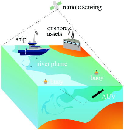
(a) Illustration of a range of ocean sensing opportunities.

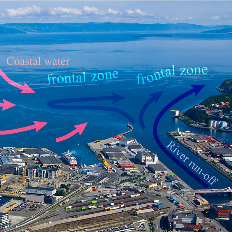
(b) Frontal patterns off of the Nidelva river, Trondheim, Norway.

Figure 1: 1(a) Traditional ocean observation based on ship-based sampling has been augmented by autonomous robotic vehicles such as AUVs. 1(b) The interaction of river and ocean creates processes that are challenging to map, where the combination of statistics and robotics can play a vital role in enabling more effective oceanographic observation.

Surveys with AUVs are usually limited to observations along fixed transects that are pre-scripted in mission plans created manually by a human operator. Missions can be specified operating on a scale of hundreds of meters to tens of kilometers depending on the scientific context. Faced with limited coverage capacity, a more effective approach is to instead use onboard algorithms to continuously evaluate, update, and refine future sampling locations, making the data collection adaptive. In doing so, the space of sampling opportunities is still limited by a waypoint graph, which forms a discretization of the search domain where the AUV can navigate; however the AUV can now modify its path at each waypoint based on in-situ measurements and calculations onboard using onboard deliberation (Py, Rajan and McGann, 2010; Rajan and Py, 2012; Rajan, Py and Berreiro, 2012). Full numerical ocean models based on complex differential equations cannot be run onboard the AUV with limited computational capacity, and statistical models relying on random field assumptions are relevant as a means to effectively update the onboard model from in-situ data, and to guide AUV data collection trajectories.

The work presented here is primarily inspired by a case study pertaining to using an AUV for spatial characterization of a frontal system generated by a river plume. Fig. 1(b) shows the survey area in Trondheim, Norway, where cold freshwater enters the fjord from a river, creating a strong gradient in both temperature and salinity. Because of the local topography and the Coriolis force the cold fresh water tends to flow east. Depending on the variations in river discharge, tidal effects, coastal current and wind, this boundary often gets distorted, and knowledge about its location is highly uncertain, making deterministic planning challenging. The goal is therefore to use AUV measurements for improved description of the interface between fresh and oceanic waters. It is often not possible to sample the biological variables of fundamental interest in such AUV operations, but off-the-shelf instruments provide temperature and salinity measurements which serve as proxys for the underlying biological phenomenon. With the help of a vector-valued random field model for temperature and salinity, one can then aim to describe the plume. The goal of plume characterization, in this way, relates to that of estimating some regions of the domain, typically excursion sets (ESs), when implicitly defined by the vector-valued random field. In our context of environmental sampling, the joint salinity and temperature excursions of a river plume help characterize the underlying bio-geochemical processes (Hopkins et al., 2013; Pinto et al., 2018). Motivating examples for ESs of multivariate processes are also abundant in other contexts, for instance in medicine, where physicians do not rely solely on a single symptom but must see several combined effects before making a diagnosis.

The questions tackled here hence pertain to the broader area of spatial data collection for vector-valued random fields. Given the operational constraints on AUV movements and the fact that surveys rely on successive measurements along a trajectory, addressing corresponding design problems calls for sequential strategies. Our main research angle in the present work is to extend sequential design strategies from the world of spatial statistics and computer experiments to the setting of both vector-valued observational data and experimental designs for feasible robotic trajectories. We leverage and extend recent progress in expected uncertainty reduction for ESs of Gaussian random fields (GRFs) in order to address this research problem. We briefly review recent advances in targeted sequential design of experiments based on GRFs before detailing other literature related to AUV sampling and our contributions prior to outlining the rest of the paper.

1.2 Random field modeling and targeted sequential design of experiments

While random field modeling has been one of the main topics throughout the history of spatial statistics (Krige, 1951; Stein, 1999), even for vector-valued random field models with associated prediction approaches such as co-Kriging (See, e.g., Wackernagel, 2003), there has lately been a renewed interest for random field models in the context of static or sequential experimental design, be it in the context of spatial data collection (Müller, 2007) or in simulation experiments (Santner, Williams and Notz, 2003). As detailed in Ginsbourger (2018), GRF models have been used in particular as a basis to sequential design of simulations dedicated to various goals such as global optimization and set estimation. Of particular relevance to our context, Bect et al. (2012) focuses on strategies to reduce uncertainties related to volumes of excursion exceeding a prescribed threshold, while Chevalier et al. (2014) concentrates on making the latter strategies computationally efficient and batch-sequential. Rather than focusing on excursion volumes, approaches were investigated in French and Sain (2013); Chevalier et al. (2013); Bolin and Lindgren (2015); Azzimonti et al. (2016) with ambitions of estimating sets themselves. Recently, sequential designs of experiments for the conservative estimation of ESs based on GRF models were presented in (Azzimonti et al., 2019).

Surprisingly less attention has been dedicated to sequential strategies in the case of vector-valued observations. It has been long acknowledged that co-Kriging could be updated efficiently in the context of sequential data assimilation (Vargas-Guzmán and Jim Yeh, 1999), but sequential strategies for estimating features of vector-valued random fields are still in their infancy. Le Gratiet, Cannamela and Iooss (2015) used co-Kriging based sequential designs to multi-fidelity computer codes and Poloczek, Wang and Frazier (2017) used related ideas for multi-information source optimization, but not for ES’s like we do here. More relevant to our setting, the PhD thesis (Stroh, 2018, p.82) mentions general possibilities of stepwise uncertainty reduction strategies for ES’s in the context of designing fire simulations, yet outputs are mainly assumed independent.

1.3 Previous work in AUV sampling

Other statistical work in the oceanographic domain include Wikle et al. (2013) focusing on hierarchical statistical models, Sahu and Challenor (2008) studying spatio-temporal models for sea surface temperature and salinity data and Mellucci et al. (2018) looking at the statistical prediction of features using an underwater glider. In this work the main focus is not on statistical modeling per se, but rather on statistical principles and computation underlying efficient data collection. We combine novel possibilities in marine robotics with spatial statistics and experimental design to provide useful AUV sampling designs.

Adaptive in-situ AUV sampling of an evolving frontal feature has been explored in Gottlieb et al. (2012); Smith et al. (2014); Pinto et al. (2018); Costa et al. (2018). These approaches typically use a reactive-adaptive scheme, whereby exploration does not rely on a statistical model of the environment, but rather adaptation is based on closing the sensing and actuation loop. Myopic sampling, i.e. stage-wise selection of the path (on the waypoint graph), has been used for surveys (Singh et al., 2009; Binney, Krause and Sukhatme, 2013) that focus largely on reducing predictive variance or entropy. These criteria are widely adopted in the statistics literature on spatio-temporal design as well (Bueso, Angulo and Alonso, 1998; Zidek and Zimmerman, 2019). However, response variance and entropy being depending only in GRF models on measurement locations and not on response values, criteria based on them only tend to have limited flexibility for active adaptation of trajectories based on measurement values. The use of data-driven adaptive criteria was introduced to include more targeted sampling of regions of scientific interest in Low, Dolan and Khosla (2009) and Fossum et al. (2018).

The primary contributions of this work are:

• Extending uncertainty reduction criteria to vector-valued cases.

• Closed-form expressions for the expected integrated Bernoulli variance (IBV) of the excursions in GRFs.

• Algorithms for myopic and multiple-step ahead sequential strategies for optimizing AUV sampling with respect to the mentioned criteria.

• Replicable experiments on synthetic cases with accompanying code

• Results from full-scale field trials running myopic strategies onboard an AUV for the characterization of a river plume.

The remainder of this paper is organized as follows: Section 2 defines ESs, excursion probabilities (EPs), and the design criteria connected to the IBV for excursions of vector-valued GRFs. Section 3 builds on these assumptions when deriving the sequential design criteria for adaptive sampling. In both sections properties of the methods are studied using simulations. Section 4 demonstrates the methodology used in field work characterizing a river plume. Section 5 contains a summary and a discussion of future work.

2 Quantifying uncertainty on Excursion Sets implicitly defined by GRFs

Section 2.1 introduces notation and co-Kriging equations of multivariate GRFs. Section 2.2 presents uncertainty quantification (UQ) techniques on ESs of GRFs, in particular the IBV and the excursion measure variance (EMV). Section 2.3 turns to the effect of new observations on EMV and IBV, and semi-analytical expected EMV and IBV over these observations are derived. Section 2.4 illustrates the concepts on a bivariate example relevant for temperature and salinity in our case.

2.1 Background, Notation and co-Kriging

We denote by $Z$ a vector-valued random field indexed by some arbitrary domain $\mathcal{M}$, and assume values of the field at any fixed location $u\in\mathcal{M}$, denoted $Z_{u}$, to be a $p$-variate random vector ($p\geq 2$). In the river plume characterization case, $\mathcal{M}$ is a prescribed domain in Trondheimsfjord, Norway (for the purpose of our AUV application, a discretization of a $2$-dimensional domain at fixed depth is considered), and $p=2$ with responses of temperature and salinity. A bivariate GRF model is assumed for $Z$. To motivate concepts, Fig. 2(a) and 2(b) shows a realization of such a vector-valued GRF on $\mathcal{M}=[0,1]^{2}$. Fig. 2(c) represents a by-product of interest derived from these realizations, namely regions: i) in red, where both temperature and salinity are high (i.e., exceeding respective thresholds), indicative of ocean water, ii) in white, where both temperature and salinity are low, indicative of riverine water, and iii) in light-red, where one variable is above and the other below their respective thresholds, indicative of mixed waters.

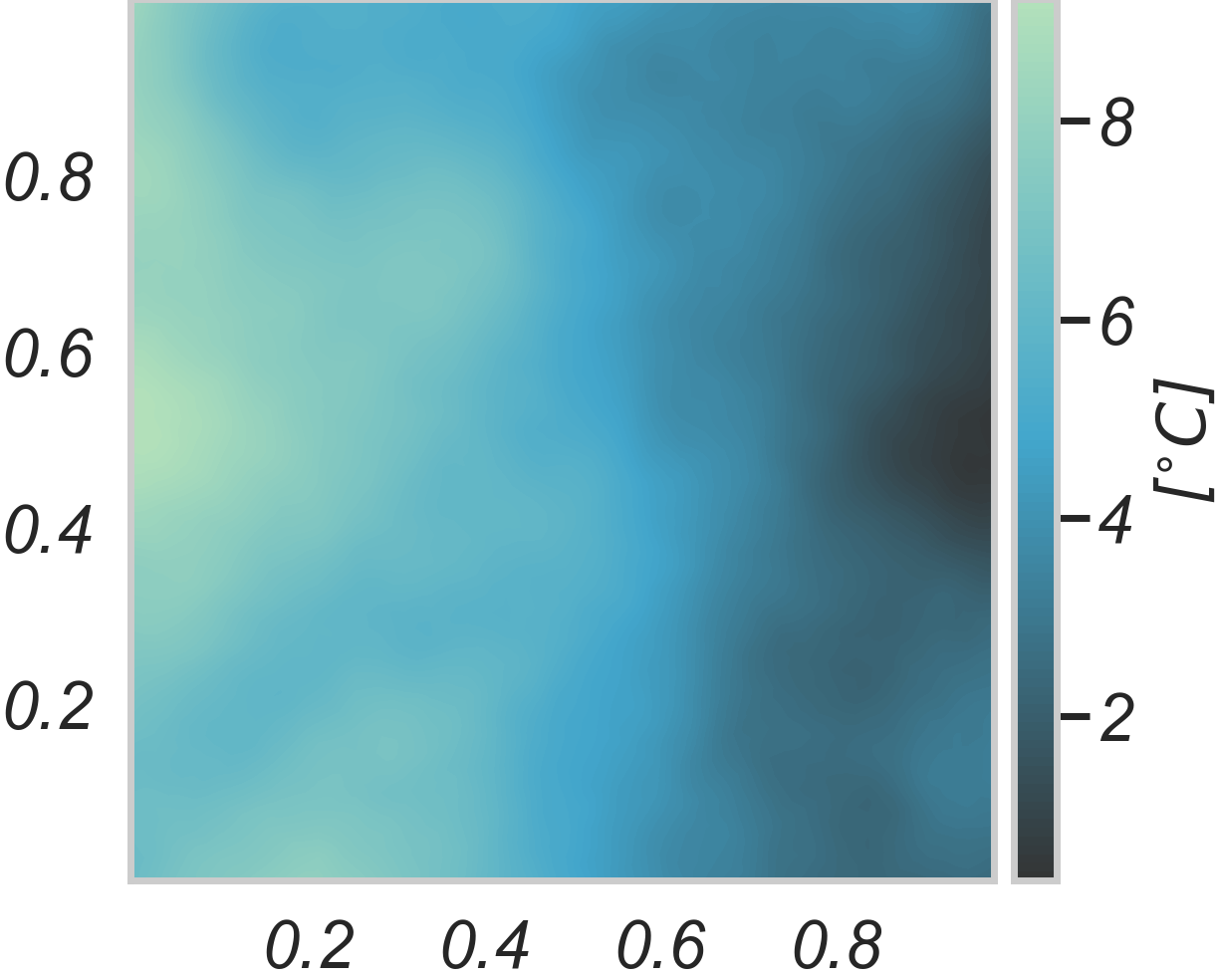
(a) Temperature.

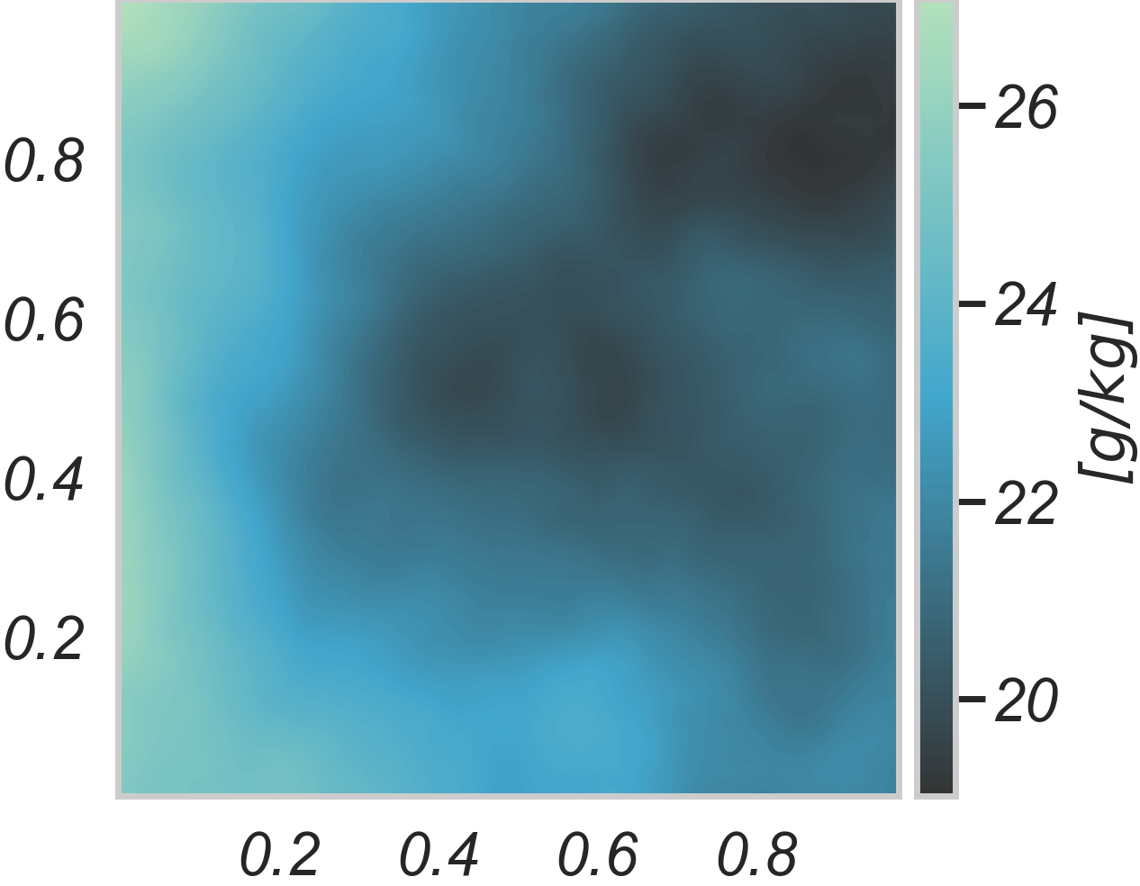
(b) Salinity.

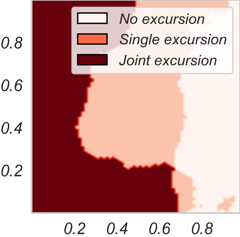
(c) Regions of interest.

Figure 2: Realization of a bivariate GRF (display (a) and (b)) and excursion set above some threshold (c). Joint excursion in red and excursion of a single variable in light-red.

For the general setting of a $p$-variate random field, we are interested in recovering the set of locations $\Gamma$ in the domain for which the components of $Z$ lie in some set of specified values $T\subset\mathbb{R}^{p}$; in other words the pre-image of $T$ by $Z$:

$$\Gamma:=Z^{-1}(T)=\{u\in\mathcal{M}:Z_{u}\in T\}.$$

If we assume that $Z$ has continuous trajectories and $T$ is closed, then $\Gamma$ becomes a Random Closed Set (Molchanov, 2005) and concepts from the theory of random sets will prove useful to study $\Gamma$. Note that while some aspects of the developed approaches do not call for a specific form of $T$, we will often, for purposes of simplicity, stay with the case of orthants ($T=(-\infty,t_{1}]\times\dots\times(-\infty,t_{p}]$ where $t_{1},\dots,t_{p}\in\mathbb{R}$) as this will allow efficient calculation of several key quantities. Note that changing some $\leq$ inequalities to $\geq$ ones would lead to immediate adaptations.

Letting $Z_{u,\ell}$ denote the $\ell\text{-th}$ component of $Z_{u}$ ($1\leq\ell\leq p$), we use the term generalized location for the couple $x=(u,\ell)$. The notation $Z_{x}$ will be used to denote $Z_{u,\ell}$ and will allow us to think of $Z$ as a scalar-valued random field indexed by $\mathcal{M}\times\{1\dots,p\}$, which will give the co-Kriging equations a particularly simple form that parallels the one of univariate Kriging. The letters $u$ and $\ell$ will be used for spatial locations and response indices respectively. Furthemore, boldface letters will be used to denote concatenated quantities corresponding to batches of observations. Given a dataset consisting of $q$ observations at spatial locations $\bm{u}=(u_{1},\dots,u_{q})\in\mathcal{M}^{q}$ and response indices $\bm{\ell}=(\ell_{1},\dots,\ell_{q})\in\{1,...,p\}^{q}$, we use the concatenated notation

$$\bm{x}:=(x_{1},\dots,x_{q}),~{}\text{with }x_{i}=(u_{i},\ell_{i}).$$

We also compactly denote the field values at those different locations by

$$Z_{\bm{x}}:=\left(Z_{u_{1},\ell_{1}},...,Z_{u_{q},\ell_{q}}\right)\in\mathbb{R}^{q}$$

For a second order random field $(Z_{u})_{u\in\mathcal{M}}$ with mean $\mu$ and matrix covariance function $K$, $\mu$ is naturally extended to $\mathcal{M}\in\{1,...,p\}$ into a function of $x=(u,\ell)$ and is further straightforwardly vectorized into a function of $\bm{x}$. As for $K$, it induces a covariance kernel $k$ on the set of extended locations via $k((u,\ell),(u^{\prime},\ell^{\prime}))=K(u,u^{\prime})_{\ell,\ell^{\prime}}$. In vectorized/batch form, $k(\bm{x},\bm{x}^{\prime})$ then amounts to a matrix with numbers of lines and columns equal to the numbers of generalized locations in $\bm{x}$ and $\bm{x}^{\prime}$, respectively. Such vectorized quantities turn out to be useful in order to arrive at simple expressions for the co-Kriging equations below.

Given a GRF $Z$ and observations of some of its components at locations in the domain, one can predict the value of the field at some unobserved location $u\in\mathcal{M}$ by using the conditional mean of $Z_{u}$, conditional on the data. This coincides with co-Kriging equations, which tell us precisely how to compute conditional means and covariances. We will present a general form of co-Kriging, in the sense that it allows inclusion of several (batch) observations at a time; observations at a given location $u\in\mathcal{M}$ may only include a subset of the components of $Z_{u}\in\mathbb{R}^{p}$ (heterotopic).

Assuming that $n$ batches of observations are available with sizes $q_{1},\dots,q_{n}$, and that one wishes to predict $Z_{\bm{x}}$ for some batch of $q\geq 1$ generalized locations $\bm{x}$, the simple co-Kriging mean then amounts to Kriging with respect to a scalar-valued GRF indexed by $\mathcal{M}\times\{1\dots,p\}$:

$$\mu_{[n]}(\bm{x})=\mu(\bm{x})+\lambda_{[n]}(\bm{x})^{T}(\mathbf{z}_{[n]}-\mu(\bm{x})).$$ (1)

Here, $\mathbf{z}_{[n]}$ stands for the ($\sum_{i=1}^{n}q_{i}$)-dimensional vector of observed (noisy) responses of $Z$ at all considered generalized locations, and $\lambda_{[n]}(\bm{x})$ is a vector of weights equal to

$$\left(k(\bm{x}_{[n]},\bm{x}_{[n]})+\Delta_{[n]}\right)^{-1}k(\bm{x}_{[n]},\bm{x})$$

with $\bm{x}_{[n]}=(\bm{x}_{1},\dots,\bm{x}_{n})$ and where $\Delta_{[n]}$ is the covariance matrix of Gaussian-distributed noise assumed to have affected measurements up to batch $n$. For our applications with salinity and temperature observations, this matrix is diagonal because we assume conditionally independent sensor readings, but it might not be diagonal with other types of combined measurements. The matrix in parenthesis will be assumed to be non-singular throughout the presentation. The associated co-Kriging residual (cross-)covariance function can also be expressed in the same vein via

$$k_{[n]}(\bm{x},\bm{x}^{\prime})=k(\bm{x},\bm{x}^{\prime})-\lambda_{[n]}(\bm{x})^{T}\left(k(\bm{x}_{[n]},\bm{x}_{[n]})+\Delta_{[n]}\right)\lambda_{{[n]}}(\bm{x}^{\prime}).$$ (2)

Let us now consider the case where a co-Kriging prediction of $Z$ was made with respect to $n$ batches of generalized locations, concatenated again within $\bm{x}_{[n]}=(\bm{x}_{1},\dots,\bm{x}_{n})$, and one wishes to update the prediction by incorporating a new vector of observations $\mathbf{z}_{n+1}$ measured at a batch of $q_{n+1}\geq 1$ generalized locations $\bm{x}_{n+1}$. Thanks to our representation of co-Kriging in terms of simple Kriging with respect to generalized locations, a strightforward adaptation of the batch-sequential Kriging update formulae from (Chevalier, Ginsbourger and Emery, 2013) suggests that

$$\mu_{[n+1]}(\bm{x})=\mu_{[n]}(\bm{x})+\lambda_{[n+1,n+1]}(\bm{x})^{T}(\mathbf{z}_{n+1}-\mu(\bm{x}_{n+1})),$$ (3)

where $\lambda_{[n+1,n+1]}(\bm{x})$ denotes the $q_{n+1}$-dimensional sub-vector extracted from $\lambda_{[n+1]}(\bm{x})$ that corresponds to the Kriging weights for the last $q_{n+1}$ responses when predicting at $\bm{x}$ relying on all measurements until batch $(n+1)$. The associated co-Kriging residual (cross-)covariance function is

$$k_{[n+1]}(\bm{x},\bm{x}^{\prime}) =k_{[n]}(\bm{x},\bm{x}^{\prime})$$ (4)

$$- \lambda_{[n+1,n+1]}(\bm{x})^{T}\left(k_{[n]}(\bm{x}_{n+1},\bm{x}_{n+1})+\Delta_{n+1}\right)\lambda_{{[n+1,n+1]}}(\bm{x}^{\prime}),$$

As noted in (Chevalier, Emery and Ginsbourger, 2015) in the case of scalar-valued fields, these update formulae naturally extend to universal Kriging in second-order settings and apply without Gaussian assumptions. We will now see how the latter formulae are instrumental in deriving semi-analytical formulae for step-wise uncertainty reduction criteria for vector-valued random fields.

2.2 Uncertainty Quantification on ESs of multivariate GRFs

We now introduce quantities that allow UQ on the volume of the ES $\Gamma$. Let $\nu$ be a (locally finite, Borel) measure on $\mathcal{M}$. We want to investigate the probability distribution of $\nu(\Gamma)$ through its moments. Centered moments may be computed using Proposition 3 developed in the appendix. In particular, as an integral over EPs, the $\operatorname{EMV}=\operatorname{Var}[\nu(\Gamma)]$ is:

$$\begin{split}\operatorname{EMV}&=\int_{\mathcal{M}^{2}}\mathbb{P}\left(Z_{u}\in T,Z_{v}\in T\right)d\nu^{\otimes}(u,v)\\ &-\left(\int_{\mathcal{M}}\mathbb{P}\left(Z_{u}\in T\right)d\nu(u)\right)^{2},\end{split}$$

which in the excursion/sojourn case where $T=(-\infty,t_{1}]\times\dots\times(-\infty,t_{p}]$ is

$$\begin{split}\operatorname{EMV}&=\int_{\mathcal{M}^{2}}\varPhi_{2p}\left(({\bm{t}},{\bm{t}});\mu((u,v)),K((u,v),(u,v))\right)\ \mathrm{d}\nu^{\otimes}(u,v)\\ &-\left(\int_{\mathcal{M}}\varPhi_{p}\left({\bm{t}};\mu(u),K(u)\right)d\nu(u)\right)^{2},\end{split}$$

where $\varPhi_{p}$ denotes the $p$-variate Gaussian cumulative distribution function (CDF) numerically (Genz and Bretz, 2009).

Note that this quantity requires the solution of an integral over $\mathcal{M}^{2}$. In contrast, the IBV of Bect, Bachoc and Ginsbourger (2019) involves solely an integral on $\mathcal{M}$ and can be expanded as

$$\begin{split}\operatorname{IBV}&=\int_{\mathcal{M}}\mathbb{P}\left(Z_{u}\in T\right)(1-\mathbb{P}\left(Z_{u}\in T\right))d\nu(u)\\ &=\int_{\mathcal{M}}\varPhi_{p}\left({\bm{t}};\mu(u),K(u)\right)-\left(\varPhi_{p}\left({\bm{t}};\mu(u),K(u)\right)\right)^{2}\mathrm{d}\nu(u).\end{split}$$

2.3 Expected IBV and EMV

We compute the expected effect of the inclusion of new observations on the $\operatorname{EMV}$ and $\operatorname{IBV}$ of the ES $\Gamma$. Let us consider the same setting as in Eq. (3) and (4), and let $\mathbb{E}_{[n]}\left[.\right]$ and $\mathbb{P}_{[n]}\left(.\right)$ denote conditional expectation and probability conditional on the first $n$ batches of observations, respectively. We use $\operatorname{IBV}_{n}$ to denote $\operatorname{IBV}$ with respect to the conditional law $\mathbb{P}_{n}$.

In order to study the effect of the inclusion of a new data point, we let $\operatorname{IBV}_{[n]}(\bm{x};\bm{y})$ denote the expected IBV under the current law of the field, conditioned on observing $\bm{y}$ at $\bm{x}$ (generalized, possibly batch observation). The expected effect of a new observation on the IBV is then

$$\operatorname{EIBV}_{[n]}(\bm{x}):=\mathbb{E}_{[n]}\left[\mbox{IBV}(\bm{x};\bm{Y})\right],$$ (5)

where $\bm{Y}$ is distributed according to the current law of $Z_{\bm{x}}$ and with independent noise having covariance matrix $\Delta_{n}$.

We next present a result that allows efficient computation of $\operatorname{EIBV}$ as an integral of CDFs of the multivariate Gaussian distribution. This will prove useful when designing sequential expected uncertainty reduction strategies.

Proposition 1.

$$\begin{split}\operatorname{EIBV}_{[n]}(\bm{x})&=\int_{\mathcal{M}}\varPhi_{p}\left({\bm{t}};~{}\mu_{[n]}\left(u\right),K_{[n]}\left(u,u\right)\right)d\nu(u)\\ &-\int_{\mathcal{M}}\varPhi_{2p}\left(\left(\begin{matrix}{\bm{t}}-\mu_{[n]}\left(u\right)\\ {\bm{t}}-\mu_{[n]}\left(u\right)\end{matrix}\right);\mathbf{\Sigma}_{[n]}(u)\right)d\nu(u),\end{split}$$ (6)

where the matrix $\mathbf{\Sigma}_{[n]}(u)$ is defined as

$$\begin{split}\mathbf{\Sigma}_{[n]}(u)&=\left(\begin{matrix}K_{[n]}\left(u,u\right)&K_{[n]}\left(u,u\right)-K_{[n+1]}\left(u,u\right)\\ K_{[n]}\left(u,u\right)-K_{[n+1]}\left(u,u\right)&K_{[n]}\left(u,u\right)\end{matrix}\right).\\ \end{split}$$

As for the expected EMV, a similar result may be derived.

Proposition 2.

$$\begin{split}\operatorname{EEMV}_{[n]}(\bm{x})&=\int_{\mathcal{M}^{2}}\varPhi_{2p}\left(({\bm{t}},{\bm{t}});~{}\mu((u,v)),K((u,v),(u,v))\right)\ \mathrm{d}\nu^{\otimes}(u,v)\\ &-\int_{\mathcal{M}^{2}}\varPhi_{2p}\left(\left(\begin{matrix}{\bm{t}}-\mu_{[n]}\left(u\right)\\ {\bm{t}}-\mu_{[n]}\left(v\right)\end{matrix}\right);~{}\mathbf{\tilde{\Sigma}}_{[n]}(u,v)\right)\mathrm{d}\nu^{\otimes}(u,v)\end{split}$$

where the matrix $\mathbf{\tilde{\Sigma}}_{[n]}(u,v)$ is defined blockwise as

$$\begin{split}\mathbf{\tilde{\Sigma}}_{[n]}(u,v)&=\left(\begin{matrix}\tilde{\Sigma}_{1,1}(u,u)&\tilde{\Sigma}_{1,2}(u,v)\\ \tilde{\Sigma}_{2,1}(v,u)&\tilde{\Sigma}_{2,2}(v,v)\end{matrix}\right)\end{split}$$

with blocks given, for $i,j\in\{1,2\}$ and $u,v\in\mathcal{M}$, by

$$\begin{split}\tilde{\Sigma}_{i,j}(u,v)&=\lambda_{[n+1,n+1]}(u)^{T}k_{[n]}(\bm{x},\bm{x})\lambda_{[n+1,n+1]}(v)+\delta_{i,j}K_{[n+1]}\left(u,v\right).\end{split}$$

We remark that Propositions 1 and 2 are twofold generalizations of results from Chevalier et al. (2014): they extend previous results to the multivariate setting and also allow for the inclusion of batch or heterotopic observations through the concept of generalized locations. A key element for understanding these propositions is that the conditional co-Kriging mean entering in the EPs depend linearly on (batch) observations. The conditional equality expressions thus become linear combinations of Gaussian variables whose mean and covariance are easily calculated. Related closed-form solutions have been noted in similar contexts (Bhattacharjya, Eidsvik and Mukerji, 2013; Stroh, 2018), but not generalized to our situation with random sets for vector-valued GRFs.

2.4 Expected Bernoulli variance for a two dimensional Example

We illustrate the expected Bernoulli variance (EBV) associated with different designs on a bivariate example. This mimics our river plume application and hence the first and second component of the random field will be called temperature and salinity. We begin with a pointwise example, considering a single bivariate Gaussian distribution (i.e. no spatial elements).

2.4.1 A pointwise study

Say we want to study the excursion probability of a bivariate Gaussian above some threshold, where the thresholds are set equal to the mean; $\mu_{1}=t_{1}=5^{o}C$ for temperature and $\mu_{2}=t_{2}=30$ g/kg for salinity, and we play with the temperature and salinity correlation and variances to study the effect on the EP and EBV.

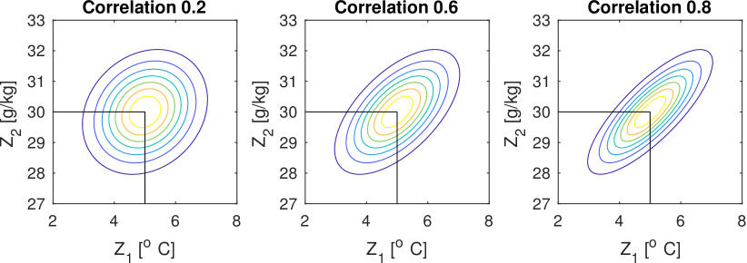
Figure 3: Density contour plots with increasing correlations between temperature and salinity. The densities have unit variance and thresholds identical to the mean values $5^{o}C$ and $30$ g/kg.

Fig. 3 shows contour plots of three different densities with increasing correlation $\gamma$ between temperature and salinity. The displayed densities have unit standard deviations for both temperature and salinity, but we also study the effect of doubling the standard deviations.

Table 1 shows the initial EPs and the associated Bernoulli variance (second row) for the examples indicated in Fig. 3. The EPs increase with the correlation as there is a strong tendency to have jointly low or high temperature and salinity. The Bernoulli variance is similarly larger for high correlations. EPs and Bernoulli variances are the same for temperature and salinity standard deviations $\sigma_{1}$ and $\sigma_{2}$, which implies that high variability in temperature and salinity is not captured in the $p(1-p)$ expression.

Table 1: EP and Bernoulli variance for different correlations and variances (top rows), and EBVs for both temperature and salinity data, and only temperature data (bottom rows).

	$\sigma_{1}=\sigma_{2}=1$			$\sigma_{1}=\sigma_{2}=2$
Correlation $\gamma$	0.2	0.6	0.8	0.2	0.6	0.8
$p$	0.28	0.35	0.40	0.28	0.35	0.40
$p(1-p)$	0.20	0.23	0.24	0.20	0.23	0.24
EBV, Temperature and Salinity	0.092	0.089	0.085	0.052	0.051	0.049
EBV, Temperature only	0.151	0.138	0.123	0.137	0.114	0.093

The bottom two rows of Table 1 show EBV results. This is presented for a design gathering both data types, and for a design with temperature measurements alone. When both data are gathered, the measurement model is $(Y_{1},Y_{2})^{t}=(Z_{1},Z_{2})^{t}+{\bm{\epsilon}}$, with ${\bm{\epsilon}}\sim N(0,0.5^{2}I_{2})$, while $Y_{1}=Z_{1}+\epsilon$, $\epsilon\sim N(0,0.5^{2})$ when only temperature is measured. For this illustration, Table 1 shows that the expected Bernoulli variance gets smaller with larger standard deviations. The expected reduction of Bernoulli variance is further largest for the cases with high correlation $\gamma$. Albeit smaller, there is also uncertainty reduction when only temperature is measured (bottom row), especially when temperature and salinity are highly correlated. When correlation is low ($\gamma=0.2$), there is little information about salinity in the temperature data, and therefore less uncertainty reduction.

2.4.2 Including Spatiality

We now turn to an example involving a full-fledged GRF. The statistical model we consider has a linear trend

$$\mu(s)=\mathbb{E}\left[\begin{pmatrix}Z_{u,1}\\ Z_{u,2}\end{pmatrix}\right] =\beta_{0}+\beta_{1}u,$$

with $\beta_{0}$ a two dimensional vector and $\beta_{1}$ a $2\times 2$ matrix. In our examples, we only consider separable covariance models;

$$\textrm{Cov}\left(Z_{u,i},Z_{v,j}\right) =k(u,v)\gamma(i,j),~{}\gamma(i,j)=\begin{cases}\sigma_{i}^{2},~{}i=j\\ \gamma\sigma_{i}\sigma_{j},~{}i\neq j,\end{cases}$$

where an isotropic Matérn 3/2 kernel $(1+\eta h)\exp(-\eta h)$ is used, for Euclidean distance $h$. In the accompanying Python examples taking place within the MESLAS toolbox , these modeling assumptions can however be relaxed to anisotropic covariance and changing variance levels across the spatial domain. Both extensions are relevant for the setting with river plumes, but in practice this requires more parameters to be specified. With extensive satellite data or prior knowledge from high-resolution ocean models, one could also possibly fit more complex multivariate spatial covariance functions (Gneiting, Kleiber and Schlather, 2010; Genton and Kleiber, 2015), but that is outside the scope of the current work.

In the rest of this section, we consider a GRF with mean and covariance structure as above and parameters

$$\beta_{0}=\begin{pmatrix}5.8\\ 24.0\end{pmatrix},~{}\beta_{1}=\begin{pmatrix}0.0&-4.0\\ 0.0&-3.8\end{pmatrix},~{}\sigma_{1}=2.5,~{}\sigma_{2}=2.25,~{}\gamma=0.2,$$

and kernel parameter $\eta=3.5$. One realization of this GRF is shown in Fig. 2. In the computed examples, the spatial domain $\mathcal{M}$ is discretized to a set of $N$ grid locations $\mathcal{M}_{g}=\{u_{i},i=1,\ldots,N\}$, where each cell has area $\delta$; the same grid is used for the waypoint graph for possible design locations. The EIBV is approximated by sums over all grid cells.

We now study how the EBV [Eq.(5)] associated with data collection at a point changes if only one of the two components of the field is observed. We first draw a realization of the GRF defined above and use it as ground-truth to mimic the real data-collection process. A first set of observations are done at the locations depicted in grey (see Fig. 4), and the data is used to update the GRF model. We then consider the green triangle as a potential next observation location and plot the EBV reduction (at each grid node in the waypoint graph) that would result from observing only one component of the field (temperature or salinity), or both at that point.

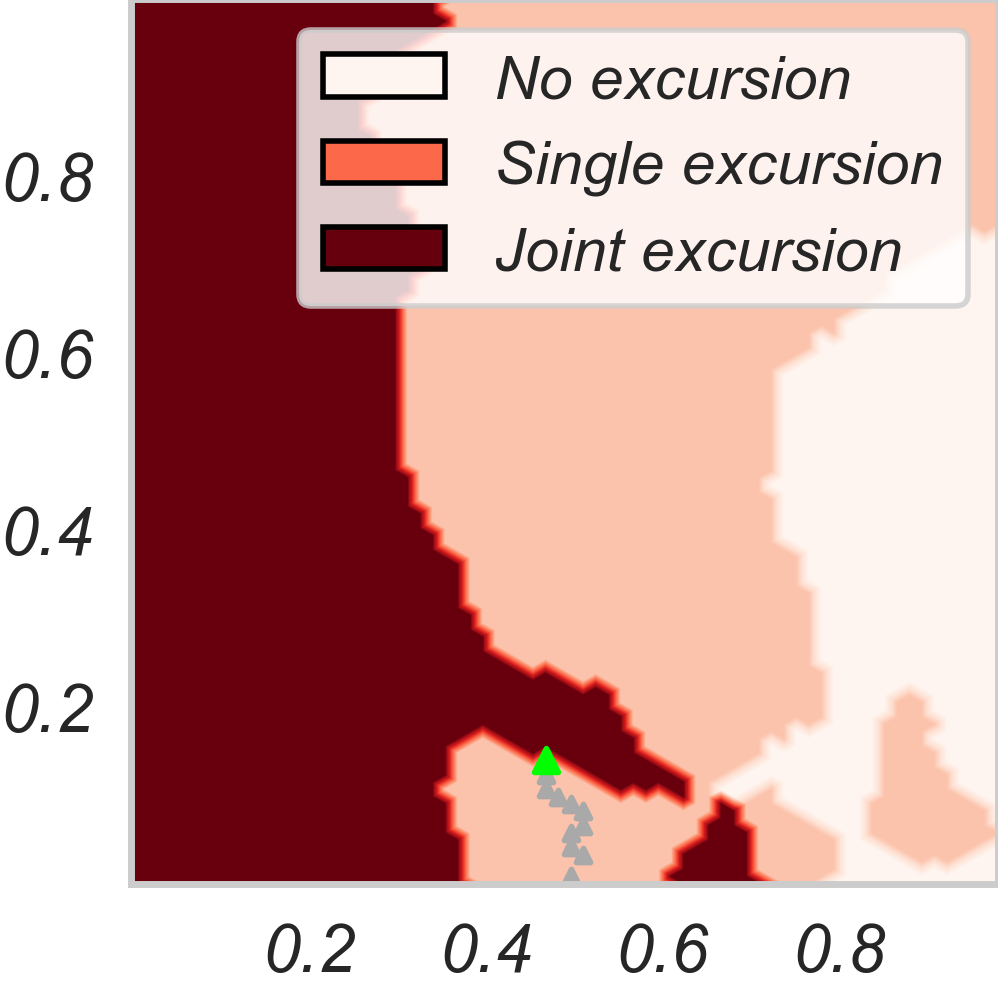
(a) Regions of interest.

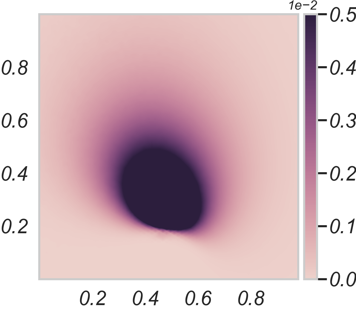
(b) Temperature.

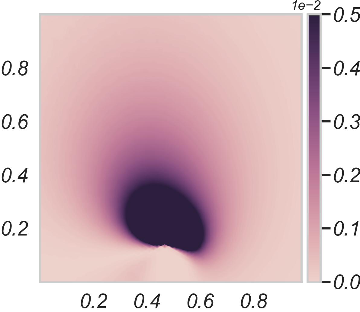
(c) Salinity.

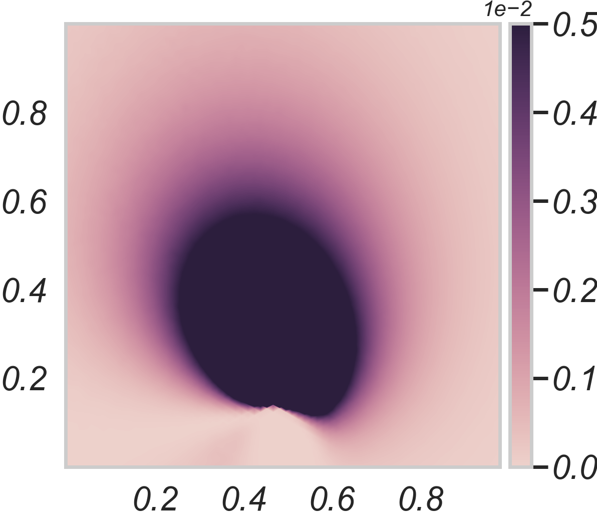
(d) Both.

Figure 4: Pointwise Bernoulli variance reduction for observation of a single or both components of the random field at one location. Data collection locations in green. True excursion set in red. Places where only one response is above threshold are depicted in pink. EBV reduction associated to observing one or both responses at the green location are shown in 4(b), 4(c) and 4(d).

Note that plotting the EBV reduction at each point might also be used to compare different data collection plans. For example, Fig. 5 shows the EBV reduction associated with a data collection plan along a vertical line (static north) and one associated with a horizontal (static east). Both expectations are computed according to the a-priori distribution of the GRF (i.e. no observations have been included yet).

(a) Excursion probability.

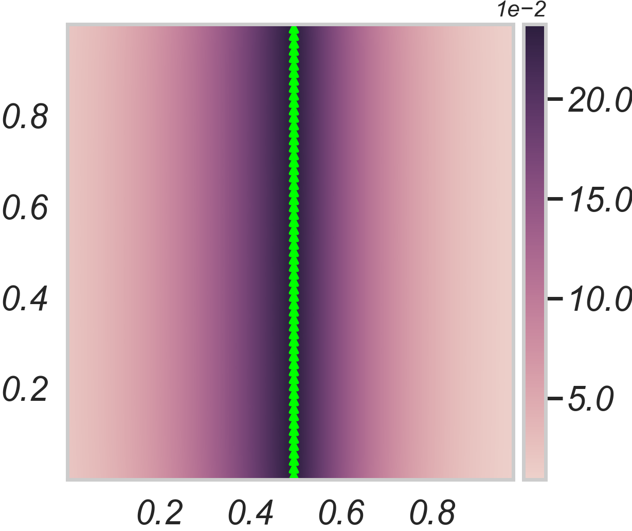
(b) Static north design.

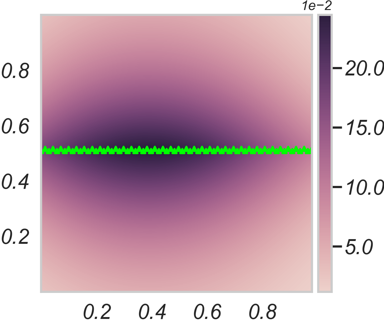
(c) Static east design.

Figure 5: Pointwise Bernoulli variance reduction for two different static designs (later noted as static_north and static_east). The prior EP is shown in 5(a). EBV reduction for each design shown in 5(b) and 5(c).

3 Sequential designs and heuristic path planning

We present sequential data collection strategies that aim at reducing the expected uncertainty on the target ES $\Gamma$.

3.1 Background

From a sequential point of view, $n$ data collection steps have already been performed and one wants to choose what data to collect next. The design evaluations are based on the conditional expectation $\mathbb{E}_{[n]}\left[.\right]$ from the law of the field, conditional on all data available at stage $n$. Once the best design at stage $n$ has been selected, the data are collected and the GRF model is updated using co-Kriging Eq. 3 and 4, yielding a conditional law $\mathbb{P}_{n+1}$ after which the process is repeated.

Note that the type of data collected at each stage can be of various type (all components of the field at a single location, only some components at a subset of selected locations, etc.) because of the concept of generalized location in the co-Kriging expressions. In general, a design strategy must choose the spatial location as well as the components to observe (heterotopic), or where several observations are allowed at each stage (batch). For the case with an AUV exploring the river plume, we limit our scope to choosing one of the neighboring spatial location (waypoints) at each stage, and all components (temperature and salinity) of the field are observed (isotopic). The candidate points at this stage are denoted $\mathcal{J}$ as defined from the 6 directions (apart from edges) in the waypoint graph (see Fig. 7(a)). The set $\mathcal{J}$ depends on the current location, but for readability we suppress this in the notation.

The mathematical expression for the optimal design in this sequential setting involves a series of intermixed maximizations over designs and integrals over data. In practice, the optimal solution is intractable because of the enormous growth over stages (see e.g. Powell (2016)). Instead, we outline heuristic strategies.

3.2 A Naive Sampling Strategy

A simple heuristic for adaptive sampling is to observe $Z$ at the location in $\mathcal{J}$ with current EP closest to $\frac{1}{2}$. While easy to implement, this strategy can lead to spending many stages in boundary regions regardless of the possible effect of sampling at the considered point for the future conditional distribution of $Z$. The strategy does not account for the expected reduction in uncertainty, and it does not consider having an integrated effect over other locations.

3.3 Myopic Path Planning

The myopic (greedy) strategy which we present here is optimal if we imagine taking only one more stage of measurements; it does not anticipate what the subsequent designs might offer beyond the first stage. Based on the currently available data the myopic strategy selects the location that leads to the biggest reduction in EIBV:

Criterion (Myopic).

The next observation location $u_{n+1}$ is chosen among the minimizers in $\mathcal{J}$ of the criterion:

$$C_{\text{myopic}}(u)=\operatorname{EIBV}_{n}\left(u\right)$$ (7)

The EIBV is efficiently computed for each of the candidate points $\mathcal{J}$ using Proposition 4. Even though this myopic strategy is non-anticipatory, it still provides a reasonable approach for creating designs in many applications. Moreover, it can be implemented without too much demand on computational power, making it well-suited for embedding on an AUV.

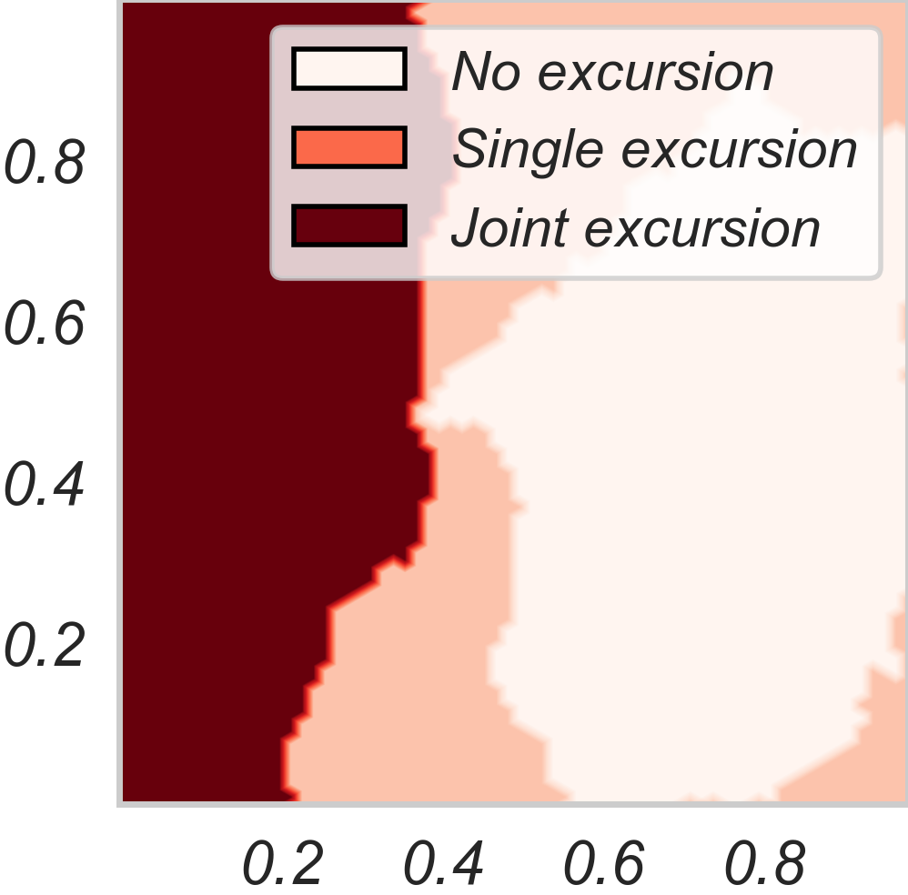
(a) Excursion realization.

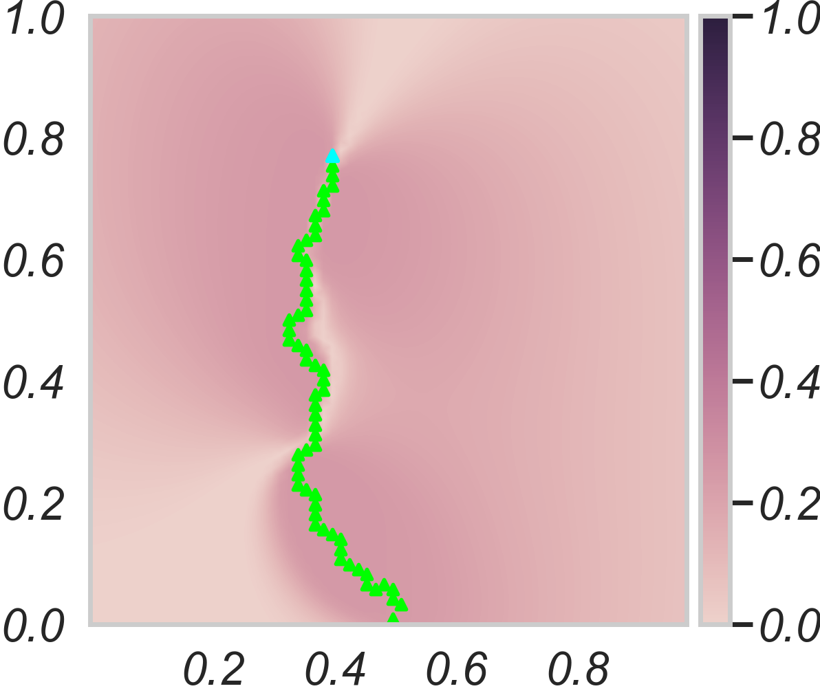
(b) BV reduction.

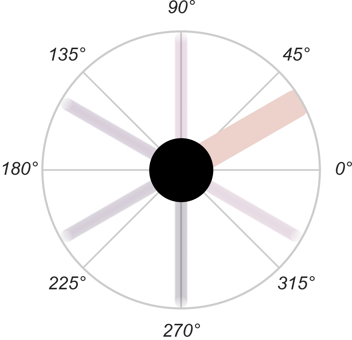
(c) Expected reduction of BV.

Figure 6: Example run of the myopic strategy on a realisation of the GRF model from 2.4.2. Reduction in Bernoulli variance compared to the prior is shown in 6(b), with past observation locations in green and current AUV position in cyan. The expected IBV reduction associated to data collection at neighbouring nodes of the current location is shown in 6(c). The thick and light color indicates the node at $30^{\circ}$ to be the best possible choice.

3.4 Look-ahead Trajectory Planning

We now extend the myopic strategy by considering two stages of measurements, which is optimal in that it accounts consistently for the expectations and minimizations in these two stages, but no anticipation beyond that.

The principle of two-step look-ahead is to select the next observation location $u_{n+1}$ that yields the biggest reduction in EIBV if we were to (optimally) add one more observation after that again. In order to formalize this concept, we must extend the notation for EIBV in the future (after observation $n+1$ has been made). We let $\operatorname{EIBV}_{[n]}(\cdot;u,y)$ denote the EIBV where expectations are taken conditional on the data available at stage $n$ and on an additional observation $y$ at $u$ at stage $n+1$.

Criterion (2-step look-ahead).

The next observation location $u_{n+1}$ is chosen among the minimizers in $\mathcal{J}$ of the criterion

$$C_{\text{2-steps}}(u) =\mathbb{E}_{n}\left[\min_{u^{\prime}\in\mathcal{J}(u)}\operatorname{EIBV}_{n}\left(u^{\prime};u,Y\right)\right]$$ (8)

where $Y$ is the random data realization of $Z_{u}$ according to its conditional law at step $n$ with the dependence of the set of candidates on the current location having been made explicit for the second stage of measurements.

In a practical setting, the first expectation can be computed by Monte Carlo sampling of data $Y$ from its conditional distribution. For each of these data samples, the second expectation is solved using the closed-form expressions for EIBV provided by Proposition 4, now with conditioning on the first stage data already going into the co-Kriging updating equations.

3.5 Simulation studies

3.5.1 Static and Sequential Sampling Designs

We compare three different static designs denoted static_north, static_east, and static_zigzag (a version of static_north where with some east-west transitions in a zigzag pattern) with the three described sequential approaches naive, myopic, and look-ahead. The static AUV sampling paths are pre-scripted and cannot be altered. For a fixed survey length, a closed-form expression for the EIBV is available as in Proposition 1. However, for the sequential approaches this is not the case. For comparison, the properties are therefore evaluated using Monte Carlo integration over several replicates of realizations from the model while conducting simulated sequential surveys for each one. An example of such a realization with a myopic strategy is shown in Fig. 6.

We also compare predictive performance measured by root mean square error (RMSE) for temperature and salinity estimates as well as the variance reduction in these two variables. It is important to note that the objective function used by the AUV is focused on reducing the EIBV, but we nevertheless expect that we will achieve good predictive performance for criteria such as RMSE as well. Another non-statistical criterion that is important for practical purposes is the computational time needed for the strategy.

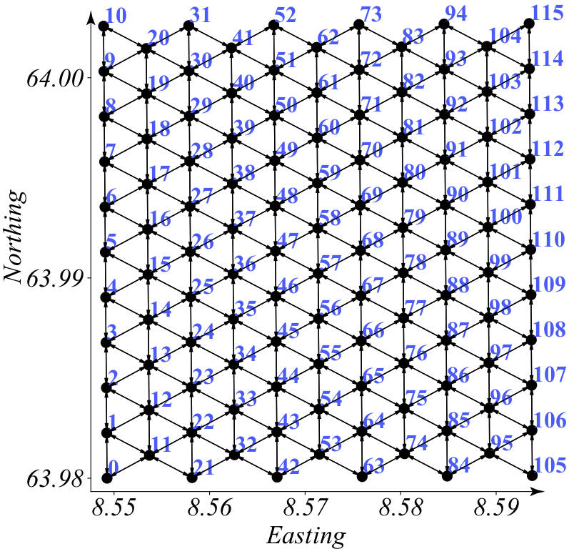
(a) The waypoint graph.

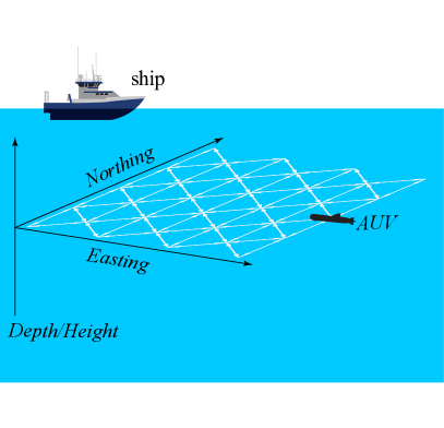
(b) The waypoint graph in 3D.

Figure 7: 7(a) The equilateral waypoint graph used to discretize the trajectory choices over the $31\times 31$ grid used to discretize the GRF. The AUV is set to start in node $53$. 7(b) The waypoint grid shown in a 3D environment.

Each strategy is conducted on an equilateral grid as shown in Fig. 7. The AUV starts at the center coordinate at the southern end of the domain (node 53). It then moves along edges in the waypoint graph while collecting data which are assimilated onboard to update the GRF model. This is used in the evaluation of the next node to sample. The procedure is run for $10$ stages. A total of 100 replicate simulations were conducted with all strategies.

3.5.2 Simulation Results

The results of the replicate runs are shown in Fig. 8, where the different criteria are plotted as a function of survey distance. Fig. 8(a) shows the resulting drop in realized IBV for each of the six strategies. IBV reduction is largest for the myopic and look-ahead strategies, each performing almost equally; this is expected as the two criteria (Eq. (7) and (8)) are sensitive to differences in IBV. The static_north design also does well here because the path is parallel to the boundary between the water masses.

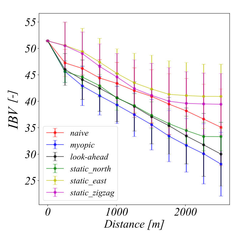
(a) IBV.

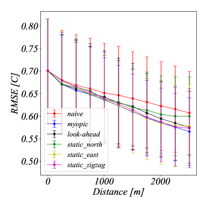
(b) RMSE between estimated field and truth.

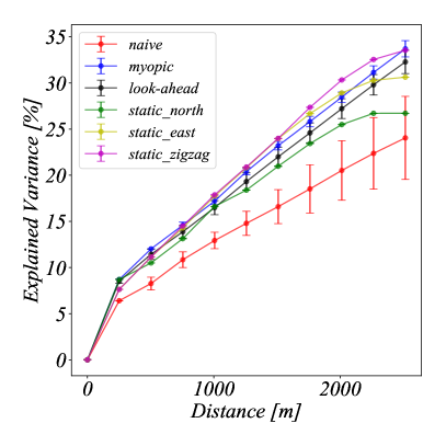
(c) Explained variance ${\bm{R}}^{2}$.

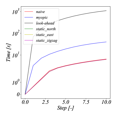
(d) Computational time for inference (the lines for naive, static_north, static_east, and static_zigzag overlap).

Figure 8: Simulation results from 100 replicate simulations for 10 sampling choices/stages on the grid. Vertical lines show variation in replicate results.

Fig. 8(b) and 8(c) show the resulting drop in RMSE and increase in explained variance, respectively. Both myopic and look-ahead strategies perform well here, but some of the static_east and static_zigzag also achieve good results because they cover large parts of the domain without re-visitation. Sequential strategies targeting IBV will sometimes not reach similar coverage, as interesting data may draw the AUV into twists and turns. There is a relatively large variety in the replicate results as indicated by the vertical lines. Nevertheless, the ordering of strategies is similar.

Fig. 8(d) shows the computational effort: the naive strategy is on par with the static designs, while the myopic strategy is slower because it evaluates expected values for all candidate directions at the waypoints. But it is still able to do so in reasonable time, which allows for real-world applicability. The look-ahead strategy is much slower, reaching levels that are nearly impractical for execution on an AUV. Some pruning of the graph is performed to improve the performance, such as ruling out repeated visitations. Further pruning of branches or inclusion of other heuristics could be included for better performance. Then again, the inclusion of such heuristics is likely a contributing factor for the look-ahead strategy failing to outperform the myopic strategy.

We studied the sensitivity of the results by modifying the input parameters to have different correlations between temperature and salinity, standard deviations, and spatial correlation range. In all runs, the myopic and look-ahead strategies perform the best in terms of realized IBV, and much better than naive. The look-ahead strategy seems to be substantially better than the myopic design only for very small initial standard deviations or very large spatial correlation range. We also ran simulation studies with only temperature data, and for realistic correlation levels between temperature and salinity, the IBV results are not much worse when only temperature data are available. In addition to the comparison made in Table 1, the current setting includes spatial correlation and this likely strengthen the effect of temperature information. However, it seems that having temperature data alone does a substantially worse job in terms of explained variance.

4 Case Study - Mapping a River Plume

To demonstrate the applicability of using multivariate EPs and the IBV to inform oceanographic sampling, we present a case study mapping a river plume with an AUV. The experiment was performed in Trondheim, Norway, surveying the Nidelva river (Fig. 1(b)). The experiments were conducted in late Spring 2019, when there is still snow melting in the surrounding mountains so that the river water is colder than the water in the fjord. The experiment was focused along the frontal zone that runs more or less parallel to the eastern shore.

4.1 Model Specification

The statistical model parameters were specified based on a short preliminary survey where the AUV made an initial transect to determine the trends in environmental conditions and correlation structures. Based on the initial runs we get a reasonable idea of the temperature and salinity of river and ocean waters, and also specify the trend by linear regression, where both temperature and salinity were assumed to increase linearly with the west coordinate. Next, the residuals from the regression analysis were analyzed to specify the covariance parameters of the GRF model.

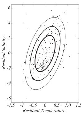
(a) Residual plot.

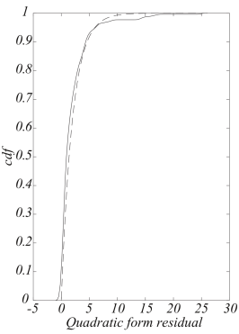
(b) Empirical CDF.

(c) Empirical variogram.

Figure 9: Data analysis from a preliminary trial experiment using the AUV. 9(a) Residual plot of temperature and salinity along with Gaussian contours. 9(b) Empirical CDF (solid) of the quadratic form of the residuals along with the theoretical CDF (dashed) of the $\chi^{2}$ distribution with two degrees of freedom. 9(c) Empirical variogram of the salinity and temperature data.

Fig. 9 summarizes diagnostic plots of this analysis. Fig. 9(a) shows a cross-plot of temperature and salinity residuals after the regression mean values of salinity and temperature are subtracted from the data. This scatter-plot of joint residuals indicates larger variability in salinity than temperature, and a positive correlation ($0.5$) between the two variables. Based on the fitted bivariate covariance model (ellipses in Fig. 9(a)), we can compute the scalar quadratic form of the residuals, and if the model is adequate they should be approximately $\chi^{2}_{2}$ distributed. Fig. 9(b) shows the empirical CDF of the quadratic forms (solid) together with the theoretical CDF of the $\chi^{2}_{2}$ distribution (dashed). The modeled and theoretical curves are rather similar, which indicates that the Gaussian model with constant spatial variance and correlation fits reasonably well. Fig. 9(c) shows the empirical variogram of the residuals for temperature and salinity. The decay is similar for the two, and seems to be negligible after about $150$ m. The working assumption of a separable covariance function is hence not unreasonable.

Based on the analysis in Fig. 9, the resulting parameters are given in Table 2. The regression parameters shown here are scaled to represent the east and west boundaries of the domain as seen in the preliminary transect data, and the thresholds are intermediate values. These parameter values were then used in field trials where we explored the algorithm’s ability to characterize the river plume front separating the river and fjord water masses.

Parameter	Value	Source
Cross correlation temperature and salinity	0.5	AUV observations
Temperature variance	0.20	AUV observations (variogram)
Salinity variance	5.76	AUV observations (variogram)
Correlation range	0.15 km	AUV observations (variogram)
River temperature	$10.0\,^{\circ}\mathrm{C}$	AUV observations
Ocean temperature $T_{ocean}$	$11.0\,^{\circ}\mathrm{C}$	AUV observations
River salinity $S_{river}$	$14.0$ g/kg	AUV observations
Ocean salinity $S_{ocean}$	$22.0$ g/kg	AUV observations
Threshold in temperature	$10.5\,^{\circ}\mathrm{C}$	User specified
Threshold in salinity	$18.0$ g/kg	User specified

Table 2: Model and threshold parameters from an initial AUV survey. Observations were taken across the front while crossing from fresh, cold river water to saline and warmer ocean waters.

4.2 Experimental Setup

A Light AUV (Sousa et al., 2012) (Fig. 10) equipped with a 16 Hz Seabird Fastcat-49 conductivity, temperature, and depth (CTD) sensor was used to provide salinity and temperature measurements. The AUV is a powered untethered platform that operates at $1$-$3$ m/s in the upper water column. It has a multicore GPU NVIDIA Jetson TX1 (quad-core 1.91 GHz 64-bit ARM machine, a 2-MB L2 shared cache, and 4 GB of 1600 MHz DRAM) for computation onboard. The sampling algorithm was built on top of the autonomous Teleo-Reactive EXecutive (T-REX) framework (Py, Rajan and McGann, 2010; Rajan and Py, 2012; Rajan, Py and Berreiro, 2012). We assume that the measurements are conditionally independent because the salinity is extracted from the conductivity sensor which is different from the temperature sensor. We specify variance $0.25^{2}$ for both errors, which is based on a middle ground between the nugget effect in the empirical variogram and the sensor specifications.

Figure 10: The commercially available Light Autonomous Underwater Vehicle (LAUV) platform for upper water-column exploration used in our experiments.

The AUV was running a myopic strategy to decide between sampling locations on the waypoint graph distributed over an equilateral grid, as shown in the grey-colored lattice in Fig. 11(a). At each stage, it takes the AUV about 30 seconds to assimilate data and evaluate the EIBV for all the possible waypoint alternatives. It was set to start in the south-center part of the waypoint graph. A survey was set to take approximately 40 minutes, visiting 15 waypoints on the grid, with the vehicle running near the surface to capture the plume. On its path from one waypoint to the next, the AUV collects data with an update frequency of 30 seconds, giving three measurements per batch in the updates at each stage.

(a) AUV survey area

(b) Temperature tracks

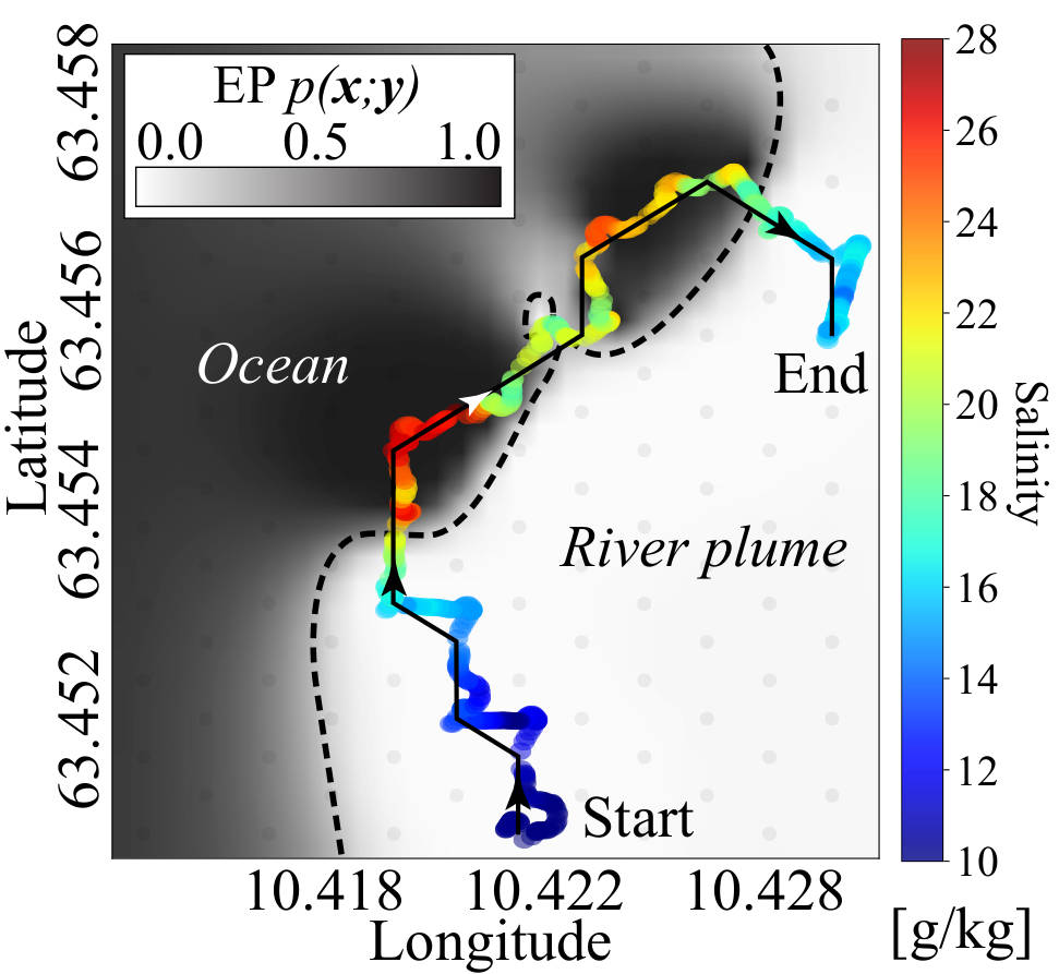
(c) Survey 1

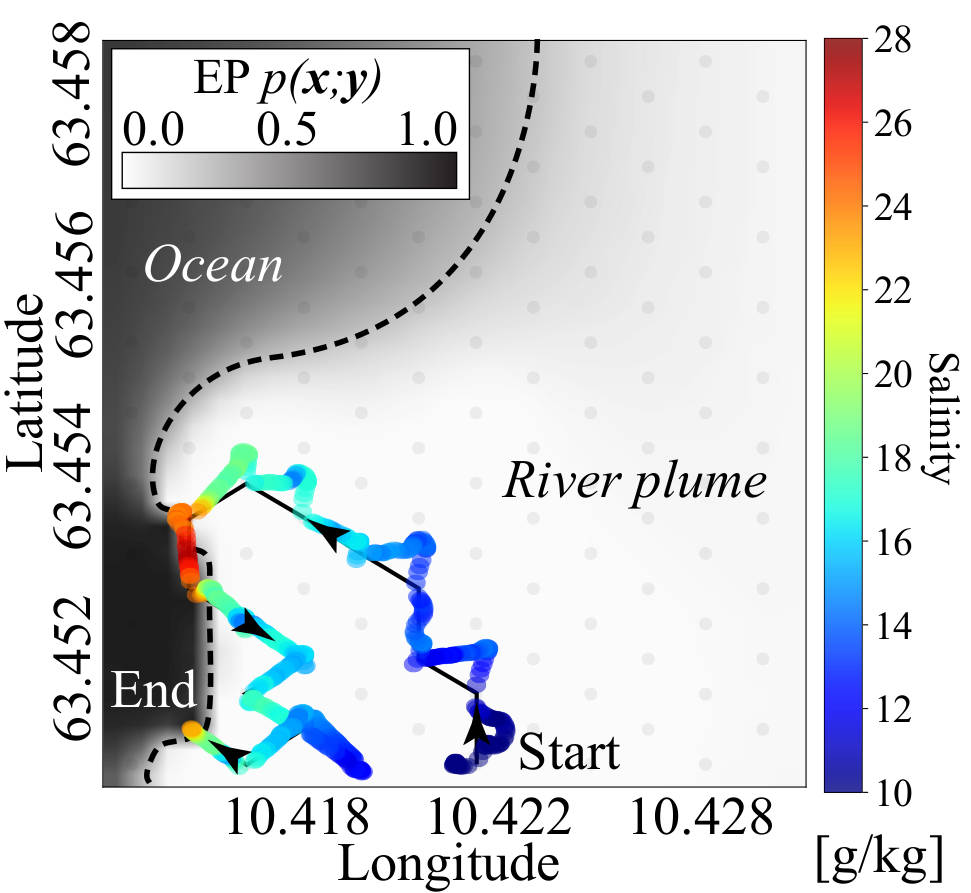
(d) Survey 2

Figure 11: Results from mapping the Nidelva river, Trondheim, Norway over two survey missions. 11(a) shows an overview of the survey area overlaid with the AUV path in black and dashed line. Note the shaded region indicating a typical frontal region. 11(b) shows the collected temperature data as colored trails. Note waypoint 5 (WP5) which indicates where the two surveys diverge. 11(c) and 11(d) shows the collected salinity data overlaid on the final EP, which indicate the AUVs statistical impression of the front. For both missions the temperature and salinity data correspond with an indication of the EP front. About 2 hours time separated the two runs.

4.3 Results

Two survey missions (1 and 2), were run successively, with a short break in between. The resulting path of the selected waypoints are shown in the map in Fig. 11(a), both within the expected frontal region (shaded pink). The recorded temperatures are shown as colored trails in Fig. 11(b), clearly indicating the temperature difference between fjord and riverine waters. The salinity data are then shown separately, overlaid with the estimated EP for each survey in Fig. 11(c) and Fig. 11(d).

Both surveys successfully estimated and navigated the separation zone, crossing the frontal boundary multiple times. As conditions changed slightly between the two surveys, the resulting trajectory (after waypoint 5) is shown to deviate. Survey 1 continued northwards, tracking the north-eastern portion of the front, while Survey 2 turned west, mapping the south-western region.

The final predictions of the front location, represented by conditional EPs in Fig. 11(c) and Fig. 11(d) as dashed lines, correspond with one another. In both surveys they yield a picture of the front being to the west in the southern portions of the region and gradually bending off toward the north east. The amount of exploration done by Survey 1 which turned north is greater than Survey 2 which was coming close to the survey area borders in the south-western corner.

5 Closing remarks

This work builds on a multidisciplinary effort combining statistical methods with robotic sampling for oceanographic applications. We show how observation practices can gain efficiency and accuracy from statistical techniques for spatial monitoring and demonstrate the the need for real-time multivariate spatial sampling on autonomous platforms.

In particular, we derive and show results for a real-world domain characterizing water mass properties. The characterization of uncertainties in random sets is extended in the vector-valued case with new results for the expected integrated Bernoulli variance reduction achieved by spatial sampling designs. This is provided in semi-analytical form for static designs, and then extended to the adaptive situations. The sequential derivations provide new insights into efficient applications of adaptive data collection, as demonstrated in our application.

The case study considers the upper water column in the river plume, represented by a two dimensional grid. Extensions to three-dimensional domains are not methodologically different, but likely approximate calculations by concentrating numerical integration on terms in the vicinity of the autonomous vehicle (Fossum et al., 2019). While we did not consider any temporal effects, which would be relevant on a larger time scale, we do consider the extension to spatio-temporal modeling and envision that advection-diffusion equations could be useful (Sigrist, Künsch and Stahel, 2015; Richardson, 2017). For more complex oceanographic phenomena, the methods will need to be extended to non-Gaussian phenomena, possibly feature-based mixtures of Gaussian processes which could potentially be run onboard augmented by dynamical models. Running numerical models onboard a robotic vehicle is currently infeasible, but high-resolution ocean models or remote sensing data can be used to fit a more complex statistical model Davidson et al. (2019).

The spatio-statistical design criterion building on random sets is relevant in our setting with different water properties. We show mathematical generality beyond the expected integrated Bernoulli variance, for instance, that of volume uncertainties which is possibly more relevant, but one that requires more computational resources. Such criteria could be particularly useful in other oceanographic settings related to mapping of algal-blooms, anoxic zones or open water fronts Costa et al. (2018). Other criteria could also be relevant, for instance, hybrid or multi-attribute criteria that could balance goals of exploration and exploitation in this situation. Equally, such techniques have significant use cases in downstream decision-making, with policy makers and regulators who need to make difficult decisions related to aquaculture or other marine resources. Value of information analysis (Eidsvik, Mukerji and Bhattacharjya, 2015) could be used to evaluate whether information is likely to result in improved decision-making, in such a context. We also foresee opportunities related to design of experiments for multivariate processes using our notion of generalized locations.

In our context the myopic strategy performs well, and due to computational constraints we did not go in depth on the dynamic programming solutions. There has been much work on finite horizon optimization in the robotics literature including probabilistic road maps and rapidly-exploring random trees (Karaman and Frazzoli, 2011), but their statistical properties are unclear. In some cases it is also limiting to use a waypoint graph, and would be beneficial to allow more continuous updates and navigation at the highest frequency possible given limitations being onboard an AUV. It is equally interesting to explore the additional flexibility that can be gained by having multiple vehicles co-temporally exploring a spatial or spatio-temporal domain (Ferreira et al., 2019). Such an approach would enable concurrent sampling in different parts of the space, or opportunities to move in parallel to best capture the excursion set. The value of information related to when and what to communicate (to shore or to other vehicles) is also an interesting thrust for research and likely to be useful for internet-of-things applications or computer experiments where some observations or evaluations are rather inexpensive, while others must only be done when they are really valuable.

Appendix

Proposition 3.

For a measurable random field $Z$ and a locally finite measure $\nu$ on $\mathcal{M}$, $\nu(\Gamma)$ is a random variable and for any $r\geq 1$,

$$\begin{split}\mathbb{E}[\nu(\Gamma)^{r}]&=\int_{\mathcal{M}^{r}}\mathbb{P}\left(Z_{\bm{u}}\in T^{r}\right)\mathrm{d}\nu^{\otimes}\left(\bm{u}\right),\end{split}$$

where the product measure is denoted as $\nu^{\otimes}:=\bigotimes_{i=1}^{r}\nu$. Here $Z$ is defined on $\mathcal{M}$, and for $\bm{u}=\left(u^{(1)},...,u^{(r)}\right)\in\mathcal{M}^{r}$, $Z_{\bm{u}}=\left(Z_{u^{(1)}},...,Z_{u^{(r)}}\right)\in\mathbb{R}^{pr}$.

In the particular case where $Z$ is a multivariate Gaussian random field we have

$$\mathbb{P}\left(Z_{\bm{u}}\in T^{r}\right)=\mathcal{N}_{pr}(T^{r};\mu(\bm{u}),K\left(\bm{u},\bm{u}\right))$$

where $\mathcal{N}_{pr}(\cdot;\mu(\bm{u}),K\left(\bm{u},\bm{u}\right))$ is the Gaussian measure on $\mathbb{R}^{pr}$ with mean $\mu(\bm{u})$ and covariance matrix $K\left(\bm{u},\bm{u}\right)$, respectively defined blockwise by

$$\mu(\bm{u}) =\begin{pmatrix}\mu(u^{(1)})\\ \vdots\\ \mu(u^{(r)})\end{pmatrix}\in\mathbb{R}^{pr},$$

$$\text{and }K\left(\bm{u},\bm{u}\right) =\begin{pmatrix}\operatorname{Cov}(Z_{u^{(1)}},Z_{u^{(1)}})&\dots&\operatorname{Cov}(Z_{u^{(1)}},Z_{u^{(r)}})\\ \vdots&&\vdots\\ \operatorname{Cov}(Z_{u^{(r)}},Z_{u^{(1)}})&\dots&\operatorname{Cov}(Z_{u^{(r)}},Z_{u^{(r)}})\\ \end{pmatrix}\in\mathbb{R}^{pr\times pr},$$

each of the $r\times r$ blocks of the latter matrix being itself a (cross-)covariance matrix of dimension $p\times p$. Assuming further that $K\left(\bm{u},\bm{u}\right)$ is non-singular, the probability of interest can be formulated in terms of the $pr$-dimensional Gaussian probability density function $\varphi_{pr}(\cdot;~{}\mu(\bm{u}),K\left(\bm{u},\bm{u}\right))$ as

$$\begin{split}&\mathbb{P}\left(Z_{\bm{u}}\in T^{r}\right)=\int_{T^{r}}\varphi_{pr}\left(\bm{v};~{}\mu(\bm{u}),K\left(\bm{u},\bm{u}\right)\right)\mathrm{d}\bm{v},\end{split}$$

In the particular orthant case with $T=(-\infty,t_{1}]\times\dots\times(-\infty,t_{r}]$, the latter probability directly writes in terms of the multivariate Gaussian cumulative distribution, this time by the way without requiring $K\left(\bm{u},\bm{u}\right)$ to be non-singular:

$$\begin{split}\mathbb{P}\left(Z_{\bm{u}}\in T^{r}\right)&=\varPhi_{pr}\left(\bm{t};~{}\mu(\bm{u}),K\left(\bm{u},\bm{u}\right)\right),\end{split}$$

where we have used the notations $t=(t_{1},\dots,t_{p})\in\mathbb{R}^{p}$, $1_{r}=(1,\dots,1)\in\mathbb{R}^{r}$, and $\bm{t}=1_{r}\otimes\bm{t}=(t_{1},\dots,t_{p},\dots,t_{1},\dots,t_{p})\in\mathbb{R}^{pr}$.

Proof.

That $\nu(\Gamma)$ defines indeed a random variable follows from Fubini’s theorem relying on the joint measurability of $(u,\omega)\to\mathbbm{1}_{\Gamma(\omega)}(u)$, itself inherited from the assumed measurability for $(u,\omega)\to Z_{u}(\omega)$ and $T$, respectively. From there, following the steps of Robbins’ theorem Robbins (1944), we find that

$$\begin{split}\mathbb{E}[\nu(\Gamma)^{r}]&=\mathbb{E}\left[\left(\int_{\mathcal{M}}\mathbbm{1}_{Z_{u}\in T}~{}d\nu(u)\right)^{r}\right]=\mathbb{E}\left[\prod_{i=1}^{r}\left(\int_{\mathcal{M}}\mathbbm{1}_{Z_{u^{(i)}}\in T}~{}d\nu(u^{(i)})\right)\right]\\ &=\mathbb{E}\left[\int_{\mathcal{M}^{r}}\mathbbm{1}_{Z_{u^{(1)}}\in T,\dots,Z_{u^{(r)}}\in T}\mathrm{d}\nu^{\otimes}\left(\bm{u}\right)\right]=\int_{\mathcal{M}^{r}}\mathbb{P}\left(Z_{\bm{u}}\in T^{r}\right)\mathrm{d}\nu^{\otimes}\left(\bm{u}\right).\end{split}$$

The rest consists in expliciting the probability of $T\times\dots\times T$ under the multivariate Gaussian distribution of $\left(Z_{u^{(1)}},\dots,Z_{u^{(r)}}\right)$. ∎

The propositions below provide formulae for computations of expectations of moments of multivariate gaussian CDFs.

Proposition 4.

Let $p,q,h\geq 1$, $a\in\mathbb{R}^{p}$, $B\in\mathbb{R}^{p\times q}$, and $C$, $C_{V}$ be two covariance matrices in $\mathbb{R}^{p\times p}$ and $\mathbb{R}^{q\times q}$, respectively. Then, for $V\sim\mathcal{N}_{q}(0_{q},C_{V})$,

$$\mathbb{E}\left[\varPhi_{p}\left(a+BV;C\right)^{h}\right]=\varPhi_{ph}\left(\bm{a};~{}\bm{\Sigma}\right),$$

where the vector $\bm{a}\in\mathbb{R}^{ph}$ is defined as $\bm{a}:=1_{h}\otimes a=\left(a,\dots,a\right)^{\prime}$ and the $ph\times ph$ covariance matrix is given by $\bm{\Sigma}:=1_{h}1_{h}^{\prime}\otimes BC_{V}B^{\prime}+I_{h}\otimes C$.

Remark 1.

In blockwise representation, $\bm{\Sigma}$ can be expressed as follows:

$$\begin{pmatrix}C&&\\ &\ddots&\\ &&C\end{pmatrix}+\begin{pmatrix}BC_{V}B^{\prime}&\dots&BC_{V}B^{\prime}\\ \vdots&&\vdots\\ BC_{V}B^{\prime}&\dots&BC_{V}B^{\prime}\\ \end{pmatrix}$$

Proof.

By definition of $\Phi_{p}$, for $N\sim\mathcal{N}_{p}(0_{p},C)$,

$$\mathbb{P}(N\leq a+BV|V)=\varPhi_{p}\left(a+BV;C\right).$$

Now for $\varPhi_{p}\left(a+BV;C\right)^{h}$, provided that the probability space is sufficiently large to accomodate $h$ independent Gaussian random vectors $N_{i}\sim\mathcal{N}_{p}(0,C)$ (which is silently assumed here), using the former equality delivers

$$\varPhi_{p}\left(a+BV;C\right)^{h}=\prod_{i=1}^{h}\mathbb{P}(N_{i}\leq a+BV|V).$$

Now by independence of the $N_{i}$’s we obtain the joint conditional probability

$$\prod_{i=1}^{h}\mathbb{P}(N_{i}\leq a+BV|V)=\mathbb{P}(N_{1}\leq a+BV,\dots,N_{h}\leq a+BV|V),$$

whereof, by virtue of the law of total expectation,

$$\begin{split}\mathbb{E}\left[\varPhi_{p}\left(a+BV;C\right)^{h}\right]&=\mathbb{E}\left[\mathbb{P}(N_{1}\leq a+BV,\dots,N_{h}\leq a+BV|V)\right]\\ &=\mathbb{P}(N_{1}\leq a+BV,\dots,N_{h}\leq a+BV)\\ &=\mathbb{P}(W_{1}\leq a,\dots,W_{h}\leq a)\\ &=\varPhi_{ph}\left(1_{h}\otimes a;(1_{h}1_{h}^{\prime})\otimes(B\Sigma_{V}B^{\prime})+I_{h}\otimes C\right),\end{split}$$

where $\mathbf{W}=(W_{1},\dots,W_{h})$ with $W_{i}=N_{i}-BV\ (1\leq i\leq h)$ and the last line follows $\mathbf{W}$ forming a Gaussian vector (by global independence of the $N_{i}$’s and $V$) and from the definition of $\varPhi_{ph}$. The covariance matrix $\mathbf{\Sigma}$ of $\mathbf{W}$ is obtained by noting that $\operatorname{cov}(W_{i},W_{j})=BC_{V}B^{\prime}+\delta_{ij}C\ (i,j\in\{1,\dots,h\})$. ∎

We now generalize Proposition 4 to the case of multivariate monomials in orthant probabilities with thresholds affine in a common Gaussian vector.

Proposition 5.

Let $g,p,q\geq 1$, $h_{1},\dots,h_{g}\geq 1$ with $H=\sum_{i=1}^{g}h_{i}$, $a_{i}\in\mathbb{R}^{p}$, $B_{i}\in\mathbb{R}^{p\times q}$, and covariance matrices $C_{i}\in\mathbb{R}^{p\times p}$ $(1\leq i\leq g)$. Then, for any covariance matrix $C_{V}\in\mathbb{R}^{q\times q}$ and $V\sim\mathcal{N}_{q}(0_{q},C_{V})$,

$$\mathbb{E}\left[\prod_{i=1}^{g}\varPhi_{p}\left(a_{i}+B_{i}V;C_{i}\right)^{h_{i}}\right]=\varPhi_{pH}\left(\bm{a};\mathbf{\Sigma}\right),$$ (20)

with $\bm{a}=(1_{h_{1}}\otimes a_{1},\dots,1_{h_{g}}\otimes a_{g})\in\mathbb{R}^{pH}$ and $\mathbf{\Sigma}\in\mathbb{R}^{pH\times pH}$ is defined blockwise by $(\Sigma_{i,j})_{i,j\in\{1,\dots,g\}}$ where, for any $i,j\in\{1,\dots,g\}$,

$$\Sigma_{i,j}=(1_{h_{i}}1_{h_{j}}^{\prime})\otimes(B_{i}\Sigma_{V}B_{j}^{\prime})+\delta_{i,j}(I_{h_{i}}\otimes C_{i})\in\mathbb{R}^{ph_{i}\times ph_{j}}.$$ (21)

Remark 2.

Using blockwise representation for the blocks themselves delivers

$$\Sigma_{ij}=\begin{pmatrix}B_{i}\Sigma_{V}B_{j}^{\prime}&\dots&B_{i}\Sigma_{V}B_{j}^{\prime}\\ \vdots&&\vdots\\ B_{i}\Sigma_{V}B_{j}^{\prime}&\dots&B_{i}\Sigma_{V}B_{j}^{\prime}\\ \end{pmatrix}+\delta_{ij}\begin{pmatrix}C_{i}&&\\ &\ddots&\\ &&C_{i}\end{pmatrix}$$

Here each $\Sigma_{ij}$ is made of $h_{i}$ times $h_{j}$ (vertically/horizontally) $p\times p$ sub-blocks, hence possesses $ph_{i}$ lines and $ph_{j}$ columns.

Proof.

The proof relies (again) heavily on the fact that, by definition of $\Phi_{p}$, for any covariance matrix $C\in\mathbb{R}^{p\times p}$, $a\in\mathbb{R}^{p}$, $B\in\mathbb{R}^{p\times q}$, and $N\sim\mathcal{N}_{p}(0_{p},C)$,

$$\mathbb{P}(N\leq a+BV|V)=\varPhi_{p}\left(a+BV;C\right).$$

In particular, for globally independent $N_{i,j}\sim\mathcal{N}_{p}(0_{p},C_{i})$ $(1\leq j\leq h_{i},1\leq i\leq g)$,

$$\begin{split}\prod_{i=1}^{g}\varPhi_{p}\left(a_{i}+B_{i}V;C_{i}\right)^{h_{i}}&=\prod_{i=1}^{g}\prod_{j=1}^{h_{i}}\mathbb{P}(N_{i,j}\leq a_{i}+B_{i}V|V)\\ &=\mathbb{P}(N_{1,1}\leq a_{1}+B_{1}V,\dots,N_{g,h_{g}}\leq a_{g}+B_{g}V|V),\end{split}$$

so that, by the law of total expectation,

$$\begin{split}\mathbb{E}\left[\prod_{i=1}^{g}\varPhi_{p}\left(a_{i}+B_{i}V;C_{i}\right)^{h_{i}}\right]=\mathbb{P}(W_{1}\leq 1_{h_{1}}\otimes a_{1},\dots,W_{g}\leq 1_{h_{g}}\otimes a_{g})\end{split}$$

where $W_{1}=(N_{1,1}-B_{1}V,\dots,N_{1,h_{1}}-B_{1}V),W_{2}=(N_{2,1}-B_{2}V,\dots,N_{2,h_{2}}-B_{2}V),\dots,W_{g}=(N_{g,1}-B_{g}V,\dots,N_{g,h_{g}}-B_{g}V)$. Noting that $\mathbf{W}=(W_{1},\dots,W_{g})$ is a centred $pH$-dimensional Gaussian random vector, we finally obtain that

$$\begin{split}\mathbb{E}\left[\prod_{i=1}^{g}\varPhi_{p}\left(a_{i}+B_{i}V;C_{i}\right)^{h_{i}}\right]=\varPhi_{pH}\left(\bm{a};\mathbf{\Sigma}\right),\end{split}$$

with $\bm{a}=(1_{h_{1}}\otimes a_{1},\dots,1_{h_{g}}\otimes a_{g})$ and $\bm{\Sigma}=(\operatorname{cov}(W_{i},W_{j}))_{i,j\in\{1,\dots,g\}}$. ∎

Those two general results allow us to derive simple expressions for the expected effect of the inclusion of new datapoints on the $\operatorname{IBV}$ (Proposition 1) and on the $\operatorname{EMV}$ (Proposition 2) for which we provide proofs below.

Proof.

(Proposition 1) Applying Tonelli-Fubini followed by the law of total expectation first delivers

$$\begin{split}\mathrm{EIBV}_{[n]}(\bm{x})&=\int_{\mathcal{M}}\mathbb{E}_{[n]}\left[\mathbb{P}_{[n+1]}\left(Z_{u}\in T\right)(1-\mathbb{P}_{[n+1]}\left(Z_{u}\in T\right))\right]d\nu(u)\\ &=\int_{\mathcal{M}}\varPhi_{p}\left({\bm{t}};~{}\mu_{[n+1]}\left(u\right),K_{[n+1]}\left(u,u\right)\right)d\nu(u)\\ &-\int_{\mathcal{M}}\mathbb{E}_{[n]}\left[\varPhi_{p}\left({\bm{t}};~{}\mu_{[n+1]}\left(u\right),K_{[n+1]}\left(u,u\right)\right)^{2}\right]d\nu(u),\end{split}$$

where $K_{[n+1]}\left(u,u\right)$ denotes the $p\times p$ covariance matrix between all $p$ responses at point $u$ conditional on the first $n+1$ observation batches. Now, by using co-kriging update formulae and our shortcut notation for the CDF of centred multivariate Gaussian vectors, we observe that

$$\begin{split}&\varPhi_{p}\left({\bm{t}};~{}\mu_{[n+1]}\left(u\right),K_{[n+1]}\left(u,u\right)\right)\\ =&\varPhi_{p}\left({\bm{t}}-\mu_{[n+1]}\left(u\right);K_{[n+1]}\left(u,u\right)\right)\\ =&\varPhi_{p}\left({\bm{t}}-\mu_{[n]}\left(u\right)-\lambda_{[n+1,n+1]}(u)^{T}(Z_{\bm{x}_{n+1}}-\mu_{[n]}\left(\bm{x}_{n+1}\right)),K_{[n+1]}\left(u,u\right)\right)\\ =&\varPhi_{p}\left(a+BV,K_{[n+1]}\left(u,u\right)\right),\end{split}$$

with $a={\bm{t}}-\mu_{[n]}\left(u\right)$, $B=-\lambda_{[n+1,n+1]}(u)^{T}$ and $V=Z_{\bm{x}_{n+1}}-\mu_{[n]}\left(\bm{x}_{n+1}\right)$. Applying Proposition 4 then delivers that

$$\begin{split}&\mathbb{E}_{[n]}\left[\varPhi_{p}\left({\bm{t}};~{}\mu_{[n+1]}\left(u\right),K_{[n+1]}\left(u,u\right)\right)^{2}\right]=\varPhi_{2p}\left(\left(\begin{matrix}{\bm{t}}-\mu_{[n]}\left(u\right)\\ {\bm{t}}-\mu_{[n]}\left(u\right)\end{matrix}\right);\mathbf{\Sigma}_{[n]}(u)\right),\end{split}$$

with $\mathbf{\Sigma}_{[n]}(u)$ as in the formulation of the proposition. This completes the proof. ∎

Proof.

(Proposition 2)

$$\begin{split}\operatorname{EEMV}_{[n]}(\bm{x})&=\int_{\mathcal{M}^{2}}\varPhi_{2p}\left(({\bm{t}},{\bm{t}});\mu((u,v)),K((u,v),(u,v))\right)\ \mathrm{d}\nu^{\otimes}(u,v)\\ &-\int_{\mathcal{M}^{2}}\mathbb{E}_{[n]}\left[\varPhi_{p}\left({\bm{t}};\mu_{[n+1]}\left(u\right),K_{[n+1]}(u,u)\right)\varPhi_{p}\left({\bm{t}};\mu_{[n+1]}\left(v\right),K_{[n+1]}(v,v)\right)\right]\ \mathrm{d}\nu^{\otimes}(u,v)\end{split}$$

and the proof follows by applying Proposition 5 with

$$V=Z_{\bm{x}_{n+1}}-\mu_{[n]}\left(\bm{x}_{n+1}\right)\sim\mathcal{N}(0_{q_{n+1}},k_{[n]}(\bm{x}_{n+1},\bm{x}_{n+1}))$$

and $a_{1}={\bm{t}}-\mu_{[n]}\left(u\right)$, $B_{1}=-\lambda_{[n+1,n+1]}(u)^{T}$, $a_{2}={\bm{t}}-\mu_{[n]}\left(v\right)$, $B_{2}=-\lambda_{[n+1,n+1]}(v)^{T}$, $C_{1}=K_{[n]}\left(u,u\right)$, $C_{2}=K_{[n]}\left(v,v\right)$. ∎

References

- Costa et al. (2018) {binproceedings}[author] \bauthor\bsnmCosta, \bfnmMaria João\binitsM. J., \bauthor\bsnmPinto, \bfnmJose\binitsJ., \bauthor\bsnmDias, \bfnmPaulo Sousa\binitsP. S., \bauthor\bsnmPereira, \bfnmJoão\binitsJ., \bauthor\bsnmLima, \bfnmKeila\binitsK., \bauthor\bsnmRibeiro, \bfnmManuel\binitsM., \bauthor\bsnmSousa, \bfnmJoão Borges\binitsJ. B., \bauthor\bsnmLukaczyk, \bfnmTrent\binitsT., \bauthor\bsnmMendes, \bfnmRenato\binitsR., \bauthor\bsnmTomasino, \bfnmMaria P.\binitsM. P., \bauthor\bsnmMagahlaes, \bfnmCatarina\binitsC., \bauthor\bsnmBelkin, \bfnmIgor\binitsI., \bauthor\bsnmLopez-Castejon, \bfnmFrancisco\binitsF., \bauthor\bsnmGilabert, \bfnmJavier\binitsJ., \bauthor\bsnmSkarpnes, \bfnmKay Arne\binitsK. A., \bauthor\bsnmLudvigsen, \bfnmMartin\binitsM., \bauthor\bsnmRajan, \bfnmKanna\binitsK., \bauthor\bsnmMirmalek, \bfnmZara\binitsZ. and \bauthor\bsnmChekalyuk, \bfnmAlex\binitsA. (\byear2018). \btitleField Report: Exploring Fronts with Multiple Robots. In \bbooktitleIEEE AUV. \endbibitem
- Azzimonti et al. (2016) {barticle}[author] \bauthor\bsnmAzzimonti, \bfnmD.\binitsD., \bauthor\bsnmBect, \bfnmJ.\binitsJ., \bauthor\bsnmChevalier, \bfnmC.\binitsC. and \bauthor\bsnmGinsbourger, \bfnmD.\binitsD. (\byear2016). \btitleQuantifying and reducing uncertainties on excursion sets under a Gaussian field prior. \bjournalSIAM/ASA Journal on Uncertainty Quantification \bvolume4(1) \bpages850-874. \endbibitem
- Azzimonti et al. (2019) {barticle}[author] \bauthor\bsnmAzzimonti, \bfnmD.\binitsD., \bauthor\bsnmGinsbourger, \bfnmD.\binitsD., \bauthor\bsnmChevalier, \bfnmC.\binitsC., \bauthor\bsnmBect, \bfnmJ.\binitsJ. and \bauthor\bsnmRichet, \bfnmY.\binitsY. (\byear2019). \btitleAdaptive Design of Experiments for Conservative Estimation of Excursion Sets. \bjournalTechnometrics (Published online). \endbibitem
- Bect, Bachoc and Ginsbourger (2019) {barticle}[author] \bauthor\bsnmBect, \bfnmJulien\binitsJ., \bauthor\bsnmBachoc, \bfnmFrançois\binitsF. and \bauthor\bsnmGinsbourger, \bfnmDavid\binitsD. (\byear2019). \btitleA supermartingale approach to Gaussian process based sequential design of experiments. \bjournalBernoulli \bvolume25 \bpages2883–2919. \endbibitem
- Bect et al. (2012) {barticle}[author] \bauthor\bsnmBect, \bfnmJ.\binitsJ., \bauthor\bsnmGinsbourger, \bfnmD.\binitsD., \bauthor\bsnmLi, \bfnmL.\binitsL., \bauthor\bsnmPicheny, \bfnmV.\binitsV. and \bauthor\bsnmVazquez, \bfnmE.\binitsE. (\byear2012). \btitleSequential design of computer experiments for the estimation of a probability of failure. \bjournalStatistics and Computing \bvolume22 (3) \bpages773-793. \endbibitem
- Bellingham and Rajan (2007) {barticle}[author] \bauthor\bsnmBellingham, \bfnmJ. G.\binitsJ. G. and \bauthor\bsnmRajan, \bfnmK.\binitsK. (\byear2007). \btitleRobotics in Remote and Hostile Environments. \bjournalScience \bvolume318 \bpages1098-1102. \endbibitem
- Bhattacharjya, Eidsvik and Mukerji (2013) {barticle}[author] \bauthor\bsnmBhattacharjya, \bfnmDebarun\binitsD., \bauthor\bsnmEidsvik, \bfnmJo\binitsJ. and \bauthor\bsnmMukerji, \bfnmTapan\binitsT. (\byear2013). \btitleThe value of information in portfolio problems with dependent projects. \bjournalDecision Analysis \bvolume10 \bpages341–351. \endbibitem
- Binney, Krause and Sukhatme (2013) {barticle}[author] \bauthor\bsnmBinney, \bfnmJ.\binitsJ., \bauthor\bsnmKrause, \bfnmA.\binitsA. and \bauthor\bsnmSukhatme, \bfnmG. S.\binitsG. S. (\byear2013). \btitleOptimizing waypoints for monitoring spatiotemporal phenomena. \bjournalThe International Journal of Robotics Research \bvolume32 \bpages873–888. \bdoi10.1177/0278364913488427 \endbibitem
- Bolin and Lindgren (2015) {barticle}[author] \bauthor\bsnmBolin, \bfnmD.\binitsD. and \bauthor\bsnmLindgren, \bfnmF.\binitsF. (\byear2015). \btitleExcursion and contour uncertainty regions for latent Gaussian models. \bjournalJournal of the Royal Statistical Society, Series B Methodology \bvolume77(1) \bpages85-106. \endbibitem
- Bueso, Angulo and Alonso (1998) {barticle}[author] \bauthor\bsnmBueso, \bfnmMC\binitsM., \bauthor\bsnmAngulo, \bfnmJM\binitsJ. and \bauthor\bsnmAlonso, \bfnmFJ\binitsF. (\byear1998). \btitleA state-space model approach to optimum spatial sampling design based on entropy. \bjournalEnvironmental and Ecological Statistics \bvolume5 \bpages29–44. \endbibitem
- Chevalier, Emery and Ginsbourger (2015) {barticle}[author] \bauthor\bsnmChevalier, \bfnmC.\binitsC., \bauthor\bsnmEmery, \bfnmX.\binitsX. and \bauthor\bsnmGinsbourger, \bfnmD.\binitsD. (\byear2015). \btitleFast update of conditional simulation ensembles. \bjournalMathematical geosciences \bvolume47 \bpages771-789. \endbibitem
- Chevalier, Ginsbourger and Emery (2013) {binproceedings}[author] \bauthor\bsnmChevalier, \bfnmC.\binitsC., \bauthor\bsnmGinsbourger, \bfnmD.\binitsD. and \bauthor\bsnmEmery, \bfnmX.\binitsX. (\byear2013). \btitleCorrected Kriging Update Formulae for Batch-Sequential Data Assimilation. In \bbooktitleMathematics of Planet Earth (\beditor\bfnmE.\binitsE. \bsnmPardo-Igúzquiza, \beditor\bfnmC.\binitsC. \bsnmGuardiola-Albert, \beditor\bfnmJ.\binitsJ. \bsnmHeredia, \beditor\bfnmL.\binitsL. \bsnmMoreno-Merino, \beditor\bfnmJ.\binitsJ. \bsnmDurán and \beditor\bfnmJ.\binitsJ. \bsnmVargas-Guzmán, eds.). \bseriesLecture Notes in Earth System Sciences. \bpublisherSpringer, Berlin, Heidelberg. \endbibitem
- Chevalier et al. (2013) {bincollection}[author] \bauthor\bsnmChevalier, \bfnmC.\binitsC., \bauthor\bsnmGinsbourger, \bfnmD.\binitsD., \bauthor\bsnmBect, \bfnmJ.\binitsJ. and \bauthor\bsnmMolchanov, \bfnmI.\binitsI. (\byear2013). \btitleEstimating and quantifying uncertainties on level sets using the Vorob’ev expectation and deviation with Gaussian process models. In \bbooktitlemODa 10 Advances in Model-Oriented Design and Analysis (\beditor\bfnmD.\binitsD. \bsnmUciński, \beditor\bfnmA. C.\binitsA. C. \bsnmAtkinson and \beditor\bfnmC.\binitsC. \bsnmPatan, eds.) \bpublisherPhysica-Verlag HD. \endbibitem
- Chevalier et al. (2014) {barticle}[author] \bauthor\bsnmChevalier, \bfnmClément\binitsC., \bauthor\bsnmBect, \bfnmJulien\binitsJ., \bauthor\bsnmGinsbourger, \bfnmDavid\binitsD., \bauthor\bsnmVazquez, \bfnmEmmanuel\binitsE., \bauthor\bsnmPicheny, \bfnmVictor\binitsV. and \bauthor\bsnmRichet, \bfnmYann\binitsY. (\byear2014). \btitleFast parallel kriging-based stepwise uncertainty reduction with application to the identification of an excursion set. \bjournalTechnometrics \bvolume56 \bpages455–465. \endbibitem
- Das et al. (2012) {barticle}[author] \bauthor\bsnmDas, \bfnmJ.\binitsJ., \bauthor\bsnmPy, \bfnmF.\binitsF., \bauthor\bsnmMaughan, \bfnmT.\binitsT., \bauthor\bsnmMessie, \bfnmM.\binitsM., \bauthor\bsnmO’Reilly, \bfnmT.\binitsT., \bauthor\bsnmRyan, \bfnmJ.\binitsJ., \bauthor\bsnmSukhatme, \bfnmG. S.\binitsG. S. and \bauthor\bsnmRajan, \bfnmK.\binitsK. (\byear2012). \btitleCoordinated Sampling of Dynamic Oceanographic Features with AUVs and Drifters. \bjournalInternational Journal of Robotics Research \bvolume31 \bpages626-646. \bnoteApril. \endbibitem
- Das et al. (2015) {barticle}[author] \bauthor\bsnmDas, \bfnmJnaneshwar\binitsJ., \bauthor\bsnmPy, \bfnmFrederic\binitsF., \bauthor\bsnmHarvey, \bfnmJulio B. J.\binitsJ. B. J., \bauthor\bsnmRyan, \bfnmJohn P.\binitsJ. P., \bauthor\bsnmGellene, \bfnmAlyssa\binitsA., \bauthor\bsnmGraham, \bfnmRishi\binitsR., \bauthor\bsnmCaron, \bfnmDavid A.\binitsD. A., \bauthor\bsnmRajan, \bfnmKanna\binitsK. and \bauthor\bsnmSukhatme, \bfnmGaurav S.\binitsG. S. (\byear2015). \btitleData-driven robotic sampling for marine ecosystem monitoring. \bjournalThe International Journal of Robotics Research \bvolume34 \bpages1435–1452. \bdoi10.1177/0278364915587723 \endbibitem
- Davidson et al. (2019) {barticle}[author] \bauthor\bsnmDavidson, \bfnmFraser\binitsF., \bauthor\bsnmAlvera-Azcárate, \bfnmAida\binitsA., \bauthor\bsnmBarth, \bfnmAlexander\binitsA., \bauthor\bsnmBrassington, \bfnmGary B.\binitsG. B., \bauthor\bsnmChassignet, \bfnmEric P.\binitsE. P., \bauthor\bsnmClementi, \bfnmEmanuela\binitsE., \bauthor\bsnmDe Mey-Frémaux, \bfnmPierre\binitsP., \bauthor\bsnmDivakaran, \bfnmPrasanth\binitsP., \bauthor\bsnmHarris, \bfnmChristopher\binitsC., \bauthor\bsnmHernandez, \bfnmFabrice\binitsF., \bauthor\bsnmHogan, \bfnmPatrick\binitsP., \bauthor\bsnmHole, \bfnmLars R.\binitsL. R., \bauthor\bsnmHolt, \bfnmJason\binitsJ., \bauthor\bsnmLiu, \bfnmGuimei\binitsG., \bauthor\bsnmLu, \bfnmYouyu\binitsY., \bauthor\bsnmLorente, \bfnmPablo\binitsP., \bauthor\bsnmMaksymczuk, \bfnmJan\binitsJ., \bauthor\bsnmMartin, \bfnmMatthew\binitsM., \bauthor\bsnmMehra, \bfnmAvichal\binitsA., \bauthor\bsnmMelsom, \bfnmArne\binitsA., \bauthor\bsnmMo, \bfnmHuier\binitsH., \bauthor\bsnmMoore, \bfnmAndrew\binitsA., \bauthor\bsnmOddo, \bfnmPaolo\binitsP., \bauthor\bsnmPascual, \bfnmAnanda\binitsA., \bauthor\bsnmPequignet, \bfnmAnne-Christine\binitsA.-C., \bauthor\bsnmKourafalou, \bfnmVilly\binitsV., \bauthor\bsnmRyan, \bfnmAndrew\binitsA., \bauthor\bsnmSiddorn, \bfnmJohn\binitsJ., \bauthor\bsnmSmith, \bfnmGregory\binitsG., \bauthor\bsnmSpindler, \bfnmDeanna\binitsD., \bauthor\bsnmSpindler, \bfnmTodd\binitsT., \bauthor\bsnmStanev, \bfnmEmil V.\binitsE. V., \bauthor\bsnmStaneva, \bfnmJoanna\binitsJ., \bauthor\bsnmStorto, \bfnmAndrea\binitsA., \bauthor\bsnmTanajura, \bfnmClemente\binitsC., \bauthor\bsnmVinayachandran, \bfnmP. N.\binitsP. N., \bauthor\bsnmWan, \bfnmLiying\binitsL., \bauthor\bsnmWang, \bfnmHui\binitsH., \bauthor\bsnmZhang, \bfnmYu\binitsY., \bauthor\bsnmZhu, \bfnmXueming\binitsX. and \bauthor\bsnmZu, \bfnmZiqing\binitsZ. (\byear2019). \btitleSynergies in Operational Oceanography: The Intrinsic Need for Sustained Ocean Observations. \bjournalFrontiers in Marine Science \bvolume6 \bpages450. \bdoi10.3389/fmars.2019.00450 \endbibitem
- Eidsvik, Mukerji and Bhattacharjya (2015) {bbook}[author] \bauthor\bsnmEidsvik, \bfnmJo\binitsJ., \bauthor\bsnmMukerji, \bfnmTapan\binitsT. and \bauthor\bsnmBhattacharjya, \bfnmDebarun\binitsD. (\byear2015). \btitleValue of Information in the Earth Sciences: Integrating Spatial Modeling and Decision Analysis. \bpublisherCambridge University Press, \baddressCambridge. \bdoi10.1017/CBO9781139628785 \endbibitem
- Ferreira et al. (2019) {barticle}[author] \bauthor\bsnmFerreira, \bfnmAntónio Sérgio\binitsA. S., \bauthor\bsnmCosta, \bfnmMaria\binitsM., \bauthor\bsnmPy, \bfnmFrédéric\binitsF., \bauthor\bsnmPinto, \bfnmJosé\binitsJ., \bauthor\bsnmSilva, \bfnmMónica A\binitsM. A., \bauthor\bsnmNimmo-Smith, \bfnmAlex\binitsA., \bauthor\bsnmJohansen, \bfnmTor Arne\binitsT. A., \bauthor\bparticlede \bsnmSousa, \bfnmJoão Borges\binitsJ. B. and \bauthor\bsnmRajan, \bfnmKanna\binitsK. (\byear2019). \btitleAdvancing multi-vehicle deployments in oceanographic field experiments. \bjournalAutonomous Robots \bvolume43 \bpages1555–1574. \endbibitem
- Fossum et al. (2018) {barticle}[author] \bauthor\bsnmFossum, \bfnmTrygve Olav\binitsT. O., \bauthor\bsnmEidsvik, \bfnmJo\binitsJ., \bauthor\bsnmEllingsen, \bfnmIngrid\binitsI., \bauthor\bsnmAlver, \bfnmMorten Omholt\binitsM. O., \bauthor\bsnmFragoso, \bfnmGlaucia Moreira\binitsG. M., \bauthor\bsnmJohnsen, \bfnmGeir\binitsG., \bauthor\bsnmMendes, \bfnmRenato\binitsR., \bauthor\bsnmLudvigsen, \bfnmMartin\binitsM. and \bauthor\bsnmRajan, \bfnmKanna\binitsK. (\byear2018). \btitleInformation-driven robotic sampling in the coastal ocean. \bjournalJournal of Field Robotics \bvolume35 \bpages1101-1121. \bdoi10.1002/rob.21805 \endbibitem
- Fossum et al. (2019) {barticle}[author] \bauthor\bsnmFossum, \bfnmTrygve Olav\binitsT. O., \bauthor\bsnmFragoso, \bfnmGlaucia M.\binitsG. M., \bauthor\bsnmDavies, \bfnmEmlyn J.\binitsE. J., \bauthor\bsnmUllgren, \bfnmJenny E.\binitsJ. E., \bauthor\bsnmMendes, \bfnmRenato\binitsR., \bauthor\bsnmJohnsen, \bfnmGeir\binitsG., \bauthor\bsnmEllingsen, \bfnmIngrid\binitsI., \bauthor\bsnmEidsvik, \bfnmJo\binitsJ., \bauthor\bsnmLudvigsen, \bfnmMartin\binitsM. and \bauthor\bsnmRajan, \bfnmKanna\binitsK. (\byear2019). \btitleToward adaptive robotic sampling of phytoplankton in the coastal ocean. \bjournalScience Robotics \bvolume4. \bdoi10.1126/scirobotics.aav3041 \endbibitem
- French and Sain (2013) {barticle}[author] \bauthor\bsnmFrench, \bfnmJ. P.\binitsJ. P. and \bauthor\bsnmSain, \bfnmS. R.\binitsS. R. (\byear2013). \btitleSpatio-temporal exceedance locations and confidence regions. \bjournalAnnals of Applied Statistics \bvolume7 (3) \bpages1421-1449. \endbibitem
- Genton and Kleiber (2015) {barticle}[author] \bauthor\bsnmGenton, \bfnmMarc G\binitsM. G. and \bauthor\bsnmKleiber, \bfnmWilliam\binitsW. (\byear2015). \btitleCross-covariance functions for multivariate geostatistics. \bjournalStatistical Science \bvolume30 \bpages147–163. \endbibitem
- Genz and Bretz (2009) {bbook}[author] \bauthor\bsnmGenz, \bfnmAlan\binitsA. and \bauthor\bsnmBretz, \bfnmFrank\binitsF. (\byear2009). \btitleComputation of multivariate normal and t probabilities \bvolume195. \bpublisherSpringer Science & Business Media. \endbibitem
- Ginsbourger (2018) {binbook}[author] \bauthor\bsnmGinsbourger, \bfnmD.\binitsD. (\byear2018). \btitleWiley StatsRef: Statistics Reference Online \bchapterSequential Design of Computer Experiments, \bpages1-9. \endbibitem
- Gneiting, Kleiber and Schlather (2010) {barticle}[author] \bauthor\bsnmGneiting, \bfnmTilmann\binitsT., \bauthor\bsnmKleiber, \bfnmWilliam\binitsW. and \bauthor\bsnmSchlather, \bfnmMartin\binitsM. (\byear2010). \btitleMatérn cross-covariance functions for multivariate random fields. \bjournalJournal of the American Statistical Association \bvolume105 \bpages1167–1177. \endbibitem
- Gottlieb et al. (2012) {binproceedings}[author] \bauthor\bsnmGottlieb, \bfnmJ.\binitsJ., \bauthor\bsnmGraham, \bfnmR.\binitsR., \bauthor\bsnmMaughan, \bfnmT.\binitsT., \bauthor\bsnmPy, \bfnmF.\binitsF., \bauthor\bsnmElkaim, \bfnmG.\binitsG. and \bauthor\bsnmRajan, \bfnmK.\binitsK. (\byear2012). \btitleAn Experimental Momentum-based Front Detection for Autonomous Underwater Vehicles. In \bbooktitleIEEE International Conference on Robotics and Automation (ICRA). \endbibitem
- Hopkins et al. (2013) {barticle}[author] \bauthor\bsnmHopkins, \bfnmJo\binitsJ., \bauthor\bsnmLucas, \bfnmMarc\binitsM., \bauthor\bsnmDufau, \bfnmClaire\binitsC., \bauthor\bsnmSutton, \bfnmMarion\binitsM., \bauthor\bsnmStum, \bfnmJacques\binitsJ., \bauthor\bsnmLauret, \bfnmOlivier\binitsO. and \bauthor\bsnmChannelliere, \bfnmClaire\binitsC. (\byear2013). \btitleDetection and variability of the Congo River plume from satellite derived sea surface temperature, salinity, ocean colour and sea level. \bjournalRemote sensing of environment \bvolume139 \bpages365–385. \endbibitem
- Karaman and Frazzoli (2011) {barticle}[author] \bauthor\bsnmKaraman, \bfnmSertac\binitsS. and \bauthor\bsnmFrazzoli, \bfnmEmilio\binitsE. (\byear2011). \btitleSampling-based algorithms for optimal motion planning. \bjournalThe international journal of robotics research \bvolume30 \bpages846–894. \endbibitem
- Krige (1951) {barticle}[author] \bauthor\bsnmKrige, \bfnmD. G.\binitsD. G. (\byear1951). \btitleA statistical approach to some basic mine valuation problems on the witwatersrand. \bjournalJ. of the Chem., Metal. and Mining Soc. of South Africa \bvolume52 \bpages119-139. \endbibitem
- Le Gratiet, Cannamela and Iooss (2015) {barticle}[author] \bauthor\bsnmLe Gratiet, \bfnmL.\binitsL., \bauthor\bsnmCannamela, \bfnmC.\binitsC. and \bauthor\bsnmIooss, \bfnmB.\binitsB. (\byear2015). \btitleCokriging-based sequential design strategies using fast cross-validation for multi-fidelity computer codes. \bjournalTechnometrics \bvolume57 \bpages418-427. \endbibitem
- Lermusiaux (2006) {barticle}[author] \bauthor\bsnmLermusiaux, \bfnmPierre F. J.\binitsP. F. J. (\byear2006). \btitleUncertainty Estimation and Prediction for Interdisciplinary Ocean Dynamics. \bjournalJ. Comput. Phys. \bvolume217 \bpages176–199. \bdoi10.1016/j.jcp.2006.02.010 \endbibitem
- Low, Dolan and Khosla (2009) {barticle}[author] \bauthor\bsnmLow, \bfnmKian Hsiang\binitsK. H., \bauthor\bsnmDolan, \bfnmJohn M\binitsJ. M. and \bauthor\bsnmKhosla, \bfnmPradeep K\binitsP. K. (\byear2009). \btitleInformation-Theoretic Approach to Efficient Adaptive Path Planning for Mobile Robotic Environmental Sensing. \bjournalProceedings of the International Conference on Automated Planning and Scheduling \bpages233–240. \endbibitem
- Mellucci et al. (2018) {binproceedings}[author] \bauthor\bsnmMellucci, \bfnmChiara\binitsC., \bauthor\bsnmMenon, \bfnmPrathyush P\binitsP. P., \bauthor\bsnmEdwards, \bfnmChristopher\binitsC. and \bauthor\bsnmChallenor, \bfnmPeter\binitsP. (\byear2018). \btitleOceanic Feature Boundary Mapping with an Autonomous Underwater Glider. In \bbooktitle2018 Annual American Control Conference (ACC) \bpages5338–5343. \bpublisherIEEE. \endbibitem
- Molchanov (2005) {bbook}[author] \bauthor\bsnmMolchanov, \bfnmI.\binitsI. (\byear2005). \btitleTheory of Random Sets. \bpublisherSpringer, \baddressLondon. \endbibitem
- Müller (2007) {bbook}[author] \bauthor\bsnmMüller, \bfnmW. G.\binitsW. G. (\byear2007). \btitleCollecting Spatial Data: Optimum Design of Experiments for Random Fields (Third revised and extended edition). \bpublisherSpringer. \endbibitem
- Pinto et al. (2018) {binproceedings}[author] \bauthor\bsnmPinto, \bfnmJ.\binitsJ., \bauthor\bsnmMendes, \bfnmR.\binitsR., \bauthor\bparticleda \bsnmSilva, \bfnmJ. C. B.\binitsJ. C. B., \bauthor\bsnmDias, \bfnmJ. M.\binitsJ. M. and \bauthor\bparticlede \bsnmSousa, \bfnmJ. B.\binitsJ. B. (\byear2018). \btitleMultiple Autonomous Vehicles Applied to Plume Detection and Tracking. In \bbooktitle2018 OCEANS - MTS/IEEE Kobe Techno-Oceans (OTO) \bpages1-6. \bdoi10.1109/OCEANSKOBE.2018.8558802 \endbibitem
- Poloczek, Wang and Frazier (2017) {binproceedings}[author] \bauthor\bsnmPoloczek, \bfnmM. U.\binitsM. U., \bauthor\bsnmWang, \bfnmJ.\binitsJ. and \bauthor\bsnmFrazier, \bfnmP. I.\binitsP. I. (\byear2017). \btitleMulti-Information Source Optimization. In \bbooktitleAdvances in Neural Information Processing Systems 30. \endbibitem
- Powell (2016) {barticle}[author] \bauthor\bsnmPowell, \bfnmWarren B\binitsW. B. (\byear2016). \btitlePerspectives of approximate dynamic programming. \bjournalAnnals of Operations Research \bvolume241 \bpages319–356. \endbibitem
- Py, Rajan and McGann (2010) {binproceedings}[author] \bauthor\bsnmPy, \bfnmF.\binitsF., \bauthor\bsnmRajan, \bfnmK.\binitsK. and \bauthor\bsnmMcGann, \bfnmC.\binitsC. (\byear2010). \btitleA Systematic Agent Framework for Situated Autonomous Systems. In \bbooktitle9th International Conf. on Autonomous Agents and Multiagent Systems (AAMAS). \endbibitem
- Rajan and Py (2012) {bincollection}[author] \bauthor\bsnmRajan, \bfnmK.\binitsK. and \bauthor\bsnmPy, \bfnmF.\binitsF. (\byear2012). \btitleT-REX: Partitioned Inference for AUV Mission Control. In \bbooktitleFurther Advances in Unmanned Marine Vehicles (\beditor\bfnmG. N.\binitsG. N. \bsnmRoberts and \beditor\bfnmR.\binitsR. \bsnmSutton, eds.) \bpublisherThe Institution of Engineering and Technology (IET). \endbibitem
- Rajan, Py and Berreiro (2012) {bincollection}[author] \bauthor\bsnmRajan, \bfnmK.\binitsK., \bauthor\bsnmPy, \bfnmF.\binitsF. and \bauthor\bsnmBerreiro, \bfnmJ.\binitsJ. (\byear2012). \btitleTowards Deliberative Control in Marine Robotics. In \bbooktitleMarine Robot Autonomy (\beditor\bfnmM.\binitsM. \bsnmSeto, ed.) \bpublisherSpringer Verlag. \endbibitem
- Richardson (2017) {barticle}[author] \bauthor\bsnmRichardson, \bfnmRobert Alan\binitsR. A. (\byear2017). \btitleSparsity in nonlinear dynamic spatiotemporal models using implied advection. \bjournalEnvironmetrics \bvolume28 \bpagese2456. \endbibitem
- Robbins (1944) {barticle}[author] \bauthor\bsnmRobbins, \bfnmH. E.\binitsH. E. (\byear1944). \btitleOn the measure of a random set. \bjournalAnn. Math. Statistics \bvolume15 \bpages70-74. \endbibitem
- Ryan et al. (2017) {barticle}[author] \bauthor\bsnmRyan, \bfnmJ. P.\binitsJ. P., \bauthor\bsnmKudela, \bfnmR. M.\binitsR. M., \bauthor\bsnmBirch, \bfnmJ. M.\binitsJ. M., \bauthor\bsnmBlum, \bfnmM.\binitsM., \bauthor\bsnmBowers, \bfnmH. A.\binitsH. A., \bauthor\bsnmChavez, \bfnmF. P.\binitsF. P., \bauthor\bsnmDoucette, \bfnmG. J.\binitsG. J., \bauthor\bsnmHayashi, \bfnmK.\binitsK., \bauthor\bsnmMarin III, \bfnmR.\binitsR., \bauthor\bsnmMikulski, \bfnmC. M.\binitsC. M., \bauthor\bsnmPennington, \bfnmJ. T.\binitsJ. T., \bauthor\bsnmScholin, \bfnmC. A.\binitsC. A., \bauthor\bsnmSmith, \bfnmG. J.\binitsG. J., \bauthor\bsnmWoods, \bfnmA.\binitsA. and \bauthor\bsnmZhang, \bfnmY.\binitsY. (\byear2017). \btitleCausality of an extreme harmful algal bloom in Monterey Bay, California, during the 2014–2016 northeast Pacific warm anomaly. \bjournalGeophysical Research Letters \bvolume44 \bpages5571-5579. \bdoi10.1002/2017GL072637 \endbibitem
- Sahu and Challenor (2008) {barticle}[author] \bauthor\bsnmSahu, \bfnmSujit K\binitsS. K. and \bauthor\bsnmChallenor, \bfnmPeter\binitsP. (\byear2008). \btitleA space-time model for joint modeling of ocean temperature and salinity levels as measured by Argo floats. \bjournalEnvironmetrics: The official journal of the International Environmetrics Society \bvolume19 \bpages509–528. \endbibitem
- Santner, Williams and Notz (2003) {bbook}[author] \bauthor\bsnmSantner, \bfnmT. J.\binitsT. J., \bauthor\bsnmWilliams, \bfnmB. J.\binitsB. J. and \bauthor\bsnmNotz, \bfnmW.\binitsW. (\byear2003). \btitleThe Design and Analysis of Computer Experiments. \bpublisherSpringer, \baddressNew York. \endbibitem
- Sigrist, Künsch and Stahel (2015) {barticle}[author] \bauthor\bsnmSigrist, \bfnmFabio\binitsF., \bauthor\bsnmKünsch, \bfnmHans R\binitsH. R. and \bauthor\bsnmStahel, \bfnmWerner A\binitsW. A. (\byear2015). \btitleStochastic partial differential equation based modelling of large space–time data sets. \bjournalJournal of the Royal Statistical Society: Series B (Statistical Methodology) \bvolume77 \bpages3–33. \endbibitem
- Singh et al. (2009) {barticle}[author] \bauthor\bsnmSingh, \bfnmAmarjeet\binitsA., \bauthor\bsnmKrause, \bfnmAndreas\binitsA., \bauthor\bsnmGuestrin, \bfnmCarlos\binitsC. and \bauthor\bsnmKaiser, \bfnmWilliam J\binitsW. J. (\byear2009). \btitleEfficient informative sensing using multiple robots. \bjournalJournal of Artificial Intelligence Research \bvolume34 \bpages707–755. \endbibitem
- Smith et al. (2014) {binproceedings}[author] \bauthor\bsnmSmith, \bfnmR. N.\binitsR. N., \bauthor\bsnmPy, \bfnmF.\binitsF., \bauthor\bsnmCooksey, \bfnmP.\binitsP., \bauthor\bsnmSukhatme, \bfnmG.\binitsG. and \bauthor\bsnmRajan, \bfnmK.\binitsK. (\byear2014). \btitleAdaptive Path Planning for Tracking Ocean Fronts with an Autonomous Underwater Vehicle. In \bbooktitleIntnl. Symp. on Experimental Robotics (ISER). \bdoi10.1007/978-3-319-23778-7_50 \endbibitem
- Sousa et al. (2012) {binproceedings}[author] \bauthor\bsnmSousa, \bfnmA.\binitsA., \bauthor\bsnmMadureira, \bfnmL.\binitsL., \bauthor\bsnmCoelho, \bfnmJ.\binitsJ., \bauthor\bsnmPinto, \bfnmJ.\binitsJ., \bauthor\bsnmPereira, \bfnmJ.\binitsJ., \bauthor\bsnmSousa, \bfnmJ.\binitsJ. and \bauthor\bsnmDias, \bfnmP.\binitsP. (\byear2012). \btitleLAUV: The man-portable autonomous underwater vehicle. In \bbooktitleNavigation, Guidance and Control of Underwater Vehicles \bvolume3 \bpages268–274. \endbibitem
- Stein (1999) {bbook}[author] \bauthor\bsnmStein, \bfnmM. L.\binitsM. L. (\byear1999). \btitleInterpolation of spatial data, some theory for kriging. \bpublisherSpringer. \endbibitem
- Stroh (2018) {bphdthesis}[author] \bauthor\bsnmStroh, \bfnmRémi\binitsR. (\byear2018). \btitlePlanification d’expériences numériques en multi-fidélité: Application à un simulateur d’incendies, \btypePhD thesis, \bpublisherUniversité Paris-Saclay. \endbibitem
- Vargas-Guzmán and Jim Yeh (1999) {barticle}[author] \bauthor\bsnmVargas-Guzmán, \bfnmJ. A.\binitsJ. A. and \bauthor\bsnmJim Yeh, \bfnmT. C.\binitsT. C. (\byear1999). \btitleSequential kriging and cokriging: Two powerful geostatistical approaches. \bjournalStochastic Environmental Research and Risk Assessment volume \bvolume13 \bpages416-435. \endbibitem
- Wackernagel (2003) {bbook}[author] \bauthor\bsnmWackernagel, \bfnmH.\binitsH. (\byear2003). \btitleMultivariate Geostatistics: An Introduction with Applications. \bpublisherSpringer. \endbibitem
- Wikle et al. (2013) {barticle}[author] \bauthor\bsnmWikle, \bfnmChristopher K\binitsC. K., \bauthor\bsnmMilliff, \bfnmRalph F\binitsR. F., \bauthor\bsnmHerbei, \bfnmRadu\binitsR. and \bauthor\bsnmLeeds, \bfnmWilliam B\binitsW. B. (\byear2013). \btitleModern statistical methods in oceanography: A hierarchical perspective. \bjournalStatistical Science \bpages466–486. \endbibitem
- Zidek and Zimmerman (2019) {bincollection}[author] \bauthor\bsnmZidek, \bfnmJames V\binitsJ. V. and \bauthor\bsnmZimmerman, \bfnmDale L\binitsD. L. (\byear2019). \btitleMonitoring network design. In \bbooktitleHandbook of Environmental and Ecological Statistics \bpages499–522. \bpublisherChapman and Hall/CRC. \endbibitem