ViscNet: Neural network for predicting the fragility index and the temperature-dependency of viscosity

Abstract

Viscosity is one of the most important properties of disordered matter. The temperature-dependence of viscosity is used to adjust process variables for glass-making, from melting to annealing. The aim of this work was to develop a physics-informed machine learning model capable of predicting the temperature-dependence of the viscosity of oxide liquids, inspired by the recent Neural Network (NN) reported by Tandia and co-authors. Instead of predicting the viscosity itself, the NN predicts the parameters of the MYEGA viscosity equation: the liquid’s fragility index, the glass transition temperature, and the asymptotic viscosity. With these parameters, viscosity can be computed at any temperature of interest, with the advantage of good extrapolation capabilities inherent to the MYEGA equation. The viscosity dataset was collected from the SciGlass database; only oxide liquids with enough data points in the “high” and “low” viscosity regions were selected, resulting in a final dataset with $17\,584$ data points containing 847 different liquids. About 600 features were engineered from the liquids’ chemical composition and 35 of these features were selected using a feature selection protocol. The hyperparameter (HP) tuning of the NN was performed in a set of experiments using both random search and Bayesian strategies, where a total of 700 HP sets were tested. The most successful HP sets were further tested using 10-fold cross-validation, and the one with the lowest average validation loss was selected as the best set. The final trained NN was tested with a test dataset of 85 liquids with different compositions than those used for training and validating the NN. The coefficient of determination ($R^{2}$) for the test dataset’s prediction was 0.97. This work introduces three advantages: the model can predict viscosity as well as the liquids’ glass transition temperature and fragility index; the model is designed and trained with a focus on extrapolation; finally, the model is available as free and open-source software licensed under the GPL3.

Publisher version available at https://doi.org/10.1016/j.actamat.2020.116602. Please cite this article as: Cassar, D.R. (2021). ViscNet: Neural network for predicting the fragility index and the temperature-dependency of viscosity. Acta Materialia 206, 116602. doi:10.1016/j.actamat.2020.116602

1 Introduction

Viscosity is one of the most important properties of disordered matter. In the context of oxide glass-forming liquids, the temperature-dependence of viscosity is used to adjust process variables for glass making, including conformation and annealing [1]; it can also be used as a proxy for the diffusion coefficient for kinetic processes such as crystal nucleation and crystal growth [2, 3, 4, 5]. A new parameter of glass-forming ability was recently proposed based on the viscosity at the liquidus temperature [6].

Reliable predictive models are desired in practically all materials science and engineering [7], including glass science and technology [8]. These predictive models are expected to increase the speed and reduce the cost of developing new materials [9]. This desire has increased the interest in the interface between machine learning and oxide glass science, as seen in a recent surge of publications on this topic [10, 11, 12, 13]. In this context, the most used machine learning technique by far is neural networks (NN) [14, 15, 16, 10, 17, 18, 19, 20, 13, 21, 22, 23, 24, 25, 26, 27], which are particularly good at finding patterns and modeling non-linear dependencies between a set of features (input) and targets (output). The usual approach found in the literature is to use a feedforward NN as a universal regressor model to predict glass properties. This approach is often referred to as a black-box, given the difficulty of interpreting the internal rules of the model.

Recently, Tandia et al. [13] developed a gray-box approach to predict viscosity: they embedded a physical model in the machine learning pipeline, which also contains a neural network. Compared with the black-box approach, the gray-box approach improved the prediction of viscosity by changing the purpose of the NN from a predictor of viscosity to a predictor of the parameters of a viscosity model, the MYEGA viscosity model, shown in Eq. (1). In the MYEGA equation, $\eta$ is the viscosity, $T$ is the absolute temperature, $\eta_{\infty}\equiv\lim_{T\rightarrow\infty}\eta\left(T\right)$ is the asymptotic viscosity, $m$ is the liquid’s fragility index (as defined by Angell [28], Eq. (2)), and $T_{g}$ is the glass transition temperature defined as the temperature were viscosity is ${10}^{12}\text{\,}\mathrm{P}\mathrm{a}\,\mathrm{s}$.

$$\log_{10}\left(\eta\left(T,\eta_{\infty},T_{g},m\right)\right)=\log_{10}\left(\eta_{\infty}\right)\\ +\frac{T_{g}}{T}\left(12-\log_{10}\left(\eta_{\infty}\right)\right)\\ \times\exp\left(\left(\frac{T_{g}}{T}-1\right)\left(\frac{m}{12-\log_{10}\left(\eta_{\infty}\right)}-1\right)\right)$$ (1)

$$m\equiv\left.\frac{\partial\log_{10}\left(\eta\left(T\right)\right)}{\partial\left(T_{g}/T\right)}\right|_{T=T_{g}}$$ (2)

This work aimed to develop and test a reproducible gray-box NN to predict the temperature-dependence of viscosity. This work includes (a) a pre-processing operation with a chemical feature extractor and a normalization unit, (b) an extended chemical domain of 39 chemical compounds, and (c) a permissive license that allows the community to use and improve both data and code (see Section 3.7).

2 Materials and methods

2.1 Data collection and preparation

Data used in this work come from the SciGlass database, which is publicly available under the Open Database License (https://github.com/epam/SciGlass). This work focused on oxide liquids, which are the majority of the available data in SciGlass. Data points with viscosity greater than ${10}^{12}\text{\,}\mathrm{P}\mathrm{a}\,\mathrm{s}$ were discarded, as these measurements have a higher probability of being underestimated due to the long times required to reach equilibrium. Data points with viscosity smaller than ${10}^{-5}\text{\,}\mathrm{P}\mathrm{a}\,\mathrm{s}$ were also discarded, as such low viscosity is probably due to measurement error. A deduplication routine was then applied to the dataset by following three steps:

1. rounding the chemical composition (in mole fraction) to the 2^nd decimal place, and the temperature (in Kelvin) to the closest integer;

2. grouping the examples with the same chemical composition and temperature;

3. taking the median value of the base-10 logarithm of viscosity for each group, thus creating a new dataset with only one example per group.

The next step was the cleaning process. Each liquid in the deduplicated dataset was analyzed individually and had to meet the following criteria: at least 3 data points with $\eta\geq$ ${10}^{7}\text{\,}\mathrm{P}\mathrm{a}\,\mathrm{s}$ and at least 3 data points with $\eta\leq$ ${10}^{4}\text{\,}\mathrm{P}\mathrm{a}\,\mathrm{s}$. The rationale is to guarantee a minimum amount of “high” and “low” viscosity data points in the hope that this “holistic” view of the phenomenon improves the prediction power of the induced model. Liquids that did not meet these criteria were not considered in this work.

The cleaning stage also addressed the presence of outliers, which can impact the predictive power of the model. To identify these outliers, a non-linear regression of the MYEGA equation (Eq. (1)) was performed using the temperature and viscosity data points for each liquid individually. This process was performed using least-squares with a smooth $L_{1}$ loss function (robust to outliers) and the Trust Region Reflective algorithm [29]. Data points with a residual greater than or equal to one were labeled as outliers and discarded; a new regression of the MYEGA equation was performed in these cases.

Some well-studied liquids such as SiO2 and B2O3 have viscosity datasets with a significant variance, which can impact the predictive power of the model. Liquids with high variance were discarded by only considering datasets with a cost of regression of the MYEGA equation lower than 7. This threshold was selected by visual analysis of all the viscosity datasets and respective regression.

The final cleaning step considered the viscosity function parameters obtained by the non-linear regression of the MYEGA equation. Only liquids with $\eta_{\infty}<$ ${10}^{5}\text{\,}\mathrm{P}\mathrm{a}\,\mathrm{s}$ and $10<m<120$ and $T_{g}>$ $300\text{\,}\mathrm{K}$ where considered in this work. These are valid inequalities for these parameters considering the available knowledge on oxide liquids.

The dataset contained $17\,584$ data points of 847 different oxide liquids after cleaning. From this dataset, 85 liquids were randomly selected, and their data points were collected into the test dataset. The test dataset was not used for hyperparameter tuning (see Section 2.4), and it was not used for training the neural network; it was only used to access the predictive power of the final trained model.

All calculations were performed in the base-10 logarithmic scale of viscosity due to the immense difference between the lowest and highest viscosity values in this dataset (14 orders of magnitude).

2.2 Machine learning pipeline

Figure 1: Flowchart of the machine learning pipeline used in this work.

Neural network is a general term for a group of machine learning algorithms used for pattern recognition, which is performed by an assortment of interconnected computational units called neurons. In materials science, NNs can be applied in many types of problems and are often used for their universal regressor capabilities. This work focuses on feedforward multilayer perceptron NNs, one of the most simple architectures of NNs. For more information about the mathematical and statistical basis of this topic, see Ref. [30].

This work was inspired by the gray-box NN recently published by Tandia et al. [13]. A new item proposed and tested here is an additional step in the pipeline: a pre-processing step that includes a feature extractor and a scaler. The feature extractor will be described in Section 2.3; the scaler is a unit that computes the z-score of the features supplied to the NN to reduce the bias of those features with a higher magnitude (see the Appendix for more information on the z-score).

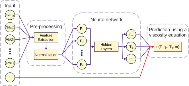
Figure 1 shows a flowchart of the machine learning pipeline used here. The arrows indicate the flow of information that starts from the input data (composition and temperature of the liquid) and ends with the prediction of viscosity by the viscosity equation.

The neural network in the pipeline is a predictor of the viscosity parameters, namely $\eta_{\infty}$, $T_{g}$, and $m$. These parameters, along with temperature, serve as inputs for the viscosity equation, which makes the final prediction. One advantage of this gray-box approach—in contrast with a black-box approach—is that the viscosity parameters can be predicted individually. Hence, the same trained model predicts not only the temperature-dependence of viscosity but also the liquid’s fragility index and its glass transition temperature.

The machine learning pipeline shown in Fig. 1 has many hyperparameters, such as the number of hidden layers in the NN and their size, for example. The methodology for finding a good set of hyperparameters is discussed in detail in Section 2.4. However, some hyperparameters were fixed from the beginning as design choices. The viscosity equation used in the pipeline is one of these fixed hyperparameters; it was the MYEGA equation. The backpropagation loss function is another fixed hyperparameter; it was chosen as the mean squared error (MSE) because it is a suitable loss function to solve regression problems.

2.3 Feature extraction and selection

Table 1: Chemical properties considered in this work. ^† based on DFT volume of the OQMD ground state [31, 32]. ^* computed in DFT simulation of $T=$ $0\text{\,}\mathrm{K}$ ground state.

Atomic number

Atomic weight

Atomic volume

Atomic radius [33]

Atomic radius [34, 35]

Boiling point

Melting point

C6 coefficient [36]

Covalent radius [37]

Single-bond covalent radius [38]

Double-bond covalent radius [39]

Density

Dipole polarizability

Effective nuclear charge

Electron affinity

Energy to remove the first electron

Electronegativity in the Gosh scale [40]

Electronegativity in the Pauling scale

Electronegativity in the Sanderson scale

Electronegativity in the Martynov-Batsanov scale

Fusion enthalpy

Glawe’s number [41]

Mendeleev’s number

Pettifor’s number [42]

Heat of formation

Lattice constant

BCC lattice parameter†

FCC lattice parameter†

Mass number of the most abundant isotope

Maximum ionization energy

Number of electrons

Number of neutrons

Number of protons

Number of valence electrons [43]

Number of valence electrons [44]

Number of unfilled valence orbitals

Number of unfilled s valence orbitals

Number of unfilled p valence orbitals

Number of unfilled d valence orbitals

Number of unfilled f valence orbitals

Number of filled s valence orbitals

Number of filled p valence orbitals

Number of filled d valence orbitals

Number of filled f valence orbitals

Number of oxidation states

Bandgap energy*

Energy per atom*

Magnetic moment*

Volume per atom*

Space group*

Radii of element in metallic glass structure

Van der Walls radius [45]

Van der Walls radius [46]

Van der Walls radius [47]

Van der Walls radius [48]

Van der Walls radius [49]

In the chemical composition domain, the features of a liquid are represented by a vector with the atomic mole fraction of its constituents. To convert these features to the chemical property domain, one must choose a chemical property and an aggregator function. An example is to choose the atomic weight as a property and compute the “mean atomic weight,” which is a feature of the liquid. By choosing different chemical properties and aggregator functions, one can “extract” new features from the liquid in the chemical property domain. This procedure is called feature extraction or feature engineering [50].

The mathematical procedure for this process starts by creating the vector $\boldsymbol{C}=\left[x_{1},x_{2},\ldots,x_{n}\right]$ of the atomic mole fractions of the chemical elements $e_{1}$, $e_{2}$, …, $e_{n}$ that make a certain liquid. Let $\boldsymbol{S}=\left[s_{1},s_{2},\ldots,s_{n}\right]$ be the vector of a certain chemical property $s_{i}$ of the chemical element $e_{i}$ (the atomic weight, for example). We compute the property vectors $\boldsymbol{W}$ (weighted) and $\boldsymbol{A}$ (absolute) as

$$\boldsymbol{W}=\boldsymbol{C}\boldsymbol{S}^{T},$$ (3)

and

$$\boldsymbol{A}=\left\lceil\boldsymbol{C}\right\rceil\boldsymbol{S}^{T}.$$ (4)

Note that the ceil function is applied element-wise in vector $\boldsymbol{C}$ in Eq. (4).

Finally, by applying an aggregator function to the items of the vectors $\boldsymbol{W}$ or $\boldsymbol{A}$, one obtains a particular chemical feature of the liquid. The aggregator functions used in this work are summation, mean, standard deviation, minimum, and maximum. Many features can be extracted following this procedure. This work considered all the chemical properties shown in Table 2.3, which are available in the Python modules mendeleev [43] and matminer [44].

A total of 601 chemical property features were extracted using this procedure. A feature selection routine to eliminate features with high collinearity and low variance was performed as follows:

1. Let $l$ be the set of all chemical property features;

2. Compute the variance inflation factor (VIF) [51] of all the features in $l$;

3. Let $v$ be the maximum value of all the computed VIFs;

4. If $v>10$, then the feature associated with this VIF is removed from $l$ because its collinearity is too high. If a feature was removed in this step, return to step 2;

5. If $v\leq 10$, then the standard deviation is computed for all remaining features. Those features with a standard deviation of less than ${10}^{-3}$ are removed from $l$ because they have too low variance;

6. The remaining features in $l$ are the features used in this work.

Only chemical property features were extracted in this work. However, in the framework proposed by Adam and Gibbs [52] (which is the basis for the MYEGA equation), viscosity depends on the size of the cooperative rearranging regions, which are related to the atomic structure of the liquid. Therefore, a predictor of viscosity that uses only chemical features is unlikely to generalize all the intricacies of viscous flow. Structural features, however, are outside of the scope of this work. To avoid data leakage [53], feature selection was performed using only data not reserved in the test dataset.

2.4 Hyperparameter tuning

The prediction power and the generalization power of a neural network are highly dependent on its hyperparameters (HP), such as the number of neurons, number of hidden layers, and activation function. Determining a good set of HP for a new problem is not trivial. Thus, before settling for the final network architecture, it is vital to test many sets of HP, a process called hyperparameter tuning.

HP tuning was performed in a sequence of three experiments, starting with a random search, then a Bayesian search, and finally, a 10-fold cross-validation. These experiments were done in series, with the second and third using knowledge obtained in the previous experiments.

The first experiment was the test of 500 different HP sets, randomly drawn from the search space shown in Table 2. For each HP set that was drawn, a neural network was built and trained. Only the 762 liquids that were not part of the test dataset were used in this experiment. The training and validation datasets were the same for all NNs in this experiment and consisted of the data points of 686 and 76 randomly chosen liquids, respectively (90–10 split). This split strategy was chosen with extrapolation (instead of interpolation) performance in mind: all the data points in the validation dataset are from liquids with different chemical composition than those in the training dataset. The training of the NNs was terminated if their performance was not good enough when compared with the finished trials (using an Asynchronous Successive Halving Algorithm, ASHA [54]), or until no improvement in the prediction of the validation dataset was observed after a particular number of epochs determined by the “patience” hyperparameter. The average MSE loss of the validation dataset was recorded for all HP sets.

Tabela 2: Hyperparameters search space for experiments 1 and 2, and selected HP set after cross-validation. The functions Tanh and ReLU are the hyperbolic tangent and the rectifier linear unit. SGD is the stochastic gradient descent [55, 56]. Adam [57] and AdamW [57, 58] are stochastic gradient descent methods based on an adaptive estimation of first-order and second-order moments, the latter having a weight decay coefficient.

Hyperparameter	1st Experiment	2nd Experiment	Selected
Number of hidden layers	{1,2,3}		2
Training batch size	{2, 4, 8, 16, 32, 64, 128}		64
Patience (integer)	[5, 20]	[5, 25]	9
Optimizer	{SGD, Adam, AdamW}		AdamW
Optimizer learning rate	[${10}^{-5}$, ${10}^{-1}$]		$1.16\text{\times}{10}^{-3}$
SGD momentum	[0, 1]		—
1st hidden layer
Size (integer)	[16, 256]	[16, 512]	192
Dropout (%)	[0, 50]		7.94
Use batch normalization	{Yes, No}		No
Activation function	{ReLU, Tanh}		ReLU
2nd hidden layer
Size (integer)	[16, 256]		48
Dropout (%)	[0, 50]		5.37
Use batch normalization	{Yes, No}		No
Activation function	{ReLU, Tanh}		Tanh
3rd hidden layer
Size (integer)	[16, 256]		—
Dropout (%)	[0, 50]		—
Use batch normalization	{Yes, No}		—
Activation function	{ReLU, Tanh}		—

The second experiment was the test of 300 different HP sets, drawn from the search space shown in Table 2. This search space is almost identical to that of the first experiment, but allowing for bigger size of the first hidden layer and for higher values of patience—a choice made after observing that the top 100 HP sets from the previous experiment were too close to the upper bound limit of these two hyperparameters. All the other characteristics of the second experiment are the same as the first, except that the HP sets were not drawn randomly but instead guided by a Tree-structured Parzen Estimator algorithm [59]. The first 20 HP sets, however, were the 20 HP sets that performed the best in the first experiment, that is, those with the lowest average MSE loss of the validation dataset.

The third and final experiment was a 10-fold cross-validation for each of the 10 HP sets with the lowest average MSE validation loss among all the 700 HP sets tested in this work. A 10-fold cross-validation experiment consists of splitting the data into 10 different sets called folds. Each of these folds is selected once to be the validation dataset, with the remaining folds making the training dataset. A NN is trained for each of these different training and validation datasets. The HP set with the lowest average of the validation losses in this analysis was selected as the final architecture for the neural network. For all three experiments, the validation dataset always contained only liquids that were not present in the training dataset.

All experiments were coded in the Python programming language, and the NN were trained using a personal computer with an 8-core CPU and 16 GB of RAM. The neural networks were built using the PyTorch-Lightning module [60], a high-level interface for PyTorch [61]. Data management was performed with the pandas module [62]. Hyperparameter tuning was performed using tune [63] (first and second experiments) and hyperopt [64] (second experiment). Cross-validation and data splitting was performed using sklearn [65].

3 Results and discussion

3.1 Data analysis

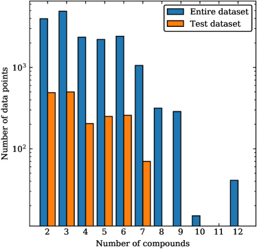
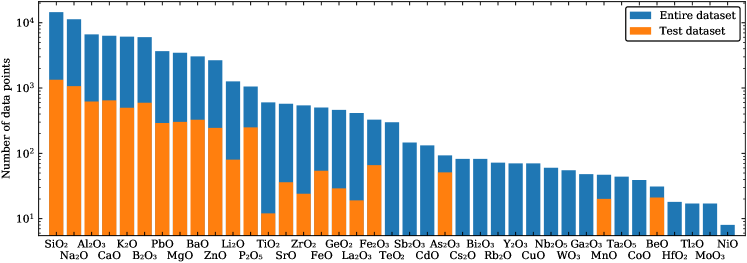
Figure 2 has three plots with information on the entire viscosity dataset used in this work, together with the test dataset. The plot in Fig. 1a shows the histogram of the number of different compounds of the liquids, the overall maximum is 12, and the maximum of the test dataset is 7. As expected, the number of data points has an inverse correlation with the number of compounds because simple liquids are more studied than complex ones.

(a)

(b)

(c)

Figura 2: Data analysis of the entire dataset and the test dataset. (a) Histogram of the number of compounds in the liquid. (b) Histogram of the viscosity values. (c) Histogram for each compound, the orange regions represent the fraction selected for the test dataset.

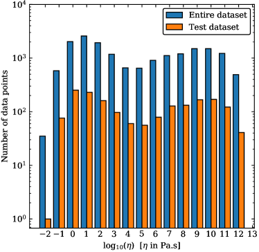
The histogram in Fig. 1b shows a bimodal distribution of the viscosity values, with a local minimum around the center at ${10}^{5}\text{\,}\mathrm{P}\mathrm{a}\,\mathrm{s}$. Measuring viscosity in this central region is challenging: the liquid has enough kinetic enengy and thermodynamic driving force to crystallize, which often happens too fast and forcibly ends the viscometry experiment.

Finally, the histogram in Fig. 1c shows the number of data points per compound for the entire dataset, with the fraction used for the test dataset marked in orange. Most liquids are made with SiO2, Na2O, and Al2O3, which are common compounds used in the glass industry. Not all compounds are part of the test dataset because of the way it was produced. As discussed in Section 2.1, the test dataset contains 85 randomly selected liquids from the entire dataset, not a certain number of randomly selected data points from this dataset.

3.2 Feature extraction and selection

The feature extraction procedure generated a total of 601 chemical property features extracted from the chemical composition. From this total, 35 features shown in Table 3.2 were selected. The feature selection procedure considered the collinearity and variance of the 601 initial features, not their relationship with viscosity. Finding which of these features are more or less relevant to model viscosity was a task left to the NN.

Tabela 3: Type, aggregator function, and chemical property of the 35 selected features. “W” stands for weighed (see Eq. (3)) and “A” stands for absolute (see Eq. (4)). SD is the standard deviation.

Type

Aggregator

Chemical property

W& Maximum Atomic radius W Maximum Atomic volume W Maximum Bandgap energy W Maximum C₆ coefficient [36] W Maximum Number of filled d valence orbitals W Maximum Number of unfilled s orbitals W Maximum Number of unfilled d orbitals W Maximum Number of oxidation states W Maximum Number of valence electrons [44] W Maximum Space group W Maximum Volume per atom W Minimum Fusion enthalpy W Minimum C₆ coefficient [36] W Minimum Maximum ionization energy W Minimum Number of valence electrons [44] W Minimum Number of valence electrons [43] W Minimum Space group W Mean Magnetic moment W SD Radii of element in metallic glass structure A SD Atomic radius [34, 35] A SD C₆ coefficient [36] A SD Effective nuclear charge A SD Electron affinity A SD Energy per atom A SD Fusion enthalpy A SD Lattice constant A SD Magnetic moment A SD Mendeleev’s number A SD Number of filled f valence orbitals A SD Number of unfilled p valence orbitals A SD Number of unfilled d valence orbitals A SD Number of oxidation states A SD Number of valence electrons [43] A SD Van der Walls radius [46] A SD Van der Walls radius [48]

3.3 Building and training the model

The selected neural network architecture after HP tuning is shown in the last column of Table 2. It is a deep network with two hidden layers, the first layer with 192 neurons and the second layer with 48 neurons, both having dropout [66] and not having batch normalization [67]. Interestingly, this network has mixed activation functions, with ReLU for the first layer and Tanh for the second. The machine learning pipeline containing this network will be called ViscNet from now on.

Two notable differences between ViscNet and the NN reported by Tandia et al. [13] is the number of layers and their size (number of neurons). Both hyperparameters are higher in this work; although the final architecture was not disclosed by Tandia et al., a single-layer with about 10 neurons was strongly suggested. Nonetheless, the two models differ in scope, considering that the NN reported by Tandia et al. is focused on particular liquid compositions (9 different chemical compounds). A smaller scope explains the difference in complexity.

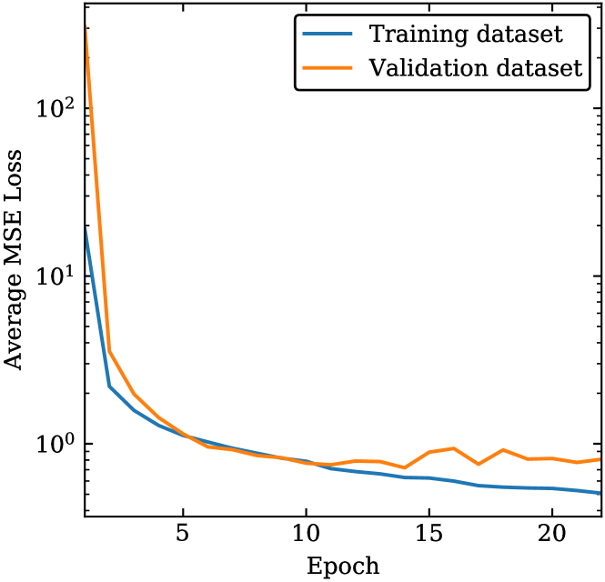
Interestingly, the activation function used in by Tandia et al. [13] (single-layer) and of the second (final) layer of this work is the same, a hyperbolic tangent. Finally, Fig. 3 shows the learning curve of the ViscNet neural network; no clear sign of overfitting is present in this figure.

Figura 3: Learning curve of the ViscNet neural network. An epoch is when all the training data passes through the network during the training phase.

3.4 Performance of the model

There are many ways to assess the performance of predictive models; metrics such as the coefficient of determination ($R^{2}$), the root mean squared error (RMSE), the mean absolute error (MAE), and the median absolute error (MedAE) give a holistic view on the performance of regressors. Table 4 shows these metrics of ViscNet for the cross-validation experiment and the prediction of the training, validation, and testing datasets. More information on these metrics can be found in the Appendix. As expected, the training dataset metrics are better than those of the validation dataset, which in turn are better than those of the test dataset. These differences reflect the influence that these datasets have in the training of the model: the training dataset was used to change the weights and bias of the network, the validation dataset was used to stop training before it starts overfitting, and the test dataset had no influence whatsoever in the training process. The cross-validation experiment metrics are comparable to the metrics of the validation dataset, as expected.

Tabela 4: Metrics of ViscNet for the cross-validation experiment and the training, validation, and test datasets. The symbol $\uparrow$ indicates that the higher the metric, the better, whereas the symbol $\downarrow$ indicates the opposite. The cross-validation column values are the mean and standard deviation of the metrics for the 10 folds.

Metric	Training	Validation	Cross-val.	Test
$R^{2}$ ($\uparrow$)	0.99	0.98	$0.980(5)$	0.97
RMSE ($\downarrow$)	0.58	0.88	$0.9(1)$	1.1
MAE ($\downarrow$)	0.42	0.64	$0.60(8)$	0.78
MedAE ($\downarrow$)	0.33	0.46	$0.38(6)$	0.53

The performance metrics obtained here were not as good as those reported by Tandia et al. [13]. They achieved an impressive $R^{2}$ value of 0.9999 and RMSE of 0.04 for the best architecture on their validation dataset. Possible explanations for this difference are related to the quality of the data, the number of chemical compounds used for training, and the strategy to split the dataset. Tandia et al. used a proprietary dataset owned by Corning Inc. that presumably has much less variance than the dataset collected from SciGlass. The number of chemical compounds used for training was 9 in Ref. [13] and 39 in this work; it is more difficult for a model to generalize in a diverse chemical domain. Finally, it is not stated if the dataset spliting strategy used in Ref. [13] is similar to the one used in this work (validation and test dataset are made of liquids that are not present in the training dataset) or if it is the commonly used random splitting; the expectation is that the latter would yield better metrics as interpolation is easier than extrapolation.

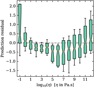
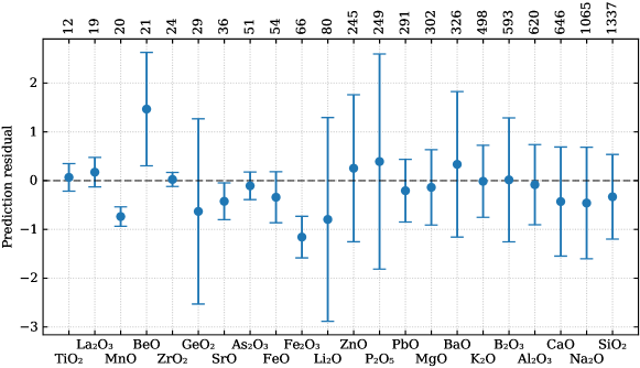
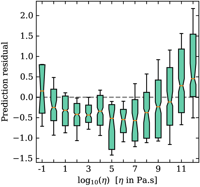
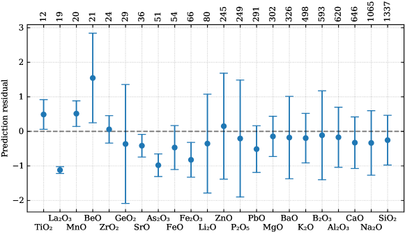
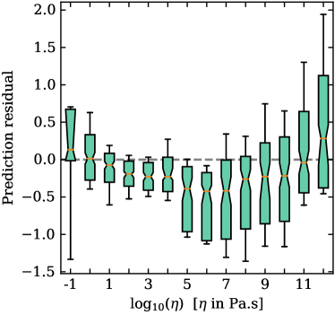
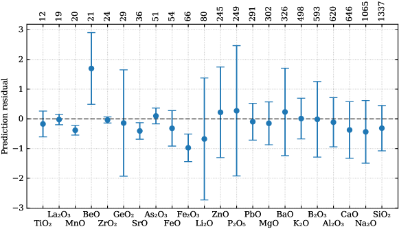
Another strategy to assess the performance of ViscNet is by looking into the prediction residuals. Figures 4 and 5 show the prediction residual versus the viscosity range and the chemical compound in the liquid, respectively. Both plots show only predictions for the test dataset, as these predictions suggest how well the model can predict data that it has never seen, thus helping assess the generalization capabilities of the model.

Figure 4 shows that the prediction’s uncertainty is higher for higher values of viscosity. However, the median prediction residual is in the range of $-0.5$ and 0.5, which is expected as the MedAE for the test dataset is about 0.5. Figure 5 shows that some compounds such as GeO2, LiO2, ZnO, P2O5, B2O3, BeO, and BaO have a standard deviation of the prediction residual greater than one. Care should be taken when using ViscNet to predict liquids having these compounds.

Figura 4: Boxplot of the prediction residual versus the reported value of viscosity for the test dataset. The boxes are bound by $25\text{\,}\mathrm{\char 37\relax}$ and $75\text{\,}\mathrm{\char 37\relax}$ percentiles, and the error caps represent $67\text{\,}\mathrm{\char 37\relax}$ of the data. The median is shown as a horizontal orange line, and the notch of the median represents its $95\text{\,}\mathrm{\char 37\relax}$ confidence interval.

Figura 5: Mean and standard deviation of the prediction residual versus the chemical compound for the test dataset. The top $x$-axis shows the number of data points in the test dataset that have the respective compound; it is organized in crescent order from left to right.

All the liquids in the test dataset have compositions that were not present in the datasets used for training and validating the model. This splitting strategy was a design choice to promote better extrapolation instead of better interpolation of viscosity. A question that arises is if the prediction accuracy is related to how distant the composition is to the domain of training. The distance used was the Canberra distance between the composition vector of the liquid and its closest neighbor in the training and validation domain. The Canberra distance is a weighed $L_{1}$ distance; $L_{2}$ distances (such as Euclidean) are not recommended for problems with more than three dimensions [68]. Figure 6 shows that most liquids in the test dataset have an RMSE close to 0.5, but as the distance increases, so do the chances of having a higher value of RMSE.

Figura 6: RMSE of prediction of the liquids in the test dataset versus their distance from the training and validation domain (see text). Each point represents a different liquid. The dashed gray line shows RMSE = 0.5.

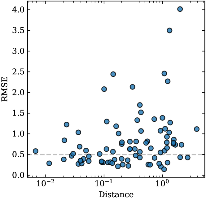
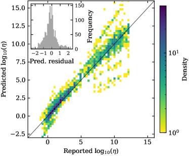
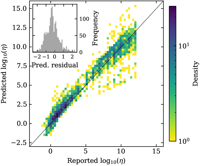
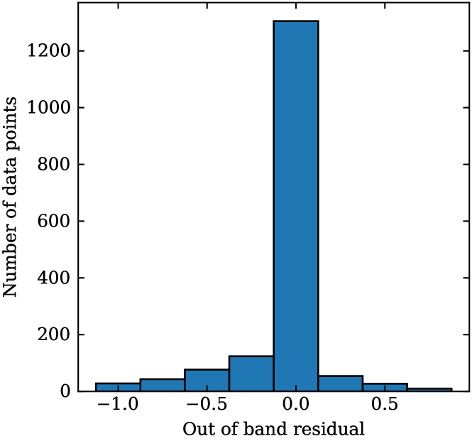
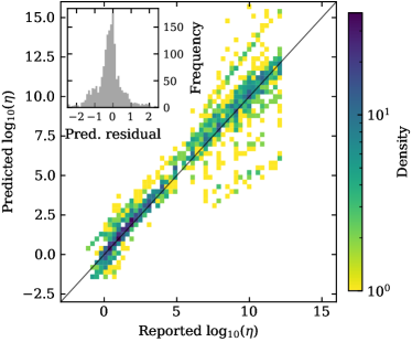
Figure 7 shows a 2D histogram with the correlation between the predicted and reported viscosity values of the test dataset. Most of the data points are close to the identity line, but a noticeable spread is present, especially in the region of higher viscosity (as already suggested by Fig. 4). The inset of this plot shows a histogram of the prediction residuals. The model has a small bias towards predicting higher values of viscosity than those reported.

Figura 7: 2D histogram of predicted versus reported values of $\log_{10}\left(\eta\right)$ for the test dataset. Each square has a corner of 0.3, and the continuous black line is the identity line. The inset is the histogram of the prediction residuals.

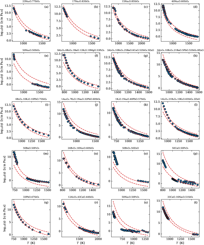
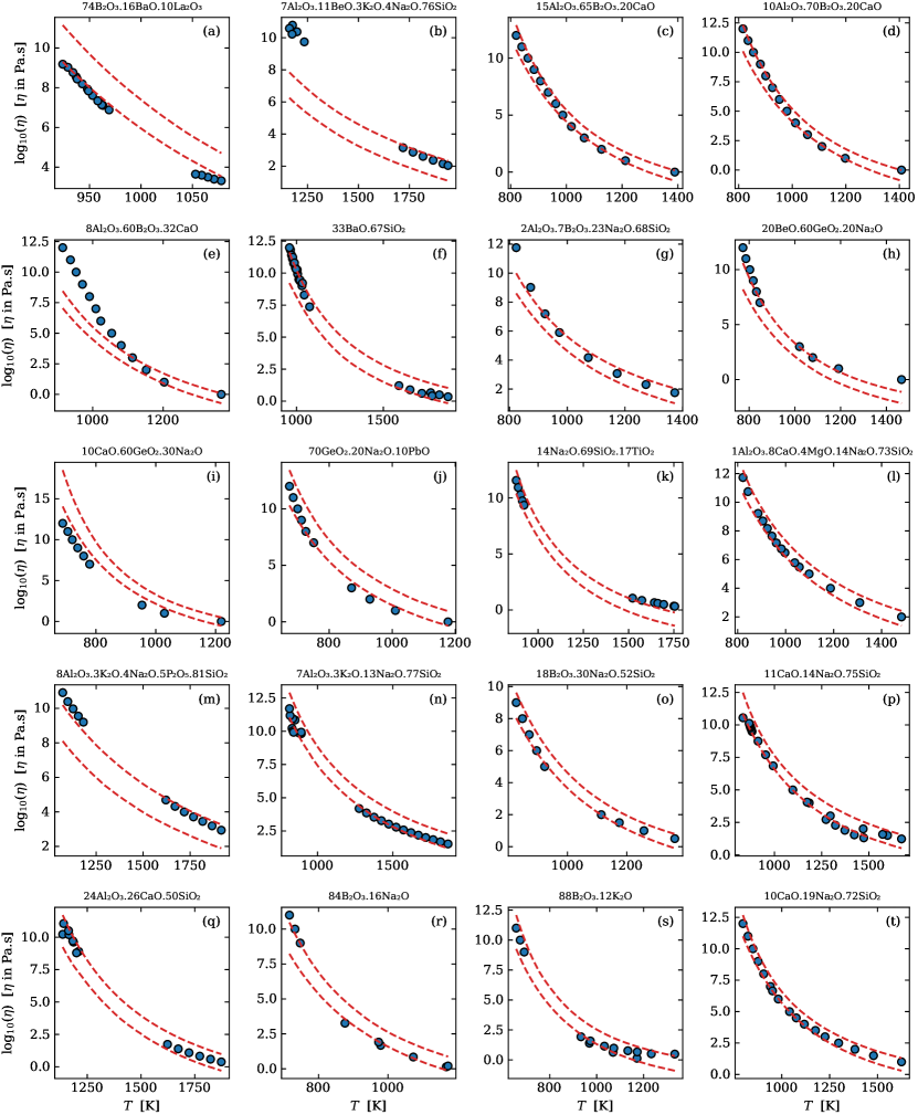
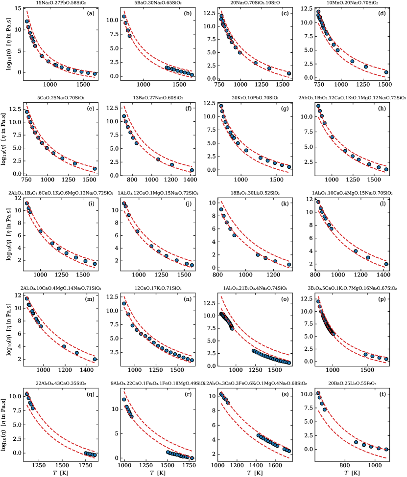
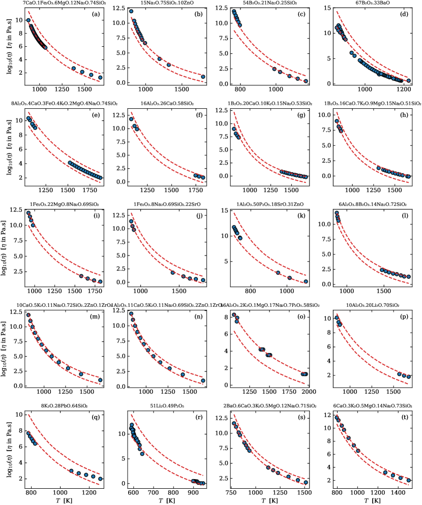
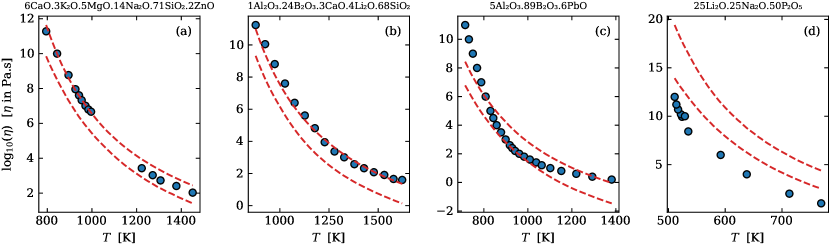
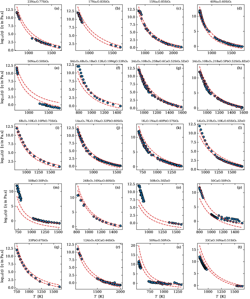
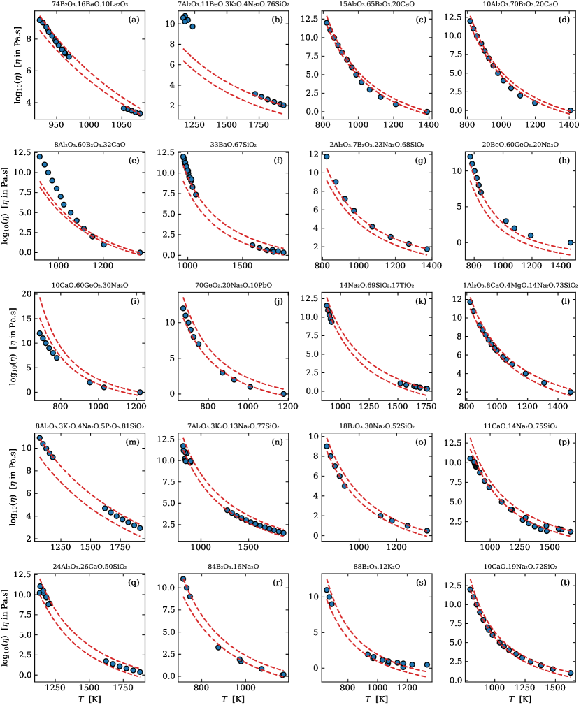
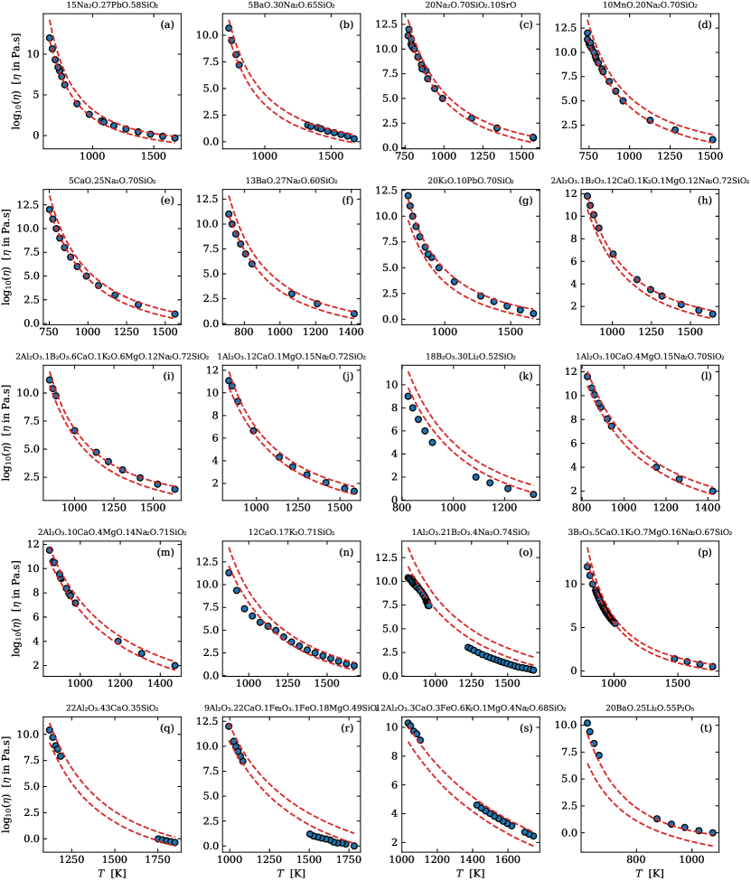
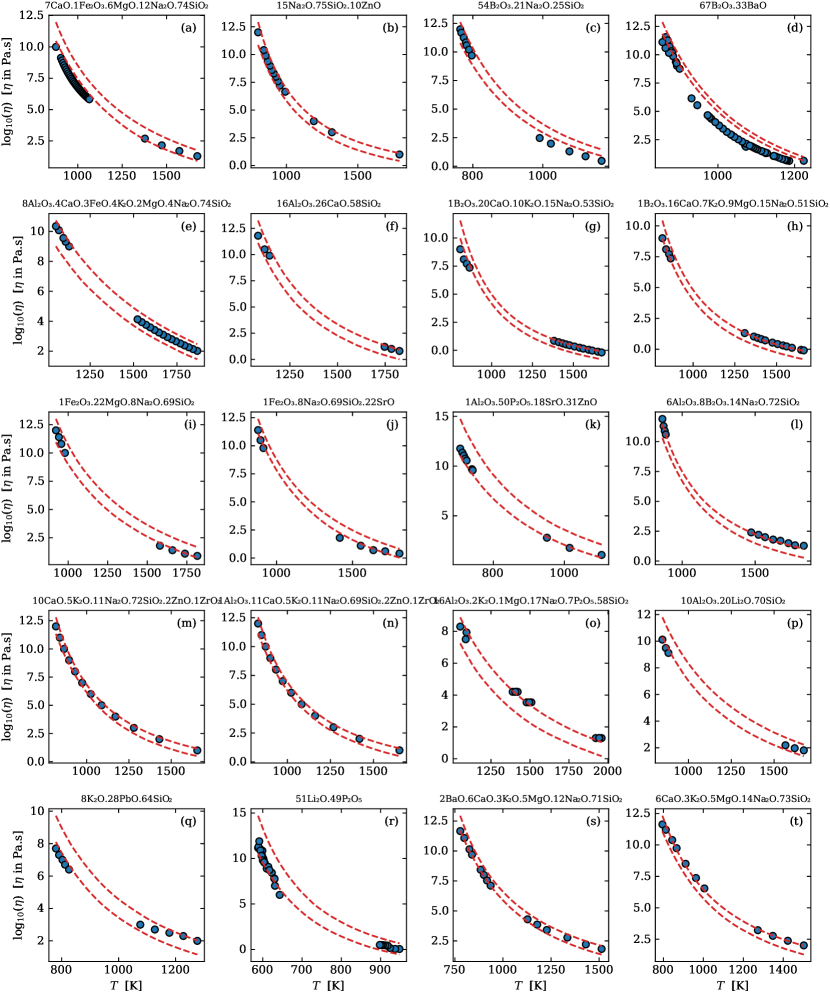
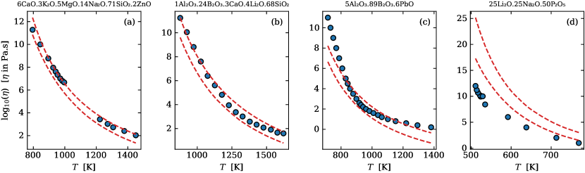
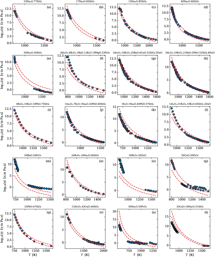
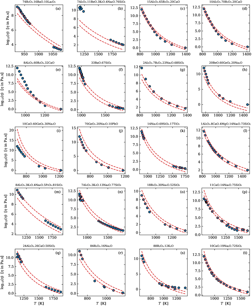
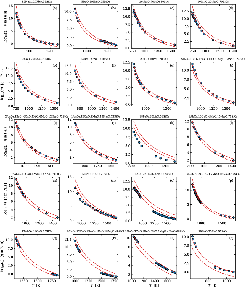
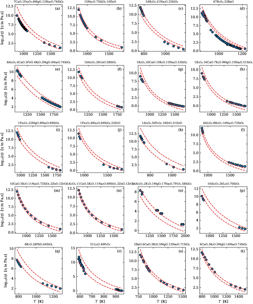
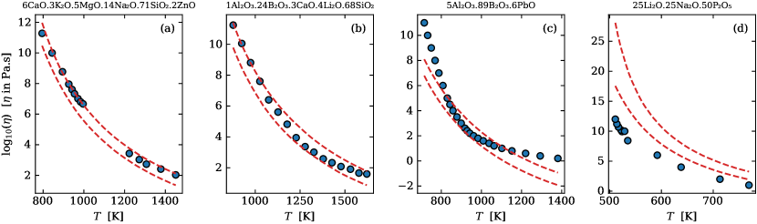
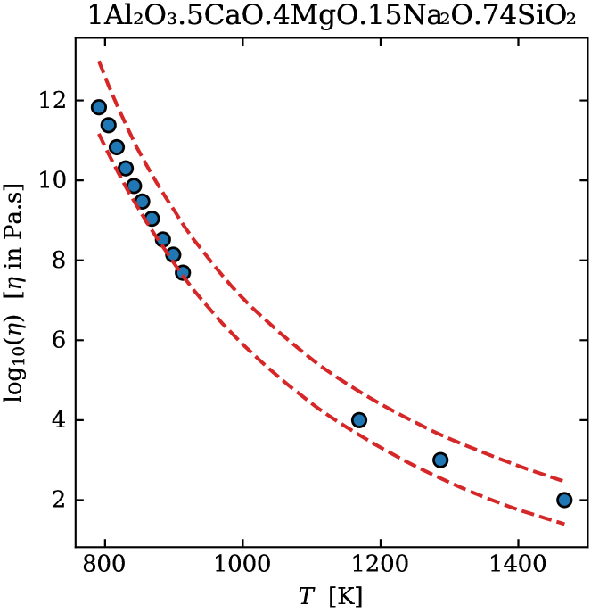
The final analysis of the ViscNet performance consists of looking at the data points and the model prediction for all the liquids in the test dataset. Figure 8 shows this analysis for one of the liquids; individual plots for all the other 84 liquids are shown in the Appendix. The uncertainty of prediction represents a confidence interval of $95\text{\,}\mathrm{\char 37\relax}$ and was computed by Monte Carlo dropout [69] with $1000$ random samples. For many liquids in the test dataset, the uncertainty bands contain the experimental data or predict the general trend of viscosity correctly. Figure 9 shows that $1200$ data points of the test dataset (about $70\text{\,}\mathrm{\char 37\relax}$) are within the prediction bands of the model. There are problematic compositions, as expected, where neither the magnitude nor temperature-dependence of viscosity was adequately predicted. As already discussed, predicting the viscosity for a liquid too far from the training and validation domain increases the chances of a wrong prediction. A (labor intense) solution is to collect more data to expand the training domain; another solution is to train the model with structural features in addition to chemical features.

Figura 8: Base-10 logarithm of viscosity versus temperature for Al2O3.5CaO.4MgO.15Na2O.74SiO2, one of the liquids in the test dataset. The blue circles are experimental data, and the dashed red lines are the model uncertainty bands with a confidence interval of $95\text{\,}\mathrm{\char 37\relax}$.

Figura 9: Histogram of out of band residual values of the test dataset prediction. The out of band residual is zero if the data point is within the prediction bands or the difference between the reported viscosity value and the closest uncertainty band otherwise (in base-10 logarithm scale).

3.5 Parameters of viscosity

As already mentioned, one advantage of the gray-box approach, in contrast with the black-box approach, is the direct access to the parameters of the viscosity model. Figure 10 leverages this advantage by showing the prediction of the glass transition temperature and the fragility index for the ternary system SiO2-Na2O-Al2O3, one of the base systems currently used for developing scratch-resistant display screens. The predictions of both properties are contained only in the region that the composition vector has a distance of 0.5 or less to its closest neighbor in the training and validation domain. As shown in the previous section, going too far away from this domain increases the chance of a wrong prediction.

(a)

(b)

Figura 10: Ternary plot of (a) $T_{g}$ and (b) fragility index for the system SiO2-Na2O-Al2O3 predicted by ViscNet. For better visualization, $T_{g}$ values were rounded to the closest multiple of 50 and fragility index values to the closest multiple of 2. Only data with a distance of 0.5 or less of the closest neighbor in the training and validation domain are shown in the plots (see Fig. 6 and related discussion). Out of domain (OoD) region is shown in white.

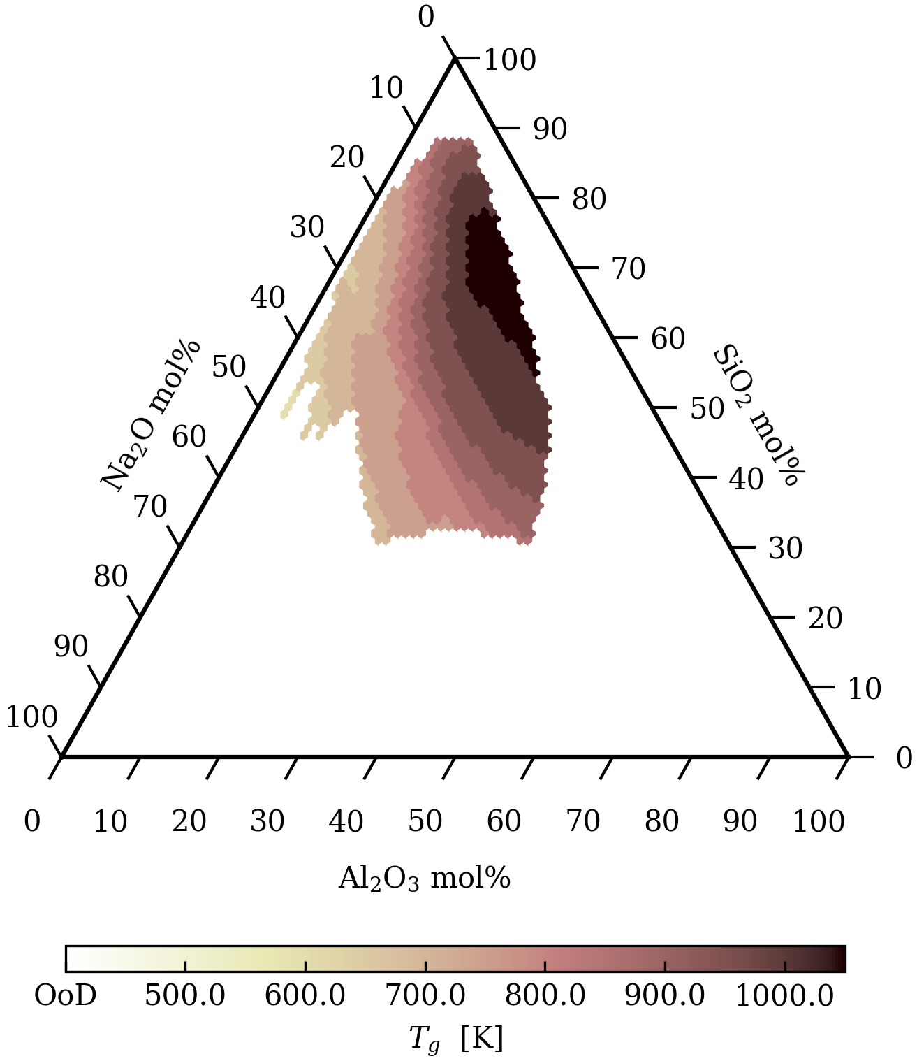
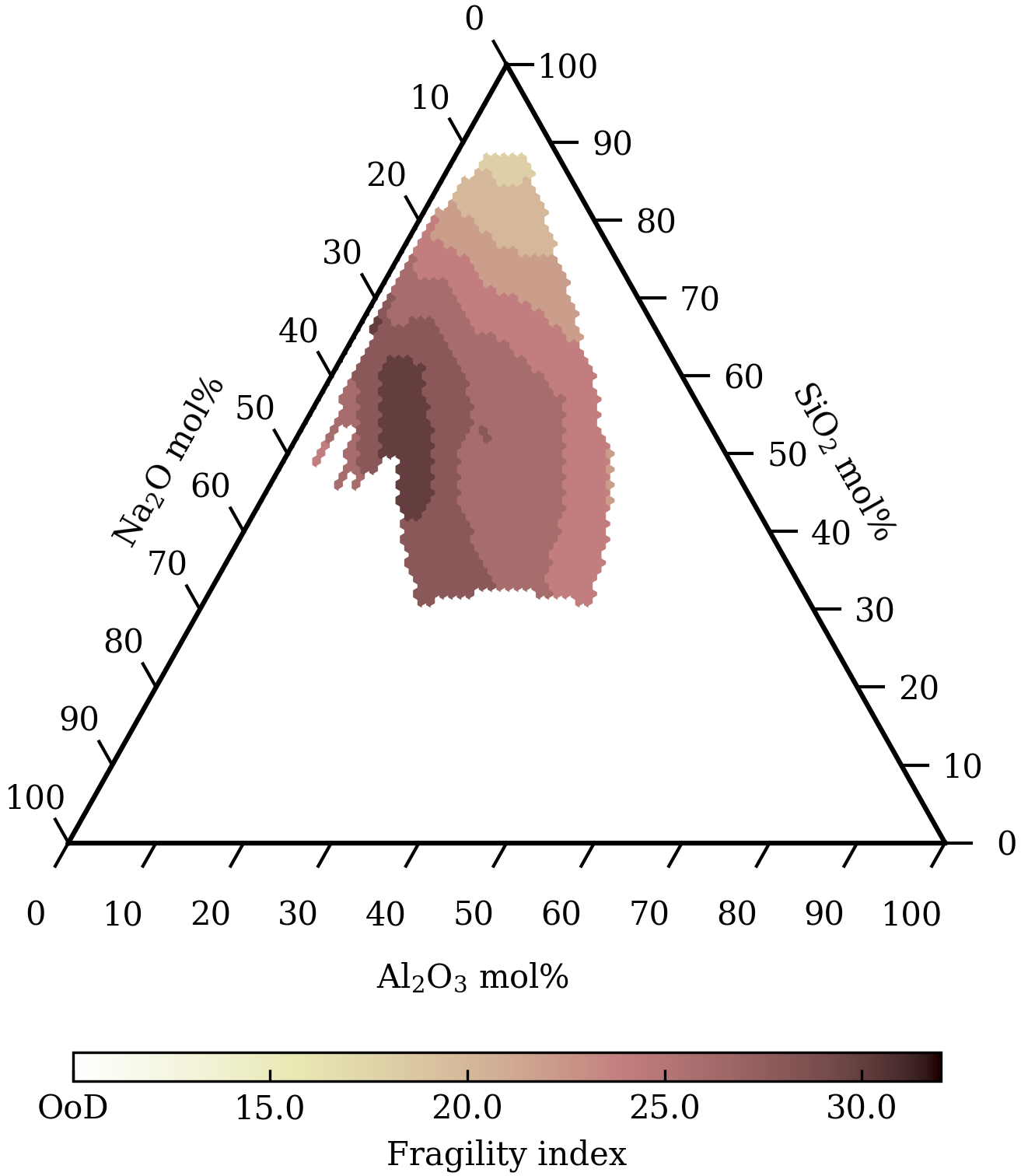
The plots in Fig. 10 show that the glass transition temperature decreases significantly with the addition of Na2O but changes at a much lower rate with the addition of Al2O3. While this is well known in the glass community (Na2O is a modifier and Al2O3 is an intermediate compound), it is interesting to see that the model could capture this behavior from data. The fragility index follows a similar trend, but with $m$ increasing instead of decreasing with the addition of Na2O and Al2O3.

3.6 Transfer learning

As already mentioned, some hyperparameters were fixed from the very beginning, during the machine learning pipeline design. The viscosity model and the backpropagation loss function are two examples.

Another three-parameter viscosity model is the VFT empirical equation (Eq. (5)) [70, 71, 72], which has historical significance and is still often used in scientific research. It is possible to build a machine learning pipeline similar to that shown in Fig. 1, but with the VFT equation instead of the MYEGA equation, and use the weights and bias of ViscNet as a starting point for the new model; this process is called transfer learning. The resulting model following this strategy will be called ViscNet-VFT.

$$\log_{10}\left(\eta\left(T,\eta_{\infty},T_{g},m\right)\right)=\log_{10}\left(\eta_{\infty}\right)\\ +\frac{\left(12-\log_{10}\left(\eta_{\infty}\right)\right)^{2}}{m\left(T/T_{g}-1\right)+\left(12-\log_{10}\left(\eta_{\infty}\right)\right)}$$ (5)

The same procedure can be used to explore different backpropagation loss functions. The loss function of the original pipeline was the MSE, which is sensitive to outliers. By using transfer learning, we can change this loss function to one that is robust against outliers, such as the Huber loss [73]. The resulting model following this strategy will be called ViscNet-Huber.

One advantage of using transfer learning is that it is significantly faster than developing a model bottom-up. The HP tuning routine for ViscNet took about a day and a half of computing time while training both new models using transfer learning took only a few minutes.

The prediction power of ViscNet-VFT is comparable to that of ViscNet. This result is expected as the MYEGA and VFT equations both yield similar results in the temperature range where experimental data is available. They significantly differ, however, if the model is extrapolated to regions where the viscosity is higher than ${10}^{12}\text{\,}\mathrm{P}\mathrm{a}\,\mathrm{s}$.

Any other three-parameter viscosity model that can be formulated in function of $\eta_{\infty}$, $T_{g}$, and $m$ (such as the AM equation [74], for example) can also be used to create other models via transfer learning, similarly to what was performed with the VFT equation. However, the expectation is that no significant differences in prediction power will be observed in the temperature range where experimental data are available, as was the case with VFT.

Using transfer learning to change the loss function had an interesting consequence: ViscNet-Huber is better at predicting high-temperature viscosity than ViscNet (see Fig. 10a). This temperature region is particularly important for processing glasses via melt and quench, which is the most used route to process commercial glasses.

Figure 11 shows some results on the prediction power of ViscNet-Huber. Additional plots are available in the Appendix for the interested reader. Apparently, this work is the first to use transfer learning in the context of glass-forming liquids.

(a)

(b)

(c)

Figura 11: Results of the ViscNet-Huber model for the test dataset: (a) boxplot of the prediction residual versus the reported value of viscosity; (b) 2D histogram of predicted versus reported values of $\log_{10}\left(\eta\right)$; and (c) mean and standard deviation of the prediction residual versus the chemical compound. See Section 3.4 for information on how these plots were made.

3.7 Reproducibility and data availability

This work was entirely performed using open-source software and the SciGlass database, which has a permissive license. Code containing all the necessary functions to load the data and train the machine learning pipelines discussed here is publicly available on GitHub (https://github.com/drcassar/viscnet) and Zenodo [75], licensed as free software under the GPL3. This code leverages deterministic routines for training the NNs provided by the PyTorch-Lightning module; thus interested readers can reproduce the exact models reported here. Pretrained networks for ViscNet, ViscNet-Huber, and ViscNet-VFT are also available in the repository.

Due to the free and open-source nature of the data and the code, anyone can extend the procedures presented here to better meet their needs, for example, including new features for training the models or training the models with different datasets.

4 Conclusion

This work aimed to build a machine learning pipeline to predict the temperature-dependence of the viscosity of oxide liquids, inspired by a recent gray-box neural network developed by Tandia et al. [13], who embedded a physical model in the pipeline. This work introduced a pre-processing unit with a chemical feature extractor, which changes the feature domain from chemical composition to chemical properties.

The predictive model was focused on extrapolation, and it was able to predict the viscosity of the 85 liquids in the test dataset with an $R^{2}$ of 0.97. About $70\text{\,}\mathrm{\char 37\relax}$ of the data points in the test dataset where within the uncertainty bands of the model’s prediction. However, the chances of a wrong prediction increases with the distance to the closest neighbor in the training and validation datasets.

The performance and speed of the predictive models can be exploited to guide the development of new glasses. The viscosity prediction can help in selecting compositions with a particular viscosity behavior or determining process variables. The fragility index and glass transition temperature predictions can help in selecting compositions with desired properties for specific applications.

All code used in this work was built with reproducibility in mind, using open-source Python modules. Both data and code are available for anyone interested, at no cost, and with a permissive license: the hope is that this free and open framework for property prediction could be used and improved by the community to accelerate the development of new materials.

Acknowledgments

The author is thankful for the São Paulo State Research Foundation support (FAPESP grant number 2017/12491-0) as well as for the Nippon Sheet Glass Foundation overseas research grant. The author also thanks John Mauro, Adama Tandia, Bruno Rodrigues, and Collin Wilkinson for insightful comments and suggestions; and Carolina Zanelli for text revision.

Data availability statement

The viscosity data used in this work comes from the SciGlass database. This database is available under an ODC Open Database License (ODbL) at https://github.com/epam/SciGlass. See Section 3.7 for more information on reproducing this research.

Competing interest statement

The author declares no competing financial or non-financial interests.

Appendix

Apêndice A z-score

In the pre-processing unit of the machine learning pipeline, a normalization step computes the z-score $z_{i}$ of each feature that will be fed to the NN. This process (Eq. (6)) is performed for each feature $f_{i}$ by subtracting the mean value of this feature ($\mu$) and scaling the data to unit variance by dividing by the standard deviation of this feature ($s_{d}$).

$$z_{i}=\frac{f_{i}-\mu}{s_{d}}$$ (6)

Apêndice B Evaluation metrics

Four metrics were computed in Section 3.4 and are discussed here.

The coefficient of determination, $R^{2}$, has various definitions. Here it is used to test the relationship between the predicted and the reported base-10 logarithm of viscosity ($\hat{y}$ and $y$, respectively). The ideal relationship is a linear model with no intercept, for which the $R^{2}$ can be computed via Eq. (7). The value of $R^{2}$ is dimensionless and between zero and one, indicating, respectively, no correlation and a perfect correlation between predicted and reported viscosity values.

$$R^{2}=1-\frac{\sum_{i}^{n}\left(y_{i}-\hat{y_{i}}\right)^{2}}{\sum_{i}^{n}y_{i}^{2}}$$ (7)

The root mean square error, RMSE, is a measure of the difference between $y$ and $\hat{y}$. It is the square root of the mean square error, as can be seen in Eq. (8), and it has the advantage of being in the same unit as $y$. The lower the RMSE, the better.

$$\mathrm{RMSE}=\sqrt{\frac{1}{n}\sum_{i}^{n}\left(y_{i}-\hat{y}_{i}\right)^{2}}$$ (8)

The mean absolute error MAE is the average of the absolute errors. It is also a measure of the difference between $y$ and $\hat{y}$, but differently from RMSE, each error contributes equally, and the residuals are not squared. This metric has the same unit as $y$ and is computed using Eq. (9). The lower the MAE, the better.

$$\mathrm{MAE}=\frac{\sum_{i}^{n}\left|y_{i}-\hat{y}_{i}\right|}{n}$$ (9)

The median absolute error MedAE is similar to MAE, but instead of computing the average residual value, it computes the median value. This metric is robust against outliers; it has the same unit as $y$ and is computed using Eq. (10). The lower the MedAE, the better.

$$\mathrm{MedAE}=\mathrm{median}\left(\left|y_{1}-\hat{y}_{1}\right|,\left|y_{2}-\hat{y}_{2}\right|,\ldots,\left|y_{n}-\hat{y}_{n}\right|\right)$$ (10)

Apêndice C Supplementary plots

Figures 12 to 27 show plots on the performance of ViscNet, ViscNet-Huber, and ViscNet-VFT.

Figura 12: Base-10 logarithm of viscosity versus temperature for 20 liquids in the test dataset. The blue circles are experimental data, and the dashed red lines are the ViscNet prediction bands with a confidence of $95\text{\,}\mathrm{\char 37\relax}$.

Figura 13: Base-10 logarithm of viscosity versus temperature for 20 liquids in the test dataset. The blue circles are experimental data, and the dashed red lines are the ViscNet prediction bands with a confidence of $95\text{\,}\mathrm{\char 37\relax}$.

Figura 14: Base-10 logarithm of viscosity versus temperature for 20 liquids in the test dataset. The blue circles are experimental data, and the dashed red lines are the ViscNet prediction bands with a confidence of $95\text{\,}\mathrm{\char 37\relax}$.

Figura 15: Base-10 logarithm of viscosity versus temperature for 20 liquids in the test dataset. The blue circles are experimental data, and the dashed red lines are the ViscNet prediction bands with a confidence of $95\text{\,}\mathrm{\char 37\relax}$.

Figura 16: Base-10 logarithm of viscosity versus temperature for 4 liquids in the test dataset. The blue circles are experimental data, and the dashed red lines are the ViscNet prediction bands with a confidence of $95\text{\,}\mathrm{\char 37\relax}$.

Figura 17: Base-10 logarithm of viscosity versus temperature for 20 liquids in the test dataset. The blue circles are experimental data, and the dashed red lines are the ViscNet-Huber prediction bands with a confidence of $95\text{\,}\mathrm{\char 37\relax}$.

Figura 18: Base-10 logarithm of viscosity versus temperature for 20 liquids in the test dataset. The blue circles are experimental data, and the dashed red lines are the ViscNet-Huber prediction bands with a confidence of $95\text{\,}\mathrm{\char 37\relax}$.

Figura 19: Base-10 logarithm of viscosity versus temperature for 20 liquids in the test dataset. The blue circles are experimental data, and the dashed red lines are the ViscNet-Huber prediction bands with a confidence of $95\text{\,}\mathrm{\char 37\relax}$.

Figura 20: Base-10 logarithm of viscosity versus temperature for 20 liquids in the test dataset. The blue circles are experimental data, and the dashed red lines are the ViscNet-Huber prediction bands with a confidence of $95\text{\,}\mathrm{\char 37\relax}$.

Figura 21: Base-10 logarithm of viscosity versus temperature for 4 liquids in the test dataset. The blue circles are experimental data, and the dashed red lines are the ViscNet-Huber prediction bands with a confidence of $95\text{\,}\mathrm{\char 37\relax}$.

(a)

(b)

(c)

Figura 22: Results of the ViscNet-VFT model for the test dataset: (a) boxplot of the prediction residual versus the reported value of viscosity; (b) 2D histogram of predicted versus reported values of $\log_{10}\left(\eta\right)$; and (c) mean and standard deviation of the prediction residual versus the chemical compound.

Figura 23: Base-10 logarithm of viscosity versus temperature for 20 liquids in the test dataset. The blue circles are experimental data, and the dashed red lines are the ViscNet-VFT prediction bands with a confidence of $95\text{\,}\mathrm{\char 37\relax}$.

Figura 24: Base-10 logarithm of viscosity versus temperature for 20 liquids in the test dataset. The blue circles are experimental data, and the dashed red lines are the ViscNet-VFT prediction bands with a confidence of $95\text{\,}\mathrm{\char 37\relax}$.

Figura 25: Base-10 logarithm of viscosity versus temperature for 20 liquids in the test dataset. The blue circles are experimental data, and the dashed red lines are the ViscNet-VFT prediction bands with a confidence of $95\text{\,}\mathrm{\char 37\relax}$.

Figura 26: Base-10 logarithm of viscosity versus temperature for 20 liquids in the test dataset. The blue circles are experimental data, and the dashed red lines are the ViscNet-VFT prediction bands with a confidence of $95\text{\,}\mathrm{\char 37\relax}$.

Figura 27: Base-10 logarithm of viscosity versus temperature for 4 liquids in the test dataset. The blue circles are experimental data, and the dashed red lines are the ViscNet-VFT prediction bands with a confidence of $95\text{\,}\mathrm{\char 37\relax}$.