Composite Metrics for Network Security Analysis

Abstract

Security metrics present the security level of a system or a network in both qualitative and quantitative ways. In general, security metrics are used to assess the security level of a system and to achieve security goals. There are a lot of security metrics for security analysis, but there is no systematic classification of security metrics that is based on network reachability information. To address this, we propose a systematic classification of existing security metrics based on network reachability information. Mainly, we classify the security metrics into host-based and network-based metrics. The host-based metrics are classified into metrics “without probability” and “with probability”, while the network based metrics are classified into “path-based” and “non-path based”. Finally, we present and describe an approach to develop composite security metrics and it’s calculations using a Hierarchical Attack Representation Model (HARM) via an example network. Our novel classification of security metrics provides a new methodology to assess the security of a system.

1 Introduction

Researchers from research institutions, governments and industries have been working on developing and distributing security metrics. For instance, the Center for Internet Security (CIS) [3] proposed and categorised security metrics into management, technical and operational metrics. The National Institute of Standards and Technology (NIST) [2] proposed nine security metrics into implementation, effectiveness/efficiency and impact. Others such as Idika and Bhargava [15] proposed and classified security metrics into decision, assistive and so on. Most of these efforts to categorise and classify security metrics are based on the target audience and personal intuitions. Therefore, it is important to develop a systematic classification of security metrics that is based on network reachability information. There are a number of security metrics which are used for network security assessment [15, 32, 30, 40, 39]. But none of them are capable of representing the overall security level of the network [19]. Thus it is important we combine different security metrics to present and analyse the diverse facet of the security posture.

In this paper, we classify the existing security metrics based on network reachability information, and describe an approach to develop new security metrics by combining the existing security metrics. Our novel classification provides a new methodology to assess the security of a system. It also provides insight as to how and when a security metric should be used. The main contributions of this paper are:

• to classify existing cyber security metrics;

• to perform security analysis using the existing security metrics;

• to describe an approach to developing composite security metrics; and

• to formally define the composite security metrics.

The rest of the paper is organised as follows. Section 2 introduces related work on existing classification of security metrics. In Section 3, we present a novel classification of the existing security metrics. In Section 4, we describe and analyse the security of an example network using existing security metrics. In Section 5, we present our new composite security metrics with examples. And finally, we conclude the paper and outline the future work in Section 6.

2 Related Work

There are a few research on the classification of security metrics. Most classification methods are based on organisation’s point of view [37]. For instance, Savola [36] proposed three categories of security metrics; namely, (i) business-level security metrics, (ii) metrics for information security management (ISM) in organisations, and (iii) dependability and trust metrics for products, systems and services. The business-level security metrics are business goals directed and are used for cost-benefit security analysis in organisations. The information security management metrics are used to evaluate the ISM security controls, plans and policies, and are divided into three subcategories (i.e., management, operational and information system technical security metrics). The dependability and trust metrics are used to assess the organisation’s trust, relationships and dependability issues [1]. In general, this classification only addresses the security needs of companies that produce information and telecommunication technology products, systems or services.

Vaughn et al. in [38] presented two categories of security metrics (organisational security metrics and metrics for technical target assessment). The organisational security metrics assess the organisation’s security assurance status (the metrics in this category include security effectiveness, operational readiness for security incidents and information assurance program development metric). The metrics for technical target assessment are used to assess the security capabilities of a technical system (it is further divided into metrics for strength assessment and metrics for weakness assessment [38]). This classification is tailored towards an organisation’s needs.

Pendleton et al. [31] classified security metrics into four categories, namely: metrics for measuring the system vulnerabilities, metrics for measuring the defences, metrics for measuring the threats, and metrics for measuring the situations. The metrics for measuring vulnerabilities are intended to quantify the enterprise and computer systems vulnerabilities through their user’s password, software vulnerabilities, and the vulnerabilities of the cryptographic keys they use. The metrics for measuring defences is aimed to quantify the countermeasure deployed in an enterprise via the effectiveness of blacklisting, the ability of attack detection, the effectiveness of software diversification, and the overall effectiveness of these countermeasures. The metrics for measuring threats are aimed to assess the threats against an enterprise through the threat of zero-day attacks, the power of individual attacks and the sophistication of obfuscation. And the metrics for measuring the situations aims to assess situations via security investments, security states and security incidents. This classification is centred on the perspective between attackers and defenders in enterprise systems. Other classifications provided by industries such as the NIST [2], the CIS [3] and the Workshop on Information Security System Scoring and Ranking are exclusively geared towards cyber defence administrations and operations [31].

To the best of our knowledge, there is no previous work on the classification of security metrics based on the network reachability information. Here, we focus on classifying existing security metrics based on network reachability information and propose an approach to develop new set of cyber security metrics by combining the existing metrics.

3 Classification of Security Metrics

Based on network reachability information, we mainly classify security metrics into two types: host-level metrics and network-level metrics, as shown in Figure 1.

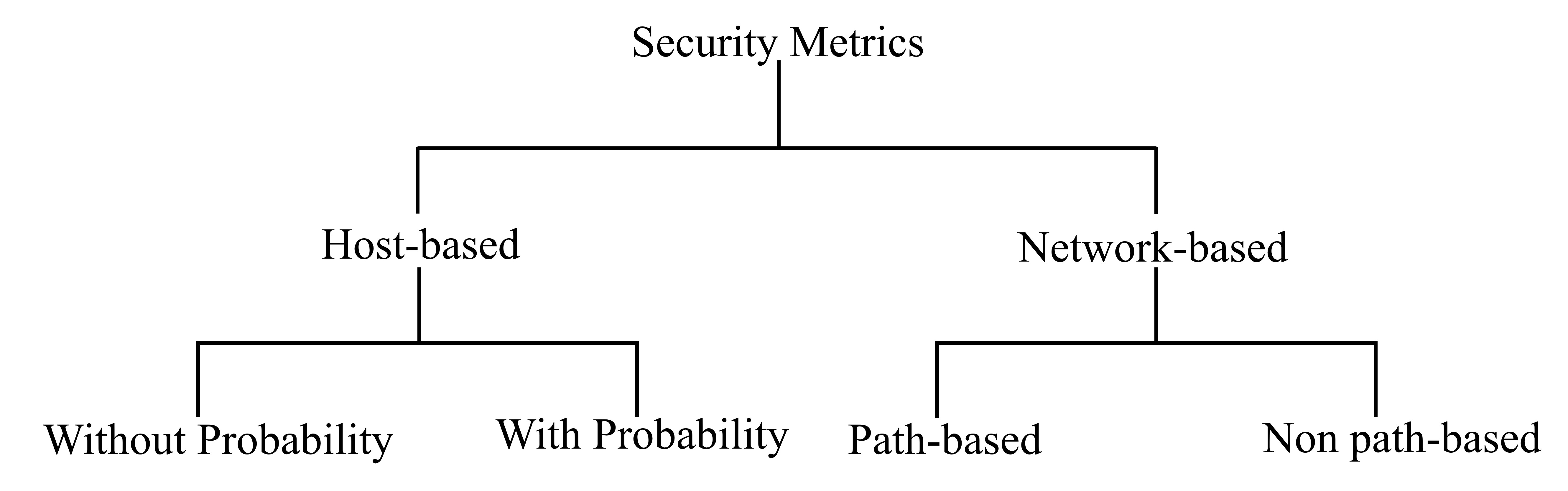
Figure 1: Classification of Security Metrics.

The host-level metrics do not use any network level information (e.g., reachability, protocols, etc) whereas the network-level metrics take into account network structure, protocol and reachability information to quantify the security of a system. We describe the host-level metrics in Section 3.1 and the network-level metrics in Section 3.2, respectively.

3.1 Host-based Security Metrics

The host-level metrics are used to quantify the security level of individual hosts in a network. We further classify the host-level metrics into two types: “without probability” and “with probability”. The reasons for this classification are: (i) sometimes it is infeasible to find a probability value for an attack, and (ii) some analysis and optimisation can be done with or without probability assignments as described in [34].

3.1.1 Metrics without probability values

We summarise the metrics “without probability” in Table 1. Examples of metrics without probability values are attack impact, attack cost, structural important measured [33], mincut analysis [33], mean-time-to-compromise (MTTC)[20, 10], mean-time-to-recovery (MTTR) [16], Mean-Time-to-First-Failure (MTFF) [35], Mean-Time-to-Breach (MTTB)[17], The return on investment [4], The return on attack [4], etc.

Table 1: Description of Metrics without Probability Values.

Metrics	Description
Attack Cost [33]	is the cost spent by an attacker to successfully
	exploit a vulnerability (i.e., security weakness)
	on a host.
Attack Impact [13]	is the quantitative measure of the potential
	harm caused by an attacker to exploit a
	vulnerability.
Mean-time-to-Compromise (MTTC)[20, 10]	is used to measure how quickly a network can
	be penetrated. This type of metrics produces
	time values as end results.
Structural Important Measure [33]	is used to qualitatively determine the most
	critical event (attack, detection or mitigation)
	in a graphical attack model. This metric is
	useful when the probability of event such as
	attack, detection or mitigation are unknown.
Mean-Time-to-Recovery (MTTR)[16]	is used to assess the effectiveness of a network
	to recovery from an attack incidents. It is
	defined as the average amount of time required
	to restore a system out of attack state. The
	shorter the time, the less impact is the attack
	on the overall performance of the network.
The Return on Attack [4]	is defined as the gain the attacker expects from
	successful attack over the losses he sustains due
	to the countermeasure deployed by his target.
	This security metric is from the attacker
	perspective and it used by organisations to
	evaluate the effectiveness of a countermeasure
	in discouraging a certain type of intrusion
	attempts [4].

3.1.2 Metrics with probability values

Conversely, the security metrics with probability include probability security metric [39], Common Vulnerability Scoring System (CVSS) metrics [6] etc. An attack graph (AG) is an acyclic directed graph to represent all possible ways for an attacker to reach a target vulnerability. Wang et al. [39] proposed an AG-based security metric that incorporates the likelihood of potential multi-step attacks combining multiple vulnerabilities in order to reach the attack goal. We summarise the metrics with probability in Table 2.

Table 2: Description of Metrics with Probability Values.

Metrics	Description
Probability of vulnerability exploited [8]	is used to assess the likelihood of an attacker exploiting a specific vulnerability on a host. This takes into account the severity of the host vulnerability.
Probability of attack detection [33]	is used to assess the likelihood of a countermeasure to successfully identify the event of an attack on a target.
Probability of host compromised [11]	is used to assess the likelihood of an attacker to successfully compromise a target
CVSS [23, 6]	is an industry standard used to assess the severity of computer vulnerabilities. Details of the CVSS probability is provided in [29].

3.2 Network-based Security Metrics

This category of metrics uses the structure of a network to aggregate the security property of the network. We further classify these metrics into two types: path based and non-path based metrics (according to the use of path information).

Table 3: Description of Path based Metrics.

Metrics	Description
Attack Shortest Path [32, 27]	is the smallest distance from the attacker to the
	target. This metric represents the minimum
	number of hosts an attacker will use to
	compromise the target host.
Number of Attack Paths [27]	is the total number of ways an attacker can com-
	promise the target. The higher the number, the
	less secure the network.
Mean of Attack Path Lengths [21]	is the average of all path lengths. It gives the
	expected effort that an attacker may use to
	breach a network policy.
Normalised Mean of Path Lengths [15]	This metric represents the expected number of
	exploits an attacker should execute in order to
	reach the target.
Standard Deviation of Path Lengths[15]	is used to determine the attack paths of interest.
	A path length that is two standard deviations
	below the mean of path length metric is
	considered the attack paths of interest and can
	be recommended to the network administrator for
	monitoring and consequently for patching [15].
Mode of Path Lengths [15]	is the attack path length that occurs most
	frequently. The Mode of Path Lengths metric
	suggests a likely amount of effort an attacker
	may encounter.
Median of Path Lengths [15]	this metric is used by network administrator to
	determine how close is an attack path length
	to the value of the median path length (i.e. path
	length that is at the middle of all the path
	length values). The values that falls below the
	median are monitored and considered for
	network hardening [15].
Attack Resistance Metric [40]	is use to assess the resistance of a network confi-
	guration based on the composition of measures of
	individual exploits. It is also use for assessing and
	comparing the security of different network
	configurations [40].

3.2.1 Non-Path Based Metrics

In non-path based metrics, the structure and attributes of a network are not considered; instead, the security of a network is quantified regardless of the network structure. One example of this type of metrics is Network Compromise Percentage (NCP) metric [22]. The NCP metric is defined in Table 4. This metric indicates the percentage of network assets an attacker can compromise. The aim of the NCP metric is to minimise this percentage. Another example is a set of vulnerabilities that allows an attacker to use them as entry points to a network. For instance, web-services running on a host could be the very first targets for an attacker to compromise. The weakest adversary (WA) metric is also a network based metric that is use to assess the security of a network. In the WA metric, a network configuration that is vulnerable to a stronger set of attribute is define as more secure than a network configuration that is vulnerable to a weaker set of initial attacker attributes [30].

Table 4: Description of Non-Path Based Metrics.

Metrics	Description
Network Compromise Percentage [22]	is the metric that quantifies the percentage of hosts on the network on which an attacker can obtain an user or administration level privilege.
Weakest Adversary [30]	is used to assess the security strength of a network in terms of the weakest part of the network that an attacker can successfully penetrate.
Vulnerable Host Percentage [18]	is used to assess the overall security of a network. This metric quantifies the percentage of hosts with vulnerability on a network. The higher the metric value, the less is the security level of the network.

3.2.2 Path Based Metrics

Path based metrics use the reachability information of a network (for example, reachability between hosts, shortest path from a host X to a host Y, and so on) to quantify the security level of the network. We summarise some of these metrics in Table 3, which include Shortest Path (SP) metrics [32], Number of Paths (NP) metrics [27], Mean of Path Length (MPL) metrics [21], Normalised Mean of Path Lengths (NMPL) Metrics [15], Standard Deviation of Paths Lengths (SDPL) Metrics [15], Mode of Path Lengths (MoPL) Metrics [15] and Median of Path Lengths (MePL) Metrics [15].

4 Network Configurations and System Model

The example network is shown in Figure 2. The network consists of two firewalls with an attacker located outside the network. Here, the firewall 1 is use to allow secure connections from the Internet to the hosts in the network while firewall 2 is use to allow secure connections to the database (i.e., $h_{7}$). We assume the goal of the attacker is to compromise the database. We denote hosts in the network as $h_{i}$, where $i=1,2,3...,n$ (a unique identifier for each host in the network). Table 6 shows the firewall rules used for the example network. For simplicity, we selected only one vulnerabilities for each host in the network from the Common Vulnerabilities and Exposures (CVE) [6] which we list in Table 7.

We use the example network and existing security metrics to perform security assessment via the Hierarchical Attack Representation Model (HARM) [14]. We describe the HARM and assumptions of the example network in Section 4.1 and Section 4.2, respectively.

The example network has a finite set of hosts $H$ and a finite set of vulnerabilities $V$. The following notations are used for the security assessment.

Table 5: Notations for the security assessment.

Notation	Meaning
$AP$	is all possible paths from an attacker to a target
$ap$	is an attack path which includes a sequence of hosts
$f$	is a function that identifies the length of the attack path that occurs most
	frequently
$ac_{h}$	is the minimum cost spent by an attacker who successfully compromises
	the host $h$
$aim_{h}$	is the maximum potential loss caused by an attacker who successfully
	compromises the host $h$
$pr_{h}$	is the probability of an attacker to successfully compromise the host $h$
$ac_{ap}$	is the minimum cost spent by an attacker who successfully compromises
	an $ap$
$aim_{ap}$	is the maximum potential loss caused by an attacker who successfully
	compromises an $ap$
$pr_{ap}$	is the probability of an attacker to successfully compromise an $ap$
$ap_{{}_{ex}}$	is the attack path that an attacker is attempting to exploit $e_{x}$
$as_{h}$	is the asset value associated with a host $h$
$s_{v}$	is the set of vulnerable hosts

• A graphical security model - HARM denoted as $GSM$

• Each host $h\in H$ has a name $h_{name}$, a vulnerability $v\in V$ and a set of security metrics $h_{metrics}$$\subseteq${$p_{h}$, $iam_{h}$, $ac_{h}$, $mttc_{h}$, $as_{h}$}.

• Each vulnerability $v\in V$ has a name $v_{name}$.

• Each attack path $ap\in AP$ has an index $ap_{index}$.

4.1 The HARM

We use the HARM to analyse the network security. The HARM is a two-layer model in which the upper layer (AG) represents the network reachability information and the lower layer (AT) represents the vulnerability information.

We defined the AT [9] for HARM as a 5-tuple $at=(A,B,c,g,root)$. Here, $A$ is a set of components which are the leaves of $at$ and $B$ is a set of gates which are the inner nodes of $at$. We require $A{\cap}B=\emptyset$ and $root{\in}A{\cup}B$. Function $c$: $B{\rightarrow}\mathcal{P}(A{\cup}B)$ describes the children of each inner node in $at$ (we assume there are no cycles). Function $g$: $B{\rightarrow}\{AND,OR\}$ describes the type of each gate. The representation of the AT $at_{h}$ associated to the host $h$$\in$$H$ is given as $at_{h}$: $A{\subseteq}h_{vuls}$ (where $vuls$ is the host vulnerability). This means that the vulnerabilities of a node are combined using $AND$ and $OR$ gates.

We defined the AG for HARM [9] as a directed graph $ag=(N,E)$ where $N$ is a finite set of components and $E{\subseteq}N{\times}N$ is a set of edges between components.

The HARM of the example network is shown in Figure 2(b). Other graphical security models such as those suggested by Noel and Jajodia [25] and Ou et al.[28] can also be used.

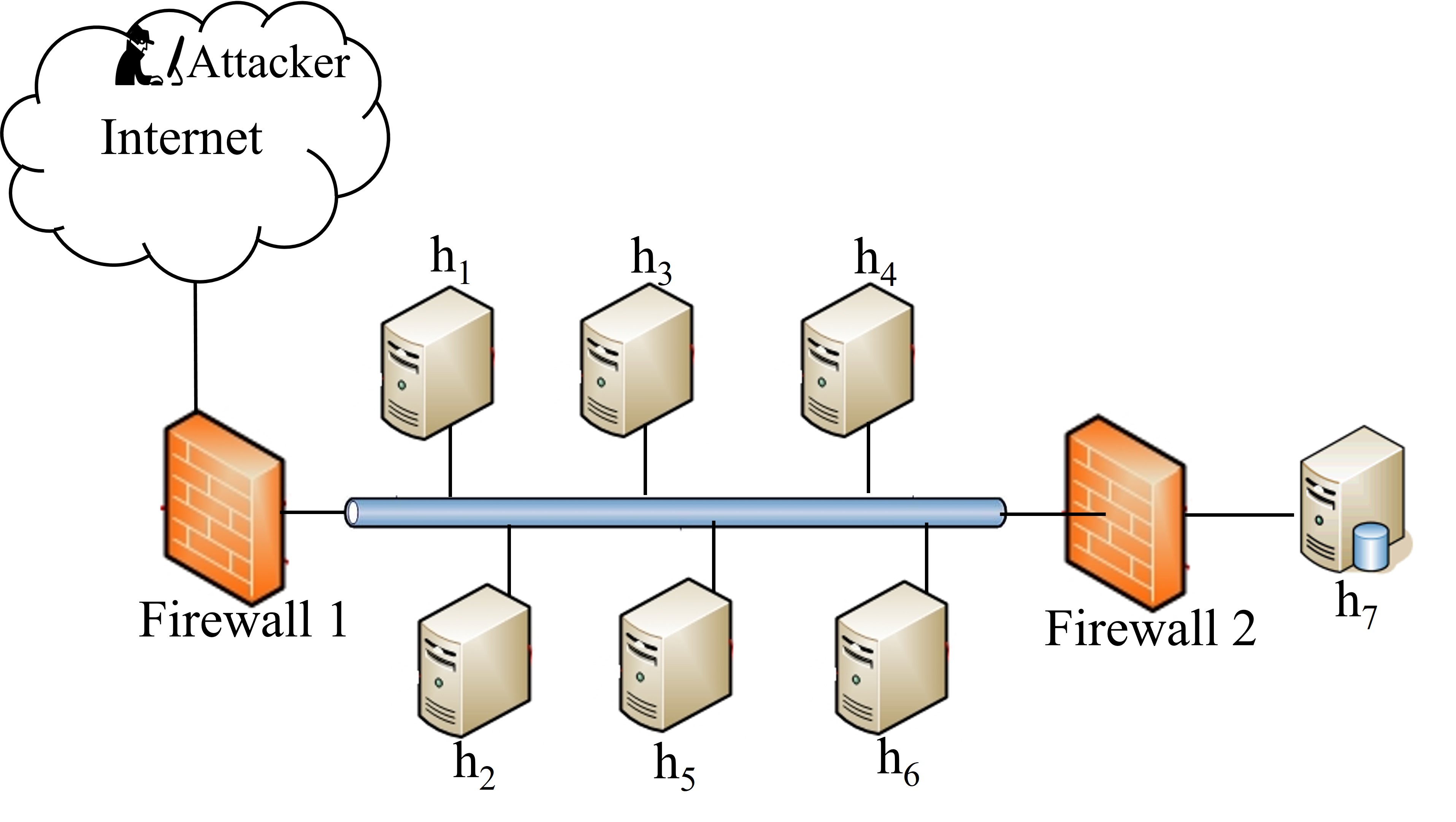
(a) Example Network.

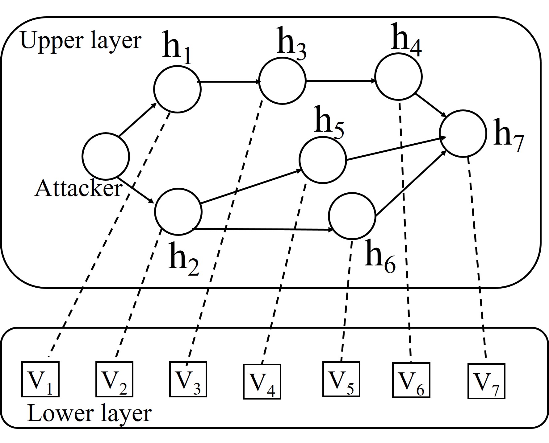
(b) HARM of the Example Network.

Figure 2: An Example Network and the HARM

Table 6: Example network: firewall rules.

Host	accept traffic from
$h_{1}$	Internet
$h_{2}$	Internet
$h_{3}$	$h_{1}$
$h_{4}$	$h_{3}$
$h_{5}$	$h_{2}$
$h_{6}$	$h_{2}$
$h_{7}$	$h_{4}$, $h_{5}$, $h_{6}$

4.2 Assumptions for the example network

We make the following assumptions for the example network:

• An attacker knows the (or has knowledge of) reachability information from the attacker to the target (that is $h_{7}$).

• Each host has only one vulnerability but more vulnerabilities can be modelled as in the work [12, 13].

• Exploiting a vulnerability grants the attacker the root privilege of the host.

• The attacker uses vulnerability scanners such as Nessus [7], Nmap [24], etc to discover all the network vulnerabilities.

4.3 Security Analysis of the Example Network

We use existing security metrics to assess the security of the example network. For simplicity, we selected a few vulnerabilities from the Common Vulnerabilities and Exposures (CVE) [6] which we list in Table 7.

Table 7: List of Vulnerabilities.

h name	v name	CVE-ID	CVSS BS	$pr_{h}$	$aim_{h}$	$ac_{h}$	$as_{h}$
$h_{1}$	$v_{1}$	CVE-2016-2386	7.5	0.75	7	8	40
$h_{2}$	$v_{2}$	CVE-2016-2040	3.5	0.35	4	4.2	21
$h_{3}$	$v_{3}$	CVE-2016-0059	4.3	0.43	5	5 2	25
$h_{4}$	$v_{4}$	CVE-2015-7974	2.1	0.21	3	3.5	17.5
$h_{5}$	$v_{5}$	CVE-2015-2542	9.3	0.93	9	9.2	46
$h_{6}$	$v_{6}$	CVE-2014-2706	7.1	0.71	6.5	7.5	37.5
$h_{7}$	$v_{7}$	CVE-2013-2035	4.4	0.44	4.3	5.5	27.5

In Table 7, the host-based metrics “without probability” values; attack cost and attack impact have metric value of 5.50 and 4.30 for target host $h_{7}$, respectively. These metrics present the minimum cost and the potential loss for the attacker to successfully compromise a host $h_{7}$, respectively. The probability of attack success metric (i.e., a metric “with probability”) is – 0.44. This metric presents the probability that an attacker will successfully exploit the host $h_{7}$. The lower the metric value, is the lower the chances that the attacker will succeed in exploiting the target host.

To calculate the network base metrics, we consider a set of all attack paths $AP$ (i.e. $ap_{1}=(h_{1},h_{3},h_{4},h_{7})$, $ap_{2}=(h_{2},h_{5},h_{7})$, and $ap_{3}=(h_{2},h_{6},h_{7})$) for a given target, $h_{7}$. We compute the network based metrics in Table 8 and Table 9.

Table 8: Metrics Values for “Path based Metrics”.

Metrics Name	Formulae	Value
Shortest Attack Path	$SP(GSM)=\mathop{min}\limits_{ap\in AP}{|ap|}$	3.00
Number of Attack Paths	$NP(GSM)=|AP|$	3.00
Mean of Attack Path Lengths	$MPL(GSM)=\frac{\sum\limits_{ap\in AP}{|ap|}}{NP(GSM)}$	3.30
SDPL	$SDPL(GSM)=\sqrt{\frac{\sum\limits_{ap\in AP}({|ap|}-MPL(GSM))^{2}}{NP(GSM)}}$	0.47
Mode of Path Lengths	$MoPL(GSM)=\mathop{f}\limits_{ap\in AP}{(|ap|)}$	3.00
Attack Resistance	$R(e_{i})=\begin{cases}r(e_{i})+R(e_{j})&\text{conjuctive}\\ \hline\cr r(e_{i})+\frac{1}{R(e_{k})^{-1}+R(e_{l})^{-1}}&\text{disjunctive}\end{cases}$	8.81

In Table 8, the value of the shortest path metric is 3. Based on this metric, an administrator can prioritise the network hardening measure by patching vulnerabilities along the shortest path — in this case, it is the attack path $ap_{2}$ and $ap_{3}$. The number of paths (NP) metric which also yield the value 3.00 indicates the security strength of the network. In the NP metric, the higher the paths number is the lower is the security level. The mean of paths length yield 3.30. This security metrics show the overall network security level. In the mean of path lengths metric, the HARM with higher metric value is recorded as less secure. The standard deviation of path lengths is 0.47. According to this metric, the path length that is two standard deviations below the mean of path lengths metric is considered to be the attacker’s path of interest and regarded as vulnerabilities in hosts along the path are recommended for patching. In this case the $ap_{2}$ and $ap_{3}$ are both two standard deviation below the MPL metric (their two standard deviation value is - 0.64 for both metrics).

To compute the attack resistance metric, two basic operators (disjunctive and conjunctive) described in Wang et al. [40] are used. We compute the attack resistance metric based on the equation provided by Idika [26]. In the equation, the function $r$ represents the difficulty associated with an exploit $e_{m}$. $R$ represent the cumulative resistance of an exploit $e_{m}$ by taking into account all resistance values for ancestors of $e_{m}$. We use each host vulnerability value as the exploit value. In our calculation, the attack resistance value is 8.81. This metric value indicates the network security level and the ability of the network configuration to resist attack.

Table 9: Metrics Values for “non-path based metrics”.

Metrics Name	Formulae	Value
Network Compromise Percentage	$NCP(GSM)=100\times\frac{\sum\limits_{h\in ap_{{}_{ex}}}as_{h}}{\sum\limits_{h\in AP}as_{h}},ap_{{}_{ex}}\in AP$	51.23%
Vulnerable Host Percentage	$VHP(GSM)=100\times\frac{\sum\limits_{h\in s_{v}}h}{\sum\limits_{h\in AP}h},s_{v}\in AP$	100%

In Table 9, we compute the NCP metric. The NCP security metric is for an AG that is not target oriented. In the NCP computation, we assume the attacker is attempting to compromise the set of machines on $ap_{1}$. In our computation, the NCP metric yields a value of 51.23%. In the NCP metric the more machines are compromised, the higher the NCP value. Hence, the goal of the administrator is to reduce the NCP value. The vulnerable host percentage metric yield a value of 100%. This is because all host in our example network has one vulnerability. This security metric is used to compute the percentage of host on a network that have at least one vulnerability.

5 Composite Security Metrics

We propose an approach to develop new set of cyber security metrics called composite security metrics. In these metrics, we combine individual metrics to create a new metric (for example, we can combine attack impact and attack path metric to form the impact on attack path metric, see Figure 3 for more examples). We will use the example network in Figure 2 to perform security analysis using the composite security metrics. We demonstrate our proposed composite metrics using four examples: (i). Impact on attack paths (ii). Risk on attack paths (iii). Return on attack paths (iv). Probability of attack success on paths

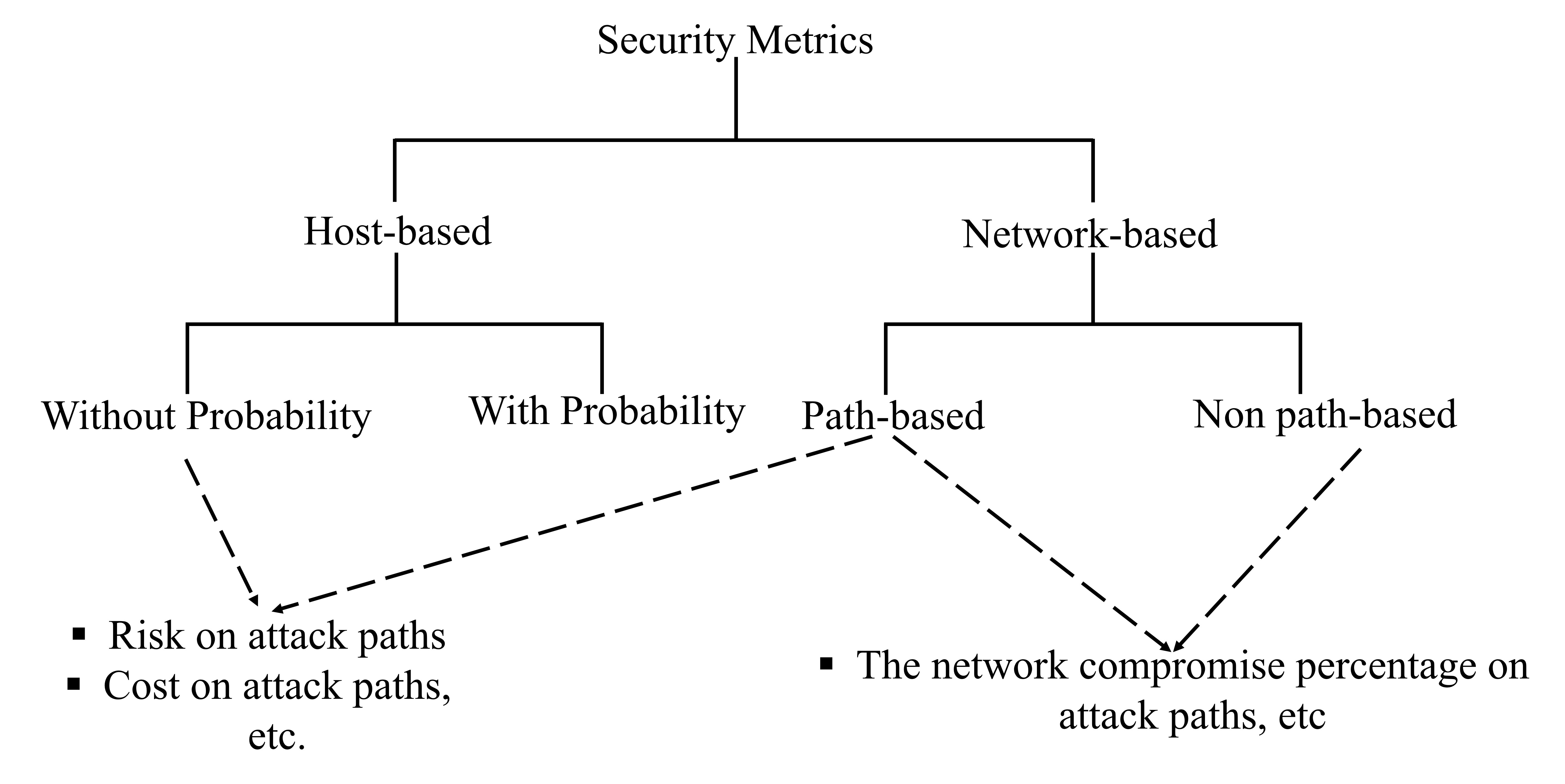
Figure 3: Examples of composite security metrics.

5.1 Impact on Attack Paths

The native metric (as one of the path-based metrics) used to create the impact of paths is attack paths. We combine the attack path metrics with the impact of each host in the path. We define the impact on attack path as the cumulative quantitative measure of potential harm in an attack path. We denote the metric as $AIM$ and calculate it using Equation (3) and (4). The host attack impact is calculated by equation (2). The network-level value $AIM$ is then given by Equation (4).

$$aim_{b}=\left\{\begin{array}[]{ll}\sum\limits_{a\in c(b)}{aim_{a}},&b\in B\atop g(b)=AND\\ \mathop{max}\limits_{a\in c(b)}{aim_{a}},&b\in B\atop g(b)=OR\end{array}\right.$$ (1)

$$aim_{h}=aim_{root}$$ (2)

$$\begin{array}[]{ll}aim_{ap}=\sum\limits_{h\in ap}{aim_{h}},&ap\in AP\end{array}$$ (3)

$$AIM=\mathop{max}\limits_{ap\in AP}{aim_{ap}}$$ (4)

The impact on path metric can reveal the impact of damage associated with each attack path. A security administrator can use this metric to determine which path to patch first. For instance, hosts in the path with the highest impact value can be considered as the prioritised set of hosts to patch.

Using the example network, we use all the possible AP from Figure 2 to compute the impact of path metrics.

$$aim_{ap_{1}} =aim_{h_{1}}+aim_{h_{3}}+aim_{h_{4}}+aim_{h_{7}}$$

$$=7+5+3+4.3$$

$$=19.3$$

$$aim_{ap_{2}} =aim_{h_{2}}+aim_{h_{5}}+aim_{h_{7}}$$

$$=4+9+4.3$$

$$=17.3$$

$$aim_{ap_{3}} =aim_{h_{2}}+aim_{h_{6}}+aim_{h_{7}}$$

$$=4+6.5+4.3$$

$$=14.8$$

The $AIM$ of the example network is 19.3. More detail of how to get the CVSS impact values can be found in [5].

5.2 Risk on Attack Paths

The Risk on attack paths is defined as the expected value of the impact on an attack path. It is computed as the summation of the product of the probability of attack success $pr_{h}$ and the amount of damage $aim_{h}$ h belonging to an attack path ap. The metric is denoted as $R$ and calculate it using Equation (8). The host risk metric is defined by equation (6). The network-level value $R$ is then given by Equation (8).

$$r_{b}=\left\{\begin{array}[]{ll}\sum\limits_{a\in c(b)}{pr_{a}\times aim_{a}},&b\in B\atop g(b)=AND\\ \mathop{max}\limits_{a\in c(b)}{pr_{a}\times aim_{a}},&b\in B\atop g(b)=OR\end{array}\right.$$ (5)

$$r_{h}=r_{root}$$ (6)

$$\begin{array}[]{ll}r_{ap}=\sum\limits_{h\in ap}{pr_{h}\times aim_{h}},&ap\in AP\end{array}$$ (7)

$$R=\mathop{max}\limits_{ap\in AP}{r_{ap}}$$ (8)

We compute the risk of paths metric for all the possible attack paths as follows:

$$r_{ap_{1}} =pr_{h_{1}}\times aim_{h_{1}}+pr_{h_{3}}\times aim_{h_{3}}+pr_{h_{4}}\times aim_{h_{4}}+pr_{h_{7}}\times aim_{h_{7}}$$

$$=(0.75\times 7)+(0.43\times 5)+(0.21\times 3)+(0.44\times 4.3)$$

$$=9.92$$

$$r_{ap_{2}} =pr_{h_{2}}\times aim_{h_{2}}+pr_{h_{5}}\times aim_{h_{5}}+pr_{h_{7}}\times aim_{H_{7}}$$

$$=(0.35\times 4)+(0.93\times 9)+(0.44\times 4.3)$$

$$=11.66$$

$$r_{ap_{3}} =pr_{h_{2}}\times aim_{h_{2}}+pr_{h_{6}}\times aim_{h_{6}}+pr_{h_{7}}\times aim_{h_{7}}$$

$$=(0.35\times 4)+(0.71\times 6.5)+(0.44\times 4.3)$$

$$=7.91$$

This metric shows the level of risk associated with each attack path. From our computed example HARM, the attack path $ap_{2}$ (it’s risk is 11.66) is considered as the path with the highest risk.

5.3 Return on Attack Paths

The return on attack [4] is a metric used to quantify the benefit for the attacker. A return on attack paths computes the benefit for an attacker when the attacker successfully exploits all the vulnerabilities on a particular attack path. From the defender’s point of view, the network administrator can use this metric to reduce the attacker’s benefit by patching vulnerabilities on the path(s) with a high value of ROA. We denote the metric as $ROA$ and it is calculated using Equation (12). The host return on attack metric is given by equation (10). The network-level value $ROA$ is then given by Equation (12).

$$roa_{b}=\left\{\begin{array}[]{ll}\sum\limits_{a\in c(b)}{\frac{pr_{a}\times aim_{a}}{ac_{a}}},&b\in B\atop g(b)=AND\\ \mathop{max}\limits_{a\in c(b)}{\frac{pr_{a}\times aim_{a}}{ac_{a}}},&b\in B\atop g(b)=OR\end{array}\right.$$ (9)

$$roa_{h}=roa_{root}$$ (10)

$$\begin{array}[]{ll}roa_{ap}=\sum\limits_{h\in ap}{\frac{pr_{h}\times aim_{h}}{ac_{h}}},&ap\in AP\end{array}$$ (11)

$$ROA=\mathop{max}\limits_{ap\in AP}{roa_{ap}}$$ (12)

We show how to compute return on attack paths below:

$$roa_{ap_{1}} =\frac{pr_{h_{1}}\times aim_{h_{1}}}{ac_{h_{1}}}+\frac{pr_{h_{3}}\times aim_{h_{3}}}{ac_{h_{3}}}+\frac{pr_{h_{4}}\times aim_{h_{4}}}{ac_{h_{4}}}+\frac{pr_{h_{7}}\times aim_{h_{7}}}{ac_{h_{7}}}$$

$$=\frac{0.25\times 7}{8}+\frac{0.57\times 5}{5}+\frac{0.79\times 3}{3.5}+\frac{0.56\times 4.3}{5.5}$$

$$=1.91$$

$$roa_{ap_{2}} =\frac{pr_{h_{2}}\times aim_{h_{2}}}{ac_{h_{2}}}+\frac{pr_{h_{5}}\times aim_{h_{5}}}{ac_{h_{5}}}+\frac{pr_{h_{7}}\times aim_{h_{7}}}{ac_{h_{7}}}$$

$$=\frac{0.65\times 4}{4.2}+\frac{0.07\times 9}{9.2}+\frac{0.56\times 4.3}{5.5}$$

$$=1.12$$

$$roa_{ap_{3}} =\frac{pr_{h_{2}}\times aim_{h_{2}}}{ac_{h_{2}}}+\frac{pr_{h_{6}}\times aim_{h_{6}}}{ac_{h_{6}}}+\frac{pr_{h_{7}}\times aim_{h_{7}}}{ac_{h_{7}}}$$

$$=\frac{0.65\times 4}{4.2}+\frac{0.29\times 6.5}{7.5}+\frac{0.56\times 4.3}{5.5}$$

$$=1.30$$

Return on attack paths quantifies the network security level from the attacker’s perspective. From the example network scenario, the attack path $ap_{1}$ with metrics value 1.91 has the highest benefit to the attacker.

5.4 Probability of Attack Success on Paths

The probability of attack success on paths is developed by combining path and probability of attack success. The probability of attack success on paths represents the chances of an attacker successfully reaching the target through an attack path. It is calculated by the equation (16) The host attack success probability is defined by equation 14. We denote probability of attack success on paths as $Pr$. The network-level value $Pr$ is then given by Equation (16).

$$pr_{b}=\left\{\begin{array}[]{ll}\prod\limits_{a\in c(b)}{pr_{a}},&b\in B\atop g(b)=AND\\ 1-\prod\limits_{a\in c(b)}(1-pr_{a}),&b\in B\atop g(b)=OR\end{array}\right.$$ (13)

$$pr_{h}=pr_{root}$$ (14)

$$\begin{array}[]{ll}pr_{ap}=\prod\limits_{h\in ap}{pr_{h}},&ap\in AP\end{array}$$ (15)

$$Pr=\mathop{max}\limits_{ap\in AP}{pr_{ap}}$$ (16)

We show how to compute the probability of attack success on paths below:

$$pr_{ap_{1}} =pr_{h_{1}}\times pr_{h_{3}}\times pr_{h_{4}}\times pr_{h_{7}}$$

$$=0.75\times 0.43\times 0.21\times 0.44$$

$$=0.03$$

$$pr_{ap_{2}} =pr_{h_{2}}\times pr_{h_{5}}\times pr_{h_{7}}$$

$$=0.35\times 0.93\times 0.44$$

$$=0.14$$

$$pr_{ap_{3}} =pr_{h_{2}}\times pr_{h_{6}}\times pr_{h_{7}}$$

$$=0.35\times 0.71\times 0.44$$

$$=0.11$$

In this scenario, $ap_{2}$ with metric value 0.14 has the highest probability of a successful attack and therefore it is the $Pr$. The closer the $Pr$ value is to 1, the higher is the likelihood that an attacker will succeed in exploiting the target.

6 Conclusions and Future Work

In this paper, we have described the existing security metrics for cyber security assessment. We have used the network structure and reachability information to classify the existing metrics into host and network based security metrics. We also use the existing security metrics to carry out security analysis. In addition, we described an approach to developing composite security metrics and finally, we formally defined some composite security metrics.

Our classification of security metrics does not capture dynamic security metrics. Thus, we need to incorporate the dynamic security metrics into the proposed classification.

References

- [1] A. Avizienis, J. C. Laprie, B. Randell, and C. Landwehr. Basic Concepts and Taxonomy of Dependable and Secure Computing. IEEE Transactions on Dependable and Secure Computing, 1(1):11–33, Jan 2004.
- [2] C. Barker. NIST Security Measurement NIST SP 800-55 Revision 1, 2007 (accessed February 20, 2016). http://csrc.nist.gov/groups/SMA/ispab/documents/minutes/2007-09/Barker_ISPAB_Sept2007-SP800-55R1.pdf.
- [3] CIS. The Center for Internet Security: Security Metrics, 2010 (accessed February 20, 2016). https://benchmarks.cisecurity.org/tools2/metrics/CIS_Security_Metrics_v1.1.0.pdf.
- [4] M. Cremonini and P. Martini. Evaluating Information Security Investments from Attackers Perspective: The Return-On-Attack (ROA). In Fourth Workshop on the Economics of Information Security, June 2005.
- [5] CVSS. CVSS Calculator, 2016 (accessed February 27, 2016). https://nvd.nist.gov/CVSS-v2-Calculator/CVSS-v2-Equations.
- [6] CVSS. Forum for Response and Security Team, 2016 (accessed February 3, 2016). https://www.first.org/cvss.
- [7] R. Deraison. Nessus Scanner, (accessed February 3, 2016). http://nmap.org/index.html.
- [8] K. A. Edge. A Framework for Analyzing and Mitigating the Vulnerabilities of Complex Systems via Attack and Protection Trees. Ph.D. Air Force Institute of Technology, 2007.
- [9] M. Ge, J. B. Hong, W. Guttmann, and D. S. Kim. A Framework for Automating Security Analysis of the Internet of Things . Journal of Network and Computer Applications, 83:12 – 27, 2017.
- [10] M. Ge and D. S. Kim. A Framework for Modeling and Assessing Security of the Internet of Things. In Proceedings 21st International Conference on Parallel and Distributed Systems (ICPADS), 2015 IEEE , pages 776–781, Dec 2015.
- [11] J. Homer, S. Zhang, X. Ou, D. Schmidt, Y. Du, S. R. Rajagopalan, and A. Singhal. Aggregating Vulnerability Metrics in Enterprise Networks Using Attack Graphs. J. Comput. Secur., 21(4):561–597, July 2013.
- [12] J. Hong and D. S. Kim. HARMs: Hierarchical Attack Representation Models for Network Security Analysis. In Proc. of the 10th Australian Information Security Management Conference on SECAU Security Congress (SECAU 2012), 2012.
- [13] J. B. Hong. Scalable and Adaptable Security Modelling and Analysis. University of Canterbury, PhD Thesis -Computer Science and Software Engineering Department, 2015.
- [14] J. B. Hong and D. S. Kim. Assessing the Effectiveness of Moving Target Defenses Using Security Models. IEEE Transactions on Dependable and Secure Computing, 13(2):163–177, March 2016.
- [15] N. Idika and B. Bhargava. Extending Attack Graph-based Security Metrics and Aggregating their Application. IEEE Transactions on Dependable and Secure Computing, 9(1):75–85, Febuary 2012.
- [16] A. Jaquith. Replacing Fear, Uncertainty, and Doubt. Addison-Wesley, Pearson Education, Indiana, USA, 2007.
- [17] E. Jonsson and T. A. Olovsson. A Quantitative Model of the Security Intrusion Process Based on Attacker Behavior. IEEE Transactions on Software Engineering, 23(4):235 – 245, April 1997.
- [18] A. Kott, C. Wang, and R. F. Erbacher. Cyber Defense and Situational Awareness. Springer International Publishing, 2014.
- [19] L. Krautsevich, F. Martinelli, and A. Yautsiukhin. Formal Analysis of Security Metrics and Risk. Springer Berlin Heidelberg, Berlin, Heidelberg, 2011.
- [20] D. J. Leversage and E. J. Byres. Estimating a Systems Mean Time to Compromise. IEEE Security and Privacy, 6(1):52–60, February 2008.
- [21] W. Li and R. Vaughn. Security Research Involving the Modeling of Network Exploitations Graphs. In Proceedings of sixth IEEE International Symposium Cluster Computing and Grid Workshops. IEEE, 2006.
- [22] R. Lippmann, K. Ingols, C. Scott, K. Piwowarski, K. Kratkiewics, M. Artz, and R.Cunningham. Validating and Restoring Defense in Depth using Attack Graphs. In Proceedings of Military Communications Conference, pages 31–38, 2006.
- [23] P. Mell, K. Scarforne, and S. Romanosky. A Complete Guide to the Common Vulnerability Scoring System (CVSS). http://www.first.org/cvss/cvss-guide.html.
- [24] Nmap. Nmap-network mapper, (accessed February 3, 2016). http://nmap.org/index.html.
- [25] S. Noel and S. Jajodia. Measuring Security Risk of Networks using Attack Graphs. International Journal of Next-Generation Computing, 1(1):135–147, July 2010.
- [26] I. Nwokedi. Characterizing and Aggregating Attack Graph-Based Security Metrics. Ph.D. Thesis, Purdue University, West Lafayette, 2010.
- [27] R. Ortalo, Y. Deswarte, and M. Kaaniche. Experimenting with Quantitative Evaluation tools for Monitoring Operational Security. IEEE Transactions on Software Engineering, 25(5):633–650, 1999.
- [28] X. Ou, W. F. Boyer, and M. A. McQueen. A Scalable Approach to Attack Graph Generation. In Proc. of the 13th ACM Conference on Computer and Communications Security (CCS), pages 336 – 345. ACM, 2006.
- [29] X. Ou and A. Singhal. Quantitative Security Risk Assessment of Enterprise Networks. Springer-Verlag New York, 2011.
- [30] J. Pamula, S. Jajodia, P. Ammann, and V. Swarup. A Weakest Adversary Security Metrics for Network Configuration Security Analysis. In Proceedings of Second ACM Workshop Quality of Protection, pages 31–38. ACM, 2006.
- [31] M. Pendleton, R. Garcia-Lebron, and S. Xu. A Survey on Security Metrics. CoRR, arXiv:1601.05792v1, 2016.
- [32] C. Phillips and L. P. Swiler. A Graph-based System for Network Vulnerability Analysis. In Proceedings of the 1998 workshop on New Security paradigms, pages 71–79. ACM, 1998.
- [33] A. Roy, D. S. Kim, and K. S. Trivedi. ACT: Towards Unifying the Constructs of Attack and Defense Trees. Journal of Security and Communication Networks, 5(8):929–943, 2012.
- [34] A. Roy, D. S. Kim, and K. S. Trivedi. Scalable Optimal Countermeasure Selection using Implicit Enumeration on Attack Countermeasure Trees. In Proceeedings of the 42nd Annual IEEE/IFIP International Conference on Dependable Systems and Networks (DSN), pages 1 – 12. IEEE, 2012.
- [35] K. Sallhammar, B. E. Helvik, and S. J. Knapskog. On Stochastic Modeling for Integrated Security and Dependability Evaluation. Journal of Networks, 1(5):31–42, October 2006.
- [36] R. Savola. Towards a Security Metrics Taxonomy for the Information and Communication Technology Industry. In International Conference on Software Engineering Advances, pages 60–60, Aug 2007.
- [37] R. M. Savola. Towards a Taxonomy for Information Security Metrics. In Proceedings of the 2007 ACM Workshop on Quality of Protection, QoP ’07, pages 28–30, New York, NY, USA, 2007. ACM.
- [38] R. Vaughn, D. Dampier, and A. Siraj. Information Security System Ranking and Rating. CrossTalk the Journal of Defense Software Engineering, 2002.
- [39] L. Wang, T. Islam, T. Long, A. Singhal, and S. Jajodia. An Attack Graph Based Probabilistic Security Metrics. In Proceeedings of the 22nd Annual IFIP WG 11.3 Working Conference on Data and Applications Security, pages 283 – 296. ACM, 2008.
- [40] L. Wang, A. Singhal, and S. Jajodia. Measuring the Overall Network Security of Network Configurations Using Attack Graph. In Proceedings of 21st Annual IFIP WG.3 Working Conference on Data and Applications Security, 2007.