Analytics of Longitudinal System Monitoring Data for Performance Prediction

Abstract

In recent years, several HPC facilities have started continuous monitoring of their systems and jobs to collect performance-related data for understanding performance and operational efficiency. Such data can be used to optimize the performance of individual jobs and the overall system by creating data-driven models that can predict the performance of pending jobs. In this paper, we model the performance of representative control jobs using longitudinal system-wide monitoring data to explore the causes of performance variability. Using machine learning, we are able to predict the performance of unseen jobs before they are executed based on the current system state. We analyze these prediction models in great detail to identify the features that are dominant predictors of performance. We demonstrate that such models can be application-agnostic and can be used for predicting performance of applications that are not included in training.

I Motivation

Run-to-run variability in the performance of parallel codes running on production high performance computing (HPC) platforms is a real problem [1, 2, 3]. Figure 1 shows the varying performance of two HPC applications, Algebraic Multigrid (AMG) and MIMD Lattice Computation (MILC), in spite of running the same executable and input. This variability occurs either due to operating system noise impacting compute regions in the code or due to varying load on shared resources such as the network or filesystem because of changing workloads on the system. There are several ways to mitigate the former but diagnosing and mitigating the impact of the latter is still a challenge on most HPC systems.

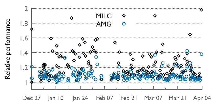
Figure 1: Variability in the performance of 128-node AMG and MILC jobs on different days (on Cori at NERSC).

Sharing of network or filesystem resources by all concurrently running jobs leads to uneven resource usage over time, which can impact performance reproducibility. For individual HPC users, reducing performance variability leads to predictable performance, faster scientific results, and reduced allocation costs. At an administrative level, better performance of individual jobs leads to both energy savings and higher job throughout.

In recent years, several HPC facilities have started continuous monitoring of their systems and jobs to collect performance-related data for understanding performance and operational efficiency.  [4]. Analyzing such data and using it for data-driven modeling can help us understand the causes of performance variability and guide us in developing techniques to mitigate it. For example, an intelligent software stack can use modeling to predict the runtime of pending jobs in the queue and use those models to adapt scheduling decisions to mitigate performance variability.

Recent advances in machine learning approaches are driving scientific discovery across many disciplines – this presents a unique opportunity in the HPC community to remove human associated guesswork in the performance engineering loop, and instead, use data-driven ML models for performance modeling, forecasting, and tuning. Analytics of performance-related data can help in identifying performance anomalies and their root causes, in modeling and forecasting performance, and ultimately, in providing insights that can translate into actions for correcting inefficient behavior.

In this paper, we analyze longitudinal system monitoring data to explore the causes of performance variability in certain control jobs. The monitoring data is collected by the Lightweight Distributed Metric Service (LDMS) on Cori, a $\scriptstyle\mathtt{\sim}$30 Pflop/s Cray XC40 system at NERSC. Analyzing system-wide monitoring data gives us a global view of the system, a perspective which users running individual jobs do not have. Separately, we also run some control jobs on Cori to document the impact of varying resource usage on application performance. Our goal is to analyze system state before a job starts executing and use that data to create a model that can predict the performance of future jobs based on the system state at that time.

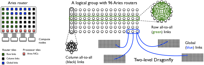
Figure 2: Network ports classified into router and processor tiles on the 48-port Aries router (left) and a multi-group dragonfly system constructed using the Aries router as a building block (right).

We use machine learning, specifically regression models, to model the execution time of jobs in terms of several network related hardware counters gathered by LDMS. We use these models to understand which hardware counters are strong predictors of performance, in other words, indicators of performance degradation. We demonstrate that our data-driven modeling approach that uses past system state is successful in performance prediction of unseen data – i.e. new pending jobs in the queue.

Our work makes the following important contributions:

• We create a pipeline to process, filter and aggregate large-scale system-wide monitoring data to make it suitable for consumption by machine learning (ML) models.

• We develop ML-based regression models that can predict the performance of unseen jobs using past system state.

• We analyze feature importances in different models to identify strong predictors of performance degradation.

• We demonstrate that such models can be application-agnostic and can be used for predicting performance of applications that are not included in training.

II Background and Related Work

In this paper, we analyze system-wide monitoring data gathered on a Cray XC40 system, and analyze performance variability arising due to network sharing. Hence, we provide a brief overview of the Cray XC40 dragonfly network and resource management on such systems.

II-A Overview of the Cray XC40 system

The Cray XC40 system is the older generation of dragonfly-based systems [5] that use the Aries router. The Aries router has 48 ports that are used to connect to compute nodes and other routers on the network. Eight ports referred to as processor tiles are used to connect to four compute nodes (as shown in Figure 2). The remaining 40 ports are referred to as router tiles and are used to connect to other routers. 96 Aries routers are connected in a 16 $\times$ 6 rectangular grid to form a logical group. In a group, each router is directly connected to every other router in its row and every other router in its column. The remaining ports after connecting to routers in the group are used for global links which connect to routers in other groups throughout the system.

II-B Resource Management and Sources of Variability

On most HPC systems, job schedulers assign any available nodes to ready jobs in the queue without regard to their location in the physical network topology. Cray dragonfly-based systems are no exception to this. Smaller jobs may be spread over fewer groups and routers, whereas larger jobs may be spread over more groups. However, there are no guarantees provided by the job scheduler as to the compactness of a job allocation. Hence, a job may share routers and groups with other jobs. Compute nodes are always dedicated to individual jobs but the network and filesystem are shared by all concurrently running jobs.

In principle, the compactness of a job should have no bearing on its communication or overall runtime because adaptive indirect routing deployed on these systems should distribute traffic evenly over all global links [6]. In practice, significant performance variability can be observed when the same executable is run on a dragonfly system repeatedly. This paper primarily considers the effect of traffic on the interconnection network on such variability. Traffic on the network consists of intra-job communication, for example MPI messages, or traffic to/from the filesystem during input/output (I/O) operations from all running jobs. Even in absence of OS noise, this resource sharing by all jobs can have a significant performance impact.

TABLE I: Description of raw network hardware performance counters gathered by LDMS

	Raw counter name	Description
	AR_RTR_INQ_PRF_INCOMING_FLIT_VCv	Number of flits received on virtual channel v of a router tile
	AR_RTR_INQ_PRF_INCOMING_PKT_VCv	Number of cycles stalled on a virtual channel v of a router tile
	AR_RTR_INQ_PRF_ROWBUS_STALL_CNT	Total number of cycles stalled on a router tile
	AR_NL_PRF_REQ_NIC_n_TO_PTILES_FLITS	Number of NIC request flits from NIC n to all processor tiles
	AR_NL_PRF_REQ_PTILES_TO_NIC_n_FLITS	Number of NIC request flits from all processor tiles to NIC n
	AR_NL_PRF_RSP_NIC_n_TO_PTILES_FLITS	Number of NIC response flits from NIC n to all processor tiles
	AR_NL_PRF_RSP_PTILES_TO_NIC_n_FLITS	Number of NIC response flits from all processor tiles to NIC n
	AR_NL_PRF_REQ_NIC_n_TO_PTILES_STALLED	Number of clock cycles requests from NIC n have stalled to all processor tiles
	AR_NL_PRF_REQ_PTILES_TO_NIC_n_STALLED	Number of clock cycles requests from all processor tiles have stalled to NIC n
	AR_NL_PRF_RSP_NIC_n_TO_PTILES_STALLED	Number of clock cycles responses from NIC n have stalled to all processor tiles
	AR_NL_PRF_RSP_PTILES_TO_NIC_n_STALLED	Number of clock cycles responses from all processor tiles have stalled to NIC n

II-C Related Work

Performance variability refers to the variation in total job runtime of the same application with the same or similar inputs. Several studies have established the order of magnitude difference between identical executions of the same HPC program [1, 2, 7, 3]. Petrini et al. [1] highlight the role of operating system daemons in creating noise or jitter and in degrading application performance. Hoefler et al. [8] study the impact of OS noise on the performance of large-scale parallel applications.

In recent years, HPC researchers have begun to use the breadth of historical data available due to new comprehensive data gathering at HPC facilities [4, 9]. Lockwood et al. [4] explain performance variation due to changing circumstances in the file system. Tuncer et al. [9] perform classification and detection of anomalous performance based on Aries counters. They use machine learning combined with system data, but primarily focus on diagnosing anomalies in compute node health and not performance of jobs. Agelastos et al. [10] create a HPC system profiler to explain the performance variability of applications across different HPC systems.

Chunduri et al. [11] measure and attribute runtime variation to runtime system state. However, they primarily focus on single node variation using data acquired simultaneously to the running time of a job, whereas we use data strictly before execution and consider all system nodes. Jha et al. [12] investigate the relationship between overall during-run network congestion and performance.

Wolski et al. [13] created a comprehensive system (Network Weather Service) to estimate CPU usage and the throughput of network traffic based on system state. The NWS, while successful, does not consider the same breadth of data nor attempt to predict application runtime. Skinner et al. [14] highlight the impact of cross application contention and parallel filesystem interference on the NERSC IBM SP system (Seaborg). Bhatele et al. [3] use regression models to analyze per-job data combined with system data to predict the overall performance and per time step performance of individual jobs. This paper uniquely looks at predicting the performance of job runtime using only system data strictly before a job’s execution. To the best of our knowledge, this is the first work that analyzes longitudinal system-wide data to predict the performance of pending jobs in the queue.

III Data Description

Below, we describe the LDMS-gathered system-wide data and control jobs’ data used for training ML models. The data was gathered on a Cray XC40 system at the National Energy Research Computing Center (NERSC) named Cori. Cori features 12,076 compute nodes across 34 groups; of these 9,668 nodes are powered by 68-core Intel Xeon Phi Knights Landing (KNL) processors [15].

III-A Longitudinal System Monitoring Data

LDMS provides a framework for system-wide collection of performance related data, albeit at a single frequency configured for the entire system. This may be every second to every minute, depending on the resources available to analyze and store the data. Recently, NERSC systems have begun to run LDMS, collecting network data every second. This volume of data amounts to approximately 5 TB per day, which presents challenges for collection and analysis. Individual HPC users that lack administrative access can collect similar information, albeit for their own routers using the AriesNCL counter library. We now describe what portions of the system-wide data we use in our analysis and how we process the raw data to put it in a form that can be ingested by machine learning models.

Raw LDMS Data: Each Aries router on the Cray XC system has a multitude of hardware counters that track various network events across each router and processor tile [16]. The raw LDMS system data collected on Cori consists of a subset of these hardware counters. These counters are collected for each of the 48 network tiles, across all 2890 routers on the entire system. LDMS gathers this counter information every second and writes it to disk. In this paper, we consider a subset of these counters that we believe to be important indicators of network congestion. The raw counters and their descriptions are listed in Table I.

Data Extraction from Time Series: The raw counter data collected across the entire system is essentially a time series. Since we are interested in predicting the performance of unseen jobs using system data from the recent past, we decided to analyze data from the last five minutes prior to the beginning of execution of each control job (described in the next subsection). For each control job, we filter the time series by only looking at the change in counter values in the last five minutes prior to the start time of a job (see Figure 3). For each job, this gives us a large table of the previously identified network counters and the change in their values in the last five minutes. This data is for each router and network tile on the system. Next, we look at how we further process this data by aggregating it in meaningful ways.

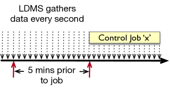
Figure 3: LDMS data five minutes prior to job start is used as input to train the machine learning models.

TABLE II: Description of derived counters used for modeling. Colors in the left column map derived features to raw features in Table I.

	Derived counter name	Abbreviation	Description
	AR_RTR_INQ_PRF_INCOMING_FLIT_REQ	RT_FLIT_REQ	Total number of request flits received on a router tile
	AR_RTR_INQ_PRF_INCOMING_FLIT_RSP	RT_FLIT_RSP	Total number of response flits received on a router tile
	AR_RTR_INQ_PRF_INCOMING_PKT_REQ	RT_PKT_REQ	Total number of cycles requests stalled on a router tile
	AR_RTR_INQ_PRF_INCOMING_PKT_RSP	RT_PKT_RSP	Total number of cycles responses stalled on a router tile
	AR_RTR_INQ_PRF_INCOMING_FLIT_ROW	RT_FLIT_ROW	Total number of flits received on all row links of a router
	AR_RTR_INQ_PRF_INCOMING_FLIT_COL	RT_FLIT_COL	Total number of flits received on all column links of a router
	AR_RTR_INQ_PRF_INCOMING_FLIT_GBL	RT_FLIT_GBL	Total number of flits received on all global links of a router
	AR_RTR_INQ_PRF_ROWBUS_STALL_ROW	RT_STL_ROW	Total number of stalls on all row links of a router
	AR_RTR_INQ_PRF_ROWBUS_STALL_COL	RT_STL_COL	Total number of stalls on all column links of a router
	AR_RTR_INQ_PRF_ROWBUS_STALL_GBL	RT_STL_GBL	Total number of stalls on all global links of a router
	AR_NL_PRF_REQ_FLITS	PT_FLIT_REQ	Total number of NIC request flits on a processor tile
	AR_NL_PRF_RSP_FLITS	PT_FLIT_RSP	Total number of NIC response flits on a processor tile
	AR_NL_PRF_REQ_STALLED	PT_STL_REQ	Total number of cycles requests stalled on a processor tile
	AR_NL_PRF_RSP_STALLED	PT_STL_RSP	Total number of cycles responses stalled on a processor tile

III-B Reduction in Data Dimensionality

The resulting subset extracted from the longitudinal data is still extremely high-dimensional because of counter values being per network tile (port) and per router. We perform aggregations of this data along different axes to get the data in final form:

Reducing Tile Data: We begin by performing reductions across each individual router. Each 48-port Aries router contains 40 router ports that connect to other routers and the remaining eight ports connect to the compute nodes on that router. The aggregation across all router tiles yields the 17 (2 * 8 VCs + row_bus stalls) raw counters that constitute the top section of Table I. A similar reduction across all the processor tiles yields the bottom section of Table I. Following this reduction, we are left with $17+8=25$ raw features across all 2890 routers for each job run in our dataset.

Creating Interpretable Derived Features: Next, we perform a sum over the reduced raw counters to create a set of human interpretable derived features (Table II). For example, incoming flits on virtual channels 0–3 (AR_RTR_INQ_PRF_INCOMING_FLIT_VCv, $v$=0,1,2,3) of a router tile are added together to create the AR_RTR_INQ_PRF_INCOMING_FLIT_REQ feature. Incoming flits on virtual channels 4–7 (AR_RTR_INQ_PRF_INCOMING_FLIT_VCv, $v=4,5,6,7$) of a router tile are added together to create the AR_RTR_INQ_PRF_INCOMING_FLIT_RSP feature (top section of Table II) . Similarly AR_NL_PRF_REQ_NIC_n_TO_PTILES_FLITS and AR_NL_PRF_REQ_PTILES_TO_NIC_n_FLITS for a processor tile are summed together to create the AR_NL_PRF_REQ_FLITS feature (bottom section of Table II). The colors in Table I and II provide a mapping between the raw and derived features. The middle section of Table II represents another way of looking at the counters data. Instead of reducing counters over all router tiles, we reduce the flit and stall counters by the type of link (row, column, or global). This creates the six features in the middle section of Table II. These different derivations yield 14 derived features for each of the 2890 routers.

Filtering by Router Type: Nodes with different functionality such as compute nodes, I/O servers, management and login nodes are attached to different routers. We can either consider all routers or filter by the types of nodes attached to a router. We explored the following groupings, some of which only consider a subset of routers: routers connected to compute nodes (henceforth referred to as all routers), routers attached to nodes that are assigned to the control job (henceforth referred to as my routers), routers that are connected to I/O servers (IO routers), etc. We ultimately chose to feature the results from analyzing data from all routers connected to compute nodes, routers connected to I/O servers and the subset of routers that are attached to nodes assigned to a particular job (my routers). These two groupings yielded the strongest results and are solutions that could be implemented by system administrators and individual users respectively.

Aggregating over Router Types: Once a subset of routers has been selected in accordance to one of the above groupings, we explored various aggregation schemes to aggregate the data across routers for either set of input features (raw or derived). This aggregation calculates one value for each counter by applying one of the following functions over the entire router subset: mean, standard deviation, various percentiles such as median, 75th percentile, 95th percent, and IQR (75th - 25th percentile). We present results for some of these aggregation functions.

III-C Control Jobs Data

Most previous work either analyzes system-wide monitoring data or per-job application data when analyzing performance. In this work, we set up some control jobs that enable us to assess the impact of system state on the performance of production applications. We run three codes – AMG, MILC, and miniVite, which are representative of common workloads on HPC systems. AMG and MILC were run in a weak scaling mode, and hence they performed well on both 128 and 512 nodes. miniVite’s input problem is a fixed-size real world graph and strong scaling the input problem from 128 to 512 nodes led to poor performance. Hence, miniVite was only run on 128 nodes. Each application run was short, running for between five to ten minutes. We briefly describe each application below.

AMG: is a proxy application for parallel algebraic multigrid solvers based on Hypre linear solver library [17]. The input problem runs AMG-GMRES on a linear system for a three-dimensional problem with a problem size of $32\times 32\times 32$ per MPI process.

MILC: refers to MIMD Lattice Computation, primarily used in numerical simulations of quantum chromodynamics. The MILC application, su3_rmd, was used in these experiments, which performs a 4D stencil on a per process grid of dimensions $4\times 4\times 4\times 4$.

miniVite: is a proxy application for Vite [18], and is representative of graph analytics workloads [19]. It performs a single phase of the Louvain classification, which is an algorithm for community detection in large distributed graphs. Graph analytics workloads are seeing increased usage of HPC clusters. An iterative loop was added to miniVite to repeat its work several times.

We submitted control jobs for each application to the production batch queue on Cori between December 2018 and April 2019. All control jobs were run on KNL nodes, alongside jobs of other users on the system. We left 4 out of 68 cores on each node for OS daemons to minimize the effects of OS noise on compute regions in the code. Based on when each job ran, LDMS data was processed to obtain the derived features for the 5-minute interval prior to the execution of the job (Figure 3). We also recorded the execution time for the main execution loop of each application, which is the variable our ML models try to predict. Table III presents the five datasets created for training the models and the number of samples in each dataset. Note that whenever we refer to an application dataset in the paper, it refers to the system-wide data collected from the 5-minute interval prior to the beginning of each job in the dataset and that job’s respective execution time. The models are trained solely on the system-wide data and no application-specific data is used for training.

TABLE III: Applications and node counts used for control jobs

Application	No. of Nodes	Number of jobs
AMG 1.1	128	156
AMG 1.1	512	152
MILC 7.8.0	128	151
MILC 7.8.0	512	153
miniVite 1.0	128	119

Job Placement Data: In addition to the execution times of each job, we also calculate two additional placement features from system job logs. The first, NUM_ROUTERS, indicates the total number of unique routers that a job was assigned nodes on. The second, NUM_GROUPS, indicates how many dragonfly groups these routers were spread across. These features indicate the degree of compactness or spread in terms of placement of each job.

IV Methods for Data Analytics

We now present our approach for creating prediction models, obtaining importance of different features, and evaluating the predictive power of the trained models.

IV-A Machine Learning based Prediction Models

In this work, we utilize gradient boosted regression (GBR) both in our prediction models and for assigning importances to input features. Gradient boosted regressors utilize an ensemble method that assumes that the true regression function is a linear combinations of several different base learners [20, 21]. These base learners typically constitute decision trees, which benefit from higher levels of human interpretability particularly in determining the importances of input features. Given that the number of samples per application is small, we solely consider GBR in our experiments to determine feature importances. However, despite the co-linearity of our input data and smaller dataset sizes, we also observed relative success with Naive Bayes based regression. We may consider using it in future experiments.

In addition to using GBR, we also train a neural network when combining multiple datasets to create application-agnostic models in Section V-C. The larger combined dataset allows for more complex models. We utilize a small neural network consisting of two 8-node hidden layers each with a 50% dropout connected to a final output layer with a linear activation. The dropout layers randomly select 50% of the nodes to exclude from a layer during training and help to reduce overfitting [22]. Gradient boosting regressors can struggle with extrapolation so a neural network was selected to counter this specificity [23].

IV-B Training the Models

In Sections V-A and V-B, we train separate machine learning models for each of the first four datasets in Table III. We perform a 20-fold cross-validation, where the dataset is split into 20 parts randomly. One part is used for testing and the other 19 parts are used for training. The inputs to the ML algorithms for creating the dataset-specific ML models are: (1) for each sample (job) in the training set, values of the counters described in Table I or II for the five minutes prior to the start of that job are provided as the input features, and (2) execution time of each sample (job) is provided as the dependent variable to be modeled. Given a set of samples in the testing set, the model outputs the predicted execution time of each testing sample based on the values of the independent features (counter values) for that sample. We standardize all input features (counter values) and the execution time of the training data (yielding a mean of zero and standard deviation of one for each feature and the output vector). When testing a model, we apply the same standardization vectors obtained from the training data on the test data (to entirely remove any information from the testing set from our pipeline).

In Section V-C, we attempt to create an application-agnostic model that can predict the performance of an arbitrary application not included in the training dataset. We create multiple datasets by combining data from different rows of Table III, and leaving some datasets for testing entirely. For example, in one instance, we combine the following three datasets – AMG 128, AMG 512, and MILC 128, train a model using the combined data, and use the trained model to predict the performance of MILC 512. In a separate study, we combine datasets by application type. For example, we combine all AMG and MILC datasets, train a model, and use miniVite as an unseen testing dataset. Note that when we combine multiple datasets, we standardize their features and execution times separately. We de-normalize the output by using a standardization vector created from the oracle execution times of the testing data. If we were to use such a model for a new application, we would not have a standardization vector for de-normalizing the predicted values. However, the standardized output still allows for the evaluation of relative expected performance and still provides a strong heuristic for overall runtime with only an estimation of the true application runtime distribution.

IV-C Calculating Feature Importances

To analyze the relative importance of the derived system-wide counters in forecasting job runtime, we use the technique of recursive feature elimination (RFE). For each application dataset, we perform a summary across a particular router type using an aggregation function, and train a GBR model. We identify the worst performing feature based on feature importances, drop that feature from the training data, and train again with the smaller set of features. This process continues until all features are eliminated. Finally, based on the ranking of when each feature is eliminated, we select the five best features and compute a relevance score for each selected feature.

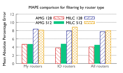
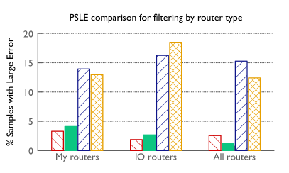
Figure 4: MAPE and PSLE scores for the GBR model when using different router types for filtering the system-wide data.

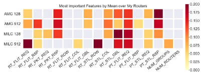
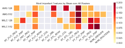
Figure 5: Relative importances of the most important counters obtained using RFE for different datasets (aggregation function: mean).

We use a tree-based feature importance metric for the GBR. For each feature utilized by each of GBR’s decision trees, the total reduction in mean squared error that can be attributed to a branch utilizing that feature is calculated for all features [24]. Note that all input features in our dataset are strictly numeric and thus less susceptible to biases sometimes present in tree-based feature importances. For each dataset, we perform this calculation of feature importances 5-fold and average the results across all validation splits.

IV-D Metrics for Evaluation

We define two metrics that are indicative of usefulness in predicting overall job runtime in practice. The first, mean absolute percentage error (MAPE), calculates the mean of percentage errors observed for each test sample as follows,

$$\mathrm{MAPE}=\frac{1}{n}\sum_{i}^{n}\frac{|y_{i}-\hat{y}_{i}|}{y_{i}}$$

where, $y_{i}$ is the true value, and $\hat{y}_{i}$ is the predicted value.

We also define an additional metric to measure the relative accuracy of our regression models: percent of samples with large error (PSLE). We define a test sample to have a large error if the predicted value is more than $x$% higher than the true value. For the entire dataset, PSLE is defined as,

$$\mathrm{PSLE}=\frac{1}{n}\sum_{i=1}^{n}\mathit{LE}_{i}$$

$$\mathit{LE}_{i}=\begin{cases}1,&\text{if }\frac{|y_{i}-\hat{y}_{i}|}{y_{i}}>x\\ 0,&\text{otherwise}\end{cases}$$

We use $x=0.15$ for the evaluation in this paper. This metric is important because when a system wants to use the model, it may not need exact predictions of the job runtime. It may be more important to predict the general trend i.e. is the next job going to run reasonably fast or unreasonably slow?

V Evaluation of Machine Learning Models

We now evaluate and compare the prediction models generated using datasets based on different router groupings and aggregation functions.

V-A Models based on different router groups

In order to understand the significance of different router groups in predicting performance, we created GBR models for each application dataset using three different router groups – my routers, IO routers, and all compute routers. We observe that despite limiting ourselves to a small number of samples per dataset, all models performed sufficiently well (Figure 4). We see that all router groups are good at predicting AMG performance with MAPE below 5% and for MILC, which has a much higher variance in runtime, all MAPEs are below 10%. The All router grouping is somewhat better than the other two. We see a similar trend with the Percentage Samples with Large Error (PSLE) metric –– for AMG, the models predict worse than 15% for less than 5% of the test data. However, for MILC, PSLE is somewhat higher due to the high variability in the MILC dataset. We also observe that we obtain good scores for both My routers and All routers groupings. This indicates that both system administrators and individual HPC users could see relative success in predicting complex job execution with small temporal information.

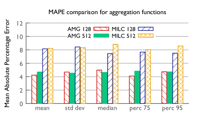
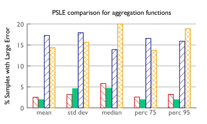
Figure 6: MAPE and PSLE scores for the GBR model when using different aggregation functions over all compute routers.

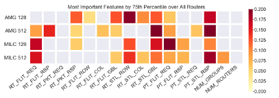
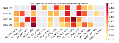
Figure 7: Relative importances of the most important counters obtained using RFE for different datasets (router type: compute routers).

Using recursive feature elimination for both AMG and MILC datasets, we calculated relative importance scores for all input features in the My routers and All routers groupings. In Figure 5, we visualize the feature importances of the derived counters for the four datasets. We observe that the two router groupings rely on some common features – RT_PKT_RSP (stalls on router tiles), RT_STL_GBL (stalls on global links), PT_FLIT_REQ (processor tile flits), and PT_STL_RSP (processor tile stalls).

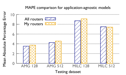
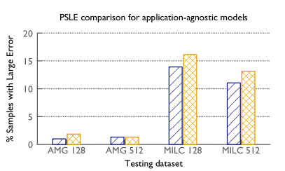
Figure 8: MAPE and PSLE scores for the NN model when using three datasets for training and a fourth disjoint dataset for testing (x-axis label.) The training dataset for each cluster is the combination of AMG 128, AMG 512, MILC 128, MILC 512 minus the dataset in the x-axis label.

V-B Models by different types of aggregation

In the previous section, we used the mean function to aggregate data over all routers in a particular group. We now consider various other aggregation strategies, and the top performing aggregations are shown in Figure 6. We observe that across these top performing aggregation schemes, the prediction scores do not vary significantly for the different applications. In terms of the application of these prediction models in a system-wide job scheduler, we see this as a promising result as the true mean across all routers is not needed. It suggests the potential for strong results using a computationally less-expensive aggregation and highlights the potential of accurate estimation using a small subset of routers.

Next, we perform recursive feature elimination on the derived features using aggregation by 75th percentile. Figure 7 shows the feature importances for the 75th percentile aggregation over My routers and All routers groupings. We see a consistent story in the feature importances to the mean aggregation suggesting a robustness in this ranking strategy. Some of the same derived counters appear to be the most important – RT_PKT_RSP (stalls on router tiles), RT_STL_GBL (stalls on global links), PT_FLIT_REQ (processor tile flits), PT_STL_RSP (processor tile stalls). Note that the NUM_GROUPS feature is also important for the MILC 512 dataset.

V-C Application-agnostic Models

Finally, we analyze the generalizability of the ML algorithms and their prediction models. The end goal is to create a single model that can accurately predict the standardized runtime for any application even if we do not have data for that application in the training dataset. In the first study of generalizability, we use four datasets - AMG 128, AMG 512, MILC 128, and MILC 512. In turns, we use three of these datasets for training and reserve the fourth dataset entirely for testing. We segment the training data into 8-fold cross-validation segments and train a model that can predict the standardized runtime of any job in the testing set given the previous five minutes of system data. Each prediction is later de-normalized with respect to its application and an error metric is calculated for that prediction. For all the results in this section, we use the neural network model, apply the mean function to aggregate the data, and compare the use of data from All routers versus My routers in each case.

Figure 8 shows the success of the trained models in terms of their MAPE and PSLE scores. Comparing with Figure 6, we observe that when combining multiple datasets, the models perform better in terms of predicting the execution times, compared to using the datasets by themselves. The MAPE for predicting AMG 128 reduces from 4.23 to 3.61 and that for AMG 512 from 4.71 to 4.25. Similarly the MAPE for predicting MILC 512 reduces from 8.21 when used by itself for training to 7.5 when the other three datasets are combined for training a model. This improvement is likely due to the larger training dataset ($\scriptstyle\mathtt{\sim}$450 samples versus $\scriptstyle\mathtt{\sim}$150) allowing for more robust training of models. We see this as a promising sign for future models which could include tens of applications with hundreds of samples each and likely even stronger and more generalizable predictions. We also observe that using the data from only the routers allocated to a job does not degrade the models significantly. This suggests that in absence of system-wide data, an end user can work with data from routers that they have access to.

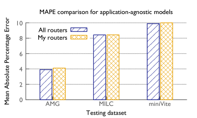
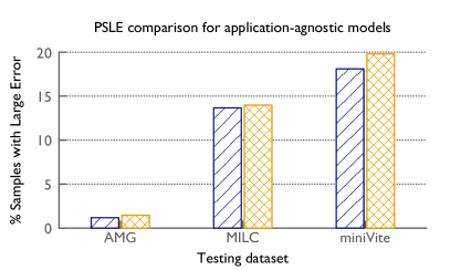
Figure 9: MAPE and PSLE scores for the NN model when combining datasets by application type. Two applications are used for training and the third application is used for testing (x-axis label.)

In the second study of generalizability, we combine datasets by application type and reserve one of the applications as unseen data for testing. For example, when we combine all AMG and MILC datasets for training, we use the miniVite dataset for testing. Figure 9 shows how these application-agnostic models perform in terms of predicting the performance of an unseen application. We observe that AMG has the lowest errors, followed by MILC and then miniVite. On average, AMG has the lowest percentage of communication with respect to its total execution tine, followed by MILC, and then miniVite. This results in AMG having the lowest performance variability and miniVite the highest. We believe that this is the reason for the models having better success with predicting AMG’s performance as opposed to that of MILC and miniVite. Nevertheless, the results are still encouraging. Even without any data for an application being included for training, the ML models demonstrate reasonable success in performance prediction. We expect that as we add more applications with different computation and communication signatures to our training set, the prediction scores for other unseen applications will improve.

Finally, we analyze feature importances when training the neural network model using the combined datasets. Figure 10 shows the relative feature importances for three different training datasets (AMG+MILC, AMG+miniVite, and MILC+miniVite), and two filterings (All routers and My routers). Surprisingly, NUM_GROUPS emerges as a highly important feature. In principle, one would expect that the placement of a job should have little impact on its performance due to adaptive indirect (UGAL) routing [6]. However, in practice, it is possible that when a job is spread over more groups, the likelihood of encountering congestion on global links increases. RT_STL_GBL (stalls on global links) is also important for predicting all three applications as we had observed in the previous sections. We also observe that while applications share common important features, some features are only important for certain datasets. We notice that PT_STL_REQ (processor request stalls) is important when training using the AMG+miniVite datasets. A feature that is important when filtering by My routers but not All routers is RT_STL_COL (stalls on black links).

Figure 10: Relative importances of the most important counters obtained using RFE for different router groups in the application-agnostic model.

VI Influencing Job Scheduling Decisions

In this section, we demonstrate how the findings in this paper could be used by a job scheduler for labeling jobs in the incoming queue as likely to run relatively fast or slow. We use the feature importances derived from the application-agnostic models in Section V-C (Figure 10) to select a few features that the job scheduler can monitor continuously. The hypothesis is that by using a relatively small number of features (network counters) and analyzing their values when a new job is ready to be scheduled, the job scheduler can quickly decide if the job will run slow or fast.

We selected the three most important features for the application-agnostic models in Figure 10: NUM_GROUPS, RT_STL_COL, and RT_STL_GBL. By analyzing the values of these features for each sample (job) in three of our datasets (AMG 512, MILC 512, and miniVite 128), we classify each sample as “likely fast” or ”likely slow” based on whether in the five minutes prior to that job running, the system-wide values of these three counters were below the median or above the median respectively.

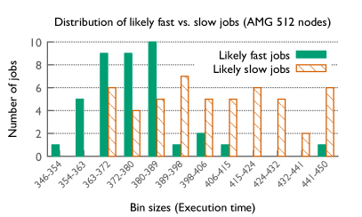
Figure 11: Distribution of actual runtimes of likely fast versus slow jobs of AMG when considering above median values of three features: RT_STL_COL, RT_STL_GBL, and NUM_GROUPS

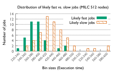
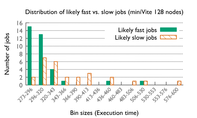
Figure 12: Distribution of actual runtimes of likely fast versus slow jobs of MILC and miniVite when considering above median values of three features: RT_STL_COL, RT_STL_GBL, and NUM_GROUPS

Once the jobs in a dataset have been classified into likely fast or slow based on the values of the selected network counters, we analyze their actual execution times to see if our classification is statistically significant. Figure 11 and 12 show the distributions of the execution times of the likely fast and slow sets of jobs in each application dataset. The histograms were generated with a fixed number of bins over the entire execution time range of a given dataset. Given the right skew present in application runtimes, we elected to use the Kruskal-Wallace H. Test to test for a difference in medians between the runtimes of likely fast and slow jobs in each application dataset. We found that for all the applications, the calculated p-value was below 3e-05, indicating a statistically significant difference between the likely fast and slow execution times. Note that a one-way ANOVA test yields statistically significant results below the 1% threshold for all applications. In all of the datasets analyzed here, we observe a statistically significant difference in the runtimes of the likely fast versus slow sets. Table IV compares the mean execution times of the likely fast versus slow jobs in each dataset. We can see that the difference is significant, especially for MILC and miniVite in spite of their predictions being poorer than AMG. This is a powerful result with significant implications for improving application performance and reducing variability.

TABLE IV: Mean execution times (in seconds) of the likely fast and slow subsets of jobs in each dataset

Application	Fast jobs	Slow jobs
AMG 128	260.12	274.24
AMG 512	379.93	410.68
MILC 128	317.31	398.43
MILC 512	389.61	445.80
miniVite 128	309.96	372.26

We foresee two immediate applications of such a system. When a job gets scheduled, individual HPC users can gather network counter data for a few minutes on all the routers assigned to their job and use our pre-trained models to predict the expected runtime of their application. They can use this prediction to decide if they should abort their job and resubmit or start running their program. Further, for stronger results, system administrators could pipe LDMS data into our system to provide instantaneous estimates of job performance through a command line tool. In either circumstance, resource sensitive users could decide whether to go ahead with launching their application or to give the allocation back and request another job.

Second, these results suggest that an intelligent job scheduler can monitor a handful of counters, and use their current values to determine if, for example, communication-heavy jobs will perform well or poorly if scheduled right away. Figures 11 and 12 demonstrate the power of predicting job execution time solely based on the median aggregation of just three network counters. While in this paper, we analyzed these jobs after they had run, a job scheduler would have access to similar counter data through LDMS at the time when a job is ready to be scheduled. Such adaptive decisions based on light-weight monitoring of a few hardware counters on a subset of routers would prove to be a useful tool.

VII Summary and Future Work

In this paper, we presented an data analytics study of longitudinal system-wide monitoring data to predict the performance of unseen jobs in the queue. We presented a pipeline for extracting relevant data from a time series, creating interpretable derived features, reducing the data, and filtering and aggregating it in meaningful ways. We then created several prediction models that only look at prior system state before a job starts executing to predict its runtime. Our models demonstrated good performance on two different metrics and also helped in identifying important input features.

We then demonstrated that using three network hardware counters and looking at their median values, we could classify jobs in a dataset into likely fast and likely slow with statistically significant results. This demonstrates that an intelligent job scheduler could use a similar simple mechanism or a more complex model-based approach to forecast the performance of a pending job. To the best of our knowledge, we believe that this is one of the first works that uses system-wide monitoring data and connects it with control experiments to predict the performance of unseen jobs.

In the future, we plan to investigate more detailed analysis of system monitoring data to detect patterns and anomalies in it. We also plan to create a large library of performance datasets that can be used to train machine learning models that would be successful in predicting performance of any new code. We also plan to improve job scheduling algorithms by incorporating machine learning models to make real-time decisions that reduce performance variability.

References

- [1] F. Petrini, D. J. Kerbyson, and S. Pakin, “The Case of the Missing Supercomputer Performance: Achieving Optimal Performance on the 8,192 Processors of ASCI Q,” in Proceedings of the 2003 ACM/IEEE conference on Supercomputing (SC’03), 2003.
- [2] A. Bhatele, K. Mohror, S. H. Langer, and K. E. Isaacs, “There goes the neighborhood: performance degradation due to nearby jobs,” in Proceedings of the ACM/IEEE International Conference for High Performance Computing, Networking, Storage and Analysis, ser. SC ’13. IEEE Computer Society, Nov. 2013. [Online]. Available: http://doi.acm.org/10.1145/2503210.2503247
- [3] A. Bhatele, J. J. Thiagarajan, T. Groves, R. Anirudh, S. A. Smith, B. Cook, and D. K. Lowenthal, “The case of performance variability on dragonfly-based systems,” in Proceedings of the IEEE International Parallel & Distributed Processing Symposium, ser. IPDPS ’20. IEEE Computer Society, May 2020 (to appear).
- [4] G. K. Lockwood, S. Snyder, T. Wang, S. Byna, P. Carns, and N. J. Wright, “A year in the life of a parallel file system,” in Proceedings of the International Conference for High Performance Computing, Networking, Storage, and Analysis, ser. SC ’18. IEEE Press, 2018.
- [5] J. Kim, W. J. Dally, S. Scott, and D. Abts, “Technology-driven, highly-scalable dragonfly topology,” in 2008 International Symposium on Computer Architecture. IEEE Computer Society, 2008.
- [6] A. Singh, “Load-balanced routing in interconnection networks,” Ph.D. dissertation, Dept. of Electrical Engineering, Stanford University, 2005, http://cva.stanford.edu/publications/2005/thesis_arjuns.pdf.
- [7] T. Groves, Y. Gu, and N. J. Wright, “Understanding performance variability on the aries dragonfly network,” in 2017 IEEE International Conference on Cluster Computing (CLUSTER), 2017, pp. 809–813.
- [8] T. Hoefler, T. Schneider, and A. Lumsdaine, “Characterizing the influence of system noise on large-scale applications by simulation,” in Proceedings of the 2010 ACM/IEEE International Conference for High Performance Computing, Networking, Storage and Analysis, ser. SC ’10. USA: IEEE Computer Society, 2010. [Online]. Available: https://doi.org/10.1109/SC.2010.12
- [9] O. Tuncer, E. Ates, Y. Zhang, A. Turk, J. Brandt, V. J. Leung, M. Egele, and A. K. Coskun, “Online diagnosis of performance variation in hpc systems using machine learning,” IEEE Transactions on Parallel and Distributed Systems, vol. 30, pp. 883–896, 2019.
- [10] A. Agelastos, B. Allan, J. Brandt, A. Gentile, S. Lefantzi, S. Monk, J. Ogden, M. Rajan, and J. Stevenson, “Continuous whole-system monitoring toward rapid understanding of production hpc applications and systems,” Parallel Computing, vol. 58, pp. 90 – 106, 2016. [Online]. Available: http://www.sciencedirect.com/science/article/pii/S0167819116300394
- [11] S. Chunduri, K. Harms, S. Parker, V. Morozov, S. Oshin, N. Cherukuri, and K. Kumaran, “Run-to-run variability on xeon phi based cray xc systems,” in Proceedings of the International Conference for High Performance Computing, Networking, Storage and Analysis, ser. SC ’17. New York, NY, USA: ACM, 2017.
- [12] S. Jha, J. Brandt, A. Gentile, Z. Kalbarczyk, and R. Iyer, “Characterizing supercomputer traffic networks through link-level analysis,” in 2018 IEEE International Conference on Cluster Computing (CLUSTER), Sep. 2018, pp. 562–570.
- [13] R. Wolski, N. Spring, and C. Peterson, “Implementing a performance forecasting system for metacomputing: The network weather service,” in Proceedings of the 1997 ACM/IEEE Conference on Supercomputing, ser. SC ’97. New York, NY, USA: Association for Computing Machinery, 1997. [Online]. Available: https://doi.org/10.1145/509593.509600
- [14] D. Skinner and W. Kramer, “Understanding the causes of performance variability in hpc workloads,” in Workload Characterization Symposium, 2005. Proceedings of the IEEE International. IEEE, 2005, pp. 137–149.
- [15] “Cori system.” [Online]. Available: https://docs.nersc.gov/systems/cori/
- [16] “Aries hardware counters (s-0045-20),” http://docs.cray.com/books/S-0045-20/S-0045-20.pdf, 2017.
- [17] R. Falgout, J. Jones, and U. Yang, “The design and implementation of hypre, a library of parallel high performance preconditioners,” in Numerical Solution of Partial Differential Equations on Parallel Computers, A. Bruaset and A. Tveito, Eds. Springer-Verlag, 2006, vol. 51, pp. 267–294.
- [18] S. Ghosh, M. Halappanavar, A. Tumeo, A. Kalyanaraman, H. Lu, D. Chavarrià-Miranda, A. Khan, and A. Gebremedhin, “Distributed louvain algorithm for graph community detection,” in 2018 IEEE International Parallel and Distributed Processing Symposium (IPDPS), May 2018, pp. 885–895.
- [19] S. Ghosh, M. Halappanavar, A. Tumeo, A. Kalyanaraman, and A. H. Gebremedhin, “Minivite: A graph analytics benchmarking tool for massively parallel systems,” in 2018 IEEE/ACM Performance Modeling, Benchmarking and Simulation of High Performance Computer Systems (PMBS), Nov 2018, pp. 51–56.
- [20] Y. Freund, R. Iyer, R. E. Schapire, and Y. Singer, “An efficient boosting algorithm for combining preferences,” Journal of machine learning research, vol. 4, no. Nov, pp. 933–969, 2003.
- [21] J. H. Friedman, “Greedy function approximation: A gradient boosting machine,” The Annals of Statistics, vol. 29, no. 5, pp. pp. 1189–1232, 2001.
- [22] N. Srivastava, “Improving neural networks with dropout,” University of Toronto, vol. 182, no. 566, p. 7, 2013.
- [23] P. Prettenhofer and G. Louppe, “Gradient boosted regression trees in scikit-learn,” 2014.
- [24] M. Sandri and P. Zuccolotto, “Analysis and correction of bias in total decrease in node impurity measures for tree-based algorithms,” Statistics and Computing, vol. 20, no. 4, pp. 393–407, 2010.