Four-frequency solution in a magnetohydrodynamic Couette flow as a consequence of azimuthal symmetry breaking

Abstract

The occurrence of magnetohydrodynamic (MHD) quasiperiodic flows with four fundamental frequencies in differentially rotating spherical geometry is understood in terms of a sequence of bifurcations breaking the azimuthal symmetry of the flow as the applied magnetic field strength is varied. These flows originate from unstable periodic and quasiperiodic states with broken equatorial symmetry but having four-fold azimuthal symmetry. A posterior bifurcation gives rise to two-fold symmetric quasiperiodic states, with three fundamental frequencies, and a further bifurcation to a four-frequency quasiperiodic state which has lost all the spatial symmetries. This bifurcation scenario may be favoured when differential rotation is increased and periodic flows with $m$-fold azimuthal symmetry, $m$ being product of several prime numbers, emerge at sufficiently large magnetic field.

Understanding how systems become chaotic is of fundamental importance in many applications. Biological systems Ermentrout (1985); Grigorov (2006), financial models Lorenz (1987), road traffic modelling Safonov et al. (2002), laser physics Hess et al. (1994), neural networks Albers and Sprott (2006), and simulations in fluid dynamics Castaño et al. (2016), or magnetohydrodynamics Garcia et al. (2020), exhibit transitions from regular oscillatory behaviour to a chaotic regime. Quite often, this transition follows the Newhouse-Ruelle-Takens (NRT) Newhouse et al. (1978) scenario in which after a few bifurcations, involving quasiperiodic states, chaos emerges. According to the NRT theorem quasiperiodic oscillatory motions, which are known as tori, with 3 or more fundamental frequencies are unstable to small perturbations and thus unlikely to occur. However, the numerical experiments of Grebogi et al. (1983) evidenced that the mathematical notion of small perturbations is a key issue and that in case of an appropriate spatial structure of the perturbations a three-tori solution may well be observed in real nonlinear systems. Since then, the existence of three-tori has been confirmed in experiments on electronic circuits Cumming and Linsay (1988); Sánchez et al. (2006), solid mechanics Alaggio and Rega (2000), hydrodynamics Langenberg et al. (2004), Rayleigh-Bénard convection Walden et al. (1984) and magnetohydrodynamics (MHD) Libchaber et al. (1983). The study of MHD flows is of fundamental relevance in geophysics and astrophysics which motivated experiments Stefani et al. (2006); Gailitis et al. (2002); Gallet et al. (2012); Stelzer et al. (2015) and simulations Roberts and Glatzmaier (2000); Jones (2011) that investigate the role of chaotic and/or turbulent flows for planetary and stellar dynamos Roberts and Stix (1971), or the turbulent transport processes occurring in accretion disks Balbus and Hawley (1998) where the magnetorotational instability (MRI) Balbus and Hawley (1991) plays a basic role.

Symmetries in physical systems provide a way to circumvent the NRT theorem because the bifurcations occurring in these systems may be non-generic. Their understanding is of relevance as the character of an underlying symmetry group in general is reflected in the possible solutions and their evolution in time, e.g. in terms of conservation laws. This is especially the case in fluid dynamics Crawford and Knobloch (1991), or magnetohydrodynamics, where the appearance of three-tori solutions has been interpreted as a consequence of bifurcations Lopez and Marques (2000); Libchaber et al. (1983), which may introduce a breaking of symmetry Altmeyer et al. (2012); Garcia et al. (2016, 2020). Quasiperiodic tori with more than three frequencies are however rarely found in systems with moderate and large number of degrees of freedom (e.g. Albers and Sprott (2006)). For instance, the existence of four-tori solutions has been attributed to the non-generic character of two-dimensional Rayleigh-Bénard convection Zienicke et al. (1998), or to spatial localisation of weakly coupled individual modes in Walden et al. (1984); He (2005). The latter studies pointed out the relevance of the spatial structure of the solutions for the emergence of chaos in large-scale systems.

In this Letter we investigate the emergence of four-tori and chaotic flows in simulations of a magnetised spherical Couette (MSC) system. Using an accurate frequency analysis based on Laskar’s algorithm Laskar (1993a) and Poincaré sections, we find that consecutive symmetry breaking caused by various Hopf bifurcations determine the evolution of the system and accompany the route to chaotic behaviour. The MSC system constitutes a paradigmatic MHD problem Hollerbach (2009); Travnikov et al. (2011); Figueroa et al. (2013); Wicht (2014) that is of relevance for differentially rotating, electrically conducting flows. Flows driven by differential rotation, which have been investigated in several experiments Sisan et al. (2004); Zimmerman et al. (2011); Hoff et al. (2016); Kasprzyk et al. (2017); Kaplan et al. (2018); Barik et al. (2018), govern the dynamics in the interior of stars and/or planets Jones (2011) where they constitute a possible source for MHD wave phenomena Spruit (2002), dynamo action , and perhaps even for the generation of gravitational wave signals from neutron stars Peralta et al. (2006); Lasky (2015).

In terms of symmetry theory Golubitsky and Stewart (2003) the MSC problem is a SO$(2)\times$Z₂ equivariant system, i.e., invariant by azimuthal rotations (SO$(2)$) and reflections with respect to the equatorial plane (Z₂). In SO$(2)$ symmetric systems, branches of rotating waves (RWs), either stable or unstable, appear after the axisymmetric base state becomes unstable (primary Hopf bifurcation Crawford and Knobloch (1991)). Successive Hopf bifurcations Rand (1982); Golubitsky et al. (2000) give rise to quasiperiodic modulated rotating waves (MRWs) and to chaotic turbulent flows, usually following the NRT scenario Rand (1982). In the particular case of the MSC, when the magnetic field is varied, branches of RWs with a $m$-fold azimuthal symmetry with a prime number $m=2,3$ Travnikov et al. (2011); Garcia and Stefani (2018) give rise to stable two- and three-tori MRWs Garcia et al. (2019), and eventually chaotic flows Garcia et al. (2020), though four-tori MRWs have not yet been found. We show below that MHD four-tori solutions in terms of MRWs can be obtained after successive azimuthal symmetry breaking Hopf bifurcations from a parent branch of RW having $m$-fold symmetry which is not a prime number, in this case $m=4$. Note that when $m$ is a prime number only one symmetry breaking bifurcation can take place as the flows are equatorially asymmetric so that the case $m=4$ constitutes the lowest non-trivial possibility for azimuthal symmetry breaking with multiple bifurcations.

We consider an electrically conducting fluid of density $\rho$, kinematic viscosity $\nu$, magnetic diffusivity $\eta=1/(\sigma\mu_{0})$ (where $\mu_{0}$ is the magnetic permeability of the free-space and $\sigma$ is the electrical conductivity). The fluid is bounded by two spheres with radius $r_{\text{i}}$ and $r_{\text{o}}$, respectively, with the outer sphere being at rest and the inner sphere rotating at angular velocity $\Omega$ around the vertical axis ${\bf\hat{e}_{z}}$ (see inset of Fig. 1). A uniform axial magnetic field of amplitude $B_{0}$ is imposed as in the HEDGEHOG experiment Kasprzyk et al. (2017). Scaling the length, time, velocity and magnetic field with $d=r_{\text{o}}-r_{\text{i}}$, $d^{2}/\nu$, $r_{\text{i}}\Omega$ and $B_{0}$, respectively, the temporal evolution of the system is governed by the Navier-Stokes equation and the induction equation which read:

$$\partial_{t}{\mathbf{v}}+{\rm Re}\left({\mathbf{v}}\cdot\nabla\right){\mathbf{v}}=-\nabla p+\nabla^{2}{\mathbf{v}}+{\rm Ha}^{2}(\nabla\times{\bf b})\times{\bf\hat{e}_{z}},$$

$$0=\nabla\times({\mathbf{v}}\times{\bf\hat{e}_{z}})+\nabla^{2}{\bf b},\quad\nabla\cdot{\mathbf{v}}=0,\quad\nabla\cdot{\bf b}=0,$$

where ${\rm Re}=\Omega r_{\text{i}}d/\nu$ is the commonly known Reynolds number, ${\rm Ha}=B_{0}d(\sigma/(\rho\nu))^{1/2}$ is the Hartmann number, ${\mathbf{v}}$ the velocity field and ${\bf b}$ the deviation of magnetic field from the axial applied field. Here we use the inductionless approximation which is valid in the limit of small magnetic Reynolds number, ${\rm Rm}=\Omega r_{\text{i}}d/\eta\ll 1$. This condition is well met when considering the liquid metal GaInSn, with magnetic Prandtl number ${\rm Pm}=\nu/\eta\sim O(10^{-6})$ Plevachuk et al. (2014), at moderate ${\rm Re}=10^{3}$ (similar to the experiment Kasprzyk et al. (2017)) since ${\rm Rm}={\rm Pm}\hskip 1.42262pt{\rm Re}\sim 10^{-3}$. The aspect ratio is $\chi=r_{\text{i}}/r_{\text{o}}=0.5$ and no-slip ($v_{r}=v_{\theta}=v_{\varphi}=0$) at $r=r_{\text{o}}$ and constant rotation ($v_{r}=v_{\theta}=0,~{}v_{\varphi}=\sin{\theta}$, $\theta$ being colatitude) at $r=r_{\text{i}}$ are the boundary conditions imposed on the velocity field. For the magnetic field, insulating boundary conditions are considered in accordance with typical experimental setups Sisan et al. (2004); Ogbonna et al. (2020). Spectral methods –spherical harmonics in the angular coordinates and a collocation method in the radial direction– and high order implicit-explicit backward-differentiation (IMEX–BDF) time schemes are employed for solving the MSC equations (see Garcia and Stefani (2018); Garcia et al. (2020) for details).

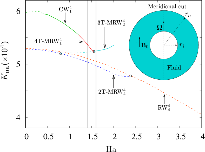
Figure 1: Magnetised spherical Couette (MSC) geometry and bifurcation diagram of the volume-averaged nonaxisymmetric kinetic energy density $K_{\text{na}}$ versus ${\rm Ha}$. Solid (dashed) lines are used for stable (unstable) flows. Branches of rotating waves RW${}^{m_{\text{max}}}_{m}$, modulated rotating waves MRW${}^{m_{\text{max}}}_{m}$, and complex waves CW${}^{m_{\text{max}}}_{m}$ are shown. MRWs with 2, 3 and 4 frequencies are labelled as 2T, 3T and 4T, respectively. The colours distinguish the various solutions according to the corresponding label. The vertical lines mark ${\rm Ha}$ for the solutions selected for Fig. 2.

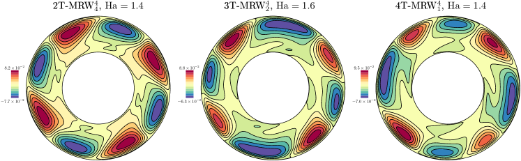
Figure 2: Contour plots of the nonaxisymmetric component of the radial velocity on a colatitudinal section at $\theta\approx 93^{\circ}$. The azimuthal symmetry is broken from left to right: from $m=4$ to $m=2$ and from $m=2$ to $m=1$ (compare the shape of the opposite red cells).

The solutions are classified according to their azimuthal symmetry $m$, the wave number with the largest volume-averaged kinetic energy $m_{\text{max}}$, and their type of time dependence. In this way, branches of RWs and MRWs are labelled as RW${}^{m_{\text{max}}}_{m}$ and MRW${}^{m_{\text{max}}}_{m}$. The latter can be quasiperiodic with 2, 3 and 4 frequencies and are labelled as 2T, 3T and 4T, respectively. The branches of equatorially asymmetric RW${}^{2}_{2}$, RW${}^{3}_{3}$, and RW${}^{4}_{4}$ which bifurcate from the base state at ${\rm Ha}=12.2$ Travnikov et al. (2011) were computed in Garcia and Stefani (2018) by means of continuation methods Doedel and Tuckerman (2000); Dijkstra et al. (2014); Sánchez and Net (2016). The latter allows, for each parameter, to find a periodic solution by applying a Newton method to a function derived from the flow periodicity condition (see Sánchez and Net (2016) for a detailed description). Here we focus on the analysis of MRW bifurcating from the unstable branch RW${}^{4}_{4}$ for a small control parameter ${\rm Ha}<2.5$ and fixed ${\rm Re}=10^{3}$. These MRWs have been successively obtained by means of direct numerical simulations (DNS) of the MSC equations with $n_{r}=40$ radial collocation points and a spherical harmonic truncation parameter of $L_{\text{max}}=84$. The dimension of the system is then $n=(2L_{\text{max}}^{2}+4L_{\text{max}})(n_{r}-1)=563472$. The results for the four-tori solution at ${\rm Ha}=1.4$ are confirmed for increased resolution with $n_{r}=60$ and $L_{\text{max}}=126$. Azimuthal symmetry $m=m_{d}$ can be imposed on the DNS by only considering the azimuthal wave numbers $m=km_{d},~{}k\in\mathbb{Z}$ in the spherical harmonic expansion of the fields. All DNS comprise more than 100 viscous time units and initial transients less than $10$ time units are required before the statistically saturated state is reached. The time and volume-averaged nonaxisymmetric kinetic energy density $K_{\text{na}}$ is employed as a proxy of the time dependence of the flows because they initially bifurcate from an axisymmetric base state (only the $m=0$ mode is nonzero). For each ${\rm Ha}$ a new MRW is computed from a previous state with nearby ${\rm Ha}$. We usually use $\Delta{\rm Ha}=0.1$, but smaller values are selected close to a bifurcation. The first branch of MRW which we compute here, bifurcates from the unstable branch RW${}^{4}_{4}$, already computed in Garcia and Stefani (2018).

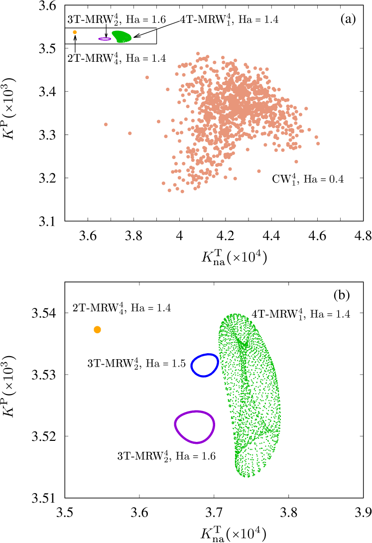
Figure 3: Poincaré sections at the time instants $t_{i}$ defined by the constraint $K(t_{i})=\overline{K}$, $K$ being the volume-averaged kinetic energy and $\overline{K}$ its time average. The volume-averaged poloidal kinetic energy $K^{\text{P}}(t_{i})$ is displayed versus the volume-averaged toroidal nonaxisymmetric energy $K^{\text{T}}_{\text{na}}(t_{i})$. (a) 2T-MRW${}^{4}_{4}$ at ${\rm Ha}=1.4$, 3T-MRW${}^{4}_{2}$ at ${\rm Ha}=1.6$, 4T-MRW${}^{4}_{1}$ at ${\rm Ha}=1.4$, and a chaotic wave CW${}^{4}_{1}$ at ${\rm Ha}=1.4$. (b) Detail of (a) showing also a 3T-MRW${}^{4}_{2}$ at ${\rm Ha}=1.5$.

The bifurcation diagram in Fig. 1 displays $K_{\text{na}}$ versus ${\rm Ha}$ and the bifurcation points are marked with circles. By decreasing ${\rm Ha}$, periodic RW${}^{4}_{4}$ undergo a Hopf bifurcation to 2T-MRW${}^{4}_{4}$ around ${\rm Ha}\approx 2.4$ which then extends down to ${\rm Ha}=0$. These flows are obtained with time integrations with the azimuthal symmetry constrained to $m=4$ and are unstable to small random perturbations with azimuthal symmetry $m=1$. Another branch of unstable solutions appears at ${\rm Ha}=0.8$ via a secondary subcritical Hopf bifurcation on the 2T-MRW${}^{4}_{4}$ branch (blue dashed curve) which breaks the $m=4$ symmetry to $m=2$ and finally leads to the emergence of an unstable 3T-MRW${}^{4}_{2}$ branch (light blue dashed curve). The latter extends for increasing ${\rm Ha}$ and becomes stable at ${\rm Ha}\approx 1.52$ where a branch of 4T-MRW${}^{4}_{1}$ is born thanks to a tertiary subcritical Hopf bifurcation breaking the $m=2$ symmetry (red curve). This branch is lost for ${\rm Ha}\lesssim 1.35$ (green curve) and complex flows, either with more than four frequencies or chaotic, occur. The contour plots of the $m\neq 0$ component of the radial velocity, on a colatitudinal section slightly below the equatorial plane, are displayed in Fig. 2 for one example of each type of MRW with azimuthal symmetry $m=4,m=2$, and $m=1$ (from left to right).

The time dependence of RWs is described by a uniform azimuthal rotation of a fixed flow pattern whereas for MRWs the pattern is azimuthally rotating but modulated with additional frequencies (e.g. Rand (1982)). Thus, a frequency analysis of any azimuthally averaged property provides one frequency less than the analysis of a localised particular flow component. Because of this, Poincaré sections at the time instants $t_{i}$ defined by the constraint $K(t_{i})=\overline{K}$, $K$ being the volume-averaged kinetic energy and $\overline{K}$ its time average, appear as a single point for 2T, a closed curve for 3T, a band of points for 4T, and a cloud of points for chaotic flows (Fig. 3). To confirm the regular behavior of 2T, 3T, and 4T MRWs we perform a frequency analysis. The frequencies giving rise to the modulation are accurately determined from the time series of $K_{4}$ ($K$ restricted to the $m=4$ mode) by means of a Fourier transform based optimisation algorithm by Laskar Laskar (1993a). If the solution is regular the frequencies do not depend (within the frequency determination accuracy) on the particular time window used for the analysis Laskar et al. (1992); Laskar (1993b). Sufficiently wide time windows ($5-40$ time units) over large time series ($100$ time units) are considered which leads to a relative accuracy around $10^{-5}$.

The power spectral density (psd) for $K_{4}$ is displayed in Fig. 4 for the same MRW as shown in Fig. 2 additionally including the psd for a chaotic solution at ${\rm Ha}=0.4$ (bottom curve). Some examples for the fundamental frequencies or corresponding linear combinations $\sum k_{i}f_{i}$ with $k_{i}$ being integers, are explicitly marked. In all cases we have checked that the relative accuracy $|f-\sum k_{i}f_{i}|/f<10^{-5}$, with $-6\leq k_{i}\leq 6$, for all frequencies obtained with Laskar’s algorithm. In the simplest case, the 2T-MRW${}_{4}^{4}$ at ${\rm Ha}=1.4$, only one fundamental frequency $f_{1}$ and its multiples are present, because the fundamental frequency associated to the drift motion is removed by volume averaging. A second frequency $f_{2}$ and few combinations $k_{1}f_{1}+k_{2}f_{2}$ occur for the 3T-MRW${}^{4}_{2}$ whereas the psd of 4T-MRW${}^{4}_{1}$ reveals a complex time dependence with several combinations of the type $k_{1}f_{1}+k_{2}f_{2}+k_{3}f_{3}$. For ${\rm Ha}\lesssim 1.35$ the variation of the main frequency $f_{1}$ becomes larger than the accuracy and thus 4T-MRW${}^{4}_{1}$ give rise to more complex motions, which could be regular flows with a very small additional frequency or chaotic flows. However, deciding whether a new very small frequency has appeared in this regime would require extremely long time integrations of the MSC system, which are out of the scope of the present study. Nevertheless, it is clear that fully broadband frequency distribution characteristic for chaotic flows is obtained for ${\rm Ha}\lesssim 0.7$. The psd for the chaotic solution at ${\rm Ha}=0.4$ shown in Fig. 4 (bottom curve) exhibits a noticeable peak that corresponds to the main frequency of modulation of the original MRW.

As suggested in Walden et al. (1984), the strong polar localisation of the $m=1$ (also $m=3$) perturbations (see Fig. 1, supplementary material) provides a way to overcome the NRT requirements and thus explains the existence of 4T-MRW${}^{4}_{1}$. In our case, successive azimuthal symmetry breaking bifurcations from unstable regular states (that can not be realised in the experiments of Walden et al. (1984)) are responsible for the mode localisation. For the regular solutions, the kinetic energy fluctuations of the different modes evidence a weak nonlinear interaction, being the $m=4$ component which most contributes to the flow (see Figure 2 supplementary material, also the kinetic energy spectra in Fig. 5). The amplitude of fluctuations leading to chaotic flows seem not to be associated to turbulent spatial behaviour as the $m=4$ component of the flow still dominates over the other modes (Fig. 5).

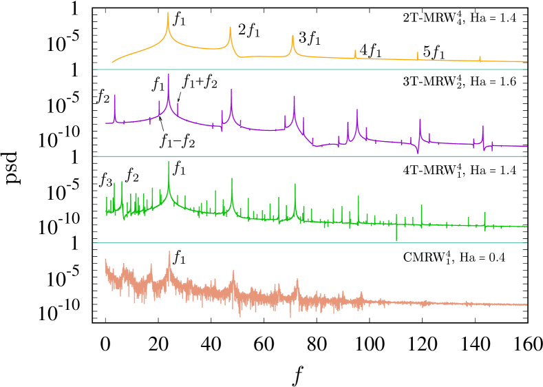
Figure 4: Power spectral density for the volume-averaged kinetic energy density $K_{4}$ of the $m=4$ mode for 2T-MRW${}^{4}_{4}$ at ${\rm Ha}=1.4$, 3T-MRW${}^{4}_{2}$ at ${\rm Ha}=1.6$, 4T-MRW${}^{4}_{1}$ at ${\rm Ha}=1.4$, and a chaotic wave CW${}^{4}_{1}$ at ${\rm Ha}=1.4$. The time series of $K_{4}$ are displayed on Fig. 2 of the supplementary material.

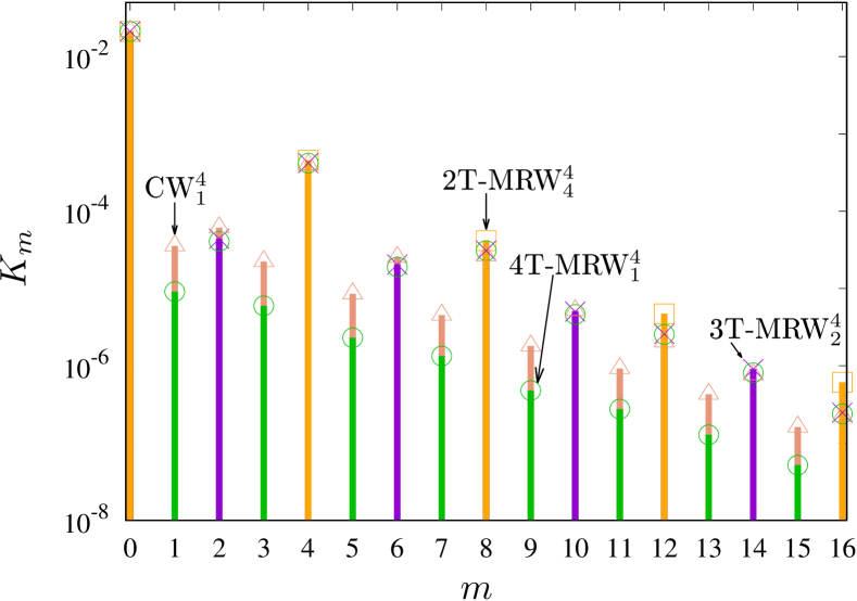
Figure 5: (a) Kinetic energy spectra ($K_{m}$ versus $m$) for 2T-MRW${}^{4}_{4}$ at ${\rm Ha}=1.4$ ($\square$), 3T-MRW${}^{4}_{2}$ at ${\rm Ha}=1.6$ ($\times$), 4T-MRW${}^{4}_{1}$ at ${\rm Ha}=1.4$ ($\circ$), and a chaotic flow CW${}^{4}_{1}$ at ${\rm Ha}=0.4$ ($\bigtriangleup$).

The present study evidences that four-tori solutions are physically possible in MHD problems and can be explained in terms of bifurcation theory. The bifurcation scenario resembles the NRT scenario but involves two additional Hopf bifurcations, including a subcritical bifurcation leading to a stabilisation of a three-tori solution. This kind of stabilisation was also found in Mamun and Tuckerman (1995), but for axisymmetric steady states, arising in purely hydrodynamic spherical Couette (SC) flows. Further SC experiments Wulf et al. (1999) are in accordance with the NRT scenario, but only two-tori were detected before the regime of chaotic flows. Similarly, three or four-tori have not been found in a comprehensive study of the different flow regimes in the SC system with positive or negative differential rotation Wicht (2014). When the magnetic field is included, several MSC regimes have been studied recently Hollerbach (2009); Gissinger et al. (2011); Kaplan et al. (2018) but the existence of quasiperiodic flows with three frequencies has not been shown until Garcia et al. (2020).

The fundamental result presented here is that in a system with symmetry, more symmetry breaking bifurcations may be required in the NRT scenario until a flow can become chaotic, and thus regular motions with three or four frequencies are likely to occur, formed by modes localised in different parts of the domain Walden et al. (1984). These flows originate from unstable states of azimuthal symmetry $m=4$ and thus their origin can only be understood with symmetrically constrained simulations and not with experiments. Speculatively, periodic flows with an azimuthal symmetry that constitute a product of several prime numbers, may give rise to quasiperiodic flows with more than four frequencies, as several symmetry breaking bifurcations can occur. The new frequency occurring at the bifurcation is usually smaller (but also can be larger, e. g. Walden et al. (1984)) than the previous fundamental one, as can be seen in Fig. 4. With on going bifurcations the effect requires a longer time evolution of the system until the upcoming frequency can be detected in the captured time series. The smallest fundamental frequency of the simulated 4T-MRW${}^{4}_{1}$ at ${\rm Ha}=1.4$ gives rise to a time scale of around 1600 seconds which should be detectable in the HEDGEHOG experiment Kasprzyk et al. (2017), whose duration is limited to 10 hours due to the decrease of signal quality of flow measurement Ogbonna et al. (2020). The results also bear relevance for the MRI as previous experiments Sisan et al. (2004) may be understood in terms of MSC instabilities Hollerbach (2009); Gissinger et al. (2011), similar to those analysed here.

I Supplementary material

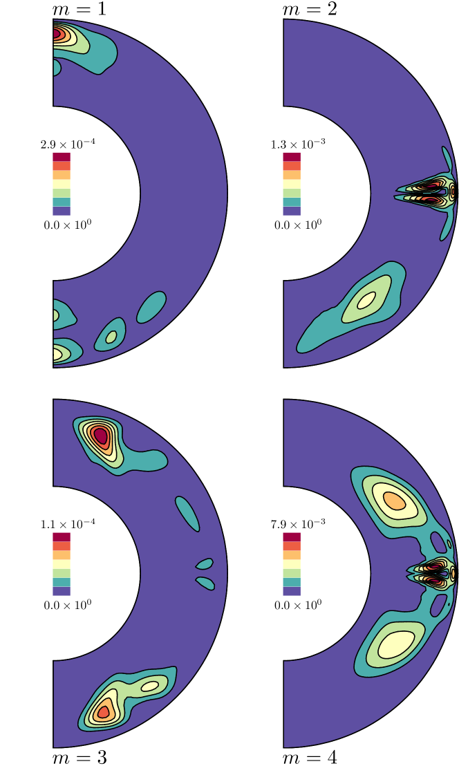
Figure 6: Contour plots of the $m=1,2,3,4$ components (from left to right and from top to bottom) of the kinetic energy density on a meridional section through a relative maximum. The solution is the 4T-MRW${}^{4}_{1}$ at ${\rm Ha}=1.4$ displayed on the rightmost plot of Fig. 2 of the main manuscript.

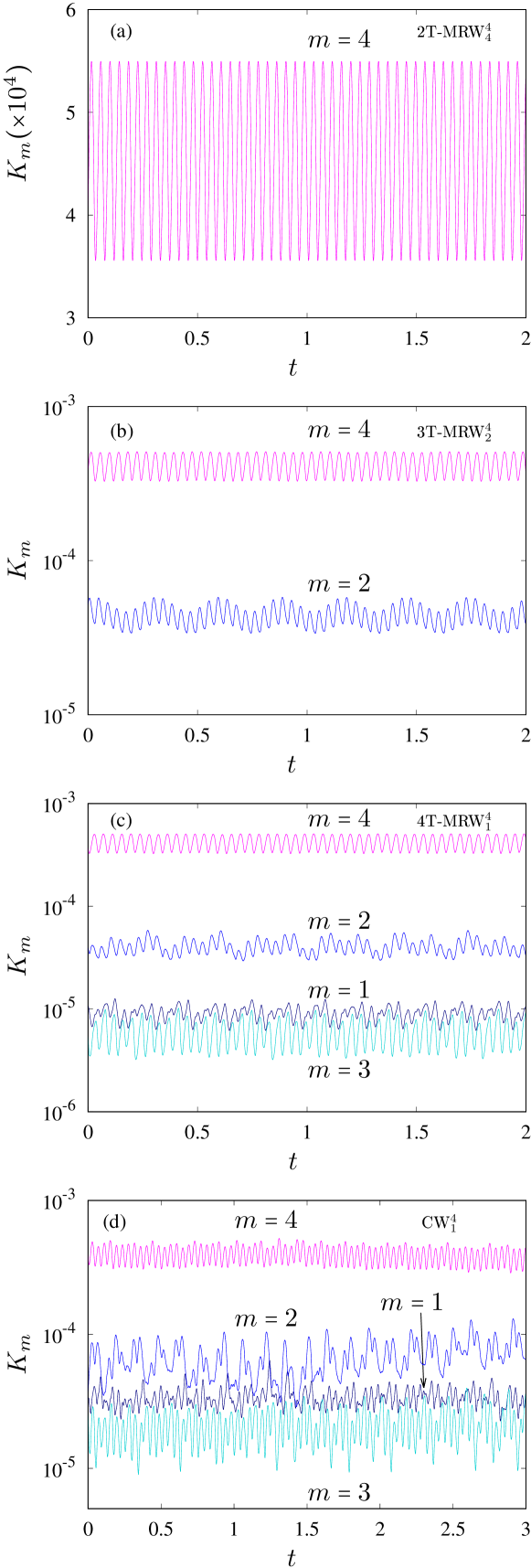
Figure 7: Time series of the volume-averaged kinetic energy contained in each azimuthal wave number $m=1,2,3,4$. (a) Two frequency solution 2T-MRW${}^{4}_{4}$ at ${\rm Ha}=1.4$. Only the modes $m=4k,~{}k\in\mathbb{Z}$ are nonzero. (b) Three frequency solution 3T-MRW${}^{4}_{2}$ at ${\rm Ha}=1.6$. Only the modes $m=2k,~{}k\in\mathbb{Z}$ are nonzero. (c) Four frequency solution 4T-MRW${}^{4}_{1}$ at ${\rm Ha}=1.4$. All the modes $m\in\mathbb{Z}$ are nonzero. (d) Chaotic solution at ${\rm Ha}=0.4$. Panels (a),(b) and (c) correspond to the contour plots, from left to right respectively, shown in figure 2 of the main manuscript. The power spectral density of the time series corresponding to $K_{4}$ are displayed on figure 4 of the main manuscript.

The modulated rotating waves (MRWs) presented in the main manuscript have been successively obtained by means of direct numerical simulations (DNS) of the magnetised spherical Couette (MSC) equations with $n_{r}=40$ radial collocation points and a spherical harmonic truncation parameter of $L_{\text{max}}=84$. The dimension of the system is then $n=(2L_{\text{max}}^{2}+4L_{\text{max}})(n_{r}-1)=563472$. The results for the four-tori solution at ${\rm Ha}=1.4$ are confirmed for increased resolution with $n_{r}=60$ and $L_{\text{max}}=126$. Azimuthal symmetry $m=m_{d}$ can be imposed on the DNS by only considering the azimuthal wave numbers $m=km_{d},~{}k\in\mathbb{Z}$ in the spherical harmonic expansion of the fields. All DNS comprise more than 100 viscous time units and initial transients less than $10$ time units are required before the statistically saturated state is reached. For each ${\rm Ha}$ a new MRW is computed from a previous state with nearby ${\rm Ha}$. We usually use $\Delta{\rm Ha}=0.1$, but smaller values are selected close to a bifurcation. The first branch of MRW which we compute in the present study, bifurcates from the unstable branch RW${}^{4}_{4}$, already computed in Garcia and Stefani (2018).

Figure 6 corresponds to the 4T-MRW${}^{4}_{1}$ at ${\rm Ha}=1.4$ and displays, from left to right and from top to bottom, the contour plots of the kinetic energy density, on a meridional section through a relative maxima, for the $m=1$, $m=2$, $m=3$ and $m=4$ modes, respectively. While fluid motions remain confined to mid and low latitudes in the case of $m=2$ and $m=4$ modes (even modes), the flow is restricted to high latitudes in the case of odd modes ($m=1$ and $m=3$). Then, even modes contribute to motions outside the tangent cylinder (an imaginary cylinder parallel to the rotation axis and tangent to the inner sphere) whereas odd modes contribute to motions within the tangent cylinder. As suggested in Walden et al. (1984) the different localisation of the different modes within the domain may explain the appearance of flows with four fundamental frequencies.

To describe the nature of kinetic energy fluctuations, the time series of the volume-averaged kinetic energy of each azimuthal wave number $m=1,2,3,4$ is displayed in figure 7(a-c) for the three types of MRW shown in Figs. 2,4 and 5 of the main manuscript: A 2T-MRW${}^{4}_{4}$, a 3T-MRW${}^{4}_{2}$, and a 4T-MRW${}^{4}_{1}$. The dominance of the $m=4$ component of the flow and the quasiperiodic character of the waves are clear from the figure. The modes arising at the symmetry breaking bifurcations ($m=1,2,3$) have larger fluctuations than the main $m=4$ component of the flow, but barely contribute to the total kinetic energy. The time series for a chaotic solution CW${}^{4}_{1}$ is plotted in Fig. 7(d) and shows a larger contribution of the non-dominant $m=1,2,3$ modes.

F. G. was supported by the Alexander von Humboldt Foundation. This project has also received funding from the European Research Council (ERC) under the European Union’s Horizon 2020 research and innovation programme (grant agreement No 787544).

References

- Ermentrout (1985) G. B. Ermentrout, “The behavior of rings of coupled oscillators,” J. Math. Biol. 23, 55–74 (1985).
- Grigorov (2006) M. G. Grigorov, “Global dynamics of biological systems from time-resolved omics experiments,” Bioinformatics 22, 1424–1430 (2006).
- Lorenz (1987) H.-W. Lorenz, “Strange attractors in a multisector business cycle model,” J. Econ. Behav. Organ. 8, 397 – 411 (1987).
- Safonov et al. (2002) L. A. Safonov, E. Tomer, V. V. Strygin, Y. Ashkenazy, and S. Havlin, “Multifractal chaotic attractors in a system of delay-differential equations modeling road traffic,” CHAOS 12, 1006–1014 (2002).
- Hess et al. (1994) O. Hess, D. Merbach, H.-P. Herzel, and E. Scholl, “Bifurcations of a three-torus in a twin-stripe semiconductor laser model,” Phys. Lett. A 194, 289 – 294 (1994).
- Albers and Sprott (2006) D.J. Albers and J.C. Sprott, “Routes to chaos in high-dimensional dynamical systems: A qualitative numerical study,” Physica D 223, 194–207 (2006).
- Castaño et al. (2016) D. Castaño, M. C. Navarro, and H. Herrero, “Evolution of secondary whirls in thermoconvective vortices: Strengthening, weakening, and disappearance in the route to chaos,” Phys. Rev. E 93, 013117 (2016).
- Garcia et al. (2020) F. Garcia, M. Seilmayer, A. Giesecke, and F. Stefani, “Chaotic wave dynamics in weakly magnetised spherical Couette flows,” CHAOS 30, 043116 (2020).
- Newhouse et al. (1978) S. Newhouse, D. Ruelle, and F. Takens, “Occurrence of strange axiom A attractors near quasiperiodic flows on , ,” Commun. Math. Phys. 64, 35–40 (1978).
- Grebogi et al. (1983) C. Grebogi, E. Ott, and J. A. Yorke, “Are three-frequency quasiperiodic orbits to be expected in typical nonlinear dynamical systems?” Phys. Rev. Lett. 51, 339–342 (1983).
- Cumming and Linsay (1988) A. Cumming and P. S. Linsay, “Quasiperiodicity and chaos in a system with three competing frequencies,” Phys. Rev. Lett. 60, 2719–2722 (1988).
- Sánchez et al. (2006) E. Sánchez, D. Pazó, and M. A. Matías, “Experimental study of the transitions between synchronous chaos and a periodic rotating wave,” CHAOS 16, 033122 (2006).
- Alaggio and Rega (2000) R. Alaggio and G. Rega, “Characterizing bifurcations and classes of motion in the transition to chaos through 3D-tori of a continuous experimental system in solid mechanics,” Physica D 137, 70–93 (2000).
- Langenberg et al. (2004) J. Langenberg, G. Pfister, and J. Abshagen, “Chaos from Hopf bifurcation in a fluid flow experiment,” Phys. Rev. E 70, 046209 (2004).
- Walden et al. (1984) R. W. Walden, P. Kolodner, A. Passner, and C. M. Surko, “Nonchaotic rayleigh-bénard convection with four and five incommensurate frequencies,” Phys. Rev. Lett. 53, 242–245 (1984).
- Libchaber et al. (1983) A. Libchaber, S. Fauvé, and C. Laroche, “Two-parameter study of the routes to chaos,” Physica D 7, 73 – 84 (1983).
- Stefani et al. (2006) F. Stefani, T. Gundrum, G. Gerbeth, G. Rüdiger, M. Schultz, J. Szklarski, and R. Hollerbach, “Experimental evidence for magnetorotational instability in a Taylor-Couette flow under the influence of a helical magnetic field,” Phys. Rev. Lett. 97, 184502 (2006).
- Gailitis et al. (2002) A. Gailitis, O. Lielausis, E. Platacis, G Gerbeth, and F. Stefani, “Colloquium: Laboratory experiments on hydromagnetic dynamos,” Rev. Modern Phys. 74, 973–990 (2002).
- Gallet et al. (2012) B. Gallet, S. Aumaître, J. Boisson, F. Daviaud, B. Dubrulle, N. Bonnefoy, M. Bourgoin, Ph. Odier, J.-F. Pinton, N. Plihon, G. Verhille, S. Fauve, and F. Pétrélis, “Experimental observation of spatially localized dynamo magnetic fields,” Phys. Rev. Lett. 108, 144501 (2012).
- Stelzer et al. (2015) Z. Stelzer, S. Miralles, D. Cébron, J. Noir, S. Vantieghem, and A. Jackson, “Experimental and numerical study of electrically driven magnetohydrodynamic flow in a modified cylindrical annulus. II. Instabilities,” Phys. Fluids 27, 084108 (2015).
- Roberts and Glatzmaier (2000) P. H. Roberts and G. A. Glatzmaier, “Geodynamo theory and simulations,” Rev. Modern Phys. 72, 1081–1123 (2000).
- Jones (2011) C. A. Jones, “Planetary magnetic fields and fluid dynamos,” Ann. Rev. Fluid Mech. 43, 583–614 (2011).
- Roberts and Stix (1971) P. H. Roberts and M. Stix, “The turbulent dynamo: A translation of a series of papers by F. Krause, K.-H Radler, and M. Steenbeck,” NCAR Technical Notes Collection TN-60+IA (1971).
- Balbus and Hawley (1998) S. A. Balbus and J. F. Hawley, “Instability, turbulence, and enhanced transport in accretion disks,” Rev. Modern Phys. 70, 1–53 (1998).
- Balbus and Hawley (1991) S. A. Balbus and J. F. Hawley, “A powerful local shear instability in weakly magnetized disks. i- Linear analysis. ii- Nonlinear evolution,” Astrophys. J. 376, 214–233 (1991).
- Crawford and Knobloch (1991) J. D. Crawford and E. Knobloch, “Symmetry and symmetry-breaking bifurcations in fluid dynamics,” Ann. Rev. Fluid Mech. 23, 341–387 (1991).
- Lopez and Marques (2000) J. M. Lopez and F. Marques, “Dynamics of three-tori in a periodically forced Navier-Stokes flow,” Phys. Rev. Lett. 85, 972–975 (2000).
- Altmeyer et al. (2012) S. Altmeyer, Y. Do, F. Marques, and J. M. Lopez, “Symmetry-breaking Hopf bifurcations to 1-, 2-, and 3-tori in small-aspect-ratio counterrotating Taylor-Couette flow,” Phys. Rev. E 86, 046316 (2012).
- Garcia et al. (2016) F. Garcia, M. Net, and J. Sánchez, “Continuation and stability of convective modulated rotating waves in spherical shells,” Phys. Rev. E 93, 013119 (2016).
- Zienicke et al. (1998) E. Zienicke, N. Seehafer, and F. Feudel, “Bifurcations in two-dimensional Rayleigh-Bénard convection,” Phys. Rev. E 57, 428–435 (1998).
- He (2005) K. He, “Riddling of the orbit in a high dimensional torus and intermittent energy bursts in a nonlinear wave system,” Phys. Rev. Lett. 94, 034101 (2005).
- Laskar (1993a) J. Laskar, “Frequency analysis of a dynamical system,” Celestial Mech. Dyn. Astr. 56, 191–196 (1993a).
- Hollerbach (2009) R. Hollerbach, “Non-axisymmetric instabilities in magnetic spherical Couette flow,” Proc. Roy. Soc. Lond. A 465, 2003–2013 (2009).
- Travnikov et al. (2011) V. Travnikov, K. Eckert, and S. Odenbach, “Influence of an axial magnetic field on the stability of spherical Couette flows with different gap widths,” Acta Mech. 219, 255–268 (2011).
- Figueroa et al. (2013) A. Figueroa, N. Schaeffer, H.-C. Nataf, and D. Schmitt, “Modes and instabilities in magnetized spherical Couette flow,” J. Fluid Mech. 716, 445–469 (2013).
- Wicht (2014) Johannes Wicht, “Flow instabilities in the wide-gap spherical Couette system,” J. Fluid Mech. 738, 184–221 (2014).
- Sisan et al. (2004) D. R. Sisan, N. Mujica, W. A. Tillotson, Y. M. Huang, W. Dorland, A. B. Hassam, T. M. Antonsen, and D. P. Lathrop, “Experimental observation and characterization of the magnetorotational instability,” Phys. Rev. Lett. 93, 114502 (2004).
- Zimmerman et al. (2011) D. S. Zimmerman, S. A. Triana, and D. P. Lathrop, “Bi-stability in turbulent, rotating spherical Couette flow,” Phys. Fluids 23, 065104 (2011).
- Hoff et al. (2016) M. Hoff, U. Harlander, and C. Egbers, “Experimental survey of linear and nonlinear inertial waves and wave instabilities in a spherical shell,” J. Fluid Mech. 789, 589–616 (2016).
- Kasprzyk et al. (2017) C. Kasprzyk, E. Kaplan, M. Seilmayer, and F. Stefani, “Transitions in a magnetized quasi-laminar spherical Couette flow,” Magnetohydrodynamics 53, 393–401 (2017).
- Kaplan et al. (2018) E. J. Kaplan, H.-C. Nataf, and N. Schaeffer, “Dynamic domains of the Derviche Tourneur sodium experiment: Simulations of a spherical magnetized Couette flow,” Phys. Rev. Fluids 3, 034608 (2018).
- Barik et al. (2018) A. Barik, S. A. Triana, M. Hoff, and J. Wicht, “Triadic resonances in the wide-gap spherical Couette system,” J. Fluid Mech. 843, 211–243 (2018).
- Spruit (2002) H. C. Spruit, “Dynamo action by differential rotation in a stably stratified stellar interior,” Astron. & Astrophys. 381, 923–932 (2002).
- Note (1) A differentially rotating flow, for example, provides a natural explanation for the strong axisymmetric character of Saturn’s magnetic field Wicht and Olson (2010).
- Peralta et al. (2006) C. Peralta, A. Melatos, M. Giacobello, and A. Ooi, “Gravitational radiation from nonaxisymmetric spherical Couette flow in a neutron star,” Astrophys. J. Lett. 644, L53–L56 (2006).
- Lasky (2015) P. D. Lasky, “Gravitational Waves from Neutron Stars: A Review,” Publications of the Astronomical Society of Australia 32, e034 (2015).
- Golubitsky and Stewart (2003) M. Golubitsky and I. Stewart, The symmetry perspective: From equilibrium to chaos in phase space and physical space. (Birkhäuser, Basel, 2003).
- Rand (1982) D. Rand, “Dynamics and symmetry. Predictions for modulated waves in rotating fluids,” Arch. Ration. Mech. An. 79, 1–37 (1982).
- Golubitsky et al. (2000) M. Golubitsky, V. G. LeBlanc, and I. Melbourne, “Hopf bifurcation from rotating waves and patterns in physical space,” J. Nonlinear Sci. 10, 69–101 (2000).
- Garcia and Stefani (2018) F. Garcia and F. Stefani, “Continuation and stability of rotating waves in the magnetized spherical Couette system: Secondary transitions and multistability,” Proc. Roy. Soc. Lond. A 474, 20180281 (2018).
- Garcia et al. (2019) F. Garcia, M. Seilmayer, A. Giesecke, and F. Stefani, “Modulated rotating waves in the magnetized spherical Couette system,” J. Nonlinear Sci. 29, 2735–2759 (2019).
- Plevachuk et al. (2014) Y. Plevachuk, V. Sklyarchuk, S. Eckert, G. Gerbeth, and R. Novakovic, “Thermophysical properties of the liquid Ga-In-Sn eutectic alloy,” J. Chem. Eng. Data 59, 757–763 (2014).
- Ogbonna et al. (2020) J. Ogbonna, F. Garcia, T. Gundrum, M. Seilmayer, and F. Stefani, “Experimental investigation of the return flow instability in magnetic spherical Couette flow,” (2020), submitted to Phys. Fluids., arXiv:2009.07003 [physics.flu-dyn] .
- Doedel and Tuckerman (2000) E. Doedel and L. S. Tuckerman, eds., Numerical Methods for Bifurcation Problems and Large-Scale Dynamical Systems, IMA Volumes in Mathematics and its Applications, Vol. 119 (Springer–Verlag, Berlin, 2000).
- Dijkstra et al. (2014) H. A. Dijkstra, F. W. Wubs, A. K. Cliffe, E. Doedel, I. F. Dragomirescu, B. Eckhardt, A. Y. Gelfat, A. L. Hazel, V. Lucarini, A. G. Salinger, E. T. Phipps, J. Sánchez-Umbría, H. Schuttelaars, L. S. Tuckerman, and U. Thiele, “Numerical bifurcation methods and their application to fluid dynamics: Analysis beyond simulation,” Commun. Comput. Phys. 15, 1–45 (2014).
- Sánchez and Net (2016) J. Sánchez and M. Net, “Numerical continuation methods for large-scale dissipative dynamical systems,” Eur. Phys. J. Spec. Top. 225, 2465–2486 (2016).
- Laskar et al. (1992) J. Laskar, C. Froeschlé, and A. Celletti, “The measure of chaos by the numerical analysis of the fundamental frequencies. application to the standard mapping,” Physica D 56, 253 – 269 (1992).
- Laskar (1993b) J. Laskar, “Frequency analysis for multi-dimensional systems. Global dynamics and diffusion,” Physica D 67, 257–281 (1993b).
- Mamun and Tuckerman (1995) C. K. Mamun and L. S. Tuckerman, “Asymmetry and Hopf bifurcation in spherical Couette flow,” Phys. Fluids 7, 80–91 (1995).
- Wulf et al. (1999) P. Wulf, C. Egbers, and H. J. Rath, “Routes to chaos in wide-gap spherical Couette flow,” Phys. Fluids 11, 1359–1372 (1999).
- Gissinger et al. (2011) C. Gissinger, H. Ji, and J. Goodman, “Instabilities in magnetized spherical Couette flow,” Phys. Rev. E 84, 026308 (2011).
- Wicht and Olson (2010) J. Wicht and P. Olson, “Differential rotation dynamos: An application to Saturn,” in Geophysical Research Abstracts (EGU General Assembly, 2010) p. 10179.