Off-grid Multi-Source Passive Localization Using a Moving Array

Abstract

A novel direct passive localization technique through a single moving array is proposed in this paper using the sparse representation of the array covariance matrix in spatial domain. The measurement is constructed by stacking the vectorized version of all the array covariance matrices at different observing positions. First, an on-grid compressive sensing (CS) based method is developed, where the dictionary is composed of the steering vectors from the searching grids to the observing positions. Convex optimization is applied to solve the ${\ell_{1}}$-norm minimization problem. Second, to get much finer target positions, we develop an on-grid CS based method, where the majorization-minimization technique replaces the atan-sum objective function in each iteration by a quadratic convex function which can be easily minimized. The objective function, atan-sum, is more similar to ${\ell_{0}}$-norm, and more sparsity encouraging than the log-sum function. This method also works more robustly at conditions of low SNR, and fewer observing positions are needed than in the traditional ones. The simulation experiments verify the promises of the proposed algorithm.

1 Introduction

Finding the positions of passive sources from an array of spatially separated sensors has been of considerable interest for decades in both military and civilian applications, such as radar, sonar, and global positioning systems, mobile communications, multimedia, and wireless sensor networks.

There is a vast literature dedicated to the passive localization problem applying classical signal-processing methods. The measurements needed for the localization problem are usually the phase, strength, or time information of the signals impinging on the antennas. Thus, the localization techniques are often based on the time of arrival (TOA), time difference of arrival (TDOA), received signal strength (RSS), direction of arrival (DOA) [1] [2], and phase difference rate [3] of the intercepted signals.

The bearing only localization (BOL) or the phase difference rate based algorithms essentially make use of the phase difference information of the signals. The sensors are often modeled as a narrow bandwidth receiving antenna array. In the traditional ways, the position of the target is obtained using a two-step method. First, the DOA of the target is estimated using multiple signal classification (MUSIC) or the phase differences.Second, the position of the target is estimated using those multiple measurements of the DOA or the phase difference rates. However, this two-step localization approach suffers from the nonlinear relationships between the phase difference and the target position. It also has poor signal-to-noise ratio (SNR) performance.

Furthermore, the localization researches usually simply deal with the single-target problems traditionally. The multiple-target- localization problem should be divided into multiple single-target-localization problems only if the measurement can be uniquely assigned to individual targets. A one-step localization for multiple sources are proposed in [4] by communicating the estimated covariance matrix between decentralized sub-arrays, which processing only increases the load of the communication slightly. This is a MUSIC like algorithm based on subspace decomposition. It has the ability of positioning multiple targets simultaneously. Same idea is used in [5] for a moving array localization problem, where a Cramér-Rao Bound (CRB) is given. Along with the development of compressive sensing (CS), a joint sparse representation of array covariance matrices (JSRACM) for emitter locations on multiple phase arrays is proposed in [6]. The locations may be estimated by solving an unconstrained optimization problem.

1.1 Compressed sensing and Location problems

Compressed sensing which is also called sparse recovery has witnessed an increasing interest in recent years to meet the high demand for efficient information acquisition scheme [7]. Contrary to the traditional Nyquist criteria, CS, depending on finding sparse solutions to underdetermined linear systems, can reconstruct the signals from far fewer samples than is possible using Nyquist sampling rate. CS has seen major applications in diverse fields, ranging from image processing to array signal processing. These applications have been successful because of the inherent sparsity of many real-world signals like sound, image, and video.

The early works in CS assume the sparse solutions lie on some fixed grids. However, this is not true in practical applications, so off-grid CS is proposed. In off-grid scenarios, an atomic norm minimization approach is proposed in [8] to exactly recover the unknown waveform. The problem is solved by reformulating it as an exact semidefinite program. In [9], atomic norms are further studied in the line spectral estimation in a noisy condition. Alternatively, an iterative reweighted method for off-grid CS is proposed in [10], where the sparse signals and the unknown parameters used to construct the true dictionary are jointly estimated.

As soon as the concept of the off-grid CS emerged, it was quickly applied to DOA and localization problems. In [11], joint sparsity reconstruction methods is used to estimate the DOA by exploring the underlying structure between the sparse signal and the gird mismatch for off-grid targets. The idea is to approximate the measurement matrix by using the first order Taylor expansion around the predefined grid. Atomic norm based off-grid CS is used to the same DOA problem in [12], which achieves high-resolution DOA estimation through the polynomial rooting method. The counting and localization problem for off-grid targets in wireless sensor networks is also formulated to a sparse recovery problem [13], where the true and unknown sparsifying dictionary is approximated with its first order Taylor expansion around a known dictionary. To locate multiple sources through TDOA measurements, [14] proposes a new Bayesian learning method for cases where the off-grid error is considered.

1.2 The main contribution of this paper

In this paper, we propose a novel localization algorithm and its theoretical analysis which is designed for multi-source passive localization. To summarize, the main contribution of this paper is as follows,

i. By the array covariance matrix based on off-grid CS, a novel sparse recovery algorithm which has the ability of estimating multiple targets positions simultaneously. A better localization performance can be achieved by fewer antenna elements and fewer observing positions compared to the traditional BOL methods.

ii. Due to the difficult caused by $\ell_{0}$-minimization, we use arc-tangent function to replace the original $0$-norm. In order to ensure that both the NP-HARD original model and the continuous alternative optimization model share the same sparse solution, we prove the equivalence between these two models which can explain the reason theoretically why the proposed method performs better than classic methods.

In the proposed method, the measurement of the localization formulation is obtained by stacking all the estimated array covariance matrices from different observing positions together. To begin with, an on-grid localization is achieved simply by sparsely representing the intercepted signals in the spatial domain with an over-complete basis. Convex optimization is then used to solve the constrained ${\ell_{1}}$-norm minimization problem.

However, to get a more precise target position, much finer grids are needed, such that the size of the dictionary will increase dramatically, especially in a three dimensional positioning problem. With the grids getting more and more fine, this approach may suffer from a prohibitively high computational complexity, and the coherence between the atoms of the dictionary increases. Enlightened by off-grid CS in [10] and the applications, an iterative reweighted algorithm with majorization-minimization (MM) is introduced to the covariance matrixes based direct localization method. The MM technique replaces the atan-sum objective function in each iteration by a quadratic convex function which can be minimized easily. The objective function, atan-sum, is more similar to ${\ell_{0}}$-norm, and more sparsity encouraging than the log-sum function. Therefore, the main contribution of this paper is to prove the equivalence relationship between ${\ell_{0}}$-norm and atan-sum objective function.

The remaining parts of the paper are organized as follows. In Section II, we begin with the definition of the system model. The on-grid sparsified localization model is given, and convex optimization is used to solve the problem. Section III proposes off-grid compressive sensing based localization. Section IV provides some simulation examples to verify the performance of the proposed algorithm. Finally, Section V concludes the paper. In the Appendix, the derivation of the cost function with respect to the coordinate is calculated, and the CRB of the localization problem is given.

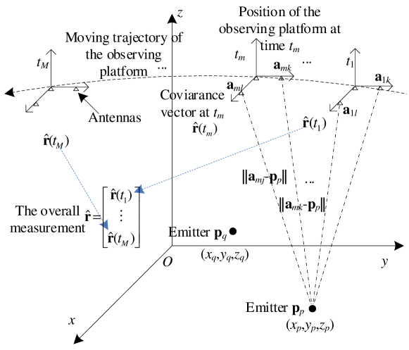
Figure 1: The localization model.

1.3 Notations

In this paper, diag( ) denotes making a diagonal matrix with the elements of the vector. The notations $||\cdot||{}_{1}$, $||\cdot||$ denote the ${\ell_{1}}$, and ${\ell_{2}}$-norm of the matrix, respectively. The superscripts ^∗, ^T, ^H denote the conjugation, transposition, conjugate transposition of the matrix, respectively. The notation vec( ) denotes the vectorization operator of a matrix.

2 Covariance sparse representation based multi-target localization

We look into a localization problem for multiple targets from a moving platform. As an example shown in Fig. 1, an observing platform, such as a satellite or an unmanned aerial vehicle, moves along its trajectory. A planar antenna array is installed on the moving platform to intercept the signals transmitted from the emitters. The real-time positions of the platform can be obtained by its own positioning devices, such as a GPS receiver. The task of the localization problem is to estimate the positions of the targets.

In the traditional ways, the positions of the targets are obtained using a BOL or the phase difference rate. Here, we propose a new signal model to solve the localization problem.

Without loss of generality, the coordinate system of the moving platform is the same with geodetic coordinate system all the time for simplicity. The signals could not be intercepted all the time, but only are available at discontinuous slow time instants ${t_{m}}$, $m=1,...,M$, because of the noncooperative receiver. We do not require that the signals are coherent for all the slow time instants because the crystal on the receiver of the moving platform could not keep stable for a long period. Instead, we just need to calculate the covariant matrix of the signals from the antenna array only at the instant ${t_{m}}$, $m=1,...,M$, respectively.

The planar array consists of L antenna elements. Let ${{\bf{a}}_{ml}}$ denote the position of the antenna l, l=1,…,L at the instant ${t_{m}}$, $m=1,...,M$. The antenna array is either uniformly or randomly distributed, while the latter can break through the half-wavelength limitation of the array, eliminate the grating lobe, and result in improved property for the over-complete dictionary and offer more robust reconstruction. The receiver intercepts the signals emitted from the target position ${{\bf{p}}_{p}}:={[{x_{p}},{y_{p}},{z_{p}}]^{T}}$, $p=1,...,K$, where K is the number of the emitters. The task of the localization is to estimate ${{\bf{p}}_{p}}$ from the signals impinging on the array at several instants ${t_{m}}$, $m=1,...,M$. Here, the time instants ${t_{m}}$ are called the slow time.

The K narrowband signals, ${{\bf{s}}_{\rm{r}}}({t_{m,n}})\in{{}^{L}}$, impinging on the L antennas are received during a short period at time ${t_{m}}$ containing N snapshots, which can be expressed as:

$${{\bf{s}}_{\rm{r}}}({t_{m,n}})={\bf{A}}({t_{m}}){\bf{s}}({t_{m,n}})+{{\bf{n}}_{\rm{r}}}({t_{m,n}})$$ (1)

where ${\bf{s}}({t_{m,n}})\in{{}^{K\times 1}}$ is complex envelope of the incoherent signals transmitted from K emitters, ${t_{m,n}},n=1,...,N$ is the fast time instant. Assume that the interval between the slow time ${t_{m}}$ and ${t_{m+1}}$ is much greater than the period of N snapshots lasting in the fast time. The entries of ${{\bf{s}}_{\rm{r}}}({t_{m,n}})$ are the complex envelopes of the summation of all the signals received on the antennas at the time instant ${t_{m,n}}$. The noise vector ${{\bf{n}}_{\rm{r}}}({t_{m,n}})$ is the additive circular complex Gaussian white noise with zero mean and variance $\sigma_{n}^{2}$, which is uncorrelated with ${\bf{s}}({t_{m,n}})$. The notation ${\bf{A}}({t_{m}})\in{{\bf{C}}^{K\times L}}$ is the array-steering matrix at time ${t_{m}}$, and it may be varying with time ${t_{m}}$ because of the moving measurement platform. However, we assume that ${\bf{A}}({t_{m}})$ is constant within the period of N snapshots lasting in the fast time, which is defined as

$${\bf{{\rm A}}}({t_{m}})=[{{\bf{\alpha}}_{1}}({t_{m}}),{\kern 1.0pt}{\kern 1.0pt}{{\bf{\alpha}}_{2}}({t_{m}}){\kern 1.0pt}{\kern 1.0pt},{\kern 1.0pt}{\kern 1.0pt}...{\kern 1.0pt}{\kern 1.0pt}{\kern 1.0pt}{\kern 1.0pt},{{\bf{\alpha}}_{K}}({t_{m}})]$$ (2)

where

$${{\bf{\alpha}}_{p}}({t_{m}})={[1{\kern 1.0pt}{\kern 1.0pt}{\kern 1.0pt}{\kern 1.0pt}{e^{-j2\pi f(||{{\bf{a}}_{m2}}-{{\bf{p}}_{p}}||-||{{\bf{a}}_{m1}}-{{\bf{p}}_{p}}||)/c}}...{e^{-j2\pi f(||{{\bf{a}}_{mL}}-{{\bf{p}}_{p}}||-||{{\bf{a}}_{m1}}-{{\bf{p}}_{p}}||)/c}}]^{T}},$$

is the array-steering vector of frequency $f$ and is with respect to the emitter’s position ${{\bf{p}}_{p}}$. As illustrated in Fig. 1, ${{\bf{a}}_{ml}}$ is the position of the lth antenna at the time instant ${t_{m}}$, and $||{{\bf{a}}_{ml}}-{{\bf{p}}_{p}}||$ is the distance between the lth antenna and the pth emitter. Different from the traditional approaches in [5] and [6], the array-steering matrix here is more directly and conveniently defined with respect to the emitter’s position ${{\bf{p}}_{p}}$, without any approximation. This definition is easier to calculate the derivations, which will be given in the Appendix.

Thus, the array covariance matrix of the received signals at time ${t_{m}}$ is given by

$${\bf{R}}({t_{m}})=E[{{\bf{s}}_{\rm{r}}}({t_{m}}){\bf{s}}_{\rm{r}}^{H}({t_{m}})]={\bf{A}}({t_{m}}){\bf{\mathcal{S}}}{{\bf{A}}^{H}}({t_{m}})+\sigma_{n}^{2}{{\bf{I}}_{L}}$$ (3)

where E[ ] denotes the expectation operator, and ${{\bf{I}}_{L}}$is the identity matrix of order $L\times L$. The source covariance matrix ${\bf{\mathcal{S}}}$ is diagonal defined as ${\bf{\mathcal{S}}}=E[{\bf{s}}({t_{m}}){{\bf{s}}^{H}}({t_{m}})]=$$diag({[\sigma_{1}^{2},...,\sigma_{K}^{2}]^{T}})$, where $\sigma_{1}^{2},...,\sigma_{K}^{2}$ denote the power of the signals.

Let ${\bf{r}}({t_{m}})$ be the covariance vector defined as the vectorized covariance matrix ${\bf{r}}({t_{m}})=vec({\bf{R}}({t_{m}}))$. From (3), we get [15]

$${\bf{r}}({t_{m}})={\bf{\Psi}}({t_{m}}){\boldsymbol{\rho}}+\sigma_{n}^{2}vec({{\bf{I}}_{L}})$$ (4)

where

$${\bf{\Psi}}({t_{m}}):=[{\bf{\alpha}}_{{{\bf{p}}_{1}}}^{*}({t_{m}})\otimes{{\bf{\alpha}}_{{{\bf{p}}_{1}}}}({t_{m}}),...,{\bf{\alpha}}_{{{\bf{p}}_{K}}}^{*}({t_{m}})\otimes{{\bf{\alpha}}_{{{\bf{p}}_{K}}}}({t_{m}})]$$ (5)

${\boldsymbol{\rho}}:={[\sigma_{1}^{2},...,\sigma_{K}^{2}]^{T}}$, and $\otimes$ denotes the Kronecker product.

Equation (4) is just a theoretical model of the array covariance vector. However, in reality, ${\bf{r}}({t_{m}})$ must be estimated by

$${\bf{\hat{r}}}({t_{m}})=vec[{\bf{\hat{R}}}({t_{m}})]=vec\left[{\frac{1}{N}\sum\limits_{n={\rm{1}}}^{N}{{{\bf{s}}_{\rm{r}}}({t_{m,n}}){\bf{s}}_{\rm{r}}^{H}({t_{m,n}})}}\right]$$ (6)

Therefore, ${\bf{\hat{r}}}({t_{m}})$ is not an ideal covariance vector any more, while it contains some noise terms, such as the signal-to-signal and the signal-to-noise cross-terms. Thus, the model can be rewritten as

$${\bf{\hat{r}}}({t_{m}})={\bf{\Psi}}({t_{m}}){\boldsymbol{\rho}}+\sigma_{n}^{2}vec({{\bf{I}}_{L}})+{\bf{n}}({t_{m}})$$ (7)

where ${\bf{n}}({t_{m}})$ is the estimation error following the asymptotically Gaussian distribution [16]

$${\bf{n}}({t_{m}})\sim(0,\frac{1}{N}{{\bf{R}}^{T}}({t_{m}})\otimes{\bf{R}}({t_{m}}))$$ (8)

Obviously, ${\boldsymbol{\rho}}$ cannot be solved from a measurement of a single observation position. Therefore, we use all the measurements of different time instants from different observing positions. Thus, we stack all the measurements at all the available instants to form a complete model

$${\bf{\hat{r}}}={\bf{\Psi\rho}}+{\bf{n}}$$ (9)

where

$${\bf{n}}={[\begin{array}[]{*{20}{c}}{{{\bf{n}}^{T}}({t_{1}})}&\cdots&{{{\bf{n}}^{T}}({t_{M}})}\end{array}]^{T}},$$

$${\bf{\hat{r}}}=\left[{\begin{array}[]{*{20}{c}}{{\bf{\hat{r}}}({t_{1}})}\\ \cdots\\ {{\bf{\hat{r}}}({t_{M}})}\end{array}}\right]-\sigma_{n}^{2}\left[{\begin{array}[]{*{20}{c}}{vec({{\bf{I}}_{L}})}\\ \cdots\\ {vec({{\bf{I}}_{L}})}\end{array}}\right],$$

$${\bf{\Psi}}=\left[{\begin{array}[]{*{20}{c}}{{\bf{\Psi}}({t_{1}})}\\ \vdots\\ {{\bf{\Psi}}({t_{M}})}\end{array}}\right]$$ (10)

The construction of the measurement ${\bf{\hat{r}}}$ is also illustrated as in Fig. 1. In the measuring model of (9) for multiple instants, the estimation error of the covariance vector also follows the asymptotically Gaussian distribution, that is,

$${\bf{n}}\sim(0,{\bf{C}})$$ (11)

with the covariance matrix

$${\bf{C}}=\frac{1}{N}\left[{\begin{array}[]{*{20}{c}}{{{\bf{R}}^{T}}({t_{1}})\otimes{\bf{R}}({t_{1}})}&{}\hfil&{}\hfil\\ {}\hfil&\ddots&{}\hfil\\ {}\hfil&{}\hfil&{{{\bf{R}}^{T}}({t_{M}})\otimes{\bf{R}}({t_{M}})}\end{array}}\right]$$ (12)

3 Off-grid Compressive Sensing Based Localization

3.1 Off-grid Localization Model

In the classical algorithms, the positions of candidate emitters are assumed to lie on some fixed discrete grids, so that the conventional compressive sensing can take into effect. The continuous space has to be discretized to a finite set of points, and signals are represented sparsely in a fixed known dictionary. However, in practical localization problems, the emitters do not necessarily lie on these grids exactly. For the purpose of obtaining a higher estimation precision, the grids are needed to be refined. However, the refined grids will increase the coherence of the measurement matrix, which will in turn limit the performance of the algortihm [8].

Thus, the dictionary should be represented by the positions in a continuous domain. The dictionary can’t be preset any more. The off-grid localization becomes a joint dictionary learning and emitter position estimation problem.

Without dividing the target area into uniform grids, the signal model of (9) should be modified to:

$${\bf{\hat{r}}}={\bf{\Psi}}(\mathcal{S}){\boldsymbol{\rho}}+{\bf{n}}$$ (13)

where ${\bf{\Psi}}(\mathcal{S}):=[{\boldsymbol{\psi}}({{\bf{p}}_{1}}),...,{\boldsymbol{\psi}}({{\bf{p}}_{K}})]\in{{}^{{L^{2}}M\times P}}$, ${\bf{\hat{r}}}$, ${\boldsymbol{\rho}}$ and ${\bf{n}}$ are the same as defined in (9). Define a set of the emitters’ positions, $\mathcal{S}:=\{{{\bf{p}}_{p}}{\rm{\}}}_{p=1}^{P}$, and ${\boldsymbol{\psi}}({{\bf{p}}_{p}})$, the column of ${\bf{\Psi}}(\mathcal{S})$, is the function of a position ${{\bf{p}}_{p}}$ in the continuous domain.

Thus, the off-grid localization problem is not only estimating the signal power, but also adjusting the position parameters of the atoms, ${\boldsymbol{\psi}}({{\bf{p}}_{p}})$, to attain their true values. Off-grid CS offers improved resolution and robust performance because of the sparsity constraint. The goal is to search for the unknown dictionary composed of as few atoms as possible. Thus, the off-grid localization problem can expressed as the following $l_{0}^{\lambda}$-minimization:

$$\mathop{\min}\limits_{\mathcal{S},{\boldsymbol{\rho}}}\quad\lambda||\boldsymbol{\rho}||_{0}+||{\bf{\hat{r}}}-{\bf{\Psi}}(\mathcal{S}){\boldsymbol{\rho}}|{|^{2}}$$ (14)

3.2 Sparse recovery model and its alternative model

Because $\ell_{0}$-norm is a discrete integer function, $\ell_{0}^{\lambda}$-minimization is a NP-HARD problem [25], so we consider the following alternative function $g_{\delta}(\cdot)$ to replace $\ell_{0}$-norm:

$$\mathop{\min}\limits_{\mathcal{S},{\boldsymbol{\rho}}}\quad\mathcal{G}(\mathcal{S},{\boldsymbol{\rho}}):=\lambda g({\boldsymbol{\rho}})+||{\bf{\hat{r}}}-{\bf{\Psi}}(\mathcal{S}){\boldsymbol{\rho}}|{|^{2}},$$ (15)

The objective function

$$g_{\delta}({\boldsymbol{\rho}})=\sum\limits_{p=1}^{P}{g_{c}(\rho_{p})}=\sum\limits_{p=1}^{P}{atan|\rho_{p}/\delta|}$$ (16)

can be separated to a summation of several objective function, where ${\rho_{p}}$ represents the pth entry of ${\boldsymbol{\rho}}$. The scalar function ${atan|\rho/\delta|}$ is sign invariant and concave-and-monotonically increasing on the non-negative orthant ${\mathcal{O}_{1}}$. $\lambda>0$ is a regularization parameter to provide a trade-off between fidelity to the measurements and sparsity in the optimal solution.

However, the minimization problem (14) and (15) are difficult to solve since there are two optimization variables $\mathcal{S}$ and $\boldsymbol{\rho}$, so we adopt alternating optimization strategy to solve this problem. Among the processing of alternating optimization, the update of $\boldsymbol{\rho}$ is the most important aspect, since a accurate solution of the present sparse model can provide a more reasonable modification of the grid point set $\mathcal{S}$.

In sparse recovery theory, the main algorithms designed for solve model (14) can be divided into two categories, greedy algorithms, such as OMP and convex relaxation methods, such as $l_{1}$-minimization. Although greedy algorithms are designed to solve model (14) directly, due to the fact that model (14) is a NP-HARD problem [25], these algorithms only performance well with a low level. Furthermore, convex relaxation methods need the measurement matrix ${\bf{\Psi}}(\mathcal{S}$ to meet the Restricted Isometry Property (RIP). A matrix $A$ is said to satisfy RIP of order $2k$ if and only if there exists a constant $\delta_{2k}\in(0,1)$ such that

$$(1-\delta_{2k})\|x\|_{2}^{2}\leq\|Ax\|_{2}^{2}\leq(1+\delta_{2k})\|x\|_{2}^{2}$$ (17)

for any $2k$ sparse vector $x$. In [27], it has been proved that $\delta_{2k}\leq\sqrt{2}/2$ is the theoretical optimal conditions to recover the real sparse solution by $l_{1}$-minimization. However, to verify RIP for a given matrix ${\bf{\Psi}}(\mathcal{S}$ also is a NP-HARD problem [28]. Therefore, at each iteration, it is important to ensure $g_{\delta}({\boldsymbol{\rho}})$ can recover the real sparse solution without any request of ${\bf{\Psi}}(\mathcal{S})$. Furthermore, the following theorem offer us a guarantee for the alternative function $g_{\delta}({\boldsymbol{\rho}})$ for sparse recovery.

Theorem 1.

For a given $\mathcal{S}$, there exist a constant $\delta(\mathcal{S},\lambda)$ such that both of the following minimization problems

$$\mathop{\min}\limits_{{\boldsymbol{\rho}}}\quad\lambda||\boldsymbol{\rho}||_{0}+||{\bf{\hat{r}}}-{\bf{\Psi}}(\mathcal{S}){\boldsymbol{\rho}}|{|^{2}}$$ (18)

and

$$\mathop{\min}\limits_{{\boldsymbol{\rho}}}\quad\mathcal{G}(\mathcal{S},{\boldsymbol{\rho}}):=\lambda g({\boldsymbol{\rho}})+||{\bf{\hat{r}}}-{\bf{\Psi}}(\mathcal{S}){\boldsymbol{\rho}}|{|^{2}}$$ (19)

share the same sparse solutions whenever $0<\delta<\delta(\mathcal{S},\lambda)$.

Proof.

See Appendix for more details. ∎

3.3 Iterative Reweighted MM Algorithm

However, the complicated objective functions render the direct problem solving intractable. A simple iterative algorithm is proposed here by exploiting the MM technique to minimize the objective function of (15) by using a surrogate convex function. In each iteration, the algorithm alternates between estimating ${\boldsymbol{\rho}}$ and refining the location set ${\mathcal{S}}$.

The goal of the proposed algorithm is to find a convex smooth function ${f_{\rm{c}}}(\rho)$ to replace ${g_{\rm{c}}}(\rho)$ in an iterative way, and ${f_{\rm{c}}}(\rho)$ should be chosen for easy minimizing. According to the MM technique, the surrogate function should be selected satisfying two conditions. One is it should majorize the original function, the other is its global minimization must guarantee the original objective function reducing.

Many methods are proposed for constructing surrogate objective functions. One of them is construction by second order Taylor expansion [21]. There exists a value such that , making the following inequality hold [20]:

$$\begin{array}[]{l}{g_{\rm{c}}}(\rho)\leq\\ {g_{\rm{c}}}({\rho^{(i)}})+{\left.{\frac{{\partial{g_{\rm{c}}}(\rho)}}{{\partial\rho}}}\right|_{\rho={\rho^{(i)}}}}(\rho-{\rho^{(i)}})+\frac{1}{2}{\beta^{(i)}}{(\rho-{\rho^{(i)}})^{2}}\end{array}$$ (20)

where ${\partial{g_{\rm{c}}}(\rho)\over{\partial\rho}}={\delta\rho\over{|\rho|(\delta^{2}+\rho^{2})}}$ is the gradient of ${g_{\rm{c}}}({\rho})$. Hence, we can define a surrogate function for the ith iteration:

$$\begin{array}[]{l}{f_{\rm{c}}}(\rho|{\rho^{(i)}})=\\ {g_{\rm{c}}}({\rho^{(i)}})+{\left.{\frac{{\partial{g_{\rm{c}}}(\rho)}}{{\partial\rho}}}\right|_{\rho={\rho^{(i)}}}}(\rho-{\rho^{(i)}})+\frac{1}{2}{\beta^{(i)}}{(\rho-{\rho^{(i)}})^{2}}\end{array}$$ (21)

From (14), we notice that $g({\boldsymbol{\rho}})$ is a summation of ${g_{\rm{c}}}(\rho)$, so the surrogate function of $g({\boldsymbol{\rho}})$ for the ith iteration, denoted by $f({\boldsymbol{\rho}}|{{\boldsymbol{\rho}}^{(i)}})$, can be derived from the above scalar component ${f_{\rm{c}}}(\rho|{\rho^{(i)}})$:

$$\begin{array}[]{l}f({\boldsymbol{\rho}}|{{\boldsymbol{\rho}}^{(i)}})=\sum\limits_{p=1}^{P}{{f_{\rm{c}}}({\rho_{p}}|\rho_{p}^{(i)})}\\ =g({{\boldsymbol{\rho}}^{(i)}})+{({\boldsymbol{\rho}}-{{\boldsymbol{\rho}}^{(i)}})^{T}}{\left.{\frac{{\partial g({\boldsymbol{\rho}})}}{{\partial{\boldsymbol{\rho}}}}}\right|_{{\bf{\rho}}={{\boldsymbol{\rho}}^{(i)}}}}+{({\boldsymbol{\rho}}-{{\bf{\rho}}^{(i)}})^{T}}{{\bf{B}}^{(i)}}({\boldsymbol{\rho}}-{{\boldsymbol{\rho}}^{(i)}})\end{array}$$ (22)

where ${\left.{{\textstyle{{\partial g({\boldsymbol{\rho}})}\over{\partial{\bf{\rho}}}}}}\right|_{{\boldsymbol{\rho}}={{\boldsymbol{\rho}}^{(i)}}}}={[{\left.{{\textstyle{{\partial{g_{\rm{c}}}(\rho)}\over{\partial\rho}}}}\right|_{\rho=\rho_{1}^{(i)}}},...,{\left.{{\textstyle{{\partial{g_{\rm{c}}}(\rho)}\over{\partial\rho}}}}\right|_{\rho=\rho_{P}^{(i)}}}]^{T}}$ is the gradient of $g({\boldsymbol{\rho}})$ at ${\boldsymbol{\rho}}={{\boldsymbol{\rho}}^{(i)}}$, and

$${{\bf{B}}^{(i)}}=diag({\textstyle{{\rm{1}}\over{\rm{2}}}}\beta_{1}^{(i)},...,{\textstyle{{\rm{1}}\over{\rm{2}}}}\beta_{P}^{(i)})$$ (23)

at the ith iteration. Ignoring terms irrelevant to the variable ${\boldsymbol{\rho}}$, the surrogate function becomes to the following equivalent form:

$$f({\boldsymbol{\rho}}|{{\boldsymbol{\rho}}^{(i)}})={{\boldsymbol{\rho}}^{T}}\left({{{\left.{\frac{{\partial g({\boldsymbol{\rho}})}}{{\partial{\boldsymbol{\rho}}}}}\right|}_{{\bf{\rho}}={{\boldsymbol{\rho}}^{(i)}}}}-2{{\bf{B}}^{(i)}}g({{\boldsymbol{\rho}}^{(i)}})}\right)+{{\boldsymbol{\rho}}^{T}}{{\bf{B}}^{(i)}}{\boldsymbol{\rho}}$$ (24)

Inspired by the idea presented in [20], (24) can be further simplified to a more compact version by selecting ${{\bf{B}}^{(i)}}$ to make ${\left.{{\textstyle{{\partial g({\boldsymbol{\rho}})}\over{\partial{\boldsymbol{\rho}}}}}}\right|_{{\boldsymbol{\rho}}={{\boldsymbol{\rho}}^{(i)}}}}-2{{\bf{B}}^{(i)}}g({{\bf{\rho}}^{(i)}})={\rm{0}}$. Finally, the surrogate function can be expressed as:

$$f({\boldsymbol{\rho}}|{{\boldsymbol{\rho}}^{(i)}})={{\boldsymbol{\rho}}^{T}}{{\bf{B}}^{(i)}}{\boldsymbol{\rho}}$$ (25)

where the diagonal elements satisfy

$$\beta_{p}^{(i)}={{{{\left.{{\textstyle{{\partial{g_{\rm{c}}}(\rho)}\over{\partial\rho}}}}\right|}_{\rho=\rho_{p}^{(i)}}}}\mathord{\left/{\vphantom{{{{\left.{{\textstyle{{\partial{g_{\rm{c}}}(\rho)}\over{\partial\rho}}}}\right|}_{\rho=\rho_{p}^{(i)}}}}{{g_{\rm{c}}}(\rho_{p}^{(i)})}}}\right.\kern-1.2pt}{\rho_{p}^{(i)}}}={\delta\over{|\rho|(\delta^{2}+\rho^{2})}}$$ (26)

Resolving the unconstrained optimization of (19) by an iterative optimization method using the surrogate function of (25), the sub-problem of (19) at the (i)th iteration can be expressed as:

$$\mathop{\min}\limits_{\mathcal{S},{\boldsymbol{\rho}}}\mathcal{L}(\mathcal{S},{\boldsymbol{\rho}}):=\lambda{{\boldsymbol{\rho}}^{T}}{{\bf{B}}^{(i)}}{\boldsymbol{\rho}}+||{\bf{\hat{r}}}-{\bf{\Psi}}(\mathcal{S}){\boldsymbol{\rho}}|{|^{2}}$$ (27)

3.4 Alternatively Optimizing

From (27), it is still intractable to optimize the objective function respect to and ${\boldsymbol{\rho}}$ simultaneously. Hence, and ${\boldsymbol{\rho}}$ should be optimized alternatively at the (i+1)th iteration. First, suppose is estimated at the ith iteration, so conditioned on , taking the complex gradient [22] of it with respect to ${\boldsymbol{\rho}}$, and setting the gradient to zero and solving the equation, one can obtain the minimum point at the (i+1)th iteration as follows:

$$\begin{array}[]{c}{{\boldsymbol{\rho}}^{(i+1)}}={\left({{\mathop{\rm Re}\nolimits}\left({{{\bf{\Psi}}^{H}}({\mathcal{S}^{(i)}}){\bf{\Psi}}(\mathcal{S}{{}^{(i)}})}\right)+{\lambda}{{\bf{B}}^{(i)}}}\right)^{-1}}\\ \cdot{\mathop{\rm Re}\nolimits}\left({{{\bf{\Psi}}^{H}}(\mathcal{S}{{}^{(i)}}){\bf{\hat{r}}}}\right)\end{array}$$ (28)

We observe that the optimal ${{\boldsymbol{\rho}}^{(i+1)}}$ can be expressed by an explicit solution such that the calculation complexity of this step can be dramatically reduced compared with ${\ell_{1}}$ minimization method such as described in [19].

Theorem 2.

Given a solution ${{\boldsymbol{\rho}}^{(i)}}$ of the ith iteration, ${{\bf{B}}^{(i)}}$ is calculated by using (26). If a new solution of the (i+1)th iteration, ${{\boldsymbol{\rho}}^{(i+1)}}$, is obtained by (28), then the objective function of the original problem (15) satisfies:

$$\Gamma(\mathcal{S}{{}^{(i)}},{{\boldsymbol{\rho}}^{(i+1)}})\leq\Gamma(\mathcal{S}{{}^{(i)}},{{\boldsymbol{\rho}}^{(i)}})$$ (29)

where the equation holds only if ${{\boldsymbol{\rho}}^{(i)}}$ is a fixed point of (15).

Proof.

Because ${g_{\rm{c}}}(\rho)$ is sign invariant (i.e., ${g_{\rm{c}}}(\rho)={g_{\rm{c}}}(|\rho|)$), and concave-and-monotonically increasing on the non-negative orthant ${\mathcal{O}_{1}}$, $g({\boldsymbol{\rho}})$ is sign invariant and concave on its ${\mathcal{O}_{1}}$. From (22), we can get:

$$g({{\boldsymbol{\rho}}^{(i)}})=f({{\boldsymbol{\rho}}^{(i)}}|{{\boldsymbol{\rho}}^{(i)}}),{\left.{\frac{{\partial g({\boldsymbol{\rho}})}}{{\partial{\boldsymbol{\rho}}}}}\right|_{{\bf{\rho}}={{\boldsymbol{\rho}}^{(i)}}}}={\left.{\frac{{\partial f({\boldsymbol{\rho}}|{{\bf{\rho}}^{(i)}})}}{{\partial{\boldsymbol{\rho}}}}}\right|_{{\boldsymbol{\rho}}={{\bf{\rho}}^{(i)}}}}$$ (30)

And also because of the selection of ${{\bf{B}}^{(i)}}$ as (26), $f({\boldsymbol{\rho}}|{{\boldsymbol{\rho}}^{(i)}})$ is convex, majorizes $g({\boldsymbol{\rho}})$, and shares the same tangent with $g({\boldsymbol{\rho}})$ at the point ${{\bf{\rho}}^{(i)}}$ on ₁ (as illustrated in Fig. 2). These are also true for the other ${2^{P}}-1$ orthants. We have:

$$f({{\boldsymbol{\rho}}^{(i+1)}}|{{\boldsymbol{\rho}}^{(i)}})-g({{\boldsymbol{\rho}}^{(i+1)}})\geq f({{\boldsymbol{\rho}}^{(i)}}|{{\boldsymbol{\rho}}^{(i)}})-g({{\boldsymbol{\rho}}^{(i)}})=0$$ (31)

where the equation holds only if ${{\boldsymbol{\rho}}^{(i)}}$ is a fixed point, i.e.

$|{{\boldsymbol{\rho}}^{(i+1)}}|=|{{\boldsymbol{\rho}}^{(i)}}|$. Thus, the following relationship holds:

$$g({{\boldsymbol{\rho}}^{(i+1)}})-g({{\boldsymbol{\rho}}^{(i)}})\leq f({{\boldsymbol{\rho}}^{(i+1)}}|{{\boldsymbol{\rho}}^{(i)}})-f({{\boldsymbol{\rho}}^{(i)}}|{{\boldsymbol{\rho}}^{(i)}})$$ (32)

Because the second term of (15) is the same with that of (27), we get the conclusion of (29). ∎

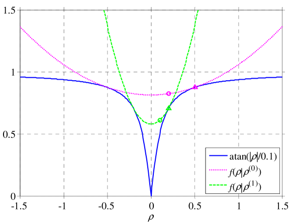
Figure 2: Illustration of the surrogate function at different iterations.

Theorem 2 guarantees that the surrogate function of (27) can equivalently reduce the objective function of (15) in an iterative way.

After updating ${\boldsymbol{\rho}}$ at the (i+1)th iteration, the second step is to adjust the parameter set, $\mathcal{S}$ , to obtain refined target positions, by substituting (28) into (27):

$$\begin{array}[]{c}\mathop{\min}\limits_{\mathcal{S}}\mathcal{L}(\mathcal{S})=-2{\mathop{\rm Re}\nolimits}\left({{{{\bf{\hat{r}}}}^{H}}{\bf{\Psi}}(\mathcal{S}{{}^{(i)}})}\right)\cdot{\left({{\mathop{\rm Re}\nolimits}\left({{{\bf{\Psi}}^{H}}({{}^{(i)}}){\bf{\Psi}}({{}^{(i)}})}\right)+{\lambda}{{\bf{B}}^{(i)}}}\right)^{-1}}\cdot{\mathop{\rm Re}\nolimits}\left({{{\bf{\Psi}}^{H}}(\mathcal{S}{{}^{(i)}}){\bf{\hat{r}}}}\right)\end{array}$$ (33)

From (33), one can observe that it’s still hard to get an solution of $\mathcal{S}$ which minimizes the objective function $\mathcal{L}(\mathcal{S})$. Fortunately, the minimization procedure can be replaced by simply finding an appropriate only to reduce the objective function instead [10]. Thus, in this step we just need to find a set ${\mathcal{S}^{(i+{\rm{1}})}}$ satisfying:

$$\mathcal{L}(\mathcal{S}{{}^{(i+{\rm{1}})}})\leq\mathcal{L}(\mathcal{S}{{}^{(i)}})$$ (34)

Since $\mathcal{L}(\mathcal{S})$ is differentiable for the problem of (33), a gradient descent method can be used to find such an estimation of ⁽ⁱ⁺¹⁾. For every element in ${\mathcal{S}^{(i)}}$, i.e., ${{\bf{p}}_{p}}$ if a gradient defined as ${\textstyle{{\partial\mathcal{L}(\mathcal{S})}\over{\partial{{\bf{p}}_{p}}}}}:={[{\textstyle{{\partial\mathcal{L}(\mathcal{S})}\over{\partial{x_{p}}}}},{\textstyle{{\partial\mathcal{L}(\mathcal{S})}\over{\partial{y_{p}}}}},{\textstyle{{\partial\mathcal{L}(\mathcal{S})}\over{\partial{z_{p}}}}}]^{T}}$ can be calculated (see Appendix for more details), we can always find a scale C which makes

$${\bf{p}}_{p}^{(i+1)}={\bf{p}}_{p}^{(i)}-C{\left.{\frac{{\partial\mathcal{L}(\mathcal{S})}}{{\partial{{\bf{p}}_{p}}}}}\right|_{{{\bf{p}}_{p}}={\bf{p}}_{p}^{(i)}}}$$ (35)

satisfying (34). When all the elements in ${\mathcal{S}^{(i)}}$ are updated, a new ${\mathcal{S}^{(i+{\rm{1}})}}$ is found at the (i+1)th iteration of the off-grid localization algorithm. The complete algorithm of the off-grid localization is described as follows.

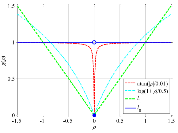
Figure 3: Comparison of objective functions with a scalar variable.

Algorithm 1 Off-grid localization algorithm based on iteratively reweighted method

0:  Set $i=0$, an initial value $\mathcal{S}^{(0)}$,$\hat{\bf{\Psi}^{(0)}}$ and $\bf{B}^{(0)}=\bf{I}$

0:  $\mathcal{S}$, $\boldsymbol{\rho}$

  Step 1. Estimate the power $\boldsymbol{\rho}^{(i+1)}$, of signals by (24).

  Step 2. Update every element by (31) to get a new $\mathcal{S}^{(i+1)}$.

  Step 3. Calculate the weight $\bf{B}^{(i+1)}$ by (22)

  Step 4. Pruning the set $\mathcal{S}^{(i+1)}$

  Step 5. Let $i=i+1$, and repeat Step 1 through 4 when $\|\boldsymbol{\rho}^{(i+1)}-\boldsymbol{\rho}^{(i)}\|\leq\varepsilon$

3.5 Discussions

3.5.1 Initialize

The proposed MM based algorithm may still converge to a local minimum, since the original objective function is non-convex. However, the existence of the sparse encouraging objective function with the regularization parameter $\lambda$ and initial set ${\mathcal{S}^{({\rm{0}})}}$ properly selected will somehow partially improve the situation.

In the initialization step of the algorithm, the localization area can be uniformly divided into some coarse grids only fine enough to prevent the algorithm from falling into some unpredictable local minimizations. The coarse grids will dramatically reduce the computational complexity.

3.5.2 Pruning

Since the localization is a typical sparse recovery problem, the computational complexity can be reduced by pruning operations. At each iteration, those signals with small powers can be pruned from the original set ${\mathcal{S}^{(i+{\rm{1}})}}$ and the vector ${{\boldsymbol{\rho}}^{(i+1)}}$. A hard threshold $\tau$ can be used to decide which signal needs to be removed, i.e., $\rho_{p}^{(i+1)}<\tau$. Hence, the dimension of the signal power ${{\boldsymbol{\rho}}^{(i+1)}}$ and the position set ⁽ⁱ⁺¹⁾ shrinks at some iterations.

By the definition of ${\ell_{0}}$-norm, the sparse original model has the ability to make energy gather on the certain location, but other continuous alternative methods, such as reweighted ${\ell_{1}}$-norm or log-sum penalty, need some strict condition of measurement matrices or lack the theoretical guarantee to ensure recover sparse solution. Compared with these methods, we have proved in Theorem 1 that the proposed method in this paper has the same ability as ${\ell_{0}}$-norm. Therefore, $atan|\rho/\delta|$

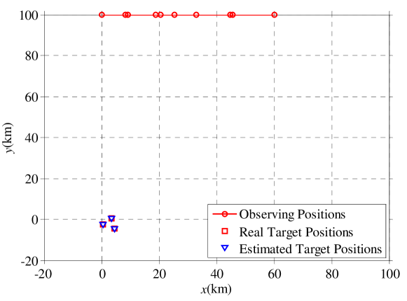
Figure 4: Localization geometry for the simulations.

can better approximate the ${\ell_{0}}$ penalty than ${\rm{log}}|\rho|$. It has the potential to be more sparsity encouraging than the reweighted ${\ell_{1}}$-norm and the log-sum penalty function [19].

Fig. 3 shows the shapes of different objective functions with respect to a scalar variable $\rho$. Notice that $atan|\rho/\delta|$ is more like ${\ell_{0}}$ penalty function than ${\rm{log}}|\rho|$. The smaller the parameter $\delta>0$ becomes, the more similar $atan|\rho/\delta|$ is to ${\ell_{0}}$.

4 Numerical Simulations

In this section, numerical experiments are performed to proof the promise of the proposed localization estimation model using sparse representation of array covariance matrix.

The localization geometry is depicted in Fig. 4. The circle markers represent the positions of the reference antenna on a moving observing platform at different time instances. The solid line represents the trajectory of the moving array. The length of the solid line denotes the overall virtual aperture. The virtual aperture is the maximum distance between the observing positions. The antenna array in the simulations is a non-uniform linear array, and the antennas are randomly distributed along x

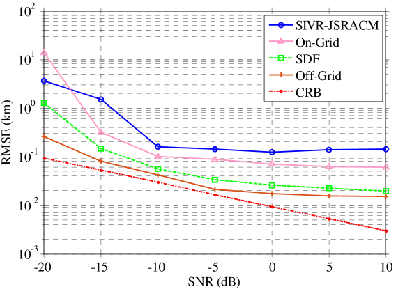
Figure 5: RMSE of different methods.

coordinates in the range of $[0,D]$, relative to the reference antenna, where D is the real array aperture. The coordinates of the closely spaced targets are [0.5140, -2.4755], [3.5106, 0.5102], [4.5115, -4.4876].

We carry out the simulation experiment to compare the performance with the existing popular algorithms in Fig. 5. The experiment conditions are as follows. The carrier frequencies of the signals are 6GHz. The real array aperture D=4m, the number of the observing points M is 10, and the number of the array elements L is 11. The number of the snapshot at each observing points is N=1000. The performance of the localization algorithm is measured by means of the root mean square error (RMSE), which is defined as the average of Q independent Monte Carlo trials, that is,

$$RMSE=\sqrt{\frac{1}{{P\cdot Q}}\sum\limits_{q=1}^{Q}{\sum\limits_{p=1}^{P}{||{\bf{\hat{p}}}_{p}^{(q)}-{\bf{p}}_{p}^{(q)}|{|^{2}}}}}$$ (36)

The line with circle markers represents the JSRACM algorithm of [6], and the line with square markers is the subspace data fusion (SDF) algorithm of [5]. The lines with markers ‘triangle’ and ‘plus’ represent the proposed on-grid and off-grid algorithm respectively. The CRB is a line with dot markers, and

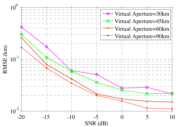
Figure 6: RMSE for different virtual apertures.

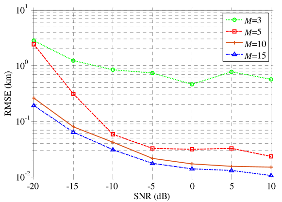
Figure 7: RMSE for different numbers of observing points.

the calculation of CRB is given in the Appendix B. The experimental condition is the same for each algorithm. The grid resolution of the JSRACM and SDF algorithm is set to 25m. High grid resolution results in very high computational complexity. As demonstrated in Fig. 5, the localization performance is greatly improved by using the proposed off-grid algorithm.

The RMSEs of the localization for different virtual apertures are shown in Fig.6. The experiment’s condition is the same as the first one, except that the virtual aperture varies from 30km to 90km. We observe that the localization precision is approximately proportional to the virtual aperture. However, when the virtual aperture is too small, the off-grid algorithm is easy to fall into a local minimum value to fail the localization.

The number of the observing points has a considerably

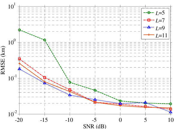
Figure 8: RMSE for different numbers of antennas.

Figure 9: RMSE for different numbers of targets.

impact on the localization precision as in Fig.7. A comparatively small M is needed in the proposed algorithm. It is only needed to be large enough to meet the demand of the observing condition. That is a good property for most localization problems because numerous observing sites are often unavailable. For instance, in the passive surveillance, the intercepted signals have limited measurement samples due to the noncooperative receiving. This property significantly outweighs the phase difference rate algorithm [3], because the latter needs a large amount of consecutive observing points to track the rate. As in Fig. 8, the proposed algorithm in this paper only needs three observing points to get an acceptable performance.

The number of the antennas also has a significant influence on the localization precision. As in Fig.8, the experiment’s condition is the same as the first one, except that the number of the antennas varies from five to eleven. More antennas result in higher localization performance. However, the experiment is also inspiring in the implementation, as the proposed algorithm does not need a great number of array elements.

The proposed algorithm can also deal with the situation that the number of targets is greater than that of the antennas. As shown in Fig.9, the number of antennas is five. The SDF algorithm [5] can only estimate the positions of no more than four targets. We notice that with the number of targets increasing, the precision will relatively decrease. However, the proposed off-grid algorithm still reaches a fairly high performance even when the number of targets is greater than that of antennas.

5 Conclusions

We propose a novel one-step localization system model using the sparse representation of the array covariance matrix for both on-grid and off-grid scenarios. The simulation verifies the idea that the atan-sum is more sparsity encouraging. The experiments also show that the localization performance is more dependent on the virtual aperture, and less dependent on the number of the array elements, and the number of the observing sites. The ability of the multiple-target localization is also verified.

Appendix A Proof of Theorem 1

In order to show our proof clearly, we use $\bf{\Psi}={\bf{\Psi}}(\mathcal{S})$ for a given $\mathcal{S}$. By reference to the mathematical skill in [29], we will give a rigorous proof of the equivalence between the alternative method and the original sparse problem.

In sparse recovery problem, the core problem is to solve the following $\ell_{0}$-minimization problem,

$$\min\limits_{{\bf{x}}\in\mathbb{R}^{n}}\|{\bf{x}}\|_{0}\ \ s.t.\ {\bf{\Psi}}{\bf{x}}={\bf{b}}$$ (37)

Because $\ell_{0}$-minimization is a NP-HARD problem, so we consider the following alternative function $g_{\delta}(\cdot)$ to replace $\ell_{0}$-norm, and we can derive the corresponding $\ell_{g_{\delta}}$-minimization,

$$\min\limits_{{\bf{x}}\in\mathbb{R}^{n}}\|{\bf{x}}\|_{g_{\delta}}s.t.\ {\bf{\Psi}}{\bf{x}}={\bf{b}}$$ (38)

where $\|{\bf{x}}\|_{g_{\delta}}=\sum\limits_{i=1}^{n}g_{\delta}(x_{i})$.

In practical application, the measurement vector ${\bf{b}}$ usually contain noise, so model 37 and model 38 can be changed into the following regularization models

$$\min\|{\bf{\Psi}}{\bf{x}}-{\bf{b}}\|_{2}^{2}+\lambda\|{\bf{x}}\|_{0}$$ (39)

and

$$\min\|{\bf{\Psi}}{\bf{x}}-{\bf{b}}\|_{2}^{2}+\lambda\|{\bf{x}}\|_{g_{\delta}}$$ (40)

Therefore, the main contribution of this paper is to prove the equivalence relationship between model(39) and model(40).

Theorem 3.

[26] There exists a constant $\lambda_{0}>0$, such that the minimization problem 37 and 39 have the same solution for all $0<\lambda<\lambda_{0}$.

Next, we will prove the equivalence between $l_{g_{\delta}}$-minimization and $l_{0}$-minimization.

Lemma 1.

If ${\bf{x}}^{*}$ is solution of $l_{g_{\delta}}$-minimization, then the sub-matrix ${\bf{\Psi}}_{S}$ is column full rank, where $S=supp({\bf{x}}^{*})$

Proof.

If there exists a vector ${\bf{h}}\in Ker({\bf{\Psi}})$ such that $supp({\bf{h}})\subseteq S$. Without of generality, we note that ${\bf{x}}^{*}=[x^{*}_{1},x^{*}_{2},...,x^{*}_{n}]^{T}$. Let

$$a=\max\limits_{h_{i}\neq 0}\frac{|x^{*}_{i}|}{|h_{i}|}$$ (41)

therefore, it is easy to proof that

$$sgn(x^{*}_{i}+\alpha h_{i})=sgn(x^{*}_{i}-\alpha h_{i})=sgn(x^{*}_{i})$$

for $\alpha\in[0,a]$. Since $g_{\delta}({\bf{x}})$ is a concave function when ${\bf{x}}\geq 0$ or ${\bf{x}}\leq 0$, it is easy to get that

$$g_{\delta}(|x^{*}_{i}|) = g_{\delta}(\frac{1}{2}|x^{*}_{i}+\alpha h_{i}|+\frac{1}{2}|x^{*}_{i}-\alpha h_{i}|)$$

$$> \frac{1}{2}g_{\delta}(|x^{*}_{i}+\alpha h_{i}|)+\frac{1}{2}g_{\delta}(|x^{*}_{i}-\alpha h_{i}|)$$

Therefore,

$$\|{\bf{x}}^{*}\|_{g_{\delta}}>\frac{1}{2}\|{\bf{x}}^{*}+\alpha{\bf{h}}\|_{g_{\delta}}+\frac{1}{2}\|{\bf{x}}^{*}-\alpha{\bf{h}}\|_{g_{\delta}}$$

which contradicts the assumption condition. ∎

Theorem 4.

There exists a constant $\delta^{*}({\bf{\Psi}},{\bf{b}})$ based on ${\bf{\Psi}}$ and ${\bf{b}}$ such that the solution of $l_{g_{\delta}}$-minimization also solves $l_{0}$-minimization whenever $0<\delta<\delta^{*}({\bf{\Psi}},{\bf{b}})$.

Proof.

For fixed ${\bf{\Psi}}$ and ${\bf{b}}$, we can define the following sets,

$$V=\left\{{\bf{x}}|{\bf{\Psi}}{\bf{x}}={\bf{b}},{\bf{\Psi}}_{S}\text{ is column full rank, where }S=supp({\bf{x}})\right\}$$ (42)

and

$$W=\left\{{\bf{x}}\in V|\forall{\bf{y}}\in V,\|{\bf{x}}\|_{0}\leq\|{\bf{y}}\|_{0}\right\}$$ (43)

It is obvious that $W\subseteq V$ and easy to get the following inequality,

$$\|{\bf{x}}\|_{0}\leq\|{\bf{y}}\|_{0}+1$$ (44)

for any ${\bf{x}}\in W$ and ${\bf{y}}\in\overline{W}$, and there exists a constant $\delta({\bf{x}},{\bf{y}})$ such that

$$\|{\bf{x}}\|_{g_{\delta}}<\|{\bf{y}}\|_{g_{\delta}}$$ (45)

whenever $0<\delta<\delta({\bf{x}},{\bf{y}})$. Since the set $V$ is finite, for any ${\bf{x}}\in W$ and ${\bf{y}}\in\overline{W}$, we can conclude that

$$\|{\bf{x}}\|_{g_{\delta}}<\|{\bf{y}}\|_{g_{\delta}}$$ (46)

whenever $0<\delta<\delta^{*}({\bf{\Psi}},{\bf{b}})$, where

$$\delta^{*}({\bf{\Psi}},{\bf{b}})=\min\limits_{{\bf{x}}\in W,{\bf{y}}\in\overline{W}}\delta({\bf{x}},{\bf{y}}).$$ (47)

By the definition of $0$-norm and Lemma (1), it is obvious that the solutions of $l_{0}$-minimization belongs to the set $W$ and we can get conclusion of this theorem by (46). ∎

Lemma 2.

If ${\bf{x}}^{*}$ is the solution of $l_{g_{\delta}}^{\lambda}$-minimization, for any ${\bf{h}}$ with $supp({\bf{h}})\subseteq supp({\bf{x}}^{*})$, we have that

$$2<{\bf{b}}-{\bf{\Psi}}{\bf{x}}^{*},{\bf{\Psi}}{\bf{h}}>=\lambda\sum\limits_{i\in supp({\bf{x}}^{*})}\frac{\delta h_{i}sgn(x^{*}_{i})}{\delta^{2}+(x_{i}^{*})^{2}}$$ (48)

and

$$2({\bf{\Psi}}^{T}({\bf{b}}-{\bf{\Psi}}{\bf{x}}^{*}))_{i}=\frac{\lambda\delta sgn(x_{i}^{*})}{\delta^{2}+(x_{i}^{*})^{2}}$$ (49)

for any $i\in supp({\bf{x}}^{*})$.

Proof.

For any $t\in\mathbb{R}$ and ${\bf{h}}\in\mathbb{R}^{n}$ with $supp({\bf{h}})\subseteq supp({\bf{x}}^{*})$, it is obvious that

$$\|{\bf{\Psi}}{\bf{x}}^{*}-{\bf{b}}\|_{2}^{2}+\lambda\|{\bf{x}}^{*}\|_{g_{\delta}}\leq\|{\bf{\Psi}}({\bf{x}}^{*}+t{\bf{h}})-{\bf{b}}\|_{2}^{2}+\lambda\|{\bf{x}}^{*}+t{\bf{h}}\|_{g_{\delta}}$$ (50)

Since $supp({\bf{h}})\subseteq supp({\bf{x}}^{*})$, we can get that

$$\|{\bf{x}}^{*}+t{\bf{h}}\|_{g_{\delta}}-\|{\bf{x}}^{*}\|_{g_{\delta}}=\sum\limits_{i\in supp({\bf{x}}^{*})}\left(atan\frac{|x^{*}_{i}+t_{i}|}{\delta}-atan\frac{|x^{*}_{i}|}{\delta}\right)$$ (51)

Therefore, we can get that

$$t^{2}\|{\bf{\Psi}}{\bf{h}}\|_{2}^{2}+2t<{\bf{\Psi}}{\bf{x}}^{*}-{\bf{b}},{\bf{\Psi}}{\bf{h}}>+\lambda\sum\limits_{i\in supp({\bf{x}}^{*})}\left(atan\frac{|x^{*}_{i}+th_{i}|}{\delta}-atan\frac{|x^{*}_{i}|}{\delta}\right)\geq 0$$ (52)

Let $t>0$ and $t\rightarrow 0^{+}$, we can get that

$$2<{\bf{\Psi}}{\bf{x}}^{*}-{\bf{b}},{\bf{\Psi}}{\bf{h}}>+\lambda\lim\limits_{t\rightarrow 0^{+}}\sum\limits_{i\in supp({\bf{x}}^{*})}\frac{atan\frac{|x^{*}_{i}+th_{i}|}{\delta}-atan\frac{|x^{*}_{i}|}{\delta}}{t}\geq 0,$$ (53)

i.e.,

$$2<{\bf{\Psi}}{\bf{x}}^{*}-{\bf{b}},{\bf{\Psi}}{\bf{h}}>+\lambda\sum\limits_{i\in supp({\bf{x}}^{*})}\frac{\delta\cdot sgn(x_{i}^{*})}{\delta^{2}+(x_{i}^{*})^{2}}\geq 0$$ (54)

Let $t<0$ and $t\rightarrow 0^{-}$, repeat the above action, we can get that

$$2<{\bf{\Psi}}{\bf{x}}^{*}-{\bf{b}},{\bf{\Psi}}{\bf{h}}>+\lambda\sum\limits_{i\in supp({\bf{x}}^{*})}\frac{\delta\cdot sgn(x_{i}^{*})}{\delta^{2}+(x_{i}^{*})^{2}}\leq 0$$ (55)

Therefore, we can get that

$$2<{\bf{b}}-{\bf{\Psi}}{\bf{x}}^{*},{\bf{\Psi}}{\bf{h}}>=\lambda\sum\limits_{i\in supp({\bf{x}}^{*})}\frac{\delta\cdot h_{i}sgn(x^{*}_{i})}{\delta^{2}+(x_{i}^{*})^{2}}$$ (56)

and we can get the second conclusion of this lemma if ${\bf{h}}={\bf{e}}_{i}$. ∎

Lemma 3.

If ${\bf{x}}^{*}$ is the solution of $l_{g_{\delta}}^{\lambda}$-minimization and $\lambda>\frac{2\|{\bf{b}}\|_{2}^{2}}{\pi}$, then we have that

$$\|{\bf{x}}^{*}\|_{\infty}\leq\delta\cdot tan\left(\frac{\|{\bf{b}}\|_{2}^{2}}{\lambda}\right).$$ (57)

Proof.

Since ${\bf{x}}^{*}$ is the solution of $l_{g_{\delta}}^{\lambda}$-minimization, we can get that

$$\|{\bf{\Psi}}{\bf{x}}^{*}-{\bf{b}}\|_{2}^{2}+\lambda\|{\bf{x}}^{*}\|_{g_{\delta}}\leq\|{\bf{b}}\|_{2}^{2}$$ (58)

therefore, we have that

$$\lambda\|{\bf{x}}^{*}\|_{g_{\delta}}\leq\|{\bf{b}}\|_{2}^{2}$$ (59)

Since $\lambda>\frac{2\|{\bf{b}}\|_{2}^{2}}{\pi}$, so it is easy to get that

$$atan\frac{\|{\bf{x}}^{*}\|_{\infty}}{\delta}\leq\|{\bf{b}}\|_{2}^{2}$$ (60)

and

$$\|{\bf{x}}^{*}\|_{\infty}\leq\delta\cdot tan\left(\frac{\|{\bf{b}}\|_{2}^{2}}{\lambda}\right).$$ (61)

∎

Theorem 5.

There exists a constant $\lambda>\frac{2\|{\bf{b}}\|_{2}^{2}}{\pi}$ and if the following inequality holds

$$\delta^{2}\frac{\lambda^{3}}{4}m\|{\bf{\Psi}}\|_{2}^{4}\left(1+\frac{\|{\bf{b}}\|_{2}^{2}}{\lambda}\right)<\sigma_{min}({\bf{\Psi}})$$ (62)

where

$$\sigma_{min}({\bf{\Psi}})=min\{\sigma({\bf{\Psi}})| \sigma({\bf{\Psi}})\ is\ the\ smallest\ singular\ value\ of\ the\ sub-matrix$$ (63)

$$which\ is\ composed\ by\ the\ linearly\ independent$$

$$column\ vectors\ of\ {\bf{\Psi}}\}$$

then the solution of $l_{g_{\delta}}^{\lambda}$-minimization also solves $l_{g_{\delta}}$-minimization.

Proof.

We assume that the solution ${\bf{x}}^{*}$ of $l_{g_{\delta}}^{\lambda}$-minimization is not the solution of $l_{g_{\delta}}$-minimization, it is easy to get that

$${\bf{\Psi}}{\bf{x}}^{*}={\bf{b}}^{*}\neq{\bf{b}}$$ (64)

Let ${\bf{y}}^{*}$ be the sparest solution of ${\bf{A}}{\bf{y}}={\bf{b}}-{\bf{b}}^{*}$. Let ${\bf{B}}={\bf{\Psi}}_{supp({\bf{y}}^{*})}$ and $\hat{{\bf{y}}}^{*}={\bf{y}}^{*}_{supp({\bf{y}}^{*})}$. It is obvious that

$$\sigma_{min}({\bf{\Psi}})\leq\frac{\|{\bf{B}}\hat{{\bf{y}}}^{*}\|_{2}^{2}}{\|\hat{{\bf{y}}}^{*}\|_{2}^{2}}$$ (65)

On the other hand, we have that

$$\|{\bf{y}}^{*}\|_{2}^{2} \geq \frac{\|{\bf{A}}{\bf{y}}\|_{2}^{2}}{\|{\bf{\Psi}}\|_{2}^{2}}$$ (66)

$$\geq \frac{\|{\bf{\Psi}}^{T}({\bf{\Psi}}{\bf{x}}^{*}-{\bf{b}})\|_{2}^{2}}{\|{\bf{A}}{\bf{y}}\|_{2}^{4}}$$

By Lemma 2 and Lemma 3, we can get that

$$\|{\bf{\Psi}}^{T}({\bf{\Psi}}{\bf{x}}^{*}-{\bf{b}})\|_{2}^{2} \geq \sum\limits_{i\in supp({\bf{x}}^{*})}\frac{\lambda^{2}}{4}\cdot\frac{\delta^{2}}{(\delta^{2}+(x^{*}_{i})^{2})^{2}}$$

$$\geq \frac{\lambda^{2}}{4}\cdot\frac{\delta^{2}}{(\delta^{2}+\|{\bf{x}}^{*}\|_{\infty}^{2})^{2}}$$

$$\geq \frac{\lambda^{2}}{4}\cdot\frac{1}{\delta^{2}\left(1+tan^{2}\frac{\|{\bf{b}}\|_{2}^{2}}{\lambda}\right)}$$

Therefore, we can get that

$$\|{\bf{y}}^{*}\|_{2}^{2}\geq\frac{1}{\|{\bf{\Psi}}\|_{2}^{4}}\cdot\frac{\lambda^{2}}{4}\frac{1}{\delta^{2}\left(1+tan^{2}\frac{\|{\bf{b}}\|_{2}^{2}}{\lambda}\right)}$$ (67)

By the assumption condition, we can get that

$$\lambda\|{\bf{y}}^{*}\|_{g_{\delta}} \leq \lambda m\cdot\frac{\|{\bf{y}}^{*}\|_{2}^{2}}{\|{\bf{y}}^{*}\|_{2}^{2}}$$ (68)

$$\leq \lambda m\|{\bf{\Psi}}\|_{2}^{4}\cdot\frac{\lambda^{2}}{4}\delta^{2}\left(1+tan^{2}\frac{\|{\bf{b}}\|_{2}^{2}}{\lambda}\right)\cdot\|{\bf{y}}^{*}\|_{2}^{2}$$

$$\leq \sigma_{min}({\bf{\Psi}})\|{\bf{y}}^{*}\|_{2}^{2}$$

$$\leq \frac{\|{\bf{b}}*\hat{{\bf{y}}}^{*}\|_{2}^{2}}{\|{\bf{y}}^{*}\|_{2}^{2}}\|{\bf{y}}^{*}\|_{2}^{2}$$

$$\leq \|{\bf{b}}^{*}\hat{{\bf{y}}}^{*}\|_{2}^{2}=\|{\bf{\Psi}}{\bf{x}}^{*}-{\bf{b}}\|_{2}^{2}$$

So we can get that

$$\|{\bf{\Psi}}({\bf{x}}^{*}+{\bf{y}}^{*})\|_{2}^{2}+\lambda\|{\bf{x}}^{*}+{\bf{y}}^{*}\|_{g_{\delta}} = \lambda\|{\bf{x}}^{*}+{\bf{y}}^{*}\|_{g_{\delta}}$$ (69)

$$\leq \lambda\|{\bf{x}}^{*}\|_{g_{\delta}}+\lambda\|{\bf{y}}^{*}\|_{g_{\delta}}$$

$$< \lambda\|{\bf{x}}^{*}\|_{g_{\delta}}+\|{\bf{\Psi}}{\bf{x}}-{\bf{b}}\|_{2}^{2}$$

which contradicts the assumption. ∎

By Theorem 3, Theorem 4 and Theorem 5, we can get the equivalence between $l_{g_{\delta}}^{\lambda}$-minimization (40), $l_{0}^{\lambda}$-minimization (39), which means Theorem 1 is proved.

Appendix B Calculation of the Gradient

To calculate the derivation of the cost function $\mathcal{L}(\mathcal{S})$ with respect to the coordinate, ${x_{p}}$, of the target position, we rewrite $\mathcal{L}(\mathcal{S})$ as:

$$\mathcal{L}(\mathcal{S})=-{{\bf{u}}^{T}}{{\bf{V}}^{-1}}{\bf{u}}$$ (70)

where

$${\bf{u}}:=2{\mathop{\rm Re}\nolimits}\left({{{\bf{\Psi}}^{H}}(\mathcal{S}){\bf{\hat{r}}}}\right)\in{{}^{P}}$$ (71)

and

$${\bf{V}}:=2\left({{\mathop{\rm Re}\nolimits}\left({{{\bf{\Psi}}^{H}}(\mathcal{S}){\bf{\Psi}}(\mathcal{S})}\right)+{\lambda}{\bf{B}}}\right)\in{{}^{P\times P}}$$ (72)

Referring to [22], and using the chain rule, ${\textstyle{{\partial()}\over{\partial{x_{p}}}}}$ can be expressed as:

$$\frac{{\partial}\mathcal{L}}{{\partial{x_{p}}}}=(\Delta{{}_{\bf{\Psi}}}\mathcal{L})(\Delta{{}_{{x_{p}}}}{\bf{\Psi}})+(\Delta{{}_{{{\bf{\Psi}}^{*}}}}\mathcal{L})(\Delta{{}_{{x_{p}}}}{{\bf{\Psi}}^{*}})$$ (73)

where $\Delta$ denotes the vectorized version of the derivation of a complex matrix with respect to another complex matrix, and $\Delta{{}_{\bf{\Psi}}}\mathcal{L}\in{{}^{{L^{2}}MP}}$, $\Delta{{}_{{x_{p}}}}{\bf{\Psi}}\in{{}^{{L^{2}}MP}}$. Notice that the notation, $\mathcal{S}{{}^{(i)}}$, in (74) is omitted for the sake of simplicity. Because $\mathcal{L}$ and ${x_{p}}$ are real variables, we get:

$$\frac{{\partial}\mathcal{L}}{{\partial{x_{p}}}}=2{\mathop{\rm Re}\nolimits}\left[{(\Delta{{}_{\bf{\Psi}}}\mathcal{L})(\Delta{{}_{{x_{p}}}}{\bf{\Psi}})}\right]$$ (74)

Using the lemma of finding the derivative of a product of two functions, $\Delta{{}_{\bf{\Psi}}}\mathcal{L}$ can be calculated as:

$$\begin{array}[]{l}{\Delta_{\bf{\Psi}}\mathcal{L}}=-({({{\bf{V}}^{-1}}{\bf{u}})^{T}}\otimes{{\bf{I}}_{1}})\Delta{{}_{\bf{\Psi}}}{{\bf{u}}^{T}}-({{\bf{I}}_{1}}\otimes{{\bf{u}}^{T}})\Delta{{}_{\bf{\Psi}}}({{\bf{V}}^{-1}}{\bf{u}})\\ =-{({{\bf{V}}^{-1}}{\bf{u}})^{T}}\Delta{{}_{\bf{\Psi}}}{{\bf{u}}^{T}}-{{\bf{u}}^{T}}(({{\bf{u}}^{T}}\otimes{{\bf{I}}_{P}})\Delta{{}_{\bf{\Psi}}}{{\bf{V}}^{-1}}+({{\bf{I}}_{1}}\otimes{{\bf{V}}^{-1}})\Delta{{}_{\bf{\Psi}}}{\bf{u}})\\ =-{({{\bf{V}}^{-1}}{\bf{u}})^{T}}\Delta{{}_{\bf{\Psi}}}{{\bf{u}}^{T}}-{{\bf{u}}^{T}}({{\bf{u}}^{T}}\otimes{{\bf{I}}_{P}})\Delta{{}_{\bf{\Psi}}}{{\bf{V}}^{-1}}-{{\bf{u}}^{T}}{{\bf{V}}^{-1}}\Delta{{}_{\bf{\Psi}}}{\bf{u}}\end{array}$$ (75)

where

$${\Delta_{\bf{\Psi}}}{\bf{u}}={\Delta_{\bf{\Psi}}}{{\bf{u}}^{T}}={{\bf{I}}_{P}}\otimes({{\bf{\hat{r}}}^{H}})$$ (76)

and

$$\begin{array}[]{c}{\Delta_{\bf{\Psi}}}{{\bf{V}}^{-1}}=-{({{\bf{V}}^{T}})^{-1}}\otimes{{\bf{V}}^{-1}}{\Delta_{\bf{\Psi}}}{\bf{V}}\\ =-\left({{{({{\bf{V}}^{T}})}^{-1}}\otimes{{\bf{V}}^{-1}}}\right)\left[{{{\bf{I}}_{P}}\otimes({{\bf{\Psi}}^{H}})}\right.\\ +\left.{\left({({{\bf{\Psi}}^{H}})\otimes{{\bf{I}}_{P}}}\right){{\bf{K}}_{{L^{2}},P}}}\right]\end{array}$$ (77)

where ${{\bf{K}}_{{L^{2}},P}}$ is commutation matrix of size ${L^{2}}P\times{L^{2}}P$ [22]. Then, ${\Delta_{\bf{\Psi}}\mathcal{L}}$ is given by the following expression:

$$\begin{array}[]{c}{\Delta_{\bf{\Psi}}\mathcal{L}}=-2{({{\bf{V}}^{-1}}{\bf{u}})^{T}}({{\bf{I}}_{P}}\otimes({{{\bf{\hat{r}}}}^{H}}))\\ +{{\bf{u}}^{T}}({{\bf{u}}^{T}}\otimes{{\bf{I}}_{P}})({({{\bf{V}}^{T}})^{-1}}\otimes{{\bf{V}}^{-1}})\left[{{{\bf{I}}_{P}}\otimes({{\bf{\Psi}}^{H}})}\right.\\ +\left.{\left({({{\bf{\Psi}}^{H}})\otimes{{\bf{I}}_{P}}}\right){{\bf{K}}_{{L^{2}},P}}}\right]\end{array}$$ (78)

Substituting (78) into (74), we get:

$$\begin{array}[]{c}\frac{{\partial}\mathcal{L}}{{\partial{x_{p}}}}=2{\mathop{\rm Re}\nolimits}\left\{{-2{{({{\bf{V}}^{-1}}{\bf{u}})}^{T}}\left({{{\bf{I}}_{P}}\otimes({{{\bf{\tilde{r}}}}^{H}})}\right){\Delta_{{x_{p}}}}{\bf{\Psi}}}\right.\\ +{{\bf{u}}^{T}}({{\bf{u}}^{T}}\otimes{{\bf{I}}_{P}})\left({{{({{\bf{V}}^{T}})}^{-1}}\otimes{{\bf{V}}^{-1}}}\right)\left[{{{\bf{I}}_{P}}\otimes({{\bf{\Psi}}^{H}})}\right.\\ \left.{+\left.{\left({({{\bf{\Psi}}^{H}})\otimes{{\bf{I}}_{P}}}\right){{\bf{K}}_{{L^{2}},P}}}\right]{{}_{{x_{p}}}}{\bf{\Psi}}}\right\}\end{array}$$ (79)

Because ${\Delta_{{x_{p}}}}{\bf{\Psi}}=vec({\textstyle{{\partial{\bf{\Psi}}}\over{\partial{x_{p}}}}})$, and ${\bf{V}}$ is symmetric, ${\textstyle{{\partial}\mathcal{L}\over{\partial{x_{p}}}}}$ can be expressed in a more compact way:

$$\begin{array}[]{l}\frac{{\partial}\mathcal{L}eq:52}{{\partial{x_{p}}}}=2{\mathop{\rm Re}\nolimits}\left[{-2{{\bf{u}}^{T}}{{\bf{V}}^{-1}}\frac{{\partial{{\bf{\Psi}}^{T}}}}{{\partial{x_{p}}}}{{{\bf{\hat{r}}}}^{\rm{*}}}}\right.\\ \left.{+{{\bf{u}}^{T}}{{\bf{V}}^{-1}}({{\bf{\Psi}}^{H}}\frac{{\partial{\bf{\Psi}}}}{{\partial{x_{p}}}}+\frac{{\partial{{\bf{\Psi}}^{T}}}}{{\partial{x_{p}}}}{{\bf{\Psi}}^{\rm{*}}}){{\bf{V}}^{-1}}{\bf{u}}}\right]\end{array}$$ (80)

where ${\textstyle{{\partial{\bf{\Psi}}}\over{\partial{x_{p}}}}}\in{{}^{{L^{2}}M\times P}}$. Since ${x_{p}}$ is only relevant to the pth column of ${\bf{\Psi}}$, we get ${\textstyle{{\partial{\bf{\Psi}}}\over{\partial{x_{p}}}}}=[{\bf{0}},...,{\textstyle{{\partial{{\boldsymbol{\psi}}_{p}}}\over{\partial{x_{p}}}}},...,{\bf{0}}]$, where ${{\boldsymbol{\psi}}_{p}}$ is the pth column of ${\bf{\Psi}}$, and ${\textstyle{{\partial{{\boldsymbol{\psi}}_{p}}}\over{\partial{x_{p}}}}}$ is given by:

$$\frac{{\partial{{\boldsymbol{\psi}}_{p}}}}{{\partial{x_{p}}}}=\left[{\begin{array}[]{*{20}{c}}{{{\bf{\beta}}_{1}}(p)}\\ \cdots\\ {{{\bf{\beta}}_{M}}(p)}\end{array}}\right]$$ (81)

The entries of (81) is given by:

$${{\bf{\beta}}_{m}}(p)={\left[{\beta_{11}^{(m)}(p),...,\beta_{1L}^{(m)}(p),{\kern 1.0pt}{\kern 1.0pt}{\kern 1.0pt}...,\beta_{L1}^{(m)}(p),...,\beta_{LL}^{(m)}(p)}\right]^{T}}$$ (82)

where, according to the definition of ${\bf{\Psi}}$ in (10),

$$\begin{array}[]{c}\beta_{lk}^{(m)}(p)=-j2\pi\frac{f}{c}{e^{-j2\pi{\textstyle{f\over c}}(||{{\bf{a}}_{ml}}-{{\bf{p}}_{p}}||-||{{\bf{a}}_{mk}}-{{\bf{p}}_{p}}||)}}\left[{||{{\bf{a}}_{ml}}-{{\bf{p}}_{p}}|{|^{-1}}}\right.\\ \left.{\cdot({x_{p}}-{x_{ml}})-||{{\bf{a}}_{mk}}-{{\bf{p}}_{p}}|{|^{-1}}({x_{p}}-{x_{mk}})}\right]\end{array}$$ (83)

Substituting ${\textstyle{{\partial{\bf{\Psi}}}\over{\partial{x_{p}}}}}$ back into (80), we get the final ${\textstyle{{\partial}\over{\partial{x_{p}}}}}$. The other derivations, ${\textstyle{{\partial()}\over{\partial{y_{p}}}}}$ and ${\textstyle{{\partial()}\over{\partial{z_{p}}}}}$, can also be calculated through the same way of ${\textstyle{{\partial()}\over{\partial{x_{p}}}}}$.

Appendix C Cramér-Rao Lower Bound

First we stack the signals of M time instances all together,

$${{\bf{s}}_{{\rm{r}}n}}={\bf{A}}{{\bf{s}}_{n}}+{{\bf{n}}_{{\rm{r}}n}}$$ (84)

where

$${\bf{A}}=\left[{\begin{array}[]{*{20}{c}}{{\bf{{\rm A}}}({t_{\rm{1}}})}&{}\hfil&{}\hfil\\ {}\hfil&\ddots&{}\hfil\\ {}\hfil&{}\hfil&{{\bf{{\rm A}}}({t_{M}})}\end{array}}\right]$$ (85)

the received signal vector ${{\bf{s}}_{{\rm{r}}n}}={[\begin{array}[]{*{20}{c}}{{\bf{s}}_{\rm{r}}^{T}({t_{1,n}})}&\cdots&{{\bf{s}}_{\rm{r}}^{T}({t_{M,n}})}\end{array}]^{T}}$, the emitter signal vector ${{\bf{s}}_{n}}={[\begin{array}[]{*{20}{c}}{{{\bf{s}}^{T}}({t_{1,n}})}&\cdots&{{{\bf{s}}^{T}}({t_{M,n}})}\end{array}]^{T}}$, and the noise vector ${{\bf{n}}_{{\rm{r}}n}}={[\begin{array}[]{*{20}{c}}{{\bf{n}}_{\rm{r}}^{T}({t_{1,n}})}&\cdots&{{\bf{n}}_{\rm{r}}^{T}({t_{M,n}})}\end{array}]^{T}}$. Define the position parameters to be estimated using a vector ${\bf{p}}={[{\bf{p}}_{1}^{T},...,{\bf{p}}_{K}^{T}]^{T}}$. The CRB is a lower bound of the variances of the parameters ${\bf{p}}$ for any unbiased estimator. Following the steps of [23], and [5], we get the CRB of ${\bf{p}}$:

$${\bf{CRB}}({\bf{p}})=\frac{{\sigma_{n}^{2}}}{2}{\left[{\sum\limits_{n=1}^{N}{{\mathop{\rm Re}\nolimits}\left({{\bf{S}}_{n}^{H}{{\bf{D}}^{H}}{\bf{P}}_{\bf{A}}^{\bot}{\bf{D}}{{\bf{S}}_{n}}}\right)}}\right]^{-1}}$$ (86)

where

$${\bf{P}}_{\bf{A}}^{\bot}={{\bf{I}}_{ML}}-{\bf{A}}{\left({{{\bf{A}}^{H}}{\bf{A}}}\right)^{-1}}{{\bf{A}}^{H}}\in{{\bf{C}}^{ML\times ML}},$$

$${{\bf{S}}_{n}}={{\bf{I}}_{3K}}\otimes{{\bf{s}}_{n}}\in{{\bf{C}}^{3M{K^{2}}\times 3K}},$$

$${\bf{D}}=\left[{\frac{{\partial{\bf{A}}}}{{\partial{x_{1}}}},\frac{{\partial{\bf{A}}}}{{\partial{y_{1}}}},...,\frac{{\partial{\bf{A}}}}{{\partial{x_{P}}}},\frac{{\partial{\bf{A}}}}{{\partial{y_{P}}}}}\right]$$ (87)

The partial derivative of A with respect to ${x_{p}}$ is given by:

$$\frac{{\partial{\bf{A}}}}{{\partial{x_{p}}}}=\left[{\begin{array}[]{*{20}{c}}{\frac{{\partial{\bf{A}}({t_{1}})}}{{\partial{x_{p}}}}}&{}\hfil&{}\hfil\\ {}\hfil&\ddots&{}\hfil\\ {}\hfil&{}\hfil&{\frac{{\partial{\bf{A}}({t_{M}})}}{{\partial{x_{p}}}}}\end{array}}\right]$$ (88)

and the partial derivative of ${\bf{A}}({t_{m}})$ with respect to ${x_{p}}$ is given by:

$$\frac{{\partial{\bf{A}}({t_{m}})}}{{\partial{x_{p}}}}=[{\bf{0}},...,\frac{{\partial{{\bf{\alpha}}_{p}}({t_{m}})}}{{\partial{x_{p}}}},...,{\bf{0}}],$$

where

$$\frac{{\partial{{\bf{\alpha}}_{p}}({t_{m}})}}{{\partial{x_{p}}}}={\left[{\beta_{11}^{(m)}(p),...,\beta_{L1}^{(m)}(p)}\right]^{T}}$$ (89)

where $\beta_{l1}^{(m)}(p)$ is defined as in (83). The partial derivatives of A with respect to ${y_{p}}$ and ${z_{p}}$ have similar formulas as (88).

References

• [1]
• [2] A. N. Bishop, B. D. O. Anderson, B. Fidan, P. N. Pathirana, and G. Mao, ”Bearing-Only Localization using Geometrically Constrained Optimization,” Aerospace & Electronic Systems IEEE Transactions on, vol. 45, no. 1, pp. 308-320, 2009.
• [3] Y. T. Chan, H. C. So, B. H. Lee, F. Chan, B. Jackson, and W. Read, ”Angle-of-arrival localization of an emitter from air platforms,” in Electrical & Computer Engineering, 2013.
• [4] X. P. Deng, Z. Liu, W. L. Jiang, Y. Y. Zhou, and Y. W. Xu, ”Passive location method and accuracy analysis with phase difference rate measurements,” Radar, Sonar and Navigation, IEE Proceedings -, vol. 148, no. 5, pp. 302-307, 2001.
• [5] M. Wax and T. Kailath, ”Decentralized Processing in Sensor Arrays,” Acoustics Speech & Signal Processing IEEE Transactions on, vol. 33, no. 5, pp. 1123-1129, 1985.
• [6] B. Demissie, M. Oispuu, and E. Ruthotto, ”Localization of multiple sources with a moving array using subspace data fusion,” in International Conference on Information Fusion, 2008.
• [7] .-A. Luo, K. Yu, Z. Wang, and Y.-H. Hu, ”Passive source localization from array covariance matrices via joint sparse representations,” Neurocomputing, vol. 270, pp. 82-90, 2017.
• [8] S. Qaisar, R. M. Bilal, W. Iqbal, M. Naureen, and S. Lee, ”Compressive Sensing: From Theory to Applications, a Survey,” Journal of Communications & Networks, vol. 15, no. 5, pp. 443-456, 2013.
• [9] G. Tang, B. N. Bhaskar, P. Shah, and B. Recht, ”Compressed Sensing Off the Grid,” IEEE Transactions on Information Theory, vol. 59, no. 11, pp. 7465-7490, 2013.
• [10] B. N. Bhaskar, G. Tang, and B. Recht, ”Atomic Norm Denoising With Applications to Line Spectral Estimation,” IEEE Transactions on Signal Processing, vol. 61, no. 23, pp. 5987-5999, 2013.
• [11] Fang, F. Wang, Y. Shen, H. Li, and R. Blum, ”Super-Resolution Compressed Sensing for Line Spectral Estimation: An Iterative Reweighted Approach,” IEEE Transactions on Signal Processing, vol. 64, no. 18, pp. 4649-4662, 2016.
• [12] Z. Tan and A. Nehorai, ”Sparse Direction of Arrival Estimation Using Co-Prime Arrays with Off-Grid Targets,” IEEE Signal Processing Letters, vol. 21, no. 1, pp. 26-29, 2014.
• [13] X. Angeliki and G. Peter, ”Grid-free compressive beamforming,” Journal of the Acoustical Society of America, vol. 137, no. 4, pp. 1923-1935, 2015.
• [14] B. Sun, Y. Guo, N. Li, and D. Fang, ”An Efficient Counting and Localization Framework for Off-Grid Targets in WSNs,” IEEE Communications Letters, vol. 21, no. 4, pp. 809-812, 2017.
• [15] T.-n. Zhang, X.-p. Mao, Y.-m. Shi, and G.-j. Jiang, ”An analytical subspace-based robust sparse Bayesian inference estimator for off-grid TDOA localization,” Digital Signal Processing, vol. 69, pp. 174-184, 2017.
• [16] W.-K. Ma, T.-H. Hsieh, and C.-Y. Chi, DOA Estimation of Quasi-Stationary Signals With Less Sensors Than Sources and Unknown Spatial Noise Covariance: A Khatri–Rao Subspace Approach. 2010, pp. 2168-2180.
• [17] N. Hu, Z. Ye, X. Xu, and M. Bao, ”DOA Estimation for Sparse Array via Sparse Signal Reconstruction,” Aerospace & Electronic Systems IEEE Transactions on, vol. 49, no. 2, pp. 760-773, 2013.
• [18] . Yin and T. Chen, ”Direction-of-Arrival Estimation Using a Sparse Representation of Array Covariance Vectors,” IEEE Transactions on Signal Processing, vol. 59, no. 9, pp. 4489-4493, 2011.
• [19] M. Grant and S. Boyd, ”CVX: Matlab software for disciplined convex programming, version 2.0 beta,” ed, 2014.
• [20] E. J. Candès, M. B. Wakin, and S. P. Boyd, ”Enhancing Sparsity by Reweighted ${\ell}$ 1 Minimization,” Journal of Fourier Analysis & Applications, vol. 14, no. 5-6, pp. 877-905, 2008.
• [21] N. Mourad and J. P. Reilly, ”Minimizing Nonconvex Functions for Sparse Vector Reconstruction,” IEEE Transactions on Signal Processing, vol. 58, no. 7, pp. 3485-3496, 2010.
• [22] S. Ying, P. Babu, and D. P. Palomar, ”Majorization-Minimization Algorithms in Signal Processing, Communications, and Machine Learning,” IEEE Transactions on Signal Processing, vol. 65, no. 3, pp. 794-816, 2017.
• [23] A. Hjørungnes, Complex-Valued Matrix Derivatives: With Applications in Signal Processing and Communications. Cambridge: Cambridge University Press, 2011.
• [24] S. F. Yau and Y. Bresler, ”A compact Cramer-Rao bound expression for parametric estimation of superimposed signals,” Signal Processing IEEE Transactions on, vol. 40, no. 5, pp. 1226-1230, 1992.
• [25] Natarajan, B. K. Sparse approximate solutions to linear systems. SIAM J. Comput., 24: pp 227–234 (1995)
• [26] M. Thiao, “Approches de la programmation DC et DCA en data mining,” M.S. thesis, INSA-Rouen, Saint-Étienne-du-Rouvray, France, 2011.
• [27] T Cai , A Zhang. Sharp rip bound for sparse signal and low-rank matrix recovery[J]. Applied and Computational Harmonic Analysis. 2013, 35(1):pp 74-93.
• [28] S Fourcart, H Rauhut. A mathematical introduction to Compressive Sensing[M]. Germany, Springer Verlag. 2013.
• [29] H Li, Q Zhang, A Cui. Minimization of fraction function penalty in Compressed Sensing[J]. IEEE Transactions on Neural Networks and Learning Systems, 2019. DOI:10.1109/TNNLS.2019.2921404.