Optical Navigation in Unstructured Dynamic Railroad Environments

Abstract

We present an approach for optical navigation in unstructured, dynamic railroad environments. We propose a way how to cope with the estimation of the train motion from sole observations of the planar track bed. The occasional significant occlusions during the operation of the train limit the available observation to this difficult to track, repetitive area. This approach is a step towards replacement of the expensive train management infrastructure with local intelligence on the train for SmartRail 4.0.

We derive our approach for robust estimation of translation and rotation in this difficult environments and provide experimental validation of the approach on real rail scenarios.

I Motivation

The increasing demand on public transportation requires an increase of the train density, which begins reaching the capacity of the conventional train infrastructure. The infrastructure based on balises and signals has a fixed segment size that can accommodate just one train with an empty segment in-between the trains. The increasing density requires to switch to more flexible infrastructure, which is able to localize the train within the train route and check the train consistency. It is important that the entire train is leaving a specific area and no train cars are left behind. To exploit the potential of new technologies, SBB, BLS, Schweizerische Südostbahn AG (SOB), Rhätische Bahn (RhB), Transports publics fribourgeois (TPF) and the Association of Public Transport (VöV) have joined forces in the SmartRail 4.0 program. With the SmartRail 4.0 program, the Swiss Railways want to further increase capacity and safety, use the railway infrastructure more efficiently, save costs, and maintain the competitiveness of the railways in the long term. SmartRail 4.0 has the ambition to achieve a substantial improvement in the core of railway production. Railway production includes all resources, systems and processes for planning and safely executing movements on the railway infrastructure. More capacity is to be made available on the existing track infrastructure, for which a more precise and safe localization of rail-bound vehicles is absolutely necessary.

Localization is essential in the field of control and safety technology for the railway operation. Today, the localization of rail-bound vehicles is based on the artificial infrastructure consisting of track clearance sensors, balises in the track or signals in the event of a fault. Disadvantages are the high costs of these outdoor facilities, suboptimal use of the line capacity due to the necessity of segment-wise operation. Today, absolute localization is only solved for specific use-cases in certain areas, for example in the ETCS Level 2 corridors at a speed above 40 km/h.

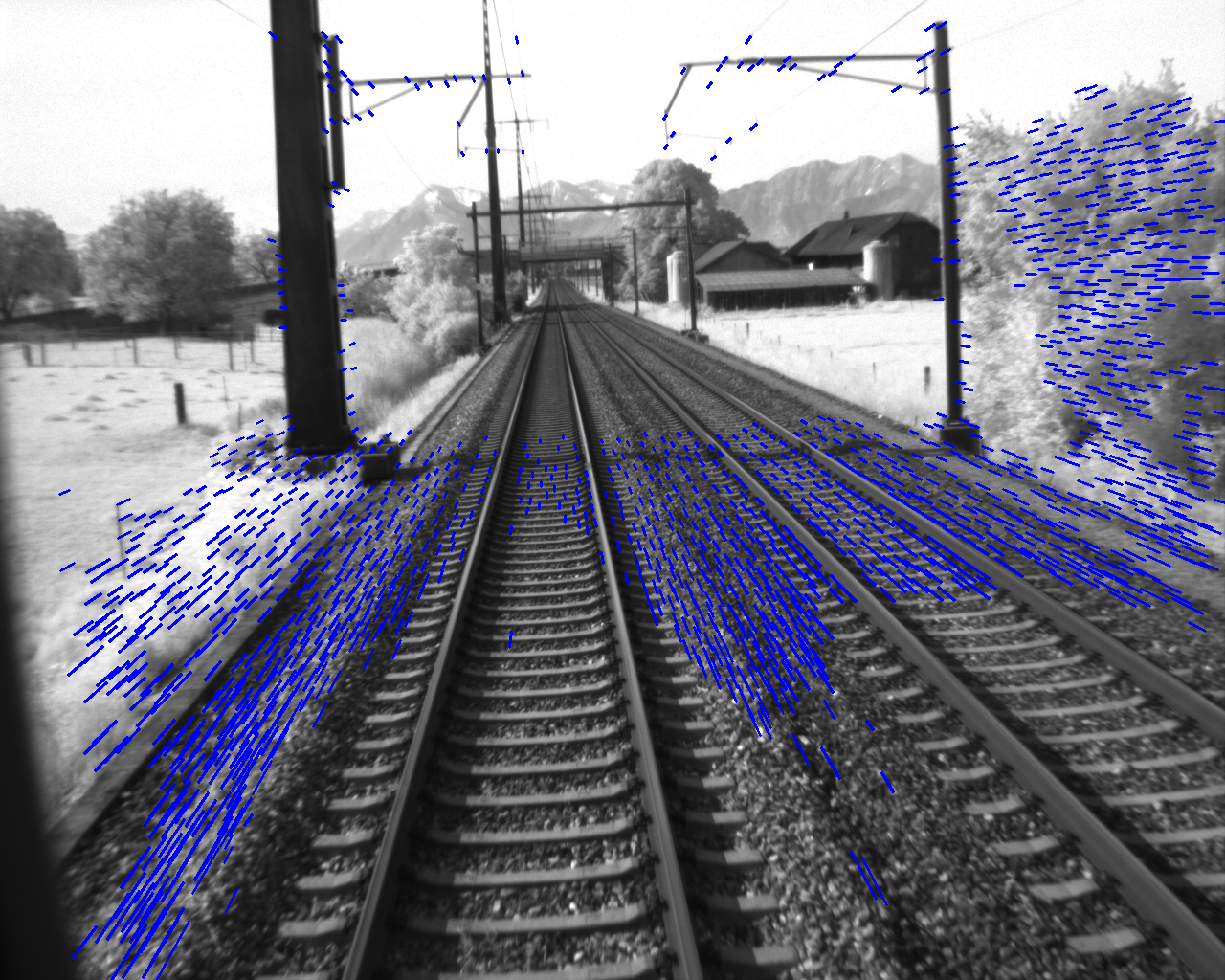
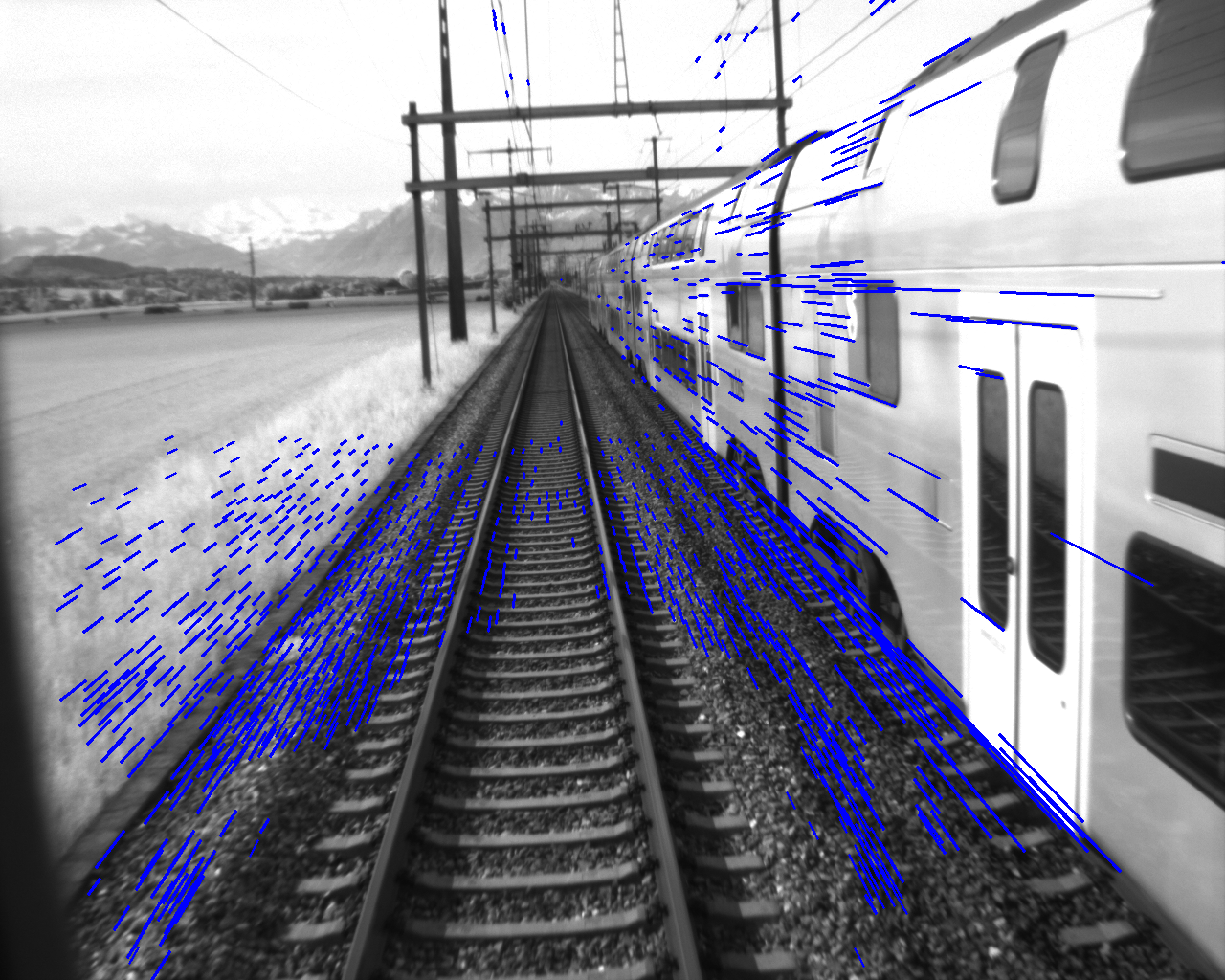
Figure 1: Strong dynamic occlusions in railroad scenarios: (left) tracking data in static environment; (right) navigation under strong dynamic occlusion

In order to be able to remove the additional track-side infrastructure, the precise and safe localization unit must be available on the vehicle. The challenge that requires additional research beyond the current state of the art method is that such a unit needs to provide verifiable results, which does not allow an application of Deep Learning methods and forbids even an application of standard methods, like RANSAC, due to its randomized processing with slightly varying results on same inputs. Additionally, the reliable static background information is limited only on the planar surfaces with highly self-similar, planar and repetitive structure of the gravel. This prevents applications of stereo-based system, which rely on clear 3D boundaries of planes, and of traditional sparse systems like ORBSlam, because the local features are not unique. It also requires powerful Future Railway Mobile Communication System (FRMCS) technology to monitor train integrity and send the exact position to the central interlocking. [5]. The development of localization is a decisive factor in the evolution of digitalization in the field of control and safety technology of railway systems. Additionally, the use of localization can also trigger a performance boost in today’s digital interlocking technology. With the integration of the new, precise localization technology, the operational performance of today’s control and safety technology can be increased in multiple domains. A standstill detection would make it possible to avoid track closures due to a lack of slip paths and thus achieve a more efficient use of the existing facilities. If today’s infrastructure- and odometry-based localization can be further developed into a continuous, object-side, autonomous SIL4 localization, enormous opportunities will open up for increasing efficiency and safety in a large number of railway applications.

We aim to make it possible to operate within the absolute braking distance in so called “Moving Blocks”. Consequently a more efficient handling of rail traffic is possible and leads to more track capacity on the very dense rail network used.

There are three main obstacles for the safe and precise localization of rail-bound vehicles:

1. Finding a sensor-combination and -fusion for a highly available, secure, safe and precise localization.

2. Obtain a SIL4 approval for the new localization system through the relevant certification bodies.

3. Secure interoperability within the European railways and setting international standardization.

The approach for localization described in this paper is only one out of several possible approaches that are taken into account in SmartRail 4.0.

I-A Rail-specific Navigation Problems

The applications for trains and rail infrastructure have to comply with highly-restrictive standards, like the CENELEC standards (EN 5012x, EN 50657), in order to be certified by the authorities. RAMS (Reliability, Availability, Maintainability, Safety) requirements have to be fulfilled to reach the required SIL (system integrity level). Therefore, safety critical applications such as a SIL 4 localization of track bound vehicles must be redundant (to reach availability) and need to meet diverse constraints in using deterministic algorithms (to reach safety level). Thus a use of machine learning or artificial intelligence approaches is not suitable for such systems. As we mentioned already earlier, the requirement to provide the same accurate measurement together with an information about the achieved accuracy from a specific image set, does not allow to use any probabilistic methods. It prohibits even the use of common techniques, like RANSAC, for model verification.

I-B Related Work

Optical navigation systems can be categorized based on the input data that they rely on. There exist many commercial systems [2, 16] that provide optical navigation data from 3D reconstructions in a binocular camera or camera-projector system. These approaches require static 3D structures like trees, houses or other objects in the scene that can be tracked over time. There are active 3D navigation systems mostly for door navigation, like RealSense camera, and outdoor binocular stereo systems, like ZED. As we can see in Fig. 1 such systems fail occasionally in the specific application field of a railroad scenario, because the strong occlusions by other trains passing on parallel tracks limit the available data to just the track bed in front of the train. The other type of navigation systems rely on the image information itself and can be subdivided in dense systems using the information of every pixel in the image [4] or matching significant points representing strong multi-directional brightness changes in the image [6, 9]. We do not consider learning approaches in our framework, because the resulting navigation system needs to undergo a strict verification process to be applied on trains and the current learning approaches do not meet this requirement.

There exist many optical navigation frameworks developed for the field of service robotics [3, 1, 4] and for outdoor navigation [13, 1, 14]. These systems have in common that they rely on matching of local image information over a time-sequence of images that creates the so-called optical flow, which is analyzed for its rotational and translational effects [6]. These approaches fail in many situations in railroad environments, because of the strong self-similarity of structures in the track bed, which is often the only reliable reference to the static environment. This required us to develop a different matching system that copes with this unstructured, repetitive property of the environment. It is presented in Section II-A.

Current monocular or stereo systems when applied on trains also suffer from the unstructured, repetitive environment, drifting gains and from aliasing to due the limited frame rate (20fps) at a max speed of 52,4 km/h [17]. In addition scenarios with other dynamic objects like cars and other trams or fast switching between shadow and sunlight limits the system performance in  [17]. Internal projects at SBB used cameras of maintenance vehicles to identify landmarks on or close to the track (e.g. balises, signs). However they are using machine learning algorithms which cannot be applied on safety critical applications like train localization. Due to the high RAMS requirements most of such vision based systems are applied as assistance systems only, today, even if autonomous driving would be the final goal [7]. The tram driver still has to override such assistance systems in order to avoid unnecessary emergency braking. Applying navigation assistance systems from the automotive domain fails due to the different environment and safety cases in rail. Odometry supported by wheel encoder like those used in automotive suffer from the high slip of rail vehicles (modern locomotives drive intentionally with slip.)

Many of the available systems are not able to provide any additional information about the quality of the currently estimated pose change of the camera. If the result is supposed to be fused in a fusion framework like a Kalman-Filter then the resulting covariance needs to be kept at a constant, worst-case level. We propose to extend the navigation approaches to provide the current uncertainty in the estimation of the pose in parallel to the navigation information. The accuracy may strongly vary based on the distance to the observed objects and their distribution in the camera image. The extension based on our work in [12] allows to estimate the quality of the processing (QoS) for each navigation step enabling a better convergence of the fusion framework. The proposed processing is described in Section II-B in more detail.

We present our approach, how to estimate the motion properties in Section II-B. Section II-A presents our approach, how to estimate robustly the metric motion of the camera in the highly unstructured area of the track bed. The possible drifts of the presented system are compensated through occasional information from global infrastructure, which is presented in Section II-B.We present in Section III the achieved accuracy in the motion estimation and metric measurements. We conclude with some final evaluation of the achieved system properties and discuss our further directions in Section IV.

II Approach

Visual localization provides information about motion of the camera relative to structures in the surrounding environment through direct observation of the changes in their projected position in the images. This prevents accumulation of position and orientation errors as long as the same global features can be kept visible. The position is extracted through processing of the image information and the pose (position and orientation) change is calculated with frame-rates in the range of 30-120Hz. This frequency limits the maximal possible dynamic motion of the system to changes occurring with a frequency smaller than half of that frame-rate.

In contrast, sensors like inertial units (IMUs) rely solely on physical effects within the sensor as a response to applied velocities and accelerations. They provide a significantly higher measurement rate, which can reach for an inertial unit values around 800-1000Hz. Small errors in the estimate due to noise or external disturbance cannot be compensated here through a global reference. They cause drifts that are accumulated during the integration of the consecutive measurements. A visual system exposes similar errors but with a significantly slower frequency, when a reference used to measure the current position needs to be changed to a new landmark (hand-off problem) [11].

We can see in Fig. 1 that the reliable area of the tracks that can be used for navigation does not provide unique matches in the tracking system that provides the information about the motion of the train. Local matching strategies that work reliably for flying systems and in the automotive domain cannot be applied in railroad environments due to this strong self-similarity of the local features.

We propose a final system architecture depicted in Fig. 2 to solve this problem. The navigation unit fuses the information from a point-based structure-from-motion (SfM unit - Section II-B) with a unit correlating large areas of the tracks to estimate robustly the metric motion of the train (correlation unit). The dynamic motion state of the train is currently estimated only from fusion of the optical unit with the Kalman Filter prediction. We plan to extend it with the information provided by an additional inertial unit (IMU) to allow capture of higher dynamic motions of lighter train setups.

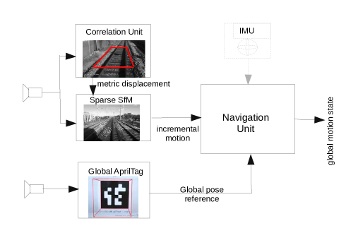
Figure 2: System architecture of the planned goal navigation system.(SfM: Structure from Motion)

Our system is calculating the pose changes from a monocular image sequence. This sequence is passed to a correlation unit that estimates the metric translational motion of the train from the motion of an image template in the track area between the images of the sequence. The details of the processing are presented in Section II-A in more detail. The rotational parameters and the direction of motion is calculated from a modified SfM module, where additionally the accuracy of the current navigation result is estimated. It is important for correct fusion in the Fusion Unit and for the planned certification of the system. This processing is presented in Section II-B.

The presented system cannot avoid long term drifts, because the correlation unit and the SfM module rely only on local features that can be used as reference only in limited space. Our system uses an additional long focal length camera that identifies April-Tags [15] placed instead of the usual identifiers along the track. These tags are used to compensate possible drifts in the navigation unit. They provide geo-tagged information about the position of the train in the world.

The navigation unit (Fig. 2) can further optimize the calculation of the distance by freezing the reference frame $\cal{I^{\prime}_{t}}$ (key-frame) for a number of following frames, if the estimated velocity is slow. Since the distance travel is the integral of the responses from the optical correlation, small detection errors usually integrate to increasing drifts in the distance. Switching to the key-frame-processing results in the detection errors appearing as noise overlayed over the true distance instead of appearing as accumulated drift (Section III-A).

II-A Robust Estimation of Metric Motion Parameters

Conventional Visual SLAM approaches use the information from a sparse point matching system in the camera images. The points are tracked between the image pairs from the sequence or matched based on the local information in the neighborhood of the points. The difference is that while tracking assumes a local search around the expected position, in which a local image patch is searched, matching allows larger changes in the image position, because each point is described by a more or less complex description (SIFT [8], AGAST [10]).

While this processing works in most flying and automotive environments, we need to be able to match the information in the area of the tracks with a very strong self similarity that leads to many mismatches between the frames. We increase the uniqueness of the local environment by growing the local region to a large area shown in the Fig. 3. We try to match this template in the consecutive image using a Sum-of-Square-Differences (SSD) method from OpenCV. We refer to this module because of the similarity to an optical computer mouse as “Train Mouse”.

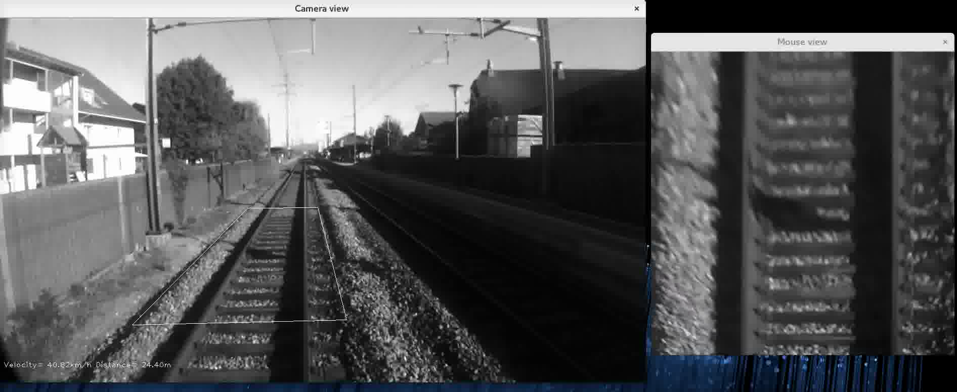
Figure 3: The rectangular region shown in the left image is rectified to the “top-view” image shown on the right. A template in this image is searched in the consecutive image rectified in the same way.

A homography matrix $\tilde{H}$ that is used to calculate the rectified image $\cal{I^{\prime}}$ in Fig. 3 right has the generic structure (1):

$$\tilde{H}=\left(\tilde{R}+\frac{\vec{T}\vec{n}^{T}}{d}\right)\quad\rightarrow\quad\cal{I^{\prime}}=\tilde{H}\cdot\cal{I}$$ (1)

The rotation matrix $\tilde{R}$ describes the rotation between the current orientation of the physical camera and the top-view orientation of the rectified view. The vector $\vec{T}$ describes the translation between the images, which is zero in our case. Therefore, plane normal vector $\vec{n}$ of the tracks and the distance of the camera to the tracks $d$ become irrelevant here. We use the homography to rotate the camera image $\cal{I}$ to the top-view $\cal{I^{\prime}}$ orientation.

We search for a rectangular template with the size $(x^{\prime},y^{\prime})$ from the ${\cal{I^{\prime}}}_{t}$ region of the first image in the corresponding region ${\cal{I^{\prime}}}_{t+1}$ using the SSD template matching method that searches for the maximum of the function (2):

$$f(x_{p},y_{p})=\sum_{x^{\prime},y^{\prime}}({\cal{I^{\prime}}}_{t}(x^{\prime},y^{\prime})-{\cal{I^{\prime}}}_{t+1}(x_{p}+x^{\prime},y_{p}+y^{\prime}))^{2}$$ (2)

The estimated displacement $(x_{p},y_{p})_{t}$ from the maximum response of $f(x_{p},y_{p})$ estimates the horizontal and vertical image motion of the template between the images. This measures a pixel accurate shift of the template between the images. The search for the correct displacement for the current $(x_{p},y_{p})_{t}$ can be accelerated by using a prediction of these values. In a generic case, the system needs to check the entire possible range of $\{x_{p},y_{p}\}$ that covers the entire possible velocity profile. This is a computationally intensive operation. Due to the high inertia of the train, these value change only little between consecutive frames. We can reduce the search for the correct placement of the template only to a small band around the previous $(x_{p},y_{p})_{t-1}$ values.

We can calculate a more accurate displacement of the template between the images by applying a sub-pixel alignment of the templates. If the remaining change between both images is under 1 $\left[\mbox{pixel}\right]$ then we can use the Taylor series expansion to explain the brightness change at a specific pixel ${\cal{I^{\prime}}}(x,y)$ to:

$${\cal{I^{\prime}}}_{t}(x+\delta x.y+\delta y)\approx$$ (3)

$${\cal{I^{\prime}}}_{t}(x,y)+\frac{\partial{\cal{I^{\prime}}}_{t}(x,y)}{\partial x}\delta x+\frac{\partial{\cal{I^{\prime}}}_{t}(x,y)}{\partial y}\delta x$$

If we assume that the new image ${\cal{I^{\prime}}}_{t+1}$ is a result of a sub-pixel motion $(\delta x,\delta y)$ then we can estimate from the equation:

$${\cal{I^{\prime}}}_{t+1}(x.y)-{\cal{I^{\prime}}}_{t}(x,y)\approx$$

$$\frac{\partial{\cal{I^{\prime}}}_{t}(x,y)}{\partial x}\delta x+\frac{\partial{\cal{I^{\prime}}}_{t}(x,y)}{\partial y}\delta x=\vec{\cal{G}}^{T}\cdot\delta\vec{p}=||\vec{\cal{G}}||\cdot||\delta\vec{p}||$$ (4)

$$\mbox{with}\quad\vec{\cal{G}}=\left(\frac{\partial{\cal{I^{\prime}}}_{t}(x,y)}{\partial x},\frac{\partial{\cal{I^{\prime}}}_{t}(x,y)}{\partial y}\right)^{T}$$

We see that once we calculated the gradient vector ${\cal{G}}$ from the previous image, we can calculate the sub-pixel update of the motion in horizontal and vertical direction $(\delta x.\delta y)$ by decomposing the motion $||\vec{\delta p}||$ along the gradient according to the horizontal and vertical ratios of $\vec{\cal{G}}$.

We calculate the resulting shift as an average of responses within the template. It is obvious from (4) that only pixels with a difference in brightness between the images contribute to the motion estimation. We reduce the sensitivity to noise by using only pixels with the gradient above a threshold $||\vec{\cal{G}}||>\epsilon_{G}$, which is tuned depending on the expected camera noise.

The resulting average image motion $(\Delta x,\Delta y)$ can be linearly scaled to the forward and side-wards metric velocity with knowledge about the mounting height L above the ground. The metric values of the forward velocity $v_{l}$ and the side-wards motion $v_{s}$ (due to curves in the route) can be computed from similar triangles relation between the camera projection on the image plane and the relation of the height L of a rectified camera providing the image $\cal{I^{\prime}}$ to:

$$\Delta x_{i}=x_{p}+\delta x,\quad\Delta y_{i}=y_{p}+\delta y$$

$$v_{l}=\frac{L\cdot p_{y}}{f\cdot t_{f}}\Delta y_{i},\quad v_{s}=\frac{L\cdot p_{x}}{f\cdot t_{f}}\Delta x_{i}$$ (5)

Possible changes in the orientation of the camera image $\cal{I^{\prime}}$ scale it with the focal length $f$, the metric pixel-size $(p_{x},p_{y})$ and the time interval between two frames $t_{f}$ as it is shown in (5). The improvement achieved with the extension to the sub-pixel accuracy is shown in Section III-A.

A possible error in the estimate of the traveled global distance $(x_{g},y_{g})$ can occur due to the noise in the brightness information ${\cal{I^{\prime}}}_{t}(x,y)+\nu_{i}$. Since the global shift is an integral (sum) of the consecutive steps $(\Delta x,\Delta y)$, the error accumulates fast in each step. The resulting shift in each step is estimated as an average response of all significant brightness changes within the templates. The statistical distribution of the error helps to reduce the error in the final estimates. This can be pushed even further by tracking a template not only between consecutive images but over a longer period of time. The reference template from the original image, which we will refer to as keyframe in the following text, is used to estimate the shift in multiple following frames. It is done until the template moves out from the area warped in the convolution step above. This processing introduces the brightness noise-related error only once in the navigation process, instead of being added multiple times with each new delta step. The length of the sequence, in which a keyframe can be used, depends directly on the current speed of the train. We will see in Section II-B that this processing has an additional advantage on the motion estimation process.

A significant advantage of adding a separate estimation of the forward motion is the possibility of estimation of the typically unobservable motion error $\sigma_{z}$ along the optical axis Z. We are able to estimate this error from the $\Delta y_{i}$ responses of all N contributing pixels in the template with the property $||{\cal{G}}||>\epsilon_{G}$ to:

$$\sigma_{z}^{2}=\frac{1}{N}\sum_{i\in||\vec{\cal{G}}||>\epsilon_{G}}(\Delta y_{i}-\overline{\Delta y})^{2},\;\overline{\Delta y}=\frac{1}{N}\sum_{i\in||\vec{\cal{G}}||>\epsilon_{G}}\Delta y_{i}$$ (6)

II-B Robust Key-frame-based Monocular Motion Estimation

The keyframe processing introduced in the previous section improves also the accuracy of the estimation of the direction of motion in the monocular Essential matrix decomposition [6]. Our problem with the matching of features between images of the sequence is the significant self-similarity of the observed features (Fig. 4). Typical matching algorithms like SURF, BRISK, KAZE, find multiple matching candidates for a tracked point.

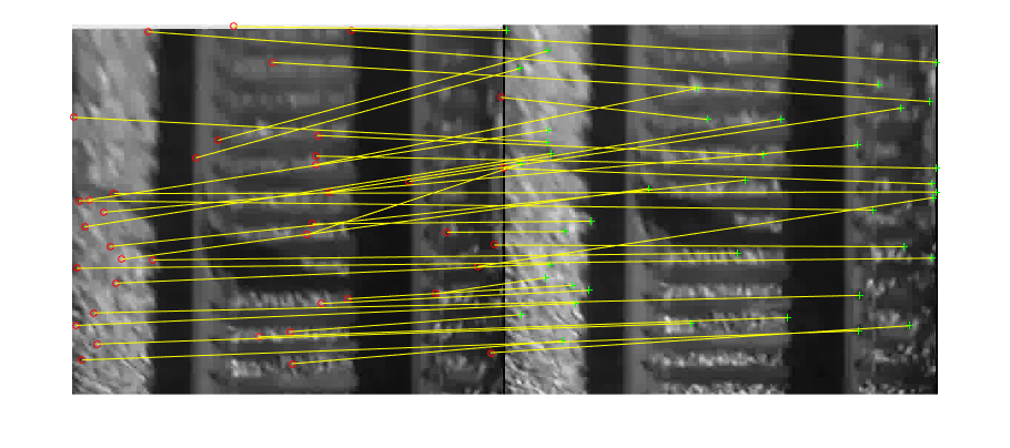
Figure 4: Strongest matching candidates are often not the correct correspondences for feature points in track area.

The selection of the correct matching candidate can be largely simplified. Since the previous optical correlation step found the planar direction of motion, which represents the first $T_{x}$ and the last $T_{z}$ parameters of the motion vector, we can estimate the horizontal position of the epipole in the image. The direction of the motion vector $\vec{T}$ defines the position of the intersection point of all optical flow lines, which are segments of the corresponding epipolar lines (see Fig. 5).

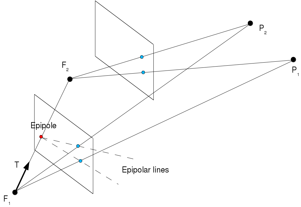
Figure 5: While the camera is moving along the vector $\vec{T}$, the tracked points move along the dashed epipolar lines in the second image frame.

Our system uses the predicted value for the rotation matrix R that is calculated in the fusion framework of the Navigation Unit (Fig. 2). We rotate all matched points $\vec{p_{i}}=(u_{i},v_{i},f)^{T}$ by this matrix to a rotation compensated version $\vec{p}^{\prime}_{i}$:

$$\vec{l}=\tilde{R}^{T}\cdot\vec{p_{i}},\quad\underline{\vec{p}^{\prime}_{i}=\frac{f}{l_{z}}\cdot\vec{l}}$$ (7)

The resulting optical flow has just the translational component, which intersects in the expected epipole. Since the rotation is just a prediction, we allow the optical flow lines to deviate by a small pixel value from this epipole. An example for the compensated optical flow field can be found in Fig. 1. We choose the matches from the matching pool, which point towards the expected epipole.

Once the correct matches between features in both images are found, we estimate the new corrected $\tilde{R}$ and the direction of motion vector $\vec{T}$ using processing similar to standard calc_pose() method from OpenCV without the RANSAC part. The filtering was done before in a deterministic way. The proposed novelty is the way, how we additionally filter the wrong correspondences based on the expected epipole above. The solution becomes ambiguous especially in strongly limited visible space without this processing.

An important final step in the processing is the calculation of the covariance of the result. We estimated the metric $\sigma_{z}$ component already in (6). We estimate the remaining two components by estimating the distances, how far the lines associated with the flow segment miss the epipole. For an i-th flow vector with start and end-point $(\vec{p}_{si},\vec{p}_{ei})$, we can estimate the epipole point $\vec{x}_{e}$ to:

$$\vec{k}_{i}=\left(\begin{array}[]{c}k_{u}\\ k_{v}\end{array}\right)=\vec{p}_{ei}-\vec{p}_{si},\quad\vec{n}_{i}=\left(\begin{array}[]{c}-k_{v}\\ k_{u}\end{array}\right)$$ (12)

$$\tilde{A}=\left(\begin{array}[]{c}\vec{n}_{1}^{T}\\ .\\ .\\ \vec{n}_{k}^{T}\end{array}\right),\quad\vec{b}^{T}=\tilde{A}\cdot\left(\vec{p}_{s1},\dots,\vec{p}_{sk}\right),\quad\underline{\tilde{A}\cdot\vec{x}_{e}=\vec{b}}$$ (17)

The epipole position $\vec{x}_{e}$ can be estimated using a pseudo-inverse of the non-square matrix $\tilde{A}$ in (17). An essential information for a fusion in the Navigation Unit is the covariance of the estimated value. It helps to assess the current uncertainty in the measurement. We calculate the closest distance $\vec{\delta p}_{i}$ for flow optical flow-line $(\vec{p}_{si},\vec{p}_{ei})$ from $\vec{x}_{e}$ using $\Delta x$ result from (5) for a scaling from pixel-values to meters as:

$$\vec{\delta_{p}}_{i}=\frac{\Delta x\cdot p_{x}}{f}\left[\vec{n}_{i}^{T}\cdot\left(\vec{x}_{si}-\vec{x}_{e}\right)\right]\cdot\vec{n}_{i}$$ (18)

The resulting covariance matrix $\tilde{P}$ in the xy-plane from k optical flow lines is constructed as:

$$\tilde{P}=\frac{1}{k}\sum_{i=1}^{k}\vec{\delta_{p}}_{i}\cdot\vec{\delta_{p}}_{i}^{T}$$ (19)

The keyframe processing helps similar to the previous chapter to reduce the error while switching to new references by significantly reducing the number of switches. Additionally, the flow line-segments in the images become longer. If we assume a constant detection error for the flow endpoints in the images then longer lines are less sensitive to orientation changes due to the detection error.

II-C Drift Compensation from Global Landmarks

Since (visual) odometry or IMUs only provide a relative localization, global landmarks are required for getting world coordinates. These relative algorithms also suffer from an accumulative offset and an unknown initial condition of the real value that leads to a drift from the real position. To compensate for that drift other sensors needs to be included in the sensor system. Using GNSS is the most promising approach, however in areas without GNSS coverage (e.g. in tunnels or valleys) another approach could be helpful. As such an alternative vision based solutions such as April tags (or similar tags or signs) mounted on the poles of the catenary, whose position is known in world coordinates with an accuracy within 10 cm, can be successfully used. The global pose of the camera relative to the tags can be easily derived. Further vision based approaches could be using other global and fixed landmarks of the environment (e.g. points).

III Experimental Results

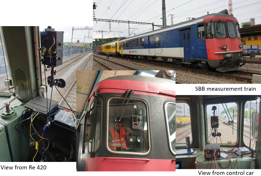
Figure 6: SBB measurement train and camera setup in locomotive (Re 420) and control car

The setup up for the trial was a specific train run organized by SBB where cameras were installed on the windscreens of the locomotive and the control car (see Fig. 6). There were two cameras each, one for the “Train Mouse” and one for the April tags mounted on the poles for the catenary. The 10 bit NIR cameras with a resolution of 1280 by 1024 pixels were used at a frame rate of 60 fps. The cameras were supported by IR-illuminators to overcome tunnels. All camera were calibrated using the Bouquet toolbox with a 9x6 checkerboard with 8cm by 8cm tile size. The SBB telecom measurement wagon in the middle of the train composition provided the position reference as it was equipped with a DGNSS solution combined with an IMU (high performance ring-laser gyro). The approx. 20 minutes trip between Ostermundigen and Thun were repeated four times in order to reproduce results with different speeds up to 140 km/h and different scenarios (e.g. occlusion by other trains). This route was chosen because it also contains the 8km long fiber optic sensing (FOS) test track and enabled a comparison of the results of the different localization sensors. The route consists mostly of two parallel tracks and 4 railway station were there are several points and up to 6 parallel tracks.

III-A Accuracy of the Correlation Approach (“Train Mouse”)

Fig. 7 depicts the necessity to include the sub-pixel motion estimation into the metric motion estimation system. This allows an early notification about the train setting in motion even before the human eye can observe it. It is also very important at higher velocities, where a change of one pixel in motion between 2 frames corresponds to multiple km/h at typical speeds of up to 140km/h.

Figure 7: Comparison between velocity estimation without (blue) and with (red) sub-pixel optimization.

The optical correlation system (“Train Mouse”) achieves an accuracy beyond the capabilities of the existing mechanical and GNSS sensors (Fig. 7). It is possible to see small velocity changes, which can be used to analyze changes in the dynamic state of the train, if multiple units are distributed over the length of the train. We can observe changes, e.g. due to oscillations of the train control system, on the track. It is to our knowledge the first system in the rail domain operating at velocities equal or higher than 140 kmh because of successful solution of the matching problem through correlation.

The estimated profiles tracked over one of our test runs are depicted in Fig. 8. The tracked velocity was confirmed with GNSS measurements in areas, where the GNSS reception was available. We show the comparison in Fig. 8middle.

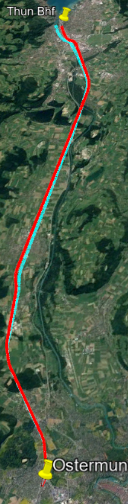
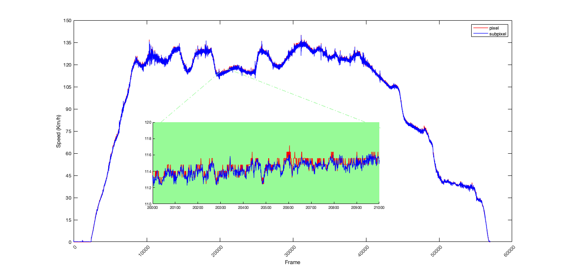
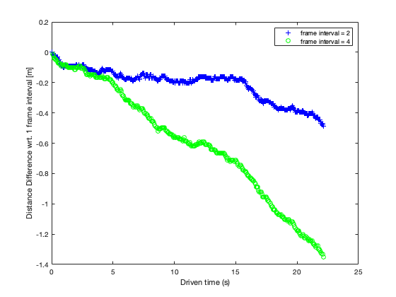
Figure 8: (Left) Overlay of estimated route (blue) and GPS estimate(red);(middle)Velocity plot from the Optical Correlation (“Train Mouse”) Module. The steps due to the pixel quantization show the necessity for sub-pixel processing (blue) compared to pixel-accurate SSD only method (red); (right) Reduction of the drift accumulation through longer keyframe sequences in optical correlation (“Train Mouse”).

The extension of the number of frames, in which the same template is tracked results in significant reduction of drifts (Fig. 8)right.

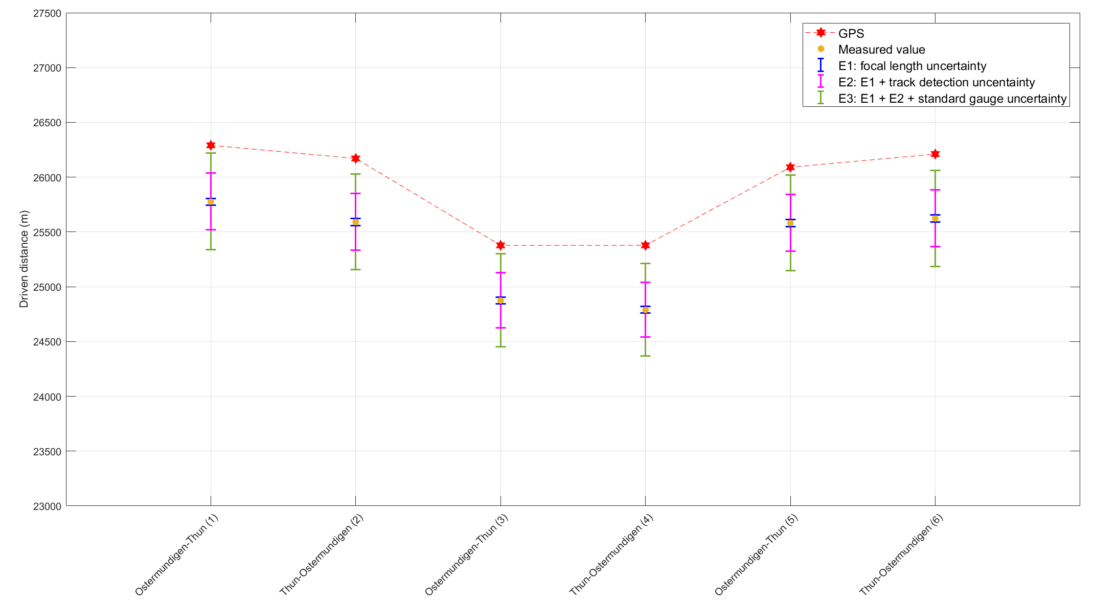
Figure 9: Agreement between the GPS measurement and distance estimated with “Train Mouse”.

The additional drift in accumulated over a distance of 855m was 0.84m for a system with 1/4 less reference frame switches. In 22 seconds the system made 30*22 switches for the (green) case of continuous reference updates and 15*22 switches for the (blue) case of a keyframe sequence length of 4. The decrease in the measured distance is -1.31m for the blue and 0.49m in the green case. We see that the blue curve traveled a shorter distance than the continuously switching case which corresponds to the zero line in Fig. 8right.

Fig. 9 shows a good estimate of the traveled distance compared to the GPS measurement based entirely on the “Train Mouse” without compensation with April-Tags. We see how different parameters, like focal length, height above the ground, and gauge distance influence the parameters. We currently work on on-line re-calibration of this error.

III-B Performance of the Motion Estimator

The system was run on a Quadcore Pentium i5 3.1GHz with an NVIDIA GTX1080 for low-level image processing. The system was able to do per-frame calculations in the range 07-11ms/frame, which allows online processing of the 60Hz image streams from the camera.

Fig. 10 shows the system processing along the route for the case of an open space and a curve motion. The map plotted in red next to the visualization window corresponds to the route form from the local region. The accuracy of this part of the processing was already successfully verified in [11]. Our current test was to see, how many optical flow vectors can explain the current motion of the train but passing the epipole not further than 0.5 pixels. The while line segments in Fig. 10 shows a very large number of such segments with a large spread over the image. This results in a very small drift in motion orientation [12].

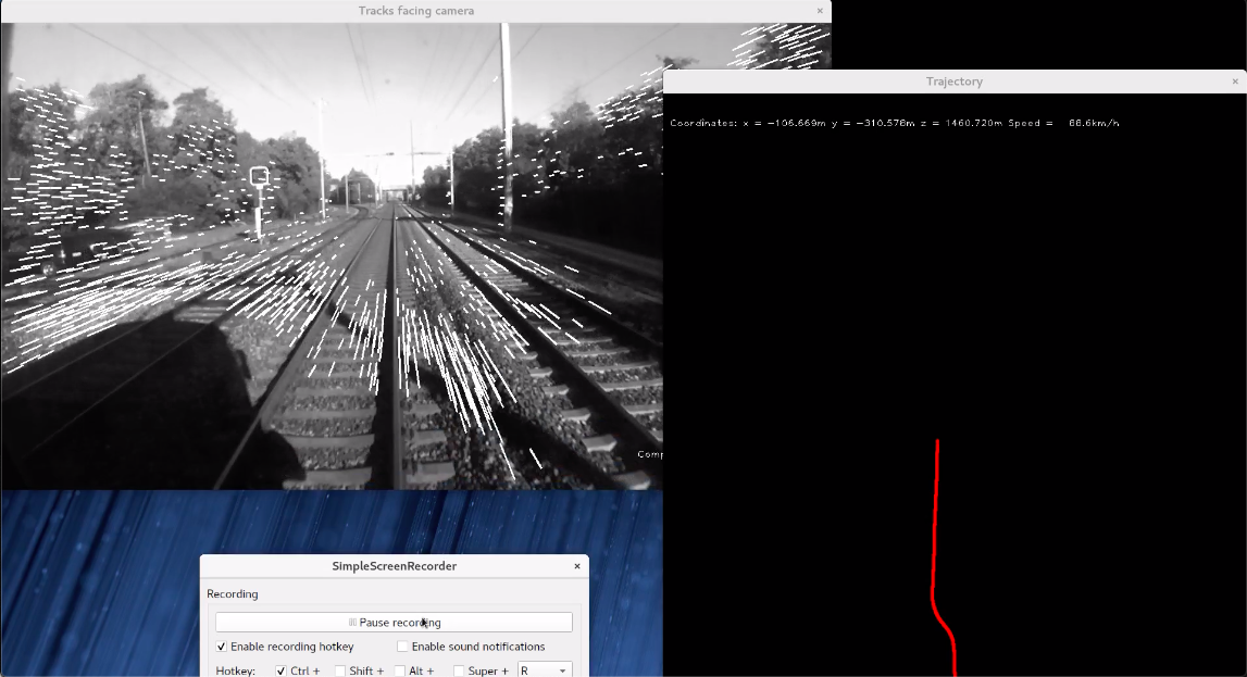
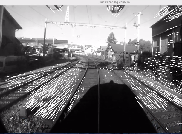
Figure 10: Real-time calculation of filtered flow for higher velocities (left) and curve motion (right).

We see in Fig. 10 that the epipole prediction from the computation in the Optical Correlation (“Train Mouse”) module can successfully be used to filter correct correspondences that capture the ego motion of the train with the point of expansion in the intersection point of the ego-velocity vector with the image plane (epipole).

In comparison to current system like the ones in  [17], we can keep up with speeds greater than 140 km/h. There is nearly no influence from other objects, since we only rely on a small track area in front of the rail vehicle. Using NIR cameras in our approach weakens the effect of shadows and sunlight. With the “train mouse” we derive the gain for the z-axis directly from the known track gauge width, avoiding gain drifts as in  [17].

III-C Fusion of Navigation Data from Global Landmarks

Using sensor fusion techniques (e.g. Kalman filtering based on a train model) the relative positions can be combined with the world coordinates thus effectively compensating for drift and filter off outliers and noise. Using an IMU together with the train model will provide even more robust results. In addition an accurate and trusted topological map of the tracks can be used to further improve accuracy and to determine the integrity of the position information.

Figure 11: Results of pose estimation for an April tag.

In Figure 11 the pose estimation results for a given April tag when passing by with the measurement train are shown. It can be seen that the perpendicular distance from the pole to the track (X) is nearly constant as well as the height (Y) while passing an April tag mounted on a pole of the catenary. The table shows the values for 9 consecutive image frames while the train covers a distance of approx. 5 m.

IV Conclusions and Future Work

We presented a system that represents an approach to deal with specific requirements of unstructured dynamic railroad scenarios. The system shown in Fig. 2 has a modular structure with modules that provide the dynamic motion updates with varying update rates and drift properties. In our current application, the train dynamics is slow enough due to the stiff suspension of the trains to observe the dynamics with the 60Hz update rate of our monocular camera system. We plan to extend it to more agile train suspensions that will require a faster dynamic update and an addition of an IMU unit shown in the Fig 2.

Our main contribution is three-fold:

Low-Level Matching under Strong Self-Smilarity

- we adapted the low-level vision unit to cope with the ambiguous world of the railroad environment with very strong self-similarity between the local objects (stones, screws, etc.). We extended the local descriptor to the entire track area under the planarity assumption for the track bed. This makes the matching system more robust. The vanishing points from the motion estimate allow also a robust filtering of correct landmarks for SfM module without any random selections as it is the case for RANSAC systems. This is an essential pre-requisite to be able to make the system verifiable for the SIL 4.0 requirements.

Calculation of Error Covariance

- our system calculates not only the current pose change but also the confidence of the result as a covariance matrix. This allows on one hand a better monitoring of the QoS (Quality of Service) but at the same time it improves essentially the convergence properties of the fusion network in the Navigation Unit (Fig. 2). The processing allows also weighing of the used optical flow vectors depending on their reliability (length in the image). This is our next step to improve the accuracy of the SfM module.

Key-frame Processing

- instead of a bundle-adjustment step common for most of the SLAM approaches, we apply the key-frame processing idea that reduces the number of reference changes during operation of the unit. The specific problem of railroad environments is the strong occlusions of distant features which requires to focus on the track-bed itself as navigation area. We currently compensate for drifts with artificial landmarks, e.g., April tags along the way, but we plan to use a system that will try to re-identify distant objects (once they come into view after a train pass again) that will also allow to compensate for the drift more efficiently.

With the above shown “optical navigation” the following properties were achieved for the visual sensors:

1. skid-free odometer (visual odometry) 2. “visual” balise (detecting April tags) 3. incremental motion 4. track selectivity 5. global pose reference in six dimensions (combined with a map) (visual localization) 6. real-time capability of the image processing @ 60 Hz

The “optical navigation” presented here has the advantage that it is deterministic and does not require machine learning algorithms (for example neural networks or deep learning). No SIL4 application based on machine learning has yet been approved by a relevant certification body. This “optical navigation” opens up the opportunity to provide evidence of a safe and secure image processing for the localization. Since the image processing can provide incremental motion as well as global pose reference it is a potential sensor for a safe sensor-fusion, but to guarantee diversity it must be combined with other sensors (for example IMU).

Interoperability within the European railways and setting international standardization has to be achieved, after the sensor-fusion is proven and the first approval through a relevant certification body was accomplished .

The data acquisition took place in a vision friendly environment with good weather conditions. Therefore dealing with worse weather conditions or other environments is beyond the scope of this paper and it will be focused on in the next steps.

References

- [1] Darius Burschka and Elmar Mair. Direct pose estimation with a monocular camera. In Robot Vision Workshop, Auckland, New Zealand, pages 440–453, 02 2008.
- [2] Intel Corp. Intel RealSense Technology. https://www.intel.com/content/www/us/en/architecture-and-technology/realsense-overview.html.
- [3] Andrew J. Davison, Ian D. Reid, Nicholas D. Molton, and Olivier Stasse. Monoslam: Real-time single camera slam. IEEE Trans. Pattern Analysis and Machine Intelligence, 29:2007, 2007.
- [4] Jakob Engel and Daniel Cremers. Lsd-slam: Large-scale direct monocular slam. In In ECCV, 2014.
- [5] Reto Germann. Accurate localisation - an ingenious approach. Signal+Draht (Signalling&Datacommunication), (7+8):3, 07 2019.
- [6] R. I. Hartley and A. Zisserman. Multiple View Geometry in Computer Vision. Cambridge University Press, ISBN: 0521540518, second edition, 2004.
- [7] Matthias Hofmann, Christian Klier, and Holger Last. The first autonomous tram - made by siemens. experiences and challenges of the research project with verkehrsbetrieb potsdam. In Tagung moderne Schienenfahrzeuge, 45. Tagung. Technische Universität Graz, April 2019.
- [8] David G. Lowe. Distinctive image features from scale-invariant keypoints. International Journal of Computer Vision, 60(2):91–110, 2004.
- [9] Elmar Mair and Darius Burschka. Mobile Robots Navigation, chapter Zinf - Monocular Localization Algorithm with Uncertainty Analysis for Outdoor Applications, pages 107–130. In-Tech, March 2010.
- [10] Elmar Mair, Gregory Hager, Darius Burschka, Michael Suppa, and Gerhard Hirzinger. Adaptive and generic corner detection based on the accelerated segment test. In European Conference on Computer Vision (ECCV 2010), 09 2010.
- [11] Elmar Mair, Klaus Strobl, Michael Suppa, and Darius Burschka. Efficient camera-based pose estimation for real-time applications. In 2009 IEEE/RSJ International Conference on Intelligent Robots and Systems, IROS 2009, 11 2009.
- [12] Elmar Mair, Michael Suppa, and Darius Burschka. Error Propagation in Monocular Navigation for Zinf Compared to Eightpoint Algorithm. In Proceedings of the IEEE/RSJ International Conference on Intelligent Robots and Systems (IROS’13), November 2013.
- [13] Christopher Mei, Gabe Sibley, Mark Cummins, Paul M. Newman, and Ian D. Reid. Rslam: A system for large-scale mapping in constant-time using stereo. International Journal of Computer Vision, 94:198–214, 09 2011.
- [14] Raul Mur-Artal, J Montiel, and Juan Tardos. ORB-SLAM: a versatile and accurate monocular SLAM system. IEEE Transactions on Robotics, 31:1147 – 1163, 10 2015.
- [15] University of Michigan. AprilTags. https://april.eecs.umich.edu/software/apriltag.
- [16] StereoLabs. ZED Camera. https://www.stereolabs.com/zed/.
- [17] Florian Tschopp, Thomas Schneider, Andre W. Palmer, Navid Nourani-Vatani, Cesar Cadena, Roland Siegwart, and Juan Nieto. Experimental comparison of visual-aided odometry methods for rail vehicles. In IEEE Robotics and Automation Letters, Vol. 4, No. 2, pages 1815–1822. IEEE Computer Society, April 2019.