Search for Alignment of Disk Orientations in Nearby Star-Forming Regions: Lupus, Taurus, Upper Scorpius, $\rho$ Ophiuchi, and Orion

Abstract

Spatial correlations among proto-planetary disk orientations carry unique information on physics of multiple star formation processes. We select five nearby star-forming regions that comprise a number of proto-planetary disks with spatially-resolved images with ALMA and HST, and search for the mutual alignment of the disk axes. Specifically, we apply the Kuiper test to examine the statistical uniformity of the position angle (PA: the angle of the major axis of the projected disk ellipse measured counter-clockwise from the north) distribution. The disks located in the star-forming regions, except the Lupus clouds, do not show any signature of the alignment, supporting the random orientation. Rotational axes of 16 disks with spectroscopic measurement of PA in the Lupus III cloud, a sub-region of the Lupus field, however, exhibit a weak and possible departure from the random distribution at a $2\sigma$ level, and the inclination angles of the 16 disks are not uniform as well. Furthermore, the mean direction of the disk PAs in the Lupus III cloud is parallel to the direction of its filament structure, and approximately perpendicular to the magnetic field direction. We also confirm the robustness of the estimated PAs in the Lupus clouds by comparing the different observations and estimators based on three different methods including sparse modeling. The absence of the significant alignment of the disk orientation is consistent with the turbulent origin of the disk angular momentum. Further observations are required to confirm/falsify the possible disk alignment in the Lupus III cloud.

1 Introduction

Stars are the fundamental building blocks of the visible universe, and their formation and evolution are among the most important areas of research in astronomy. It is well-known that multiple star formation is commonly observed in star forming regions (e.g. Lada & Lada, 2003), and also that more than half of stars at present with stellar masses larger than the Solar mass form binary systems (e.g. Duchêne & Kraus, 2013). Nevertheless, details of the multiple star formation process are not yet well understood theoretically despite numerous previous efforts (e.g Krumholz, 2014).

The distribution of the stellar spin and/or proto-planetary disk rotation, or “alignment” among stellar angular momenta, may retain unique information on the physics of star formation. For instance, if multiple disks form through collapse and fragmentation of a rotating primordial molecular cloud, they would somehow inherit the initial angular momentum of the cloud, and share the direction of the original rotation. If the turbulence in the cloud dominates its global rotation, however, the disk rotation axes are significantly perturbed and would be randomly distributed. The presence of magnetic field further complicates the situation. If a primordial cloud has a coherent strong magnetic field, its gravitational collapse preferentially proceeds along the magnetic field. Thus the rotational axes of disks formed out of the cloud would be aligned with the direction of the magnetic field.

The above different pictures have been studied with hydrodynamical simulations without magnetic fields by tracking the evolution of a collapsing molecular cloud. Specifically, Corsaro et al. (2017) showed that the strong spin alignment is realized if the initial rotational energy of the proto-cluster is significant. In addition, Rey-Raposo & Read (2018) confirmed the spin alignment for the proto-cluster, whose initial condition is taken from a larger disc-galaxy simulation. In reality, however, the competition among the global rotation, turbulence and magnetic field in real star-forming regions is much more complex, and needs to be unveiled individually from the precise observational data.

There are several attempts to search for the alignment among the spin directions of (proto)stars in star forming regions and star clusters, but their claims are not conclusive and sometimes even confusing. Corsaro et al. (2017) measured the stellar inclination, $i_{\rm s}$, of 48 red giants in two open clusters using asteroseismology, and claimed that both regions show strong alignment (over $6\sigma$ and $5\sigma$, respectively), while Mosser et al. (2018) did not find such alignment from their reanalysis of the same data. Jackson & Jeffries (2010) found no statistical trend of the alignment of stellar spins in Pleiades and Alpha Per clusters from $i_{\rm s}$ estimated jointly by spectroscopic projected stellar rotational velocity $v_{\star}\sin i_{\rm s}$, the photometric stellar rotation period $P_{\rm rot}$, and the stellar radius $R_{\star}$. Jackson et al. (2018) also reconfirmed that there is no strong evidence of the alignment among stars in Pleiades. More recently, however, Kovacs (2018) reported evidence for alignment of stellar spins in the open cluster, Praesepe, from $i_{\rm s}$ based on the same technique. On the other hand, Stephens et al. (2017) reported that outflows, which are expected to indicate the direction of the stellar spin, in the Perseus molecular cloud are randomly oriented in reality.

In addition to those somewhat confusing observational results, the stellar spin may not be a good proxy of the rotation direction of the disk since the amplitude of the stellar spin is significantly smaller than that of the disk angular momentum, and could be affected more easily by other local processes. For instance, the strong diversity of the spin-orbit architecture is well established in exo-planetary systems (e.g. Winn & Fabrycky, 2015). In particular, Kepler-56 is a transiting multi-planetary system exhibiting a significantly oblique stellar spin; Huber et al. (2013) discovered that its stellar inclination angle $i_{\rm s}$ is about 45 degree from the asteroseismic analysis. While it is not clear if the misalignment is of primordial or dynamical origin, this indicates a possibility that the stellar spin and disk rotation axes are significantly different. Furthermore, it would be more difficult to identify directions of stellar spins embedded in disks or envelopes. In addition, the directions of outflows could change from large to small scales, implying that the they might not be good tracers of the stellar spins (Bussmann et al., 2007).

Therefore the physics of star formation may be more likely to be imprinted in the degree of the alignment of proto-planetary disk orientations, rather than that of stellar spins. This is why we attempt the systematic analysis of the axes of spatially resolved disks and their correlations in five near-by star-forming regions; Lupus, Taurus, Upper Scorpius, $\rho$ Ophiuchi, and Orion.

The rest of the paper is organized as follows. Section 2 describes the statistical analysis of the alignment among disks in this paper. Specifically, we adopt the Kuiper test to check the departure from the uniform distribution of the position angles (PA) of disks. Section 3 summarizes our target star-forming regions and their observations. Section 4 presents our main result that the disks in star-forming regions are consistent with the random orientation except the Lupus III cloud that indicates the departure from the random distribution at 2$\sigma$ level. In Section 5, we examine the robustness of the derived values of PAs in the Lupus clouds using different data and estimators including a sparse modeling method. The implications of the present result are discussed in Section 6, and Section 7 is devoted to the conclusion. Finally we present the details of our sparse modeling analysis in Appendix A.

2 Statistical analysis of the position angle and inclination of the disks

Given the projected image of a disk, one can approximate it by an ellipse and estimate its position angle, PA, and inclination, $i$, relative to our line-of-sight. Specifically, PA refers to the angle of the major axis measured counter-clockwise from the north. Since we assume that the disk is circular in reality, $\cos$ $i$ should be equal to the ratio of the minor and major axes of the ellipse; the face-on and edge-on disks correspond to $i=0^{\circ}$ and $i=90^{\circ}$, respectively. Note we consider the range of PA and $i$ as $0^{\circ}\leq{\rm PA}<180^{\circ}$ and $0^{\circ}\leq i<90^{\circ}$ since the ellipse fit alone cannot distinguish between PA and ${\rm PA}+180^{\circ}$ and between $i$ and $180^{\circ}-i$. In the case that the additional spectroscopic data are available (for instance the Lupus III region below), one can break the degeneracy between PA and ${\rm PA}+180^{\circ}$, and estimate PA for $0^{\circ}\leq{\rm PA}<360^{\circ}$.

Since the disk inclination may change the detection threshold of the disk, its correlation might suffer from the selection bias; for instance, the observed flux of an optically-thick disk is proportional to $\cos i$, which preferentially increases the fraction of face-one disks with $i\approx 0^{\circ}$. Thus we mainly use the observed distribution of PA in order to test the possible correlation of the disk orientation. When we identify a signature of correlation in the PA distribution for a particular star-forming region, however, we consider the distribution of $i$ as well to see if it exhibits a similar non-uniformity.

Due to the degeneracy of the value of PA mentioned above, a widely-used statistics to validate the non-uniformity of the distribution, the Kolmogorov-Smirnov test for instance, cannot be applied in a straightforward fashion. Therefore we adopt a statistics proposed by Kuiper (1960), which improves the KS test for variables with rotational invariance. In the present case, the Kuiper test evaluates the difference of the two cumulative distributions using the following statistics:

$$D=\max_{\scriptscriptstyle 1\leq n\leq N}[F_{\rm ref}({\rm PA}_{n})-F_{\rm obs}({\rm PA}_{n})]+\max_{\scriptscriptstyle 1\leq n\leq N}[F_{\rm obs}({\rm PA}_{n})-F_{\rm ref}({\rm PA}_{n})],$$ (1)

where PA_n denotes the position angle of the $n$-th disk ($1\leq n\leq N$), $F_{\rm ref}$ is the reference cumulative distribution, and $F_{\rm obs}$ is the empirical cumulative distribution of the observed data.

If we take the reference distribution to be uniform, the non-uniformity can be evaluated from the observed value of $D_{\rm obs}$; specifically, the large value of $D_{\rm obs}$ implies the larger non-uniformity. Assuming that the the observed distribution is also sampled from the uniform distribution, we can compute the expected distribution for $D$ in the form of $p_{\rm null}(D)$. Then, we can test the non-uniformity of the observed distribution by investigating whether $D_{\rm obs}$ is consistent with $p_{\rm null}(D)$ or not.

In the Kuiper test, we define $p$-value as the probability that the value of $D$ for $p_{\rm null}(D)$ is larger than the observed $D_{\rm obs}$; $p\simeq 0.05$ roughly corresponds to 2$\sigma$-significance, and $p\simeq 0.003$ to 3$\sigma$-significance. In computing $p$-value, we employ astropy that adopts the formulae in Stephens (1965) and Paltani (2004).

The Kuiper test describes the degree of departure from the uniformity, and the small $p$ value does not necessarily implies the alignment in the PA. This is why we also plot the spatial distribution pattern of the PA on the sky, and consider the disk inclination angles as well.

The estimation of mean and standard deviation of PA with rotational symmetry, $\overline{\rm PA}$ and $\sigma_{\rm PA}$, is a bit tricky, and we adopt the following estimators (Mardia & Jupp, 2009). For those disks with $0^{\circ}\leq{\rm PA}<180^{\circ}$, we first define $\theta=2$PA, and then compute

$$x_{\rm mean}=\frac{1}{N}\sum_{i=1}^{N}\cos\theta_{i},\quad y_{\rm mean}=\frac{1}{N}\sum_{i=1}^{N}\sin\theta_{i}.$$ (2)

Converting $(x_{\rm mean},y_{\rm mean})$ into the polar coordinates $(r_{\rm mean},\theta_{\rm mean})$, we obtain

$$\overline{\rm PA}=\frac{1}{2}\theta_{\rm mean},\quad\sigma_{\rm PA}=\frac{1}{2}\sqrt{-2\log r_{\rm mean}}.$$ (3)

For the Lupus III region with with $0^{\circ}\leq{\rm PA}<360^{\circ}$ (Yen et al., 2018), we simply set $\theta=$PA, and use equation (3) without the factor $1/2$.

In what follows, we select those disks with the estimated PA error less than a certain threshold value: $30^{\circ}$ in our analysis. Since the Kuiper test does not properly take into account the associated errors, including uncertain data may degrade, rather than improve, the quality of statistics due to additional scatters in the observed distribution.

3 Targets and data

For our analysis of the correlation of the disk orientations, we select five nearby star-forming regions associated with many resolved disks; Orion Nebula Cluster (ONC) (Bally et al., 2000; Eisner et al., 2018), the Lupus star forming region (Bally et al., 2000; Ansdell et al., 2016; Tazzari et al., 2017; Yen et al., 2018), the Taurus Molecular Cloud (TMC) (Kitamura et al., 2002; Andrews & Williams, 2007; Isella et al., 2009; Guilloteau et al., 2011), the Upper Scorpius OB Association (Barenfeld et al., 2016, 2017), and the $\rho$ Ophiuchi cloud complex (Cox et al., 2017; Cieza et al., 2019). The basic properties of those targets are summarized in Table 3, and their angular distribution on the sky is plotted in Figure 1.

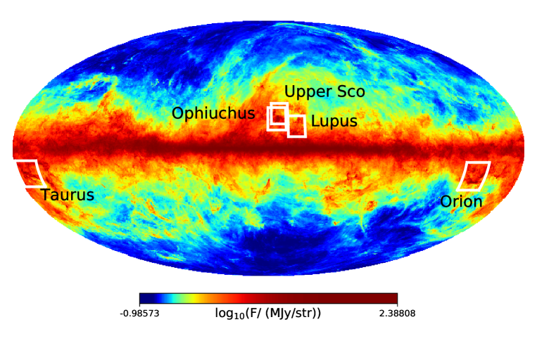
Figure 1: Map of the five star-forming regions analyzed in this paper overlaid on the thermal dust emission at 353 GHz (Planck Collaboration et al., 2016a).

All the five regions are observed in the radio band, in particular with ALMA, and we also use the data for ONC with HST (Hubble Space Telescope) in the optical band (Bally et al., 2000). In what follows, we compile the values of PA from previous literature, and search for the alignment. Details of the five star-forming regions are described below in subsection 3.1-3.5. Table 2-6 in Appendix B summarize the disk parameters.

Table 1: Summary of star-forming regions along with analyses of alignment.

Field	# Disk	Field Size / Resolution	Wavelength	$p$ (Kuiper’s test)	Mean(PA) $\pm$ $\sigma$(PA)	Ref
Lupus	37	$7^{\circ}$ / $0.3\arcsec$	Radio/ALMA	0.29	31.8∘ $\pm$ 114.4∘ a	1
- Lupus III	16/37	$0.5^{\circ}$ / $0.3\arcsec$	Radio/ALMA	0.037	77.3∘ $\pm$ $69.9^{\circ}$ a	1
- Outside Lupus III cloud	21/37	$7^{\circ}$ / $0.3\arcsec$	Radio/ALMA	0.30	298.6∘ $\pm$ 94.3∘ a	1
Taurus	50	$15^{\circ}$ / 0.4–1$\arcsec$	Radiob	0.69	178.66∘ $\pm$ 57.4∘	2–7
Upper Scorpius	16	$8^{\circ}$ / $0.37\arcsec$	Radio/ALMA	0.16	14.6∘ $\pm$ 39.9∘	8
Ophiuchus	49	$3^{\circ}$ / $0.2\arcsec$	Radio/ALMA	0.68	165.5∘$\pm$ 59.1∘	9,10
- L1688	31/49	$0.5^{\circ}$ / $0.2\arcsec$	Radio/ALMA	0.95	156.4∘$\pm$ 59.4∘	9,10
ONC	31	$6\arcmin$ / $0.1\arcsec$	Optical/HST	0.47	21.3∘ $\pm$ 55.9∘	11

References. — (1) Eisner et al. (2018); (2) Kitamura et al. (2002); (3) Andrews & Williams (2007); (4) Isella et al. (2009); (5) Guilloteau et al. (2011); (6) Long et al. (2018); (7) Long et al. (2019); (8) Barenfeld et al. (2017); (9) Cox et al. (2017); (10) Cieza et al. (2019); (11) Bally et al. (2000).

3.1 Lupus

The Lupus clouds are a young (1-2 Myr) and nearby (150-200 pc) star-forming region (Comerón (2008) and references therein). Using ALMA, Ansdell et al. (2016) conducted a systematic survey for radio emission from 89 disks identified by previous literature (Hughes et al., 1994; Comerón, 2008; Merín et al., 2008; Mortier et al., 2011). Out of the 89 disks, Yen et al. (2018) detected CO line emission from 37 disks by a stacking method, and they were able to determine the disk rotation direction spectroscopically. Such measurements can break the degeneracy of the direction of PA, and they obtained the estimate in the range of $0^{\circ}\leq{\rm PA}<360^{\circ}$. In the current analysis, we adopt PA estimated by Yen et al. (2018) instead of those from continuum images.

There is a significant clustering of stars around the Lupus III region. We notice that there exist some overlapping stars, whose radial positions are not consistent with that of the cloud. We exclude such stars on the basis of the parallaxes from Gaia Data Release 2 (Gaia Collaboration et al., 2018), and identify true members in the Lupus III region three-dimensionally. Once the distance to each star, $d$, is given, its location in the equatorial coordinate system is written as

$$(x,y,z)=(d\cos\alpha\cos\delta,d\sin\alpha\cos\delta,d\sin\delta)$$ (4)

where $\alpha$ and $\delta$ are the right ascension, and the declination of the star. Then, we find that the three-dimensional region of the Lupus III cloud is localized in $-60<x\;({\rm pc})<-56$, $-114<y\;({\rm pc})<-106$ as shown in Figure 2, and the spatial extent of the Lupus III region is roughly 5 pc. In the analysis, we exclude systems without Gaia parallaxes: J16011549-4152351, J16070384-3911113, J160934.2-391513, and J16093928-3904316 that are embedded in dark cloud regions and are difficult to be identified in optical bands. In total, our analysis uses 16 disks in the Lupus III region, and 21 disks outside of it, and the typical errors of their PA are less than 10^∘.

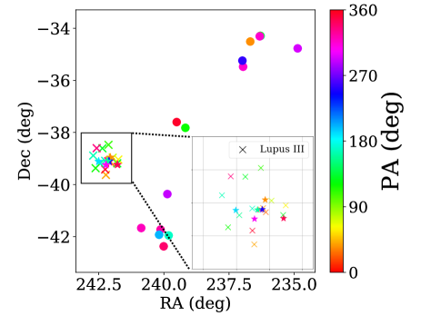
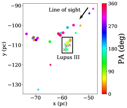
Figure 2: Distribution of disks in the Lupus clouds with measurement of PA in Yen et al. (2018). Left: Locations Positions of disks on the sky plane that are color-coded according to PA. Crosses represent disks in the Lupus III cloud ( $-60<x\;({\rm pc})<-56$, $-114<y\;({\rm pc})<-106$), and star marks indicate the stars, which are unlikely to belong to the region. Right: Disks projected on the x-y plane in the equatorial coordinate system plotted in the same manner as in the left panel. The black arrow indicated the direction of our line-of-sight.

3.2 The Taurus Molecular Cloud

The Taurus Molecular Cloud is a nearby low-mass star-forming region located at 140 pc away. The age for Taurus, especially its disk-hosting population, is typically quoted to be $~{}2$ Myr (e.g. Long et al., 2019). We compile the values of PA published in previous literature (Kitamura et al., 2002; Andrews & Williams, 2007; Isella et al., 2009; Guilloteau et al., 2011; Long et al., 2018, 2019). When more than one estimates are given to the same object, we choose one with the lowest uncertainty. We find that none of the disks in Isella et al. (2009) are chosen based on this criteria. In total, we consider 50 disks in the Taurus region and the errors of their PA values are typically less than $10^{\circ}$.

3.3 The Upper Scorpius OB Association

Upper Scorpius OB Association is a population of stars with the age of 5-11 Myr (Preibisch et al., 2002; Pecaut et al., 2012) located at 145 pc away; Preibisch et al. (2002) and references therein. Unlike the other four regions that we consider in this paper, the molecular gas in the region is already dispersed. Out of 106 possible disk-bearing stars identified by infrared observations (Carpenter et al., 2006; Luhman & Mamajek, 2012), Barenfeld et al. (2016) detected radio emission from 57 systems using ALMA. In the current analysis, we adopt PA estimated by Barenfeld et al. (2017), which presents disk parameters in their Table 1. Unfortunately the majority of disks are not well resolved spatially, and we select 16 stellar systems whose errors of PA are less than $\sim 30^{\circ}$.

3.4 The $\rho$ Ophiuchi cloud complex

The $\rho$ Ophiuchi cloud complex is one of the closest star-forming region located at $\sim 137$ pc away (Ortiz-León et al., 2017), with the stellar age being within 0.5 - 2 Myr (Wilking et al., 2008). In the region, we are particularly interested in the dense cloud L1688 ($246.2^{\circ}<\alpha<247.2^{\circ}$, $-24.8^{\circ}<\delta<-24^{\circ}$) with plenty of resolved disks to look for the possible alignment of their orientations.

This region was surveyed independently by Cox et al. (2017) and Cieza et al. (2019), which we combine in the analysis; Cox et al. (2017) conducted a survey for radio emission from 49 stellar systems with infrared excesses identified by Evans et al. (2003), and found 46 resolved disks using ALMA. The angular resolution of the survey is about $0.2\arcsec$, roughly corresponding to 30 au. We adopt the values of PA listed in their Table 4. More recently, Cieza et al. (2019) obtained continuum images of 147 systems identified by Evans et al. (2009) at $0.2\arcsec$ resolution. Among the 147 observed systems, they were able to spatially resolve 59 disks.

We compile the PA of all the disks identified by the two surveys. Since the PA for face-on disks is difficult to measure reliably, we exclude face-one disks whose inclination angle is consistent with $i=0^{\circ}$ within the $1\sigma$ uncertainty, as well as those disks with PA errors exceeding $30^{\circ}$ as we mentioned before. The combined lists include 51 disks in total, and 17 disks out of them have measured PAs both by the two studies. The mean and standard deviation of their difference, $\Delta$PA, are $-2.3^{\circ}$ and $24.0^{\circ}$, respectively, implying no significant bias between the two measurements. There are two disks with large difference $|\Delta$PA$|\simeq 50^{\circ}$ between the two observations, so we also exclude them from this analysis. For the robust analysis, we try two different combinations in the analysis; one uses Cox et al. (2017) and the other uses Cieza et al. (2019) for the overlapped disks. Finally, our sample contains 49 disks in the entire field of the $\rho$ Ophiuchi cloud complex, out of which 31 systems are located in the cloud L1688.

3.5 Orion Nebula Cluster

The Orion Nebula Cluster (ONC) is one of the closest young stellar clusters embedded in the Orion Nebula. The parent cloud of the Orion Nebula, Orion A, is approximately one order of magnitude larger than ONC in size. ONC is located at $\sim 400$ pc away, and the age is estimated as 2 Myr (Reggiani et al., 2011).

Our analysis of the ONC is based on the optical survey by Bally et al. (2000) that detected 31 disks seen in silhouette in the ONC from the narrow-band images of the Orion Nebula with WFPC2 (Wide Field and Planetary Camera 2) on HST. We use the values of PA listed in their Tables 1 and 2.

The disks in ONC were also observed with ALMA by Eisner et al. (2018), but they did not publish the values of disk PAs. Therefore, we tried to estimate them by ourselves. However, most of the disks look like a point source and are not well resolved even with ALMA. Furthermore, the shapes of point sources in the field turned to be systematically elongated toward the same direction, which is inconsistent with that of the synthesized beam. A similar elongation is also visible in the image of a non-science target in the data set. Thus we suspect that the elongation is not real, and caused by some systematic noise. Indeed, our preliminary analysis suggested an artificial alignment of the disks even at a 6$\sigma$ level. This is why we decided to use the HST data in Bally et al. (2000) for the ONC, instead of the ALMA data in the rest of the paper.

4 Search for non-uniformity of PA in five star-forming regions

We search for the statistical signature of the alignment of PA in the five star-forming regions; Lupus, Taurus, Upper Sco, Ophiuchus, and Orion. Basically, the disks axes are randomly oriented in each region according to the Kuiper test. On the other hand, the Lupus III cloud may exhibit a possible non-unifomity of disk orientations although the statistical significance is barely $2\sigma$ from the analysis of PA alone. Table 3 lists the mean and the standard deviation of PA of disks and the $p$-value from the Kuiper test, which measures the extent to which the cumulative distribution $N(<{\rm PA})$ is consistent with the uniform distribution, for the five star-forming regions. We discuss the results for each region below in order.

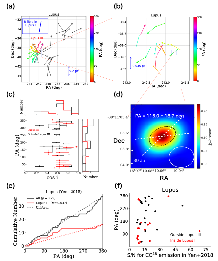
Figure 3: Distribution of disk orientations in the Lupus cloud based on the data published in Yen et al. (2018). (a) Projected disk orientations in the entire field. Arrows represent the direction of the disk position angle (PA), the angle of the major axis of the projected disk ellipse measured counter-clockwise from the north. Due to the spectroscopic data of the Lupus clouds, PA is defined over $0^{\circ}$ and $360^{\circ}$. The small blue square indicates the region of the Lupus III cloud with 16 disks, whose PA directions are color-coded according to the right color-bar. The direction of the magnetic field in the Lupus III region is plotted in the blue arrow inside the top-left box. (b) Zoom-up view of the axis orientations of the 16 disks with spectroscopic measurements of PA in the Lupus III cloud. c) Joint distribution of PA and $\cos$ $i$ of 37 disks measured by Yen et al. (2018); red and black data points correspond to disks inside and outside of the Lupus III region, respectively. (d) Example of a disk image around Sz 90 produced by CLEAN, color-coded according to the surface brightness. The lower-right white ellipse indicates the beam shape, and the black-dotted ellipse represents the disk image deconvolved from the beam. (e) Cumulative distribution of PAs in the entire field (black) and the Lupus III (red). (f) Correlation plot between the signal-to-noise ratio of CO emissions and PA in Yen et al. (2018).

Firstly, we consider the Lupus region. The orientations of 37 disks are summarized in Figure 3, and their distribution projected along the $z$-axis defined in the equatorial coordinate system is plotted in Figure 2. Note that stars in the Lupus III are concentrated in the black box region with the depth of $\simeq 10$ pc. The distribution of PA and $\cos i$ is plotted in Figure 3 (c), and Figure 3 (e) shows the cumulative distribution of PA for the Lupus region. The PA estimated for the Lupus clouds is based on the spectroscopic data of CO lines, allowing the estimate in the range of $0^{\circ}\leq{\rm PA}<360^{\circ}$. Thus, the PA in the Figure 3 (a) is the angle measured counter-clockwise from the north to the direction of each arrow. While the entire Lupus field does not exhibit any preferential direction $(p=0.29)$, the disk axes in the Lupus III cloud are orientated toward the east; Mean(PA) $\pm$ $\sigma$(PA) =$77.3^{\circ}\pm 69.9^{\circ}$. The statistical significance of this non-uniformity is barely $2\sigma$ ($p=0.037$), but the inclination distribution in this region seems to exhibit the consistent correlation as well (Figure 3 (c)). The values of $\cos i$ are clustered around 0.6 for the Lupus III cloud in particular.

Nevertheless this could be an artifact due to the large uncertainties of $\cos i$ in Yen et al. (2018) that might distort the apparent distribution of $\cos i$ around 0.5 when combined with the selection bias toward $\cos i\approx 1$ disks (see Section 2). Therefore, we also examine the distribution of $\cos i$ independently estimated by Ansdell et al. (2016). Indeed their estimates of $\cos i$ for the entire Lupus region do not show a significant peak, but as long as 9 disks with PA in the Lupus III cloud are concerned, the distribution of $\cos i$ by Ansdell et al. (2016) also exhibits a peak around $0.6$. Thus we interpret that the clustering of $\cos i$ for the Lupus III cloud is not an artifact, and consistent with the possible alignment in PA of disks in the region.

We also made sure that the alignment around $77.3^{\circ}$ is not preferentially seen for such disks with lower signal-to-noise ratio. For that purpose, we produce the correlation plot for signal-to-noise ratios of CO emission and PA, both of which are taken from Yen et al. (2018). As the panel (f) of Figure 3 shows, there is no clear correlation between S/N and PA values either in and outside the Lupus III. Thus the possible alignment of the Lupus III cloud is not due to the systematic noise, at least.

In summary, the possible disk alignment in the Lupus III cloud is indicated by both their PA distribution and the clustering of inclination angles around $\cos i=0.6$. Thus the further observation and analysis of the Lupus III cloud is desired to prove or falsify the possible alignment.

The other four regions do not exhibit any significant signature of non-uniformity as shown in Figure 4. Disks in the entire Taurus region are randomly oriented, but those in small sub-regions show a small correlation from the visual inspection, for instance, around $(\alpha,\delta)=(68^{\circ},17.5^{\circ})$, though the statistical discussion is not possible due to limited sample size. In the Upper Scorpius region, the entire field shows weak non-uniformity ($p=0.16$), but it is merely suggestive at best. In the Ophiuchus region, the entire field shows no clear non-uniformity either in the entire region ($p=0.68$) or in the L1688 cloud ($p=0.95)$ if we adopt the values estimated by Cox et al. (2017) for overlapped disks. Although we also attempt the analysis by adopting the estimations from Cieza et al. (2019) for the overlapped systems, we cannot find any signatures of the departure from uniformity either: $p=0.97$ for the entire region, and $p=0.94$ for the L1688 cloud. Finally, 31 disks in the ONC by Bally et al. (2000) do not show any statistically significant signature for the non-uniformity.

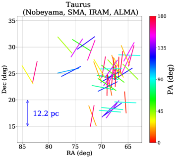
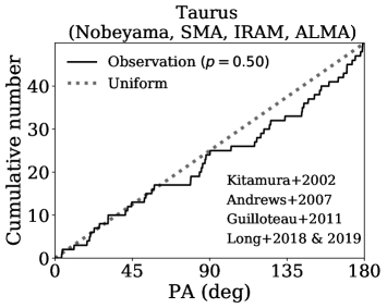
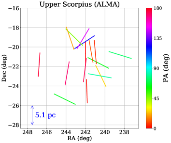
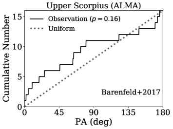
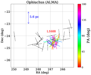
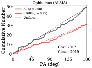
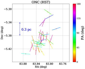
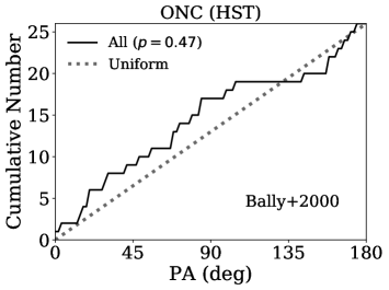
Figure 4: Same as the panels (a) and (e) of Figure 3 for Taurus (Nobeyama, SMA, CARMA, IRAM, and ALMA), Upper Sco (ALMA), Ophiuchus (ALMA), and ONC (HST). Because of the lack of the spectroscopic measurement of PAs, their values can be determined only between $0^{\circ}$ and $180^{\circ}$, thus are represented by bars, instead of arrows.

5 Comparison of different estimators of PA: case of the Lupus cloud

As shown in Section 4, we found no significant signature of the disk alignment except the Lupus III cloud. The result for the Lupus III cloud, however, is still marginal. Therefore, we compare the PA of the Lupus III cloud in Yen et al. (2018) against those that we independently derived using the continuum data. In doing so, we examine the robustness of the derived PAs applying three different methods to continuum images for the Lupus region. While we consider the case of the Lupus clouds specifically, the comparison of the measurements of PAs based on different methods is an important cross-check in general.

The first method “CLEAN$+$imfit” (subsection 5.1) is an intuitive method, which produces the disk image with CLEAN and deconvolves it with an elliptic Gaussian function. The second one “uvmodelfit” (subsection 5.2) directly fits the Gaussian function or disk models to the visibility on the $uv$ plane, instead of the image plane, which has been adapted in literature (e.g Ansdell et al., 2016; Tazzari et al., 2017). Finally, the third method “sparse modeling” (subsection 5.3) creates a super-resolution image of the disk, and estimates the disk parameter by the Gaussian fit. The sparse modeling is now recognized as one of the most powerful techniques in a broad area of science, and indeed it played a vital role recently in the blackhole shadow imaging (Event Horizon Telescope Collaboration et al., 2019). Incidentally, to our knowledge, the present paper is the first attempt to reconstruct multiple proto-planetary disk images using the sparse modeling.

For the purpose of comparison, we choose visibilities measured by Ansdell et al. (2016) and the disks identified in the paper as a fiducial dataset. Out of their ALMA (the Atacama Large Millimeter/submillimeter Array) survey of proto-planetary disks in the Lupus clouds, we analyze 29 disks with estimated PA (listed in their Table 2). First, we download the raw data from the ALMA Science Archive (https://almascience.nao.ac.jp/aq/). Then, we calibrate and reduce the data using CASA 4.4.0. Then, we exclude line emissions and average over the wavelengths using the standard pipelines, and extract the disk continuum emission alone. After the standard calibration, we apply self-calibration that adjusts the gains of antennas using the bright emissions of targets so as to increase the S/N.

5.1 CLEAN$+$imfit

CLEAN is an intuitive and widely-used routine to visualize astronomical objects from the interferometric data. The CLEAN routine first Fourier transforms the observed visibilities, and produces an initial image. Next, it identifies the highest peak beyond the threshold (= 0.001 Jy/Beam in case of the Lupus region in our calculation), which roughly corresponds to 3$\sigma$ level in the image, and subtracts the point spread function (called dirty beam in radio astronomy) at the peak position from the image. The fraction of the subtraction is specified by the gain parameter gain (we adopt gain=0.02 in the current analysis). This process is repeated iteratively, until the maximum flux in the residual image becomes less than the threshold, or the number of iterations exceeds 10,000. Following the procedure in the pipeline, we adopt a Briggs weighting with a robust weighting parameter of 0.5. Here, the Briggs weighting is a combination of natural weighting (constant weights to all visibilities) and uniform weighting (weights inversely proportional to visibility density), and the robust weighting parameter determines the relative ratio of the two weighting (Briggs, 1995). The typical frequency of the observation is $\sim 335$ GHz, and the typical beam size is $0.34^{\prime\prime}\times 0.28^{\prime\prime}$ ($\simeq$ 48 au $\times$ 39 au for 140 pc), which is comparable to the diffraction limit of $\lambda/D_{\rm max}$, with $\lambda$ and $D_{\rm max}$ being the observed wavelength and the maximum length of the baseline. After creating images using the CASA task clean, we deconvolve them with the two-dimensional elliptical Gaussian function using the CASA task imfit, which returns the value of PA and the associated error. Figure 5 shows an example of the disk, Sz 90, in the Lupus clouds imaged by clean.

5.2 uvmodelfit

Instead of measuring the PA of the reconstructed image in real space from interferometric data, one can derive PA directly by analyzing the visibility data on $uv$ plane (e.g Ansdell et al., 2016). In particular, since Fourier transform of the Gaussian function is also Gaussian, the Gaussian fitting can be more directly implemented in the visibility defined on $uv$ plane. Indeed there exists a CASA task uvmodelfit for that purpose, which has been applied to determine PA of disk systems, independently of that based on CLEAN$+$imfit. The non-linear fitting routine implemented in uvmodelfit requires an iteration, which we attempt up to 20 times. Figure 6 shows an example of the analysis with uvmodelfit.

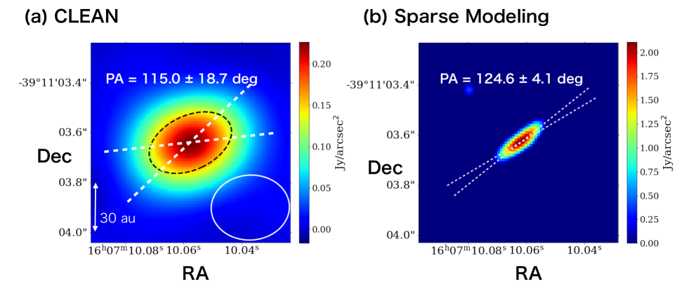
Figure 5: Flux maps of a disk around Sz 90 in the Lupus clouds. The size of boxes is 0.8″$\times$ 0.8″, and we adopt $(\alpha,\delta)$ in J2000. Left: Same as Figure 3 (d). Right: Image created by sparse modeling with $(\Lambda_{l},\Lambda_{t})$ = $(10^{2},10^{2})$. See Section 5.3 and Appendix A for details of the sparse modeling.

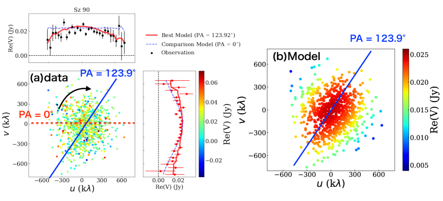
Figure 6: Example of the PA fit for Sz 90 from uvmodelfit in Section 5.2. The points on the $uv$ plane indicate the real part of the visibilities color-coded according to the right-bar. Left: Observed visibilities. Upper and right panels show their projected binned values along $v$ and $u$ directions, respectively. Blue lines show the best-fit model with PA=$123.9^{\circ}$, which should be compared with PA=$115.0^{\circ}\pm 18.7^{\circ}$ (CLEAN) and $124.6^{\circ}\pm 4.1^{\circ}$ (sparse modeling) presented in Figure 5. Lines in the scatter plot show major axes of Gaussian functions on visibility plane. For comparison, we also plot the case of PA $=0^{\circ}$ in red dashed lines. Right: Visibility plots for the best-fit model.

5.3 Sparse modeling

Recent progress in data science indicates a possibility to reconstruct the image of astronomical objects with its angular resolution better than the conventional diffraction limit $\lambda/D_{\rm max}$. In particular, a super-resolution technique on the basis of sparse modeling attracts significant attention, and has proved to be successful in a variety of areas. In short, sparse modeling is one of the mathematical frameworks to estimate the essential information content buried in the data that are dominated by a small number of base functions. In that case, even if the observation samples only a fraction of the entire data space, one may recover the precise information using the sparsity in the solution. Indeed this is very well suited for the radio interferometric observation in which the available $uv$-plane coverage is very limited (e.g. Wiaux et al., 2009; Wenger et al., 2010; Li et al., 2011; Honma et al., 2014; Ikeda et al., 2016; Akiyama et al., 2017a, b; Kuramochi et al., 2018; Event Horizon Telescope Collaboration et al., 2019; Yamaguchi et al., 2020).

Indeed, an effective angular resolution of interferometric images reconstructed with sparse modeling has been shown to become better than 0.2$\sim$0.3 $\lambda/D_{\rm max}$ (e.g. Kuramochi et al., 2018). Thus one can expect that the PA estimated with sparse modeling improves these estimates based on conventional methods including CLEAN$+$imfit and uvmodelfit. Note, however, that our main purpose here is not to identify the small-scale structures of scales $\ll\lambda/D_{\rm max}$, but to estimate PA of the resolved disks after smoothing over their typical sizes $\sim\lambda/D_{\rm max}$. Therefore we do not expect that the PA estimated with sparse modeling is much different from that with CLEAN$+$imfit or uvmodelfit, but do want to make sure of the robustness of the estimated values through their mutual comparison.

We briefly summarize our specific implementation of sparse modeling here, and further details are described in Appendix A.

We would like to find the optimal image data defined on the two-dimensional sky plane, $\bm{I}=\{I_{i,j}\}$, by minimizing the total sum of the difference between the observed visibility $\bm{V}$ and the Fourier-Transform of $\bm{I}$, $\bm{FI}$, and two additional regularization terms:

$$\bm{I}=\mathop{\rm argmin}\limits_{\it I}\left\{\sum_{k}\frac{1}{\sigma_{k}^{2}}(\bm{V}_{k}-(\bm{F}\bm{I})_{k})^{2}+\Lambda_{l}||\bm{I}||_{1}+\Lambda_{t}||\bm{I}||_{\rm tsv}\right\},$$ (5)

where $\bm{V}_{k}$ is the $k$-th observed visibility, $\sigma_{k}$ is the observational error of $\bm{V}_{k}$, and $(\bm{F}\bm{I})_{k}$ is the model visibility corresponding to $\bm{V}_{k}$. In the above, we adopt $l_{1}$ norm of the image and the Total Square Variation (TSV) term as the regularization terms, following Kuramochi et al. (2018). The parameters $\Lambda_{l}$ and $\Lambda_{t}$ control the degrees of sparsity and smoothness of the final image (the detailed explanation is shown in Kuramochi et al. (2018)). The first term is the traditional $\chi^{2}$ term describing the deviations between the model and the data normalized with the errors. The units of $\Lambda_{l}$ and $\Lambda_{t}$ are Jy^-1 and Jy^-2, respectively.

The image $\bm{I}=\{I_{i,j}\}$ is created on 200 $\times$ 200 pixels with one pixel size being $0.1\arcsec$. We use the cross-validation method and find the optimal solution from 20 different sets of $(\Lambda_{l},\Lambda_{t})$: $\Lambda_{l}=10^{0},10^{1},10^{2},10^{3}$ Jy^-1 and $\Lambda_{t}=10^{0},10^{2},10^{4},10^{6},10^{8}$ Jy^-2. Finally, we estimate PA of the resulting images using two methods: fitting with Gaussian function and estimation with tensor of second-order moments $\bm{Q}$ as in Appendix A.2. As for the implementation of sparse modeling, we use Python Module for Radio Interferometry Imaging with Sparse Modeling (PRIISM, Nakazato et al. (2019)). PRIISM solves Eq (5) for a given set of $(\Lambda_{l},\Lambda_{t})$ using the cross validation technique. Panel (b) of Figure 5 shows an image of Sz 90 from sparse modeling with $(\Lambda_{l},\Lambda_{t})$ = $(10^{2},10^{2})$. The image produced by sparse modeling is well resolved compared with that produced by clean.

5.4 Comparison of PA of disks in the Lupus clouds derived from the three methods and previous literature

Now let us compare the values of PA of disks in the Lupus clouds estimated from the three different methods, as well as the published values of PA (Tazzari et al., 2017; Yen et al., 2018). Here, Tazzari et al. (2017) derived geometric parameters for 22 disks by fitting a two-layer disk model to the visibility data from Ansdell et al. (2016). For a fair comparison, we also adopt the completely independent observation in Band 6 (Ansdell et al., 2018), which observed the disks in Ansdell et al. (2016) as well. Although the signal-to-noise ratios in Ansdell et al. (2018) are relatively small, the angular resolution is better ($\sim 0.25\arcsec$) than Ansdell et al. (2016). As there are no published PA in the data presented by Ansdell et al. (2018), we reduce and calibrate the data by ourselves using the prepared pipeline, and derive PA using CLEAN$+{\tt imfit}$.

Therefore, there are seven independent measurements of PA: CLEAN$+{\tt imfit}$, ${\tt uvmodelfit}$, sparse modeling with two estimators of PA, fitting visibility with physical disk model (Tazzari et al., 2017), spectroscopic estimation based on Keplerian motion (Yen et al., 2018), and CLEAN$+{\tt imfit}$ for the data in Ansdell et al. (2018). We adopt the values of PA derived from CLEAN$+$imfit in Ansdell et al. (2016) as the reference of the comparison. Six panels in Figure 7 show the difference $\Delta$PA against reference value (CLEAN$+$imfit with Ansdell et al. (2016)).

Panels (a)-(c) represent the result for the elliptical Gaussian fit of the sparse modeling image, surface brightness tensor of the sparse modeling image, and uvmodelfit, respectively. It is reassuring that the tensor and Gaussian fit of the same image in panels (a) and (b) yield almost identical results. As illustrated clearly in Figure 5, sparse modeling identifies small-scale structures that are impossible to see in the conventional CLEAN image, while they have to be interpreted carefully. Such small-scale structures, however, do not affect the PA measurement of the proto-planetary disks that requires the smoothing over the disk size. Therefore, we made sure that the PA measured from the decomposition of the CLEAN image significantly convolved with the similar beam size is in reality consistent with that independently estimated with sparse modeling.

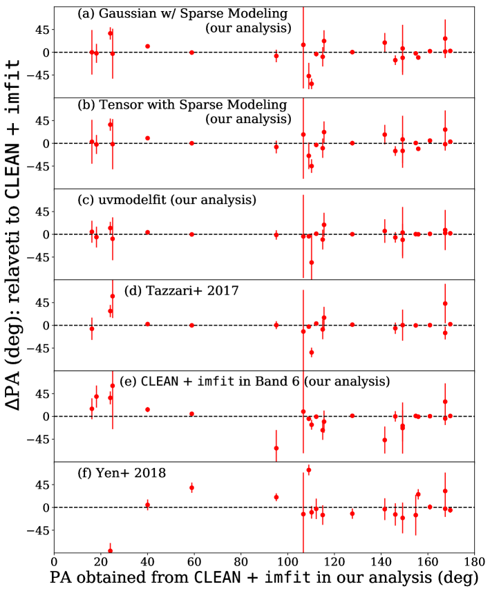
Figure 7: Comparison of PA of disks in the Lupus clouds. Panels (a)-(d) use the same data as in Ansdell et al. (2016). The reference value derived using CLEAN and imfit is plotted in the horizontal axis. The difference of the PA derived from different methods relative to the reference value is plotted in the vertical axis. a) elliptical Gaussian fit of the sparse modeling image, b) tensor fit of the sparse modeling image, c) uvmodelfit, d) Tazzari et al. (2017), e) CLEAN$+$imfit for data in Band 6 (Ansdell et al., 2018), f) Yen et al. (2018).

Panels (a)-(c) present the results for the same dataset (Ansdell et al., 2016) but based on different analysis methods performed by ourselves. In contrast, panel d) presents comparison between our result and Tazzari et al. (2017) that directly fit the visibility data to physical model for the same data, which indicates that both are basically consistent.

Panel (e) plots the comparison of the different datasets (Band 6 of Ansdell et al. (2018), and Ansdell et al. (2016)) but analyzed using the same method (CLEAN + imfit) by us. Again, both datasets yield mostly consistent values, supporting the robustness of the PA values estimated from with the data presented by Ansdell et al. (2016).

Finally, panel (f) shows the comparison with the spectroscopic analysis by Yen et al. (2018), which is also used in the current analysis in Section 4. Out of the 22 overlapped disks, we find that 15 disks satisfy $|\Delta$PA$|$ $<30^{\circ}$, and the mean and the standard deviation of $\Delta$PA are $0.17^{\circ}$ and $30.9^{\circ}$, respectively, implying that the bias is not large, despite the large scatter.

In summary, our systematic comparison using the data for the Lupus region made sure that there is no significant bias in the estimated PA among different analysis methods and datasets, although there are relatively large scatters.

6 Discussion

One of the possible origins of the angular momentum of disks is the random turbulence field in the progenitor molecular cloud cores (e.g. Burkert & Bodenheimer, 2000; Takaishi et al., 2020). If so, one may expect different cloud cores, and thus those disks formed out of them, exhibit no significant alignment of their orientations even if they belong to the same cloud. Our basic finding of the present analysis is, therefore, consistent with the turbulent origin of the angular momentum. On the other hand, the weak signature of the disk alignment of the Lupus III cloud, if real, suggests the presence of additional processes including the coherent global rotation of the initial cloud and/or the magnetic field that account for generation of the angular momentum.

While correlation among the directions of magnetic fields, disk rotations, and jets/outflows have been extensively studied by observations and simulations, there is no consensus yet (Ménard & Duchêne, 2004; Curran & Chrysostomou, 2007; Targon et al., 2011; Hull et al., 2013; Tatematsu et al., 2016; Planck Collaboration et al., 2016b; Mocz et al., 2017; Hull et al., 2017; Stephens et al., 2017; Chen & Ostriker, 2018; Kong et al., 2019). In the following, we present discussion concerning the possible mechanism that generate the disk alignment.

Consider first the magnetic field. The relative importance of the magnetic field may be characterized by the Alfvén Mach number:

$$\mathcal{M}_{\rm A} =\frac{\sigma_{v}}{v_{\rm A}}=\frac{\sqrt{4\pi\rho}}{B}\sigma_{v},$$ (6)

where $\sigma_{v}$ is the turbulent velocity dispersion of the gas, $v_{\rm A}$ is the Alfvén velocity, and $B$ and $\rho$ are the magnetic field and mass density of the gas cloud. It is natural to expect that the magnetic field contributes to the alignment of disk orientations if it exceeds the random turbulent motion of gas, $\mathcal{M}_{A}<1$. Indeed, Planck Collaboration et al. (2016b) found on the basis of the Planck data that all of molecular clouds, including the five regions considered in this paper, are Alfvénic ($\mathcal{M}_{A}\simeq 1$) or sub-Alfvénic $(\mathcal{M}_{A}<1$) by comparing simulations and observations. Furthermore, Hull et al. (2017) found that at least the shape of gas clouds with $\mathcal{M}_{A}<1$ is significantly affected by the magnetic field.

Chandrasekhar & Fermi (1953) derived that the angular dispersion of the magnetic field direction, $\sigma_{\phi}$ (rad), is equal to the Alfvén Mach number. If $\sigma_{\phi}$ is assumed to be the same as $\sigma_{\psi}$ that is the angular dispersion of the polarization vector direction, one can estimate $\mathcal{M}_{\rm A}$ from the observed value of $\sigma_{\psi}$ as

$$\mathcal{M}_{\rm A}\simeq\sigma_{\psi}.$$ (7)

Table D.1 of Planck Collaboration et al. (2016b) shows that $\sigma_{\psi}=36^{\circ}\pm 0.1^{\circ}$ in the Orion region, $\sigma_{\psi}=46^{\circ}\pm 0.1^{\circ}$ in the Lupus cloud, $\sigma_{\psi}=43^{\circ}\pm 0.1^{\circ}$ in the Taurus region, and $\sigma_{\psi}=29^{\circ}\pm 0.1^{\circ}$ in the Ophiuchus region. Therefore, Eq (7) implies that $\mathcal{M}_{\rm A}\simeq 0.6\sim 0.8$, and there is no large difference in values of $\mathcal{M}_{\rm A}$ for those regions. Unless the assumption $\sigma_{\phi}\sim\sigma_{\psi}$ is broken due to the projection effect of polarization vectors, it is unlikely that the strong magnetic field is responsible for the alignment observed only in the Lupus region.

Next, let us consider if the disk orientations in the Lupus III region are somehow related to the global shape and magnetic field of the star-forming regions. For that purpose, we estimate the magnetic field in the region using the Planck polarization map, “COM_CompMap_DustPol-commander_1024_R2.00.fits” at NASA/IPAC Infrared Science Archive, (Planck Collaboration et al., 2016b). The angular resolution is 10$\arcmin$, which roughly corresponds to 1.2 pc in spatial scales for systems at a distance of 400 pc.

The Lupus III cloud exhibits the filamentary structure along the direction PA$\simeq 90^{\circ}$ (Benedettini et al., 2015). There is no associated velocity gradient in the Lupus III cloud, so there is no indication of the rotation (Benedettini et al., 2015). Using the Planck data, we determine the direction of magnetic field to be PA $\simeq 10^{\circ}$ at the scale of 0.3^∘ and $\simeq 170^{\circ}$ the scale of 1^∘ in the Lupus III region adopting the bilinear interpolation. Thus the magnetic field there is also roughly perpendicular to the direction of the filamentary structure (see also Planck Collaboration et al. (2016b)).

Since the spectroscopic data in the Lupus region allow to estimate the PA of the disks in the range of $0^{\circ}\leq{\rm PA}<360^{\circ}$, the derived value of Mean(PA) $\pm$ $\sigma$(PA) =$77.3^{\circ}\pm 69.9^{\circ}$ indicates the coherent rotation of those disks and the disk planes are parallel to the filamentary structure of the gas cloud, and perpendicular to the magnetic field there. It is interesting to note that the directions of filamentary structure and the magnetic field are roughly perpendicular in the Lupus III cloud, and indeed that they are correlated with the disk orientations in the Lupus III cloud. This may be suggestive, but not conclusive at this point. Due to the limited statistics and uncertainties of the disk and magnetic field data, further quantitative analysis is not easy at this point, but additional and future observations would be very rewarding.

Finally we note that the stellar density may be an important parameter for the disk alignment, which varies a lot among the five regions; $4700$ pc^-3 (ONC), $500$ pc^-3 (Lupus III), $6$ pc^-3 (Taurus), $\geq 80$ pc^-3(Upper Sco), and $610$ pc^-3 near L1688 (Ophiuchus) (Nakajima et al., 2000; King et al., 2012). If the mean separations among stars are small, gravitational torques from nearby stars would become significant. In reality, the Lupus III region with the potential alignment has the small scale $\simeq$ 3 pc, in marked contrast to $>10$ pc for Taurus and Upper Sco. On the other hand, since the L1688 or ONC observed by HST does not show any signature of the disk orientation even on a scale of $\sim 1$ pc, the observed size of the region alone does not explain the apparent presence/absence of the disk alignment.

7 Summary and conclusion

The spatial correlation among proto-planetary disk rotations in star-forming regions may carry unique information on physics of the multiple star formation process. In this paper, we focus on five nearby star-forming regions where many proto-planetary disks are spatially resolved with ALMA and HST, and search for the statistical signature of the alignment/non-uniformity of the position angles of the disks.

Our major findings are summarized as follows;

1

We have searched for the spatial correlation of disks among particular five star-forming regions using measured PA. In order to see if the distribution of the PA is consistent to be uniform, we applied the Kuiper test. The PA distribution of the disks in the four regions, Taurus, Upper Scorpius, Ophiuchus, and ONC, is statistically consistent with the random orientation. This result supports the turbulent origin of the disk angular momentum. The 16 disks with with spectroscopic measurement of PA in Yen et al. (2018) in the Lupus III region, a sub-region of the Lupus cloud, show a weak signature of the possible alignment toward the East direction at a $2\sigma$ level. The disk inclination angles also exhibits a concentration, independently supporting the alignment.

2

In order to examine the robustness of the PA in Lupus III, we analysed the continuum images of those disks by ourselves, and compared the result with the measurement by Yen et al. (2018) with those from spectroscopic observations. For that purpose, we applied the three different methods, CLEAN$+$imfit, uvmodelfit, and sparse modeling, for the disk images observed by ALMA in the Lupus region and estimated the PAs by ourselves. We found that our three different sets of PAs are consistent with each other and also with those published in the previous literature. Even though sparse modeling yields a super-resolution image of those disks, the values of PAs are in good agreement with those derived from a conventional method (CLEAN$+$imfit) since the PA represents a global parameter averaged over the size of the disk. Our study confirmed that the measurement of PA is indeed robust in general.

3

In the Lupus III region, the directions of the magnetic field and the filamentary structure are roughly perpendicular, implying that the collapse dynamics of those structures are somehow related to the magnetic field, although not conclusive. Additionally, the disk orientation in Lupus III is fairly aligned with the nearby filament. Since the Planck data imply that the Alfvén Mach number $\mathcal{M}_{\rm A}$ in those five regions is very similar, the magnetic fields equally contribute to kinematics of molecular clouds, and it looks unreasonable to expect the alignment only in the Lupus III region. Therefore the role of the magnetic field in the disk alignment is not clear at this point, but deserves to be revisited with future data.

In addition to the disk alignment that we have studied here, jets and outflows may be used as independent tracers of the stellar spin axes as examined by, e.g., Stephens et al. (2017). While the disk rotation and the stellar spin may be slightly misaligned, such complementary statistics are very important to understand the star formation and evolution of the disk and stellar angular momenta, particularly in the context of the observed spin-orbit misalignment of exo-planetary systems (e.g. Ohta et al., 2005; Bate et al., 2010; Huber et al., 2013; Winn & Fabrycky, 2015; Kamiaka et al., 2018, 2019; Suto et al., 2019). Moreover, investigating the misalignment between stellar and disk axes itself would be interesting (e.g. Davies, 2019).

Our current result is statistically limited, so future analyses or observations of other disk systems are highly desired. The origin of the alignment is still unclear, and magnetohydrodynamical simulations covering the dynamic range from giant molecular cloud down to disk scales (e.g. Kuffmeier et al., 2017; Mocz et al., 2017) or observations (e.g. Hull et al., 2017) are necessary to understand the implication of the statistics of the current result. We have started such attempts by analyzing simulation results using the data given by Chen & Ostriker (2018). Our study is the first step to understand alignment among disks and its implications for star formation, and we hope to report the results of these advanced studies elsewhere.

Appendix A PA measurement of disks using sparse modeling

A.1 Formulation of sparse modeling

In sparse modeling, in addition to the standard chi-squared value $\chi^{2}$, additional regularizations are introduced in the cost function. In this paper, we use the following expression to find the best intensity maps $\bm{I}=\{I_{i,j}\}$ in reference to Kuramochi et al. (2018):

$$\bm{I}=\mathop{\rm argmin}\limits_{\it I}(\chi^{2}(I)+\Lambda_{l}||\bm{I}||_{1}+\Lambda_{t}||\bm{I}||_{\rm tsv})\;\;{\rm s.t.}\;\;{\it I}_{i,j}\geq 0,$$ (A1)

where $||\bm{I}||_{p}$ is the $\Lambda_{p}$ norm of $\bm{I}$:

$$||\bm{I}||_{p}=\left\{\sum_{i}\sum_{j}|I_{i,j}|^{1/p}\right\}^{p}.$$ (A2)

The first term $\chi^{2}(\bm{I})$ in Eq (A1) is the standard $\chi^{2}$-term that expresses the difference between observed and model visibility in the complex plane:

$$\chi^{2}(\bm{I})=\sum_{k}\frac{1}{\sigma_{k}^{2}}(\bm{V}_{k}-(\bm{F}\bm{I})_{k})^{2},$$ (A3)

where $\bm{V}_{k}$ is the $k$-th observed visibility, $\sigma_{k}$ is the observational error associated with $\bm{V}_{k}$, and $(\bm{F}\bm{I})_{k}$ is the model visibility (Fourier transformation of $\bm{I}$) corresponding to $\bm{V}_{k}$. In Eq (A1), $\Lambda_{l}||\bm{I}||_{1}$ is the regularization term with $\Lambda_{1}$ norm, which is known to construct sparse solutions (due to its nature). The coefficient $\Lambda_{\rm l}$ controls sparsity in solutions; the larger $\Lambda_{\rm l}$ prefers sparse solutions (less number of non-zero $I_{i,j}$). Finally, the third term in Eq (A1) is the TSV regularization with the coefficient $\Lambda_{t}$ defined as follows:

$$||\bm{I}||_{\rm tsv}=\sum_{i}\sum_{j}(|I_{i+1,j}-I_{i,j}|^{2}+|I_{i,j+1}-I_{i,j}|^{2}),$$ (A4)

which represents the squared sum of a gradient of an image. By minimizing this TSV regularization, we favor a smooth solution with less variations in $I_{i,j}$. When finding the optimal solution in Eq (A1), we use a monotonic fast iterative shrinkage thresholding algorithm (MFISTA) introduced by Beck & Teboulle (2009a, b) following Akiyama et al. (2017b). We finish fitting until 1000 iterations or achieving convergence; we find that almost all fitting is converged before reaching 1000 iterations. These processes are implemented by PRIISM (Nakazato et al., 2019).

In this paper, we choose $\Lambda_{l}=10^{0},10^{1},10^{2},10^{3}$ (Jy^-1) and $\Lambda_{t}=10^{0},10^{2},10^{4},10^{6},10^{8}$ (Jy^-2) as fiducial coefficients in sparse modeling. The prepared size of $\bm{I}$ is 200 pixels square, where 1 pixel corresponds to $0.01\arcsec$. Among 20 solutions with different sets of $(\Lambda_{l},\Lambda_{t})$, we choose the optimal solutions using 10-fold cross-validation (CV) (see the detail in Akiyama et al. (2017a)). In the process of CV, we first separate the data into training and testing sets. Specifically, we randomly partition the visibility into 10 sets, and we sum up 9 sets as training data, to which we apply the sparse modeling. Then, we compute the Mean Squared Error (MSE) between the testing data and the model visibility obtained from fitting the training data. We iterate this process 10 times by choosing different training sets, and we derive the mean of MSE as well as the standard deviation of mean MSE; the standard deviation of mean MSE is computed as the standard deviation of values of MSE divided by $\sqrt{10-1}$. Finally, we obtain 20 images with MSE and its error {MSE_i, $\sigma({\rm MSE}_{i})$} for sets of $(\Lambda_{l},\Lambda_{s})$. In CV, the lower value of MSE is favored as solutions, so we determine the image with lowest MSE to be the best solution with {MSE_best, $\sigma({\rm MSE}_{\rm best})$}.

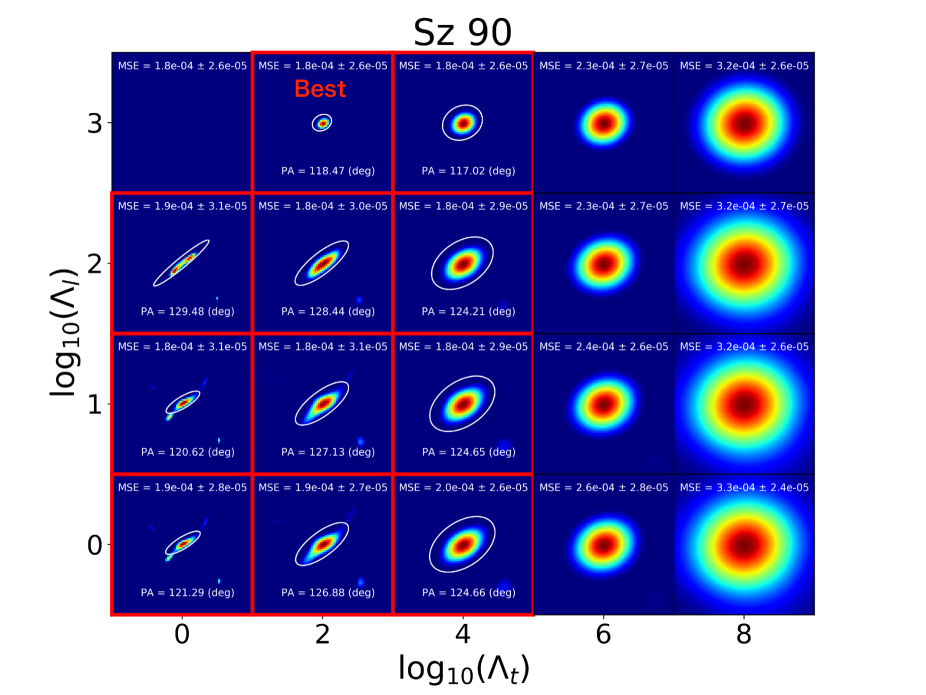
Figure 8: Imaging of a disk around Sz 90 using sparse modeling. The size of each box is 0.8″$\times$ 0.8″. There are 20 images corresponding to combinations of $\Lambda_{1}$ and $\Lambda_{\rm tsv}$. We also show Mean Squared Error (MSE) and its 1$\sigma$ uncertainty in the panels. Red panels have MSE less than ${\rm MSE}_{\rm best}$ + $\sigma({\rm MSE}_{\rm best})$ (consistent with lowest MSE within 1$\sigma$ level). In computing PA, we only use the data in the white ellipse. The average value of PA among likely solutions (red panel) is PA = $124.6\pm 4.1^{\circ}$.

A.2 Methods of estimating PA in sparse modeling

Using the derive images with sparse modeling, we try two methods for estimating PA in this paper. The first method is fitting the two-dimensional elliptical Gaussian function to the images. The second method uses the tensor of second-order brightness moments defined as:

$$\bm{Q}=\frac{\sum_{i}\sum_{j}q(\bm{r}_{i,j},L)I_{i,j}(\bm{r}_{i,j}-\bar{\bm{r}})(\bm{r}_{i,j}-\bar{\bm{r}})^{T}}{\sum_{i}\sum_{j}q(\bm{r}_{i,j},M)I_{i,j}},$$ (A5)

where $\bm{r}_{i,j}=(x_{i},y_{j})$. Here, $q(\bm{r}_{i,j},L)$ is the step function defined as

$$q(\bm{r}_{i,j},L)=\begin{cases}1&(\bm{r}_{i,j}\in M)\\ 0&({\rm otherwise}),\end{cases}$$ (A6)

where the region $L$ determines the non-zero pixels in Eq (A5).

We find that it fails to estimate PA if we use all pixels of the image. This is due to artificial non-zero pixels produced by sparse modeling. Thus, we divide estimations into two steps. As the first step, we roughly determine the region $L$ for the analysis of PA by fitting a Gaussian function to all pixels. Specifically, we determine $L$ to be $3\sigma$ contours of derived Gaussian considering the fact that the signal-to-noise ratios of emissions from disks are $S/N\sim 400$ at most. Then, using the data only in $L$, we derive PA using a Gaussian function and tensor of second-order brightness moments.

Among 20 images with different sets of $(\Lambda_{l},\Lambda_{s})$, we exclude images with large MSE to estimate PA from observations. Specifically, we use PA estimated only from images with MSE less than ${\rm MSE}_{\rm best}$ + $\sigma({\rm MSE}_{\rm best})$. Using the sets of PA, we compute the mean and the standard deviation of them. Figure 8 shows the example of images with sparse modeling, and we find PA = $124.6\pm 4.1^{\circ}$.

Appendix B Tables of disks in five regions

Table 2: Parameters of disks in the Lupus region (Yen et al., 2018).

Name	RA (deg)	Dec (deg)	PA (deg)	$i$ (deg)	$x$ (pc)	$y$ (pc)	$z$ (pc)	In Lupus III?
Sz 65	234.86565	-34.77154	295 ${}^{+20}_{-10}$	$<50$	-73.4	-104.3	-88.6	No
J15450887-3417333	236.28690	-34.29272	170 ${}^{+10}_{-40}$	60 ${}^{+5}_{-15}$	-71.1	-106.5	-87.3	No
Sz 68	236.30354	-34.29194	110 ${}^{+10}_{-5}$	$<45$	-70.7	-106.0	-86.9	No
Sz 69	236.32247	-34.30795	315 ${}^{+10}_{-10}$	$<40$	-70.8	-106.2	-87.1	No
Sz 71	236.68630	-34.51001	35 ${}^{+10}_{-5}$	$<30$	-70.6	-107.4	-88.3	No
Sz 72	236.96088	-35.47660	315 ${}^{+5}_{-5}$	75 ${}^{+5}_{-5}$	-69.2	-106.4	-90.5	No
Sz 73	236.98719	-35.24310	255 ${}^{+5}_{-10}$	$<50$	-69.8	-107.4	-90.5	No
Sz 83	239.17623	-37.82106	120 ${}^{+10}_{-5}$	35 ${}^{+5}_{-15}$	-64.6	-108.2	-97.9	No
Sz 84	239.51043	-37.60086	355 ${}^{+5}_{-5}$	50 ${}^{+5}_{-15}$	-61.4	-104.2	-93.1	No
Sz 129	239.81857	-41.95296	170 ${}^{+40}_{-10}$	70 ${}^{+5}_{-10}$	-60.5	-103.9	-108.1	No
RY Lup	239.86822	-40.36433	290 ${}^{+5}_{-10}$	55 ${}^{+5}_{-5}$	-60.9	-104.8	-103.0	No
J16000236-4222145	240.00976	-42.37082	340 ${}^{+5}_{-5}$	30 ${}^{+5}_{-10}$	-60.6	-105.1	-110.6	No
Sz 130	240.12926	-41.72704	325 ${}^{+10}_{-20}$	55 ${}^{+10}_{-15}$	-59.6	-103.7	-106.7	No
MY Lup	240.18543	-41.92536	200 ${}^{+10}_{-5}$	55 ${}^{+5}_{-5}$	-57.9	-101.1	-104.6	No
Sz 133	240.87239	-41.66727	320 ${}^{+10}_{-5}$	50 ${}^{+5}_{-20}$	-55.7	-99.9	-101.8	No
Sz 88A	241.75244	-39.03885	60 ${}^{+5}_{-10}$	50 ${}^{+5}_{-10}$	-58.2	-108.4	-99.8	Yes
J16070854-3914075	241.78558	-39.23552	345 ${}^{+10}_{-20}$	50 ${}^{+5}_{-20}$	-64.4	-120.0	-111.2	No
Sz 90	241.79190	-39.18435	130 ${}^{+5}_{-5}$	50 ${}^{+5}_{-15}$	-58.8	-109.6	-101.3	Yes
Sz 95	241.96790	-38.96846	75 ${}^{+10}_{-10}$	50 ${}^{+5}_{-15}$	-57.8	-108.6	-99.5	Yes
Sz 96	242.05257	-39.14273	25 ${}^{+5}_{-5}$	$<50$	-56.9	-107.3	-98.8	Yes
J16081497-3857145	242.06234	-38.95412	35 ${}^{+10}_{-5}$	75 ${}^{+5}_{-5}$	-53.1	-100.1	-91.6	No
Sz 98	242.09367	-39.07967	35 ${}^{+10}_{-5}$	50 ${}^{+5}_{-15}$	-56.8	-107.2	-98.5	Yes
Sz 100	242.10729	-39.10044	250 ${}^{+5}_{-20}$	55 ${}^{+5}_{-20}$	-49.7	-93.9	-86.4	No
Sz 103	242.12607	-39.10320	50 ${}^{+5}_{-10}$	50 ${}^{+5}_{-20}$	-57.9	-109.4	-100.6	Yes
J16083070-3828268	242.12786	-38.47423	110 ${}^{+5}_{-5}$	55 ${}^{+5}_{-5}$	-57.1	-108.0	-97.1	Yes
V856 Sco	242.14281	-39.10519	330 ${}^{+10}_{-20}$	40 ${}^{+5}_{-15}$	-58.4	-110.5	-101.6	Yes
Sz 108B	242.17802	-39.10520	160 ${}^{+20}_{-5}$	50 ${}^{+5}_{-20}$	-54.8	-103.9	-95.5	No
J16085373-3914367	242.22384	-39.24365	305 ${}^{+20}_{-5}$	65 ${}^{+5}_{-5}$	-48.3	-91.6	-84.6	No
Sz 111	242.22780	-39.62875	40 ${}^{+5}_{-5}$	$<35$	-56.8	-107.9	-101.0	Yes
J16090141-3925119	242.25584	-39.42008	355 ${}^{+5}_{-5}$	60 ${}^{+5}_{-5}$	-59.1	-112.3	-104.3	Yes
Sz 114	242.25765	-39.08689	170 ${}^{+5}_{-10}$	15 ${}^{+5}_{-5}$	-58.6	-111.5	-102.3	Yes
J16092697-3836269	242.36236	-38.60758	130 ${}^{+20}_{-10}$	65 ${}^{+5}_{-5}$	-57.8	-110.3	-99.4	Yes
Sz 118	242.45268	-39.18811	155 ${}^{+10}_{-5}$	55 ${}^{+5}_{-15}$	-58.8	-112.6	-103.6	Yes
J16100133-3906449	242.50549	-39.11255	190 ${}^{+10}_{-5}$	$<35$	-69.0	-132.5	-121.5	No
J16101984-3836065	242.58259	-38.60194	335 ${}^{+10}_{-5}$	55 ${}^{+5}_{-10}$	-57.1	-110.0	-98.9	Yes
J16102955-3922144	242.62308	-39.37079	120 ${}^{+10}_{-5}$	65 ${}^{+5}_{-10}$	-58.0	-112.1	-103.5	Yes
Sz 123A	242.71489	-38.88726	165 ${}^{+10}_{-20}$	40 ${}^{+5}_{-15}$	-58.1	-112.6	-102.2	Yes

Table 3: Parameters of disks in the Taurus region ((Kitamura et al., 2002; Andrews & Williams, 2007; Guilloteau et al., 2011; Long et al., 2018, 2019))

Name	RA (deg)	Dec (deg)	PA (deg)	cos$i$	$r_{\rm disk}$ (arcsec)a	Refb
04158+2805	64.74287	28.47444	88.0 $\pm$ 5.0	0.60 $\pm$ 0.13	6.20 $\pm$ 0.70	2
AA Tau	68.73093	24.48140	86.0 $\pm$ 5.0	0.46 $\pm$ 0.10	1.34 $\pm$ 0.10	1
BP Tau	64.81598	29.10748	151.1 $\pm$ 1.0	0.79 $\pm$ 0.01	0.23	5
CI Tau	68.46673	22.84169	11.2 $\pm$ 0.1	0.64 $\pm$ 0.00	1.10 $\pm$ 0.00	4
CIDA 9	76.34496	25.52526	102.7 $\pm$ 0.3	0.70 $\pm$ 0.00	0.35 $\pm$ 0.00	4
CQ Tau	83.99361	24.74836	31.0 $\pm$ 8.0	0.73 $\pm$ 0.06	0.86 $\pm$ 0.04	3
CY Tau	64.39053	28.34634	165.0 $\pm$ 4.0	0.85 $\pm$ 0.02	0.55 $\pm$ 0.01	3
DG Tau	66.76955	26.10446	179.0 $\pm$ 3.0	0.82 $\pm$ 0.02	0.56 $\pm$ 0.01	3
DG Tau b	66.76955	26.10446	26.0 $\pm$ 2.0	0.49 $\pm$ 0.04	0.69 $\pm$ 0.03	3
DH Tau A	67.42313	26.54948	18.8 $\pm$ 7.2	0.96 $\pm$ 0.01	0.10	5
DK Tau A	67.68435	26.02351	4.4 $\pm$ 9.8	0.98 $\pm$ 0.01	0.09	5
DL Tau	68.41282	25.34392	52.1 $\pm$ 0.1	0.71 $\pm$ 0.00	0.93 $\pm$ 0.00	4
DM Tau	68.45306	18.16944	134.0 $\pm$ 4.0	0.37 $\pm$ 0.07	2.46 $\pm$ 0.18	1
DN Tau	68.86407	24.24970	79.2 $\pm$ 0.4	0.82 $\pm$ 0.00	0.44 $\pm$ 0.00	4
DO Tau	69.61912	26.18041	170.0 $\pm$ 0.9	0.89 $\pm$ 0.00	0.18	5
DQ Tau	71.72107	17.00004	20.3 $\pm$ 4.3	0.96 $\pm$ 0.01	0.12	5
DR Tau	71.77590	16.97856	170.0 $\pm$ 8.0	0.39 $\pm$ 0.09	0.61 $\pm$ 0.05	2
DS Tau	71.95248	29.41977	159.6 $\pm$ 0.1	0.42 $\pm$ 0.00	0.43 $\pm$ 0.00	4
FT Tau	65.91329	24.93729	121.8 $\pm$ 0.3	0.81 $\pm$ 0.00	0.33 $\pm$ 0.00	4
GI Tau	68.39192	24.35474	143.7 $\pm$ 1.8	0.72 $\pm$ 0.01	0.14	5
GK Tau	68.39401	24.35163	119.9 $\pm$ 9.0	0.76 $\pm$ 0.07	0.07	5
GM Aur	73.79576	30.36649	58.0 $\pm$ 4.0	0.64 $\pm$ 0.05	1.25 $\pm$ 0.05	2
GO Tau	70.76282	25.33853	20.9 $\pm$ 0.2	0.59 $\pm$ 0.00	1.00 $\pm$ 0.01	4
HH 30	67.90613	18.20680	125.0 $\pm$ 0.0	0.15 $\pm$ 0.02	1.43 $\pm$ 0.02	3
HK Tau A	67.96072	24.40494	174.9 $\pm$ 0.5	0.55 $\pm$ 0.01	0.16	5
HL Tau	67.91030	18.23280	144.0 $\pm$ 2.0	0.58 $\pm$ 0.04	1.04 $\pm$ 0.03	1
HN Tau A	68.41401	17.86453	85.3 $\pm$ 0.7	0.35 $\pm$ 0.02	0.10	5
HO Tau	68.83421	22.53738	116.3 $\pm$ 1.0	0.57 $\pm$ 0.01	0.18	5
HP Tau	68.96993	22.90643	56.5 $\pm$ 4.5	0.95 $\pm$ 0.01	0.09	5
HQ Tau	68.94722	22.83934	179.1 $\pm$ 3.3	0.59 $\pm$ 0.05	0.13	5
Haro 6-10 N	67.34888	24.55006	53.0 $\pm$ 18.0	0.38 $\pm$ 0.30	0.24 $\pm$ 0.11	3
Haro 6-10 S	67.34888	24.55006	178.0 $\pm$ 8.0	0.30 $\pm$ 0.19	0.37 $\pm$ 0.05	3
Haro 6-13	68.06424	24.48322	154.2 $\pm$ 0.3	0.75 $\pm$ 0.00	0.18	5
Haro 6-33	70.41179	25.94074	31.0 $\pm$ 28.0	0.79 $\pm$ 0.20	0.57 $\pm$ 0.11	3
Haro 6-5B	65.50288	26.44056	155.0 $\pm$ 8.0	0.56 $\pm$ 0.17	3.40 $\pm$ 0.51	1
IP Tau	66.23784	27.19904	173.0 $\pm$ 0.4	0.70 $\pm$ 0.00	0.27 $\pm$ 0.00	4
IQ Tau	67.46482	26.11246	42.4 $\pm$ 0.2	0.47 $\pm$ 0.00	0.73 $\pm$ 0.01	4
LkCa 15	69.82413	22.35094	79.0 $\pm$ 5.0	0.29 $\pm$ 0.18	2.09 $\pm$ 0.18	1
MWC 480	74.69277	29.84361	147.5 $\pm$ 0.1	0.80 $\pm$ 0.00	0.65 $\pm$ 0.00	4
MWC 758	82.61470	25.33252	168.0 $\pm$ 22.0	0.82 $\pm$ 0.12	1.00 $\pm$ 0.09	3
RW Aur A	76.95653	30.40144	41.1 $\pm$ 0.6	0.57 $\pm$ 0.01	0.10	5
RY Tau	65.48922	28.44320	23.1 $\pm$ 0.0	0.42 $\pm$ 0.00	0.47 $\pm$ 0.00	4
T Tau	65.49763	19.53512	4.0 $\pm$ 17.0	0.71 $\pm$ 0.15	0.48 $\pm$ 0.05	3
T Tau N	65.49763	19.53512	87.5 $\pm$ 0.5	0.88 $\pm$ 0.00	0.11	5
UY Aur	72.94746	30.78710	125.7 $\pm$ 10.6	0.92 $\pm$ 0.06	0.03	5
UZ Tau E	68.17926	25.87525	90.4 $\pm$ 0.1	0.56 $\pm$ 0.00	0.62 $\pm$ 0.00	4
UZ Tau W	68.17926	25.87525	145.0 $\pm$ 24.0	0.82 $\pm$ 0.11	0.40 $\pm$ 0.04	3
V409 Tau	64.54493	25.33261	44.8 $\pm$ 0.5	0.35 $\pm$ 0.00	0.24	5
V710 Tau A	67.99083	18.36026	84.3 $\pm$ 0.4	0.66 $\pm$ 0.00	0.24	5
V836 Tau	75.77750	25.38878	117.6 $\pm$ 1.3	0.73 $\pm$ 0.01	0.13	5

• Notes

• Each disk size follows the definition of corresponding paper.

• References that we used for the analysis: 1. Kitamura et al. (2002), 2. Andrews & Williams (2007), 3. Guilloteau et al. (2011), 4. Long et al. (2018), 5. Long et al. (2019)

Table 4: Parameters of disks in the Upper Scorpius (Barenfeld et al., 2017).

Name	RA (deg)	Dec (deg)	PA (deg)	$i$ (deg)	$r_{\rm disk}$ (arcsec)
2MASS J15534211-2049282	238.42546	-20.81745	73${}^{+5}_{-6}$	89${}^{+1}_{-2}$	0.32${}^{+0.15}_{-0.05}$
2MASS J16014086-2258103	240.42025	-22.96695	26${}^{+22}_{-23}$	74${}^{+10}_{-31}$	0.26${}^{+0.06}_{-0.06}$
2MASS J16020757-2257467	240.53154	-22.95130	80${}^{+17}_{-15}$	57${}^{+14}_{-19}$	0.34${}^{+0.06}_{-0.05}$
2MASS J16024152-2138245	240.67300	-21.63401	63${}^{+28}_{-21}$	41${}^{+14}_{-21}$	0.17${}^{+0.02}_{-0.02}$
2MASS J16035767-2031055	240.99029	-20.51682	5${}^{+22}_{-26}$	69${}^{+21}_{-27}$	0.82${}^{+0.63}_{-0.33}$
2MASS J16054540-2023088	241.43917	-20.38358	10${}^{+36}_{-10}$	67${}^{+9}_{-29}$	0.14${}^{+0.04}_{-0.01}$
2MASS J16072625-2432079	241.85938	-24.53355	2${}^{+19}_{-14}$	43${}^{+10}_{-17}$	0.21${}^{+0.01}_{-0.01}$
2MASS J16075796-2040087	241.99150	-20.66691	0${}^{+15}_{-14}$	47${}^{+8}_{-14}$	0.08${}^{+0.01}_{-0.01}$
2MASS J16081566-2222199	242.06525	-22.36722	173${}^{+24}_{-18}$	86${}^{+4}_{-26}$	0.57${}^{+0.42}_{-0.29}$
2MASS J16082324-1930009	242.09683	-19.50003	123${}^{+3}_{-2}$	74${}^{+5}_{-4}$	0.46${}^{+0.04}_{-0.04}$
2MASS J16090075-1908526	242.25313	-19.13479	149${}^{+9}_{-9}$	56${}^{+5}_{-5}$	0.41${}^{+0.04}_{-0.03}$
2MASS J16123916-1859284	243.16317	-18.98412	46${}^{+22}_{-27}$	51${}^{+14}_{-36}$	0.34${}^{+0.06}_{-0.05}$
2MASS J16142029-1906481	243.58454	-19.10134	19${}^{+32}_{-19}$	27${}^{+10}_{-23}$	0.21${}^{+0.01}_{-0.01}$
2MASS J16153456-2242421	243.89400	-22.70117	170${}^{+10}_{-31}$	46${}^{+12}_{-21}$	0.15${}^{+0.01}_{-0.01}$
2MASS J16163345-2521505	244.13938	-25.35140	64${}^{+9}_{-9}$	88${}^{+2}_{-9}$	0.51${}^{+0.18}_{-0.16}$
2MASS J16270942-2148457	246.78925	-21.80127	176${}^{+25}_{-29}$	70${}^{+15}_{-33}$	0.16${}^{+0.07}_{-0.04}$

Table 5: Parameters of disks in the Ophiuchus region (Cox et al. (2017) and Cieza et al. (2019))

Name	RA (deg)	Dec (deg)	PAcox (deg) a	PAcieza (deg) a	cos $i$ b	$r_{\rm disk}$ (arcsec) b	In L1688?
2MASS J16213192-2301403	245.38301	-23.02799	164.0 $\pm$ 6.6	$\cdots$	0.363 $\pm$ 0.168	0.097 $\pm$ 0.007	No
2MASS J16214513-2342316 (ODISEA_C4_003)	245.43801	-23.70894	174.3 $\pm$ 1.0	174.2 $\pm$ 1.0	0.188 $\pm$ 0.024	0.314 $\pm$ 0.016	No
2MASS J16233609-2402209	245.90047	-24.03923	6.7 $\pm$ 6.5	$\cdots$	0.450 $\pm$ 0.107	0.080 $\pm$ 0.007	No
2MASS J16313124-2426281 (ODISEA_C4_126)	247.88019	-24.44123	49.0 $\pm$ 0.2	56.0 $\pm$ 10.0	0.121 $\pm$ 0.005	0.650 $\pm$ 0.015	No
2MASS J16314457-2402129	247.93574	-24.03708	133.8 $\pm$ 8.9	$\cdots$	0.627 $\pm$ 0.133	0.055 $\pm$ 0.004	No
2MASS J16335560-2442049AB	248.48171	-24.70149	77.0 $\pm$ 15.0	$\cdots$	0.688 $\pm$ 0.123	0.335 $\pm$ 0.042	No
DoAr 25 (ODISEA_C4_039)	246.59867	-24.72064	110.0 $\pm$ 1.4	93.7 $\pm$ 0.2	0.455 $\pm$ 0.021	0.535 $\pm$ 0.019	Yes
DoAr 33	246.91252	-23.97199	78.2 $\pm$ 5.6	$\cdots$	0.782 $\pm$ 0.030	0.113 $\pm$ 0.003	No
DoAr 43a	247.87864	-24.41119	38.3 $\pm$ 1.6	$\cdots$	0.412 $\pm$ 0.026	0.134 $\pm$ 0.004	No
EM* SR 13Aab	247.18861	-24.47204	90.0 $\pm$ 27.0	$\cdots$	0.799 $\pm$ 0.113	0.206 $\pm$ 0.020	Yes
GSS 31a (ODISEA_C4_037A)	246.59734	-24.35000	169.0 $\pm$ 5.0	163.0 $\pm$ 18.0	0.600 $\pm$ 0.074	0.050 $\pm$ 0.002	Yes
GSS 31b	246.59763	-24.35049	147.0 $\pm$ 15.0	$\cdots$	0.718 $\pm$ 0.120	0.035 $\pm$ 0.002	Yes
GY 211 (ODISEA_C4_070)	246.78790	-24.56909	33.1 $\pm$ 1.2	36.1 $\pm$ 2.6	0.479 $\pm$ 0.018	0.133 $\pm$ 0.003	Yes
GY 224	246.79653	-24.67975	92.2 $\pm$ 0.8	$\cdots$	0.346 $\pm$ 0.014	0.214 $\pm$ 0.004	Yes
GY 235 (ODISEA_C4_075)	246.80755	-24.72557	177.0 $\pm$ 13.0	28.8 $\pm$ 7.0	0.827 $\pm$ 0.062	0.104 $\pm$ 0.005	Yes
GY 314 (ODISEA_C4_104)	246.91426	-24.65443	138.9 $\pm$ 2.1	103.7 $\pm$ 2.3	0.562 $\pm$ 0.026	0.129 $\pm$ 0.003	Yes
GY 33 (ODISEA_C4_043)	246.61475	-24.69830	160.5 $\pm$ 1.7	158.9 $\pm$ 1.7	0.288 $\pm$ 0.043	0.169 $\pm$ 0.006	Yes
Haro 1-17	248.09137	-24.70422	79.0 $\pm$ 12.0	$\cdots$	0.474 $\pm$ 0.179	0.068 $\pm$ 0.008	No
IRAS 16201-2410	245.78841	-24.28482	81.4 $\pm$ 8.2	$\cdots$	0.621 $\pm$ 0.086	0.228 $\pm$ 0.021	No
IRS 63 (ODISEA_C4_130)	247.89858	-24.02497	150.0 $\pm$ 5.2	147.1 $\pm$ 0.1	0.689 $\pm$ 0.047	0.261 $\pm$ 0.012	No
L1689-IRS 7B	248.08671	-24.50819	156.0 $\pm$ 28.0	$\cdots$	0.600 $\pm$ 0.355	0.055 $\pm$ 0.007	No
LDN 1689 IRS 5Bb	247.96631	-24.93816	117.0 $\pm$ 17.0	$\cdots$	0.364 $\pm$ 0.295	0.065 $\pm$ 0.013	No
SR 20 W (ODISEA_C4_116)	247.09724	-24.37807	65.7 $\pm$ 1.7	56.0 $\pm$ 5.0	0.345 $\pm$ 0.032	0.210 $\pm$ 0.011	Yes
SR 24b (ODISEA_C4_062)	246.74377	-24.76034	22.5 $\pm$ 8.3	47.5 $\pm$ 3.6	0.572 $\pm$ 0.099	0.492 $\pm$ 0.059	Yes
V935 Sco (ODISEA_C4_005)	245.57718	-23.36349	80.5 $\pm$ 4.7	108.7 $\pm$ 0.3	0.581 $\pm$ 0.051	0.107 $\pm$ 0.005	No
WL6	246.84080	-24.49828	16.0 $\pm$ 28.0	$\cdots$	0.679 $\pm$ 0.282	0.053 $\pm$ 0.009	Yes
WSB 38B	246.69345	-24.20012	108.0 $\pm$ 14.0	$\cdots$	0.384 $\pm$ 0.240	0.043 $\pm$ 0.006	Yes
WSB 60 (ODISEA_C4_114)	247.06876	-24.61624	135.0 $\pm$ 27.0	135.5 $\pm$ 5.8	0.924 $\pm$ 0.063	0.277 $\pm$ 0.013	Yes
WSB 63	247.22530	-24.79575	0.1 $\pm$ 1.3	$\cdots$	0.402 $\pm$ 0.024	0.133 $\pm$ 0.003	No
WSB 67 (ODISEA_C4_121)	247.59749	-24.90459	12.8 $\pm$ 8.4	22.3 $\pm$ 13.5	0.640 $\pm$ 0.084	0.087 $\pm$ 0.005	No
WSB 82 (ODISEA_C4_143)	249.93933	-24.03451	171.6 $\pm$ 2.2	172.3 $\pm$ 0.7	0.486 $\pm$ 0.030	0.650 $\pm$ 0.029	No
YLW 52a	246.96582	-24.52946	129.0 $\pm$ 17.0	$\cdots$	0.491 $\pm$ 0.321	0.108 $\pm$ 0.021	Yes
2MASS J16250692-2350502 (ODISEA_C4_017)	246.27878	-23.84745	$\cdots$	173.8 $\pm$ 1.3	0.299 $\pm$ 0.175	0.117 $\pm$ 0.015	No
2MASS J16253673-2415424 (ODISEA_C4_021)	246.40305	-24.26194	$\cdots$	14.2 $\pm$ 0.0	0.269 $\pm$ 0.018	0.087 $\pm$ 0.002	Yes
2MASS J16253812-2422362 (ODISEA_C4_022A)	246.40880	-24.37697	$\cdots$	15.8 $\pm$ 2.4	0.792 $\pm$ 0.019	0.544 $\pm$ 0.009	Yes
2MASS J16254662-2423361 (ODISEA_C4_026)	246.44430	-24.39348	$\cdots$	107.2 $\pm$ 0.4	0.271 $\pm$ 0.010	0.361 $\pm$ 0.005	Yes
2MASS J16261722-2423453 (ODISEA_C4_033)	246.57180	-24.39605	$\cdots$	71.7 $\pm$ 0.4	0.219 $\pm$ 0.022	0.104 $\pm$ 0.001	Yes
ISO-Oph 37 (ODISEA_C4_038)	246.59823	-24.41111	$\cdots$	48.3 $\pm$ 0.9	0.323 $\pm$ 0.002	0.362 $\pm$ 0.001	Yes
(GY92) 30 (ODISEA_C4_042)	246.60614	-24.38385	$\cdots$	160.3 $\pm$ 0.3	0.743 $\pm$ 0.040	0.112 $\pm$ 0.001	Yes
2MASS J16263778-2423007 (ODISEA_C4_046)	246.65744	-24.38365	$\cdots$	100.5 $\pm$ 7.8	0.842 $\pm$ 0.016	0.223 $\pm$ 0.002	Yes
2MASS J16264046-2427144 (ODISEA_C4_047)	246.66862	-24.45416	$\cdots$	155.7 $\pm$ 1.1	0.833 $\pm$ 0.008	0.409 $\pm$ 0.002	Yes
2MASS J16264285-2420299 (ODISEA_C4_050A)	246.67850	-24.34179	$\cdots$	149.8 $\pm$ 9.8	0.501 $\pm$ 0.180	0.058 $\pm$ 0.006	Yes
2MASS J16264502-2423077 (ODISEA_C4_051)	246.68759	-24.38563	$\cdots$	118.9 $\pm$ 4.0	0.623 $\pm$ 0.003	0.419 $\pm$ 0.001	Yes
2MASS J16265197-2430394 (ODISEA_C4_056)	246.71651	-24.51112	$\cdots$	38.0 $\pm$ 1.5	0.341 $\pm$ 0.052	0.379 $\pm$ 0.019	Yes
2MASS J16265677-2413515 (ODISEA_C4_060)	246.73653	-24.23111	$\cdots$	50.8 $\pm$ 0.5	0.444 $\pm$ 0.044	0.124 $\pm$ 0.005	Yes
2MASS J16270524-2436297 (ODISEA_C4_067)	246.77188	-24.60839	$\cdots$	168.4 $\pm$ 0.9	0.332 $\pm$ 0.022	0.204 $\pm$ 0.003	Yes
2MASS J16270677-2438149 (ODISEA_C4_068)	246.77819	-24.63764	$\cdots$	14.2 $\pm$ 0.9	0.253 $\pm$ 0.043	0.117 $\pm$ 0.004	Yes
2MASS J16271838-2439146 (ODISEA_C4_083)	246.82655	-24.65423	$\cdots$	46.5 $\pm$ 0.6	0.100 $\pm$ 0.017	0.260 $\pm$ 0.002	Yes
2MASS J16273982-2443150 (ODISEA_C4_105A)	246.91590	-24.72098	$\cdots$	118.6 $\pm$ 1.6	0.713 $\pm$ 0.026	0.095 $\pm$ 0.002	Yes

• Notes

• PA_cox is posion angle from Cox et al. (2017), and PA_cox is from Cieza et al. (2019).

• Basically, we list values in Cox et al. (2017). If the values in Cox et al. (2017) are not available, we use values in Cieza et al. (2019).

Table 6: Parameters of disks or jets in ONC (Bally et al., 2000).

Name	RA (deg)	Dec (deg)	PA (deg)	cos$i$	$r_{\rm disk}$ (arcsec)
072-135a	83.78004	-5.35958	108.0	$\cdots$	$\cdots$
109-327a	83.79558	-5.39072	160.0	$\cdots$	$\cdots$
114-426	83.79729	-5.40733	29.0	0.26	1.35
117-352a	83.79887	-5.39772	50.0	$\cdots$	$\cdots$
121-1925	83.80042	-5.32361	118.0	0.62	0.40
132-1832	83.80504	-5.30897	55.0	0.20	0.75
141-301a	83.80892	-5.38367	172.0	$\cdots$	$\cdots$
154-240a	83.81408	-5.37781	100.0	$\cdots$	$\cdots$
163-026	83.81788	-5.34053	159.0	0.25	0.40
165-254	83.81892	-5.38161	4.0	0.33	0.15
172-028	83.82175	-5.34114	140.0	0.57	0.35
174-236a	83.82229	-5.37672	57.0	$\cdots$	$\cdots$
176-543a	83.82313	-5.42850	32.0	$\cdots$	$\cdots$
177-341a	83.82363	-5.39469	105.0	$\cdots$	$\cdots$
179-353a	83.82475	-5.39817	145.0	$\cdots$	$\cdots$
181-247a	83.82533	-5.37981	165.0	$\cdots$	$\cdots$
182-332	83.82575	-5.39208	0.0	0.33	0.15
182-413a	83.82587	-5.40372	86.0	$\cdots$	$\cdots$
183-405	83.82637	-5.40136	43.0	0.71	0.35
183-419a	83.82629	-5.40528	70.0	$\cdots$	$\cdots$
191-232	83.82971	-5.37547	168.0	0.33	0.15
203-504a	83.83442	-5.41783	20.0	$\cdots$	$\cdots$
203-506	83.83458	-5.41825	16.0	0.50	0.20
205-421a	83.83550	-5.40583	70.0	$\cdots$	$\cdots$
206-446a	83.83592	-5.41292	80.0	$\cdots$	$\cdots$
218-354	83.84079	-5.39831	72.0	0.43	0.70
218-529	83.84092	-5.42464	176.0	0.50	0.20
239-334	83.84942	-5.39281	17.0	0.40	0.25
244-440a	83.85175	-5.41111	20.0	$\cdots$	$\cdots$
252-457a	83.85492	-5.41596	160.0	$\cdots$	$\cdots$
294-606	83.87242	-5.43508	86.0	0.25	0.50

• Notes

• PA is estimated from orientations of jets.

References

- Akiyama et al. (2017a) Akiyama, K., Kuramochi, K., Ikeda, S., et al. 2017a, ApJ, 838, 1, doi: 10.3847/1538-4357/aa6305
- Akiyama et al. (2017b) Akiyama, K., Ikeda, S., Pleau, M., et al. 2017b, AJ, 153, 159, doi: 10.3847/1538-3881/aa6302
- Andrews & Williams (2007) Andrews, S. M., & Williams, J. P. 2007, ApJ, 659, 705, doi: 10.1086/511741
- Ansdell et al. (2016) Ansdell, M., Williams, J. P., van der Marel, N., et al. 2016, ApJ, 828, 46, doi: 10.3847/0004-637X/828/1/46
- Ansdell et al. (2018) Ansdell, M., Williams, J. P., Trapman, L., et al. 2018, ApJ, 859, 21, doi: 10.3847/1538-4357/aab890
- Astropy Collaboration et al. (2013) Astropy Collaboration, Robitaille, T. P., Tollerud, E. J., et al. 2013, A&A, 558, A33, doi: 10.1051/0004-6361/201322068
- Astropy Collaboration et al. (2018) Astropy Collaboration, Price-Whelan, A. M., Sipőcz, B. M., et al. 2018, AJ, 156, 123, doi: 10.3847/1538-3881/aabc4f
- Bally et al. (2000) Bally, J., O’Dell, C. R., & McCaughrean, M. J. 2000, AJ, 119, 2919, doi: 10.1086/301385
- Barenfeld et al. (2016) Barenfeld, S. A., Carpenter, J. M., Ricci, L., & Isella, A. 2016, ApJ, 827, 142, doi: 10.3847/0004-637X/827/2/142
- Barenfeld et al. (2017) Barenfeld, S. A., Carpenter, J. M., Sargent, A. I., Isella, A., & Ricci, L. 2017, ApJ, 851, 85, doi: 10.3847/1538-4357/aa989d
- Bate et al. (2010) Bate, M. R., Lodato, G., & Pringle, J. E. 2010, MNRAS, 401, 1505, doi: 10.1111/j.1365-2966.2009.15773.x
- Beck & Teboulle (2009a) Beck, A., & Teboulle, M. 2009a, IEEE transactions on image processing, 18, 2419
- Beck & Teboulle (2009b) —. 2009b, SIAM journal on imaging sciences, 2, 183
- Benedettini et al. (2015) Benedettini, M., Schisano, E., Pezzuto, S., et al. 2015, MNRAS, 453, 2036, doi: 10.1093/mnras/stv1750
- Briggs (1995) Briggs, D. S. 1995, PhD thesis, New Mexico Institute of Mining and Technology
- Burkert & Bodenheimer (2000) Burkert, A., & Bodenheimer, P. 2000, ApJ, 543, 822, doi: 10.1086/317122
- Bussmann et al. (2007) Bussmann, R. S., Wong, T. W., Hedden, A. S., Kulesa, C. A., & Walker, C. K. 2007, ApJ, 657, L33, doi: 10.1086/513101
- Carpenter et al. (2006) Carpenter, J. M., Mamajek, E. E., Hillenbrand, L. A., & Meyer, M. R. 2006, ApJ, 651, L49, doi: 10.1086/509121