Supersoft X-Ray Phases of Recurrent Novae as an Indicator of their White Dwarf Masses

Abstract

We have examined the optical/X-ray light curves of seven well-observed recurrent novae, V745 Sco, M31N 2008-12a, LMC N 1968, U Sco, RS Oph, LMC N 2009a, T Pyx, and one recurrent nova candidate LMC N 2012a. Six novae out of the eight show a simple relation that the duration of supersoft X-ray source (SSS) phase is 0.70 times the total duration of the outburst ($=$ X-ray turnoff time), i.e., $t_{\rm SSS}=0.70~{}t_{\rm off}$, the total duration of which ranges from 10 days to 260 days. These six recurrent novae show a broad rectangular X-ray light curve shape, first half a period of which is highly variable in the X-ray count rate. The SSS phase corresponds also to an optical plateau phase that indicates a large accretion disk irradiated by a hydrogen-burning WD. The other two recurrent novae, T Pyx and V745 Sco, show a narrow triangular shape of X-ray light curve without an optical plateau phase. Their relations between $t_{\rm SSS}$ and $t_{\rm off}$ are rather different from the above six recurrent novae. We also present theoretical SSS durations for recurrent novae with various WD masses and stellar metallicities ($Z=$0.004, 0.01, 0.02, and 0.05) and compare with observed durations of these recurrent novae. We show that the SSS duration is a good indicator of the WD mass in the recurrent novae with a broad rectangular X-ray light curve shape.

1 Introduction

Novae occur in a binary of an accreting white dwarf (WD) and a non-degenerate companion. When the accreted H-rich envelope of the WD reaches a critical mass unstable H-burning sets in. The H-rich envelope expands to a giant size and strong wind mass-loss occurs. The winds are accelerated deep inside the photosphere at around the Fe peak of the radiative opacity ($\log~{}T$ (K) $\sim 5.2$). So they are called the optically thick winds. The wind mass loss continues during the expanded stage of the envelope, through the maximum expansion and in the optical decay phase. The winds stop after a large part of the envelope mass is blown in the wind. Then, the photosphere shrinks to a white dwarf size and the nova enters a supersoft X-ray source (SSS) phase. The main emitting wavelength region of a nova shifts from optical to ultra-violet (UV), and finally to supersoft X-ray until hydrogen burning extinguishes.

The evolution timescales of optical and X-ray phases depend on the WD mass and chemical composition of the envelope. Based on the optically thick wind model (Kato & Hachisu, 1994), Hachisu & Kato (2006) showed that the optical/infra-red (IR) light curves of classical novae are well reproduced with free-free emission from the wind, whereas the supersoft X-ray light curves are roughly reproduced with blackbody emission from the photosphere. Hachisu & Kato (2006) also found that all the optical/IR light curves decay as $F_{\nu}\propto t^{-1.75}$ independently of the WD mass and chemical composition. Here, $F_{\nu}$ is the flux at the frequency $\nu$ and $t$ is the time after the outburst. They call these homologous shapes of light curves “the universal decline law.” The universal decline law is well applied to S (smooth) -type light curve shape novae defined by Strope et al. (2010). The other types of nova light curve shapes deviate from the model light curves in some part. Such exceptions of nova light curves include multi-peaks, secondary maximum, oscillations, dust blackout, jitters, plateau, shock contribution, and so on. However, their global trends of decline can be sometimes fitted with the universal decline law. From multiwavelength light curve fittings, they estimated the WD masses for many novae (Hachisu & Kato, 2006, 2007, 2010, 2015, 2016a, 2018a, 2018b, 2019a, 2019b). In general, a nova on a more massive WD evolves faster. Thus, the supersoft X-ray emergence time $t_{\rm on}$ (the end of the wind phase) and the supersoft X-ray turnoff time $t_{\rm off}$ (the end of shell flash) has a positive linear correlation in the $(\log~{}t_{\rm on})$-$(\log~{}t_{\rm off})$ diagram (e.g. Hachisu & Kato (2010)).

A large sample of classical novae appeared in M31 has been presented by Henze et al. (2011) and Henze et al. (2014). They reported statistical relation between various nova properties, such as the X-ray $t_{\rm on}$ and $t_{\rm off}$, X-ray blackbody temperature, and nova speed class. Figure 8(a) of Henze et al. (2014) shows the $t_{\rm on}$ versus $t_{\rm off}$ diagram, in which the distribution of M31 classical novae indicates a positive correlation. They made a power law fit as

$$t_{\rm off}=1.0^{0.9\pm 1}\times t_{\rm on}^{0.8\pm 1}.$$ (1)

This is different from the theoretical relation obtained by Hachisu & Kato (2010), although Hachisu & Kato’s relation is located in the middle of the scattered data of M31 novae. The reason for the difference is not yet clarified.

A recurrent nova is a nova with multiple recorded outbursts. The optical flux of a recurrent nova generally decays very fast followed by a short SSS phase. Hachisu & Kato (2018b) examined light curves of very fast novae and recurrent novae. They showed that the recurrent novae do not always follow the universal decline law of $F_{\nu}\propto t^{-1.75}$, in contrast to classical novae. The authors clarified the reason why the $V$ light curves deviate from the $t^{-1.75}$ law: (1) contamination with radiation from shock between the ejecta and circumstellar material (V407 Cyg, RS Oph, and LMC N 2009a), and (2) a too short duration of the $F_{\nu}\propto t^{-1.75}$ decline phase followed by a much steeper decline phase of $F_{\nu}\propto t^{-3.5}$ (LMC N 2012a). These effects influence individual recurrent novae differently, which results in a different shape of decline from the $t^{-1.75}$ law. Thus, the decline rate of the $V$/IR light curves is not a good indicator of the WD mass in recurrent novae unlike classical novae.

Henze et al. (2015) pointed out a resemblance of light curves of three recurrent novae, M31N 2008-12a, RS Oph, and U Sco: their X-ray light curves overlap well each other in the normalized timescale with $t=0$ at their optical peaks. In other words, the ratio of the X-ray turn-on time and turnoff time, $t_{\rm on}/t_{\rm off}$, is common among the three novae, independently of the different timescales. Bode et al. (2016) also showed a similarity in the X-ray increase/decrease times between LMC 2009a and KT Eri (see their Figure 22).

Such a proportionality suggests that the recurrent novae has a different $t_{\rm on}$-$t_{\rm off}$ relation from classical novae. In the $t_{\rm on}$ - $t_{\rm off}$ diagram the recurrent nova M31N 2008-12a, having very short $t_{\rm on}$ and $t_{\rm off}$, is located at the shortest edge of, but slightly below, this relation (e.g., Figure 6 in Henze et al. (2015)). It is not clear if this excursion represents different physical property of recurrent novae from classical novae.

In the present work, we examine well-observed recurrent novae to see if they have a clear statistical relation similar to, or different from, those of classical novae. We further examine if the $t_{\rm on}$ - $t_{\rm off}$ relation is closely related to the WD mass, then the SSS duration could be an indicator of the WD mass.

This paper is organized as follows. In Section 2, we compare the $V$ and X-ray light curves of eight recurrent novae including a recurrent nova candidate and measure the X-ray turn-on/turnoff times. Then, we derive a scaling law between $t_{\rm on}$ and $t_{\rm off}$. Section 3 presents our theoretical calculation of SSS durations for recurrent novae on various WD masses and chemical compositions. We then compare our calculated SSS durations with those of the recurrent novae to examine if the SSS duration is a good indicator of the WD mass. Discussion and conclusions follow in Sections 4 and 5, respectively.

Figure 1: Comparison of $V$ and X-ray light curves among the three recurrent novae, M31N 2008-12a, U Sco, and RS Oph. (a) Comparison in normalized timescale against the M31N 2008-12a 2014 outburst. (b) RS Oph. (c) U Sco. (d) M31N 2008-12a in the 2014 (red symbols) and 2016 (blue) outburst. The horizontal black line segments indicate the duration of SSS phase, $t_{\rm SSS}$ (long segment) and $t_{\rm SSS}^{*}$ (short segment). The optical plateau phase is depicted by the horizontal orange line segment in panels (b) and (c). The blue horizontal line segment in panel (d) shows the highly variable phase in the 2016 outburst taken from Henze et al. (2015, 2018). See text for details.

2 Scaling law of SSS phases in recurrent novae

Figure 7 of Henze et al. (2015) shows that the optical light curves of three recurrent novae (M31N 2008-12a, RS Oph and U Sco) are very similar in a normalized timescale and the X-ray light curves overlap well each other. This means that the X-ray turn-on time and turnoff time have the same proportionality relation in these recurrent novae. Figure 1(a) shows the X-ray and optical light curves of the same three recurrent novae as in Henze et al. (2015), but for the absolute $V$ magnitude, $M_{V}$, of the optical light curves. Here, $M_{V}$ is obtained with the distance modulus in $V$ band, $\mu_{V}\equiv(m-M)_{V}=$ 24.8 for M31N 2008-12a, 16.3 for U Sco, and 12.8 for RS Oph (Hachisu & Kato, 2018b). The X-ray count rates of U Sco and RS Oph are shifted in the vertical direction to fit with those of M31N 2008-12a. The light curves are squeezed in the time direction by a factor of 0.21 for RS Oph, and 0.48 for U Sco, against that of M31N 2008-12a.

Figure 1(a) shows that the optical light curve of RS Oph decays slightly slower than the other two novae, M31N 2008-12a and U Sco. Unlike many classical novae, recurrent novae do sometimes not follow the universal decline law, $F_{\nu}\propto t^{-1.75}$, as shown in Figure 24 of Hachisu & Kato (2018b) and Figure 124 of Hachisu & Kato (2019b). Hachisu & Kato (2018b) and Hachisu & Kato (2019b) discussed the physical reason of the deviations. RS Oph decays slowly like $F_{\nu}\propto t^{-1.55}$ because the $V$ flux is contaminated with emission from the shock between the ejecta and circumstellar matter (CSM). V407 Cyg shows a decay trend of $F_{\nu}\propto t^{-1.0}$ in the $V$/$I$ light curves because of much stronger shock heating than that of RS Oph. U Sco follows a trend of $F_{\nu}\propto t^{-1.75}$ law in the very early phase but soon transfers to a much steeper decline of $F_{\nu}\propto t^{-3.5}$ when the wind mass-loss rate sharply drops before it enters the plateau phase owing to the disk irradiation. In M31N 2008-12a, the observational data are obtained only in the early phase and show a similar decay to U Sco. In this way, the differences in the optical light curves are already discussed in Hachisu & Kato (2018b) and Hachisu & Kato (2019b), so in the following subsections, we focus on the X-ray light curves, especially their turn-on and turnoff times.

2.1 Definition of $t=0$, $t_{\rm on}$, and $t_{\rm off}$

In the present work we define the origin of time $t=0$ to be the optical peak. The X-ray turn-on time (turnoff time) is the time in units of days from $t=0$ when the X-ray flux rises (decreases) to a tenth of its peak value. Note that these definitions are different from those often used in X-ray observations of novae.

2.2 RS Oph

Figure 1(b) shows the optical and X-ray light curves of RS Oph in the 2006 outburst. The optical data are the same as those in Hachisu et al. (2006b), and the Swift X-ray data are taken from Hachisu et al. (2007). Hachisu et al. (2006b) modeled the optical light curve with a combination of the WD photosphere, accretion disk, and companion star, both irradiated by the H-burning WD. They explained the plateau phase by the bright accretion disk irradiated by the WD, and concluded that the end of the plateau phase corresponds to the end of hydrogen burning.

To compare the SSS duration with other recurrent novae, we define the SSS phase by the count rate larger than one tenth of its peak value. This phase is indicated by the longer black line segment in Figure 1(b). We obtain $t_{\rm on}=30$ day, $t_{\rm off}=88$ day, and the duration of $t_{\rm SSS}\equiv t_{\rm off}-t_{\rm on}=58$ days.

The supersoft X-ray count rate varies two orders of magnitude in the early SSS phase until day $\sim 46$. This extremely variable phase was discussed in detail by Osborne et al. (2011). From the theoretical point of view, the optically thick wind becomes very weak just before its final stop in the early stage of the SSS phase. The envelope becomes optically thin as the mass-loss rate decreases. If the wind acceleration becomes unstable and correspondingly the wind mass-loss rate becomes variable, the supersoft X-ray flux could largely change from time to time. Such a mechanism has not been studied yet, but it could be one of the explanations on a highly variable X-ray phase.

If it is the case, we should allocate the highly variable X-ray phase to still the theoretical wind phase, and regard the end of the variable phase as the X-ray turn-on time. Thus, the X-ray turn-on time becomes longer while the SSS phase becomes shorter. We express them by $t_{\rm on}^{*}$ and $t_{\rm SSS}^{*}$ and distinguish them from $t_{\rm on}$ and $t_{\rm SSS}$ which are defined by the period when the X-ray count rate is larger than one tenth of the maximum value. As shown in Figure 1(b), the extremely variable phase ends on day 46 but, after that, the X-ray flux seems to be still variable with small amplitudes. Thus, we safely assume that the stable X-ray phase starts on day 56. So we have $t_{\rm on}^{*}=56$ day and $t_{\rm off}=88$ day, and $t_{\rm SSS}^{*}=32$ days. This phase is depicted by the shorter black line segment, slightly above the longer black line segment, in Figure 1(b).

2.3 U Sco

Figure 1(c) shows the optical and X-ray (0.3 - 10 keV) light curves of U Sco in the 2010 outburst. The data are the same as those in Hachisu & Kato (2018b). U Sco is a high inclination binary having the orbital period of 1.23 days (Schaefer, 2010). The narrow dips of the optical light curve in Figure 1(c) show eclipses by the companion star. The WD surface is occulted by the elevated disk surface, so we observe X-ray photons, not directly from the WD surface, but scattered by hot plasma around the WD via Thomson scattering (Ness et al., 2012; Orio et al., 2013). Orio et al. (2013) analyzed X-ray spectral lines on day 18 and 23 observed with Chandra and XMM-Newton, respectively, and concluded that mass-loss ceased between day 18 and day 23 because the blue-shifted absorption component, owing to the WD corona, disappeared between them. The X-ray count rate also shows short-time variations which are attributed to the absorption by high-density clumps (Ness et al., 2012; Orio et al., 2013). Orio et al. (2013) concluded that the mass-loss was not a smooth process but accompanied some clumpiness or inhomogeneity in the density around the WD.

Assuming a binary model consisting of an inflated WD, accretion disk irradiated by the hot WD, and lobe-filling companion, Hachisu & Kato (2000a) and Hachisu & Kato (2000b) reproduced the light curve of U Sco 1999 outburst. The optical plateau phase is well explained by a large contribution from the irradiated accretion disk.

We obtain $t_{\rm on}=12$ day, $t_{\rm off}=38$ day, and $t_{\rm SSS}=26$ days for the SSS phase of U Sco as indicated by the long black line segment in Figure 1(c). The X-ray variability seems to be large in the early phase and stabilized later. This variability may be related to partial obscuration by dense blobs falling around the WD or dense clumpy ejecta passing through the line of sight as discussed by Ness et al. (2012) and Orio et al. (2013). If we exclude this variable X-ray phase, we have $t_{\rm on}^{*}=25$ day, $t_{\rm off}=38$ day, and $t_{\rm SSS}^{*}=13$ days.

2.4 M31N 2008-12a

M31N 2008-12a outbursted every year. The optical and X-ray light curves show remarkable resemblance every year except for the 2016 outburst (Darnley et al., 2016; Henze et al., 2018). Figure 1(d) shows the X-ray and $V$ light curves of the 2014 outburst as a representative of the normal outburst. The data are taken from Henze et al. (2015) (X-ray: filled red squares connected by a red line) and Darnley et al. (2015) (optical: red dots). The plateau phase is not clear in this year, but the 2015 data, which are not shown to avoid complication, clearly show the presence of a plateau phase (Darnley et al., 2016). The X-ray variability of the supersoft X-ray phase was studied in detail by Henze et al. (2015) and by Henze et al. (2018); the X-ray count rate shows large-amplitude and short-term variabilities until day 13 (in their definition) after the optical peak, but this variability suddenly disappears after day 13. Such a behavior has been reported in the all outbursts between 2013 and 2016.

For the 2014 outburst we obtain $t_{\rm on}=5.4$ day, $t_{\rm off}=17.5$ day, and $t_{\rm SSS}=12.1$ days for the full SSS duration of M31N 2008-12a as indicated by the long black line, and $t_{\rm on}^{*}=12.0$ day and $t_{\rm SSS}^{*}=5.5$ days by the short black line in Figure 1(d).

Figure 1(d) also show the 2016 outburst in which the data are taken from Henze et al. (2018). It showed unusual behavior; the optical peak is one magnitude brighter, the X-ray count rate is smaller, and the SSS phase ended earlier. It is difficult to determine the X-ray turn-on time because the X-ray data are not smooth. We adopt $t_{\rm on}=4.75$ day, $t_{\rm off}=13.35$ day, and $t_{\rm SSS}=8.6$ days, assuming the X-ray flux rises just before the first data. However, the X-ray flux could increase earlier, say 0.5 days or so. The X-ray count rate also shows variability but with relatively small amplitudes, thus we do not define $t_{\rm on}^{*}$ and $t_{\rm SSS}^{*}$ for the 2016 outburst.

Henze et al. (2018) presented an idea to explain the shorter SSS phase in the 2016 outburst. If the mass accretion resumes soon after the X-ray turn-on, and the WD accretes matter throughout the SSS phase, the duration of which becomes longer because fresh nuclear fuel is continuously supplied. On the other hand, if the mass-accretion does not restart soon because the accretion disk is blown by the wind, the SSS ends earlier than the continuous accretion case. In the 2016 outburst the brighter optical peak suggests that the outburst is stronger than the other years and, as a result, the accretion disk could be completely destroyed. So the mass supply does not occur soon and the SSS duration is shorter. The unusual 2016 outburst indicates that the WD mass is not the only factor that determines the SSS duration in recurrent novae.

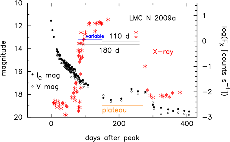
Figure 2: Same as Figure 1, but for LMC N 2009a. The red asterisks indicate the X-ray count rate (0.3 - 10 keV) observed with Swift. The filled black circles and open black circles show $I_{\rm C}$ and $V$ data, respectively, taken from SMARTS (Walter et al., 2012).

2.5 LMC N 2009a

LMC nova 2009a is a recurrent nova with recorded outbursts in 1971 and 2009. Figure 2 shows the X-ray, $V$ and $I$ light curves of LMC N 2009a in the 2009 outburst. The data are the same as those in Figure 33 of Hachisu & Kato (2018b).

Bode et al. (2016) reported the pan-chromatic observations of the 2009 outburst of LMC N 2009a, including UV and X-ray (0.3 - 10 keV) observed by Swift, and $V$ and $I$ magnitudes observed with the Small and Medium Aperture Telescope System (SMARTS) (Walter et al., 2012). This nova is a short orbital period binary and its position in the $(B-R)_{0}$-$M_{B}$ color-magnitude diagram is close to U Sco, which indicates the presence of a bright and hot accretion disk around the WD. Here, $(B-R)_{0}$ is the intrinsic $B-R$ color. The Swift/UVOT-uvw2 light curve shows a plateau phase until $\sim 280$ days after the discovery, indicating a UV-bright disk.

Bode et al. (2016) also reported the strong variability in X-ray. Their Figure 11 shows that the X-ray flux varies largely in the very early SSS phase but becomes static in the later phase. The end of this variable SSS phase is not clear because the Swift observation mode changed from a high to low cadence. We assume that the strongly variable phase ended on day 150 as indicated by the blue line in Figure 2. Thus, we have $t_{\rm on}=80$ day, $t_{\rm off}=260$ day, $t_{\rm SSS}=180$ days, $t_{\rm on}^{*}=150$ day, and $t_{\rm SSS}^{*}=110$ days.

Hachisu & Kato (2018b) analyzed the optical light curve of LMC N 2009a in detail. They pointed out a resemblance of the shape of light curves between RS Oph and LMC N 2009a both for X-ray and $V$, even though the evolution timescale of RS Oph is 3.16 times longer (see their Figure 33). This means that LMC N 2009a also shows the same proportionality relation as that of the three recurrent novae in Figure 1.

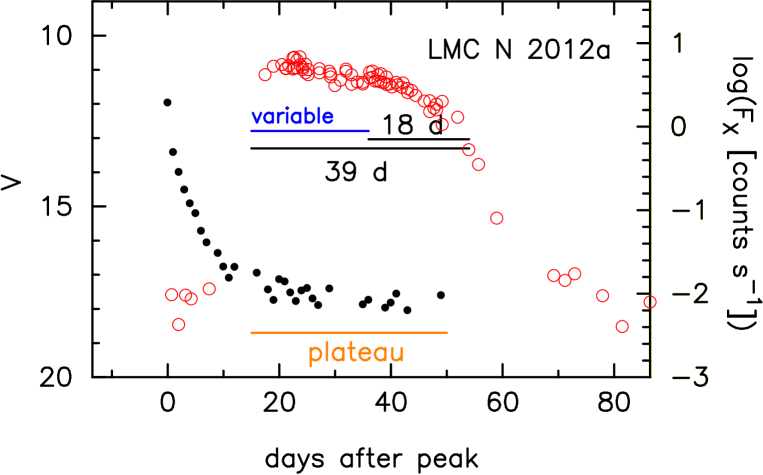
Figure 3: Same as Figure 1, but for LMC N 2012a.

2.6 LMC N 2012a: A recurrent nova candidate

Hachisu & Kato (2018b) pointed out that the $B$, $V$ and $I_{\rm C}$ light curves of LMC N 2012a overlap with those of U Sco including the optical plateau phase (see their Figures 26, 35 and 45). Moreover, the $(B-V)_{0}$ color of LMC N 2012a in the plateau phase agrees well with that of U Sco. Here, $(B-V)_{0}$ is the intrinsic $B-V$ color. Because the optical plateau phase of U Sco is dominated by the irradiated accretion disk, they concluded that LMC N 2012a also has a bright irradiated accretion disk. These resemblance in the light curves and colors as well as a relatively longer orbital period of 0.802 days (Schwarz et al., 2015) strongly suggests that LMC N 2012a is a recurrent nova similar to U Sco. Hachisu & Kato (2018b) estimated the WD mass to be $1.37~{}M_{\odot}$ from a monotonic relation between $M_{\rm WD}$ and time-stretching factor (their Section 5.3).

Figure 3 shows the X-ray and $V$ light curves, the data of which are taken from Hachisu & Kato (2018b). We obtain $t_{\rm on}=15$ day, $t_{\rm off}=54$ day, and $t_{\rm SSS}=39$ days for the full SSS duration of LMC N 2012a.

Schwarz et al. (2015) reported the Swift and Chandra X-ray observations. The X-ray count rate is weakly variable until day $\sim 35$, followed by a smooth decline (see their Figure 14). The hardness ratio defined by ($0.5-10$ keV)$/$($0.3-0.5$ keV) is also variable until day $\sim 37$ (their Figure 4). The exact time of switch from the variable to non-variable phase is not reported, so we define it as $t=36$ day as shown in Figure 3. We have $t_{\rm on}^{*}=36$ day, $t_{\rm off}=54$ day, and $t_{\rm SSS}^{*}=18$ days.

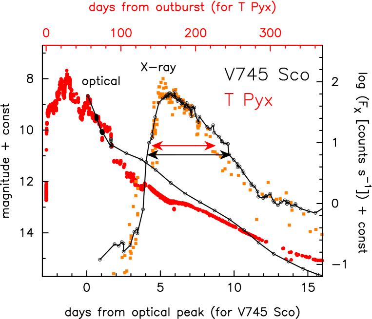
Figure 4: The X-ray and optical light curves of the galactic recurrent novae, V745 Sco in the 2014 outburst (small black open circles connected by a black line: timescale is in the lower axis) and T Pyx in the 2011 outburst (the timescale in the upper side). The optical $V$ light curve of T Pyx is indicated by the red dots. Its magnitude is shifted downward by $1.5$ mag (ranges from $14.2$ mag to $5.2$ mag). The X-ray count rates of T Pyx are indicated by the filled orange squares in the range from $-3.3$ to $0.5$. The X-ray duration is indicated to be $5.7$ days by the two-headed black arrow for V745 Sco, and to be $86$ days by the tow-headed red arrow for T Pyx.

2.7 LMC N 1968

LMC N 1968 outbursted in 1968, 1990, 2002, 2010, 2016, and 2020. Kuin et al. (2020) presented detailed information on multiwavelength light curves of the 2016 outburst including optical and X-ray bands. The optical/IR light curves show a plateau on day 10 - 25 corresponding to the SSS phase. The 2020 outburst data are not published yet, so we use the X-ray light curve in the 2016 outburst.

Figure 8 in Kuin et al. (2020) shows the X-ray count rate of LMC N 1968. There are no data in the middle 10 days. We assume the X-ray light curve has a flat peak and the flux keeps the same value during the missing period. The X-ray turn on/off time is not clear because the flux is not smooth but stays around one tenth of the assumed peak flux. Under the condition we obtain the time since the first discovery (2016 January 21.2094 UT) to be $t_{\rm on}=7.2$ day, $t_{\rm off}=37.4$ day and $t_{\rm SSS}=30.2$ days. There is no information on the presence or non-presence of strong variability.

2.8 V745 Sco

V745 Sco is a symbiotic recurrent nova with recorded outbursts in 1937, 1989, and 2014. The 2014 outburst of V745 Sco evolves extremely fast such that the supersoft X-ray flux increased only four days after the optical discovery. Page et al. (2015) presented the multiwavelength light curves of IR, optical, UV and X-ray bands. From the X-ray spectral analyses, the heavy element abundance of V745 Sco was estimated to be mildly sub-solar, that is, Fe/Fe${}_{\odot}=0.5$ and $0.3-0.7$ by Orio et al. (2015) and Drake et al. (2016), respectively. Figure 4 shows the X-ray light curve obtained with Swift (0.3 - 2 keV: taken from Page et al. (2015)) as well as the $V$ light curve (taken from the American Association of Variable Star Observers (AAVSO) until day 1.65, and SMARTS from day 1.69). The X-ray count rate goes up very quickly to reach the maximum, followed by a slow decay without a plateau phase. No highly variable phase is detected. Page et al. (2015) obtained the X-ray temperature from blackbody fit. Their X-ray temperature increased and then decreased with the X-ray count rate. They interpreted the X-ray decay phase to be the WD cooling phase.

Such a very fast evolution suggests that V745 Sco hosts an extremely massive WD. Hachisu & Kato (2018b) fitted the X-ray light curve of V745 Sco with a theoretical model of 1.385 $M_{\odot}$ WD (see their Figure 7). The envelope mass is very small and a substantial part of the ignition mass is already blown in the wind before the X-ray flux turns on. This small envelope mass results in a quick rise and immediate drop in the X-ray count rate, skipping a plateau phase of X-ray. In this model, the X-ray decay phase corresponds to the WD cooling phase, being consistent with the interpretation by Page et al. (2015).

The X-ray light curve of V745 Sco shows a narrow “triangle” shape, not a broad “rectangle” shape like the other six novae. The X-ray plateau phase, like in RS Oph, corresponds to the steady nuclear-burning phase (Hachisu et al., 2006b), where the envelope mass gradually decreases owing to hydrogen burning. If the envelope mass is very small, the steady burning phase is also short. V745 Sco has neither highly-variable X-ray phase nor flat peak. The envelope mass may be extremely small and mostly blown off before it enters an SSS phase. This is the reason for the narrow triangle shape of X-ray light curve. In the cooling phase of the WD, the X-ray flux drops quickly, so the irradiation effect of the disk is small. Even if V745 Sco has a large disk, we do not expect an optical plateau phase in the cooling phase of the WD. This is the reason why V745 Sco shows no plateau phase in the $V$ light curve.

Although the X-ray light curve shape is different, we adopt the same definition of X-ray turn on/off time, i.e., the epoch of one tenth of the peak X-ray flux as the other recurrent novae. This phase is indicated by the two-headed black arrow in Figure 4. We obtain $t_{\rm on}=4.1$ day, $t_{\rm off}=9.8$ day and $t_{\rm SSS}=5.7$ days.

2.9 T Pyx

T Pyx is a recurrent nova with the recored outbursts in 1890, 1902, 1920, 1944, 1967 and 2011 (Schaefer, 2010; Schaefer et al., 2013). The optical light curve is characterized by a relatively slow evolution and multiple peaks (Nelson et al., 2014; Chomiuk et al., 2014). Its orbital period, 0.076 days (=1.8 hr) (Schaefer et al., 2013), is located below the period gap. The orbital period suggests an exceptionally low-mass companion, although very high mass-accretion rates are usually not expected in such a short orbital period companion. The multiple peak in the optical light curve suggests that a single explosion model may not be applicable. Moreover, as shown later, the X-ray light curve has a narrow triangle shape without a broad flat peak. These properties make T Pyx very different from the other recurrent novae.

The X-ray and optical light curves of the 2011 outburst are shown in Figure 4. The optical $V$ data (red dots) are taken from AAVSO. The X-ray count rates obtained with Swift (filled orange squares) are taken from the Swift website (Evans et al., 2009). The X-ray light curve shows a quick rise followed by a slower decrease. Its shape is a triangle. We obtain $t_{\rm on}=141$ day, $t_{\rm off}=227$ day and $t_{\rm SSS}=86$ days.

Figure 4 compares the light curve of T Pyx with that of V745 Sco. The timescale ratio is 20. Here we fit the optical maximum of V745 Sco with the last optical maximum of T Pyx. Despite of a 20 times slower evolution in T Pyx, both the X-ray light curves show a homologous triangle shape. Because there are no theoretical light curve fitting models for T Pyx, we do not go into detail of the evolution of this atypical recurrent nova.

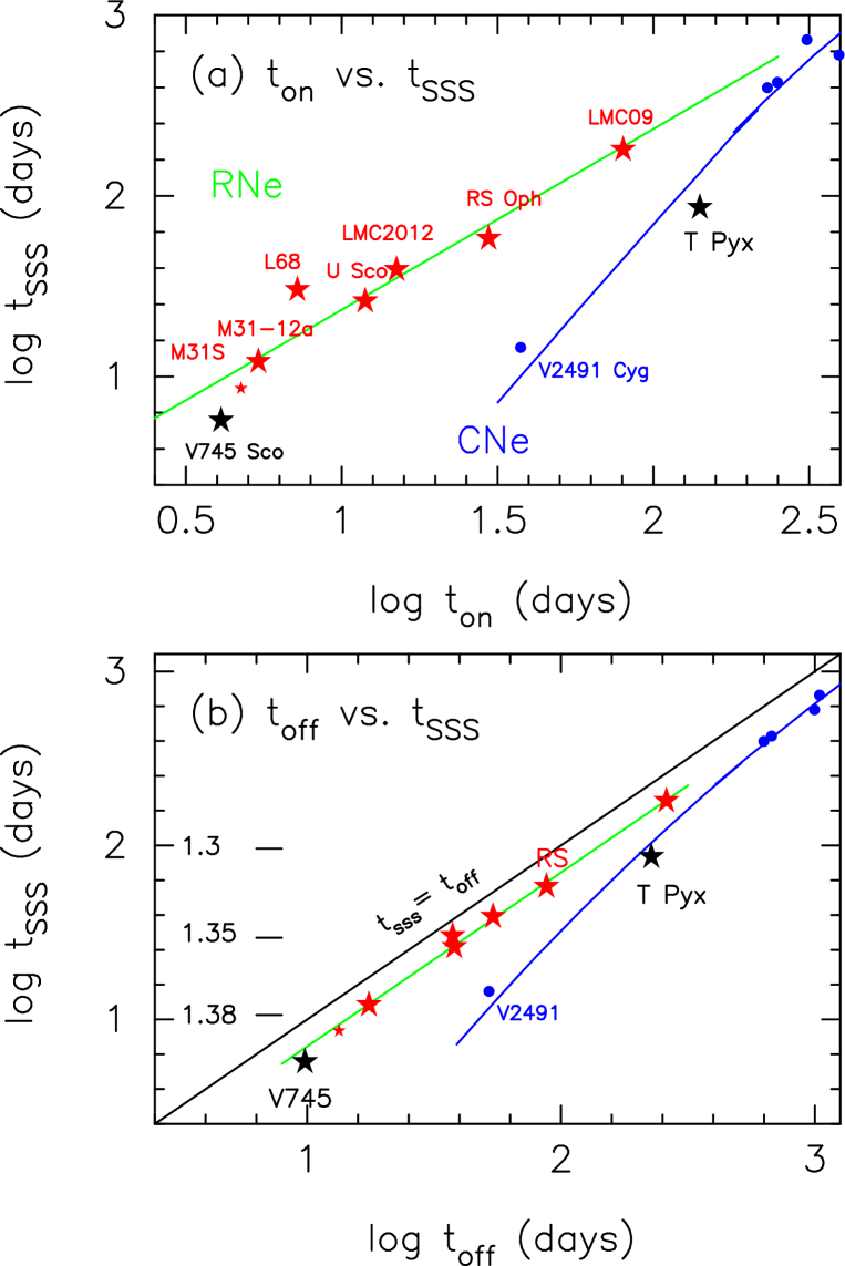
Figure 5: The duration of the SSS phase of various recurrent and classical novae against (a) X-ray turn-on time, and (b) X-ray turnoff time. The red stars indicate, from left to right, M31N 2008-12a (small symbols for the 2016 outburst and large symbols for the 2014 outburst), LMC N 1968, U Sco, LMC N 2012, RS Oph, and LMC N 2009a. The black stars indicate the recurrent novae, V745 Sco (left) and T Pyx (right). The five blue dots represent the position of the classical novae, from lower left to upper right, V2491 Cyg, V1974 Cyg, V1494 Aql, V458 Vul, and V1213 Cen. The blue line shows the theoretically derived relation for classical novae (see Appendix A). The green lines represent the empirical relations, i.e., Equation (2) in panel (a), but Equation (3) in panel (b). The black line in panel (b) indicates the relation, $t_{\rm SSS}=t_{\rm off}$. In panel (b) LMC N 1968 is located very close to, but slightly above, U Sco.

2.10 Scaling Law of Recurrent Novae

In the previous subsections, we have obtained the durations of SSS phases for eight recurrent novae including one candidate. Figure 5 shows $t_{\rm SSS}$ against (a) $t_{\rm on}$ and (b) $t_{\rm off}$ of these eight recurrent novae. The five novae, M31N 2008-12a, U Sco, LMC N 2012a, RS Oph, and LMC N 2009a are located on a straight line. We draw a green straight line of inclination 1.0 to fit these five nova data, which is defined by

$$\log t_{\rm SSS}=\log t_{\rm on}+0.37,$$ (2)

in panel (a) and

$$\log t_{\rm SSS}=\log t_{\rm off}-0.155,$$ (3)

in panel (b). From these two equations, we have the proportionality relations,

$$t_{\rm on}=0.30~{}t_{\rm off},$$ (4)

and

$$t_{\rm SSS}=0.70~{}t_{\rm off}.$$ (5)

LMC N 1968 is located substantially above the green line of Equation (2). We suppose that this deviation comes either from scatter of the X-ray data points around $t_{\rm on}$ and $t_{\rm off}$ or from some physics that keeps the X-ray count rate high at one tenth of the peak level that is not observed in the other recurrent novae. In the 2020 outburst or after, we expect that much more detailed information on the X-ray flux is available.

The two recurrent novae with a triangle shape of X-ray light curve are located much below the green line of Equation (2) in Figure 5(a). The position of T Pyx is rather close to the theoretical line for classical novae (blue). V745 Sco is located near the shortest limit of the curving alignment of recurrent novae that seems to apart downward from the green line in panel (a). Note, however, that $t_{\rm on}$ of M31N 2008-12a in the 2016 outburst (small star) is very uncertain. The position of M31N 2008-12 2016 outburst could be in the middle of M31N 2008-12a 2014 outburst and V745 Sco as in Figure 5(a), but it could move toward upper-left and approach closer to the green line, if we assume a shorter, say 0.5 days shorter $t_{\rm on}$. Thus, it is uncertain whether V745 Sco is the shortest edge of the curving alignment (sudden drop from the green line at M31N 2008-12a) of the recurrent novae, or an exception from the straight line, Equation (2).

To clarify the difference of recurrent novae from classical novae, we plot the theoretical relation derived for the classical nova models (Hachisu & Kato, 2010) (see Appendix A for derivation). We also added five classical novae denoted by the blue dots. They are, from lower-left to upper-right, V2491 Cyg (data taken from Figure 1 in Hachisu & Kato (2009), Page et al. (2010); Ness et al. (2011)), V1974 Cyg (Figure 38 in Hachisu & Kato (2016a)), V1494 Aql (Figure 22 in Hachisu & Kato (2010)), V458 Vul (Figure 67 in Hachisu & Kato (2016c)), and V1213 Cen (Figure 65 in Hachisu & Kato (2019b)). These five novae are located consistently on the blue line. The position of V2491 Cyg demonstrates that classical novae have different physical properties from recurrent novae. These two lines are close in the longer $t_{\rm on}$ (or $t_{\rm off}$), but largely different in the shorter $t_{\rm on}$ (or $t_{\rm off}$). We safely conclude that recurrent novae have a longer SSS phase than classical novae that have the same $t_{\rm on}$ (or $t_{\rm off}$) time.

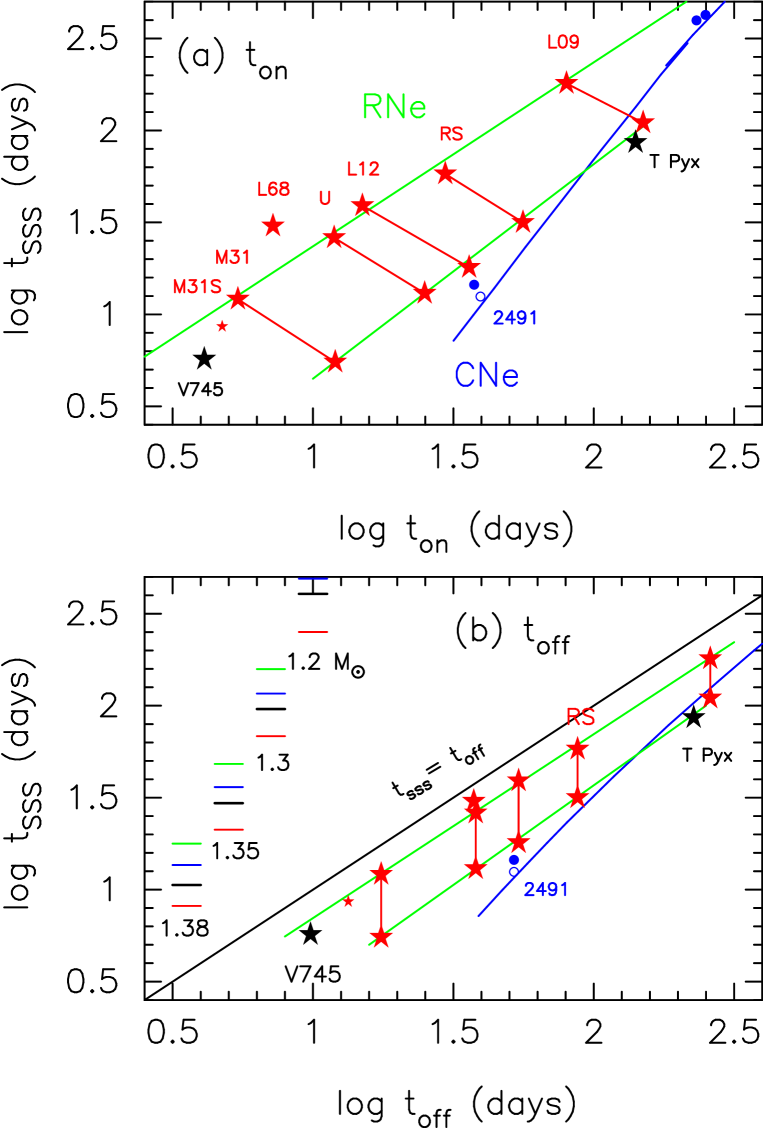
Figure 6: Same as Figure 5, but we added $t_{\rm SSS}^{*}$, the SSS duration excluding the highly variable phase, that are indicated by the lower red stars connected with each $t_{\rm SSS}$ point (above red stars). The lower green straight lines indicate empirical relations, $t_{\rm SSS}^{*}$ vs. $t_{\rm on}^{*}$ of Equation (6) in panel (a), but $t_{\rm SSS}^{*}$ vs. $t_{\rm off}$ of Equation (7) in panel (b). See text for more details.

Figure 6 shows the same $t_{\rm SSS}$ as those in Figure 5, but we added another definition of the SSS phase, which starts after the variable X-ray phase ends, $t_{\rm SSS}^{*}$. The five novae are located along the lower green line, which is defined by

$$\log~{}t_{\rm SSS}^{*}=1.17~{}(\log~{}t_{\rm on}^{*}-1.0)+0.65,$$ (6)

in Figure 6(a) and

$$\log~{}t_{\rm SSS}^{*}=1.08~{}(\log~{}t_{\rm off}-1.2)+0.7,$$ (7)

in Figure 6(b). These lines are calculated from the positions of the five recurrent novae with a broad rectangular SSS phase, and not parallel but slightly steeper than Equations (2) and (3). The two SSS periods, $t_{\rm SSS}$ and $t^{*}_{\rm SSS}$, of each nova are connected by the line. Interestingly, T Pyx is located on the lines of $t_{\rm SSS}^{*}$ in both the upper and lower panels. Its position is also close to the blue classical nova line.

The classical nova V2491 Cyg also shows highly variable SSS phase as reported by Ness et al. (2011). Their Figure 1 demonstrates a deep dip on day $\sim 39$ in the Swift X-ray count rate. If we exclude the part before the dip, we have a two-days shorter period, $t_{\rm SSS}^{*}=12.5$ days compared with $t_{\rm SSS}=14.5$ days (blue open circle in Figure 6). In both the upper and lower panels, $t_{\rm SSS}^{*}$ of V2491 Cyg is more closer to the theoretical line of classical novae (blue line).

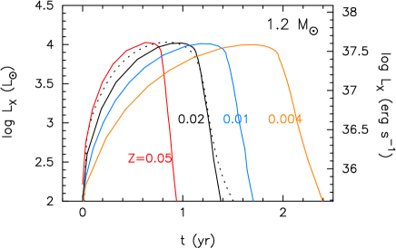
Figure 7: The X-ray ($0.3-1.0$ keV) light curve in the SSS phase of a recurrent nova on a 1.2 $M_{\odot}$ WD with the metallicity of $Z=$0.004 (orange), 0.01 (blue), 0.02 (black), and 0.05 (red). The dotted line indicates the evolution model for a 1.2 $M_{\odot}$ WD with $Z=0.02$ (Kato et al., 2017a).

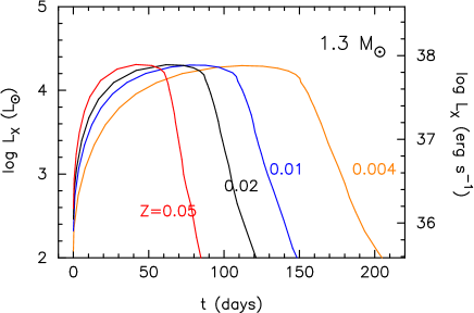
Figure 8: Same as Figure 7, but for a 1.3 $M_{\odot}$ WD.

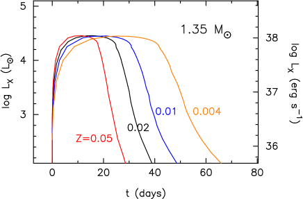
Figure 9: Same as Figure 7, but for a $1.35~{}M_{\odot}$ WD.

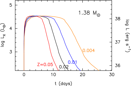
Figure 10: Same as Figure 7, but for a 1.38 $M_{\odot}$ WD.

3 SSS durations of recurrent novae

3.1 Numerical Models

The supersoft X-ray source phase of post nova outburst has been theoretically calculated for various WD masses and chemical compositions of hydrogen-rich envelopes (Kato & Hachisu, 1994; Kato, 1999; Sala & Hernanz, 2005; Wolf et al., 2013; Kato et al., 2013). These calculations, however, did not exactly cover the parameter region for recurrent novae. Thus, we have calculated the SSS phases and X-ray light curves for extended ranges of parameters. The numerical method is the same as that in Kato & Hachisu (1994), in which the optical decay phase is followed by a sequence of optically-thick wind solutions. After the winds stop, an SSS phase is followed by a sequence of hydrostatic solutions.

To calculate the envelope solutions, we need to assume the WD radius and chemical composition of the envelope. These values are taken from our evolution calculations of shell flashes already published. Although the WD accretes solar composition ($X=0.7$, $Y=0.28$, and $Z=0.02$) material, convection widely develops at the outburst and a part of nuclear ash helium of the previous outburst is dredged up and mixed into the whole envelope. As a result, hydrogen mass fraction decreases by some amount from the original $X=0.7$, and helium mass fraction increases by the same amount. This hydrogen decrease is larger in more massive WDs. We adopt WDs of $1.2~{}M_{\odot}$, $1.3~{}M_{\odot}$, $1.35~{}M_{\odot}$, and $1.38~{}M_{\odot}$. The mass accretion rates of our published models do not cover enough fine grid, but the dependence of composition and radius on the mass accretion rate is not large as far as the recurrence period is less than a few tens of years.

The envelope chemical composition and WD radius for the $1.2~{}M_{\odot}$ WD are assumed to be $(X,Y,Z)=(0.6,0.38,0.02)$ and $\log(R_{\rm WD}/R_{\odot})=-2.200$. These values are taken from the time-dependent nova model of a $1.2~{}M_{\odot}$ WD with the mass accretion rate to the WD of $\dot{M}_{\rm acc}=2\times 10^{-7}~{}M_{\odot}$ yr^-1, corresponding to $P_{\rm rec}=9.9$ yr (at stage G in Kato et al. (2017a)). Here, we assumed the WD radius to be that of the maximum nuclear burning rate $\epsilon_{\rm nuc}^{\rm max}$. For the 1.3 $M_{\odot}$ WD, we adopt $(X,Y,Z)=(0.59,0.39,0.02)$ and $\log(R_{\rm WD}/R_{\odot})=-2.348$ taken from the model of $\dot{M}_{\rm acc}=1.0\times 10^{-7}~{}M_{\odot}$ yr^-1 ($P_{\rm rec}=10$ yr). For the 1.35 $M_{\odot}$ WD, we adopt $(X,Y,Z)=(0.56,0.42,0.02)$ and $\log(R_{\rm WD}/R_{\odot})=-2.462$ from the model of $\dot{M}_{\rm acc}=5\times 10^{-8}~{}M_{\odot}$ yr^-1 ($P_{\rm rec}=12$ yr) (Kato et al., 2016). For the 1.38 $M_{\odot}$ WD, we adopt $(X,Y,Z)=(0.55,0.43,0.02)$ and $\log(R_{\rm WD}/R_{\odot})=-2.566$ from the model of $\dot{M}_{\rm acc}=1.6\times 10^{-7}~{}M_{\odot}$ yr^-1 ($P_{\rm rec}=0.95$ yr) (Kato et al., 2017a). We have also calculated various population novae, i.e., for $Z=0.05$, 0.01, and 0.004. Here, we assume the same $X$ for each WD mass and $Y=1.0-X-Z$. The X-ray light curve is calculated from the photospheric luminosity and temperature of blackbody emission.

Figure 7 shows the X-ray ($0.3-1.0$ keV) light curve for the $1.2~{}M_{\odot}$ WD model with different heavy element compositions. The black line indicates the $Z=0.02$ model and the dotted line does the same WD mass and composition but of the evolution calculation with a Henyey type code in Kato et al. (2017a). Our static-sequence model (solid black line) shows a good agreement with the evolution model (dotted black line). This figure also shows the models with different metallicities, $Z=0.05$, 0.01, and 0.004. The SSS duration lasts longer for a smaller $Z$ because the envelope mass is larger for a smaller $Z$ at the start of the SSS phase, so the nuclear burning lasts longer. In an envelope in hydrostatic balance having a smaller $Z$, the envelope mass is larger to keep higher temperature in the nuclear burning region. Thus, for a smaller $Z$, the envelope mass is larger.

Figures 8, 9 and 10 show the X-ray light curves for the 1.3 $M_{\odot}$, 1.35 $M_{\odot}$ and 1.38 $M_{\odot}$ WDs, respectively. For a more massive WD, the SSS phase is shorter because the envelope mass is small. To compare our model light curves with the observations of recurrent novae, we define the SSS duration to be the period when the X-ray flux is larger than $10\%$ of its peak, i.e., $L_{\rm X}>0.1~{}L_{\rm X}^{\rm peak}$. These theoretical SSS durations are shown in Figure 5(b) for $Z=0.02$ by the short horizontal bars. The SSS period is shorter for a more massive WD. The $\Delta(\log~{}t_{\rm SSS})$-separation between the $1.3~{}M_{\odot}$ and $1.35~{}M_{\odot}$ is almost the same as that between the $1.35~{}M_{\odot}$ and $1.38~{}M_{\odot}$. It is because the WD radius decreases faster when the WD mass approaches the Chandrasekhar mass limit. This property makes the envelope mass smaller and then the SSS period becomes shorter as the WD mass approaches the Chandrasekhar mass limit.

Figure 6(b) shows the SSS periods for specified WD masses with a set of colorful horizontal bars of different $Z$’s. The SSS period is shorter for a larger $Z$ as already shown in the previous subsection. The $\Delta(\log~{}t_{\rm SSS})$-separation between two different $Z$, e.g, $Z=0.004$ and $Z=0.02$, is smaller than that between the two different WD masses, e.g., 1.35 $M_{\odot}$ and 1.38 $M_{\odot}$. Thus, we can estimate the WD mass in the grid of 1.2 $M_{\odot}$, 1.3 $M_{\odot}$, 1.35 $M_{\odot}$, and 1.38 $M_{\odot}$ for a recurrent nova even if heavy element content $Z$ is poorly known.

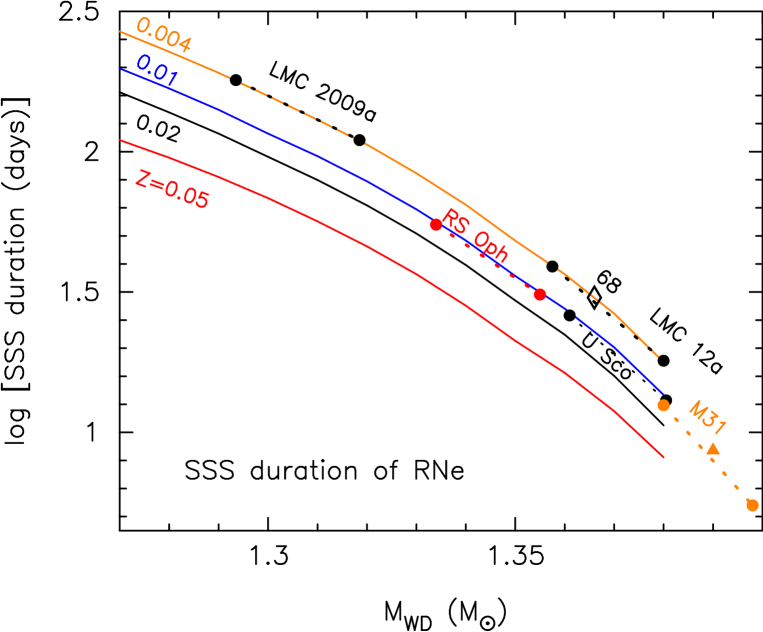
Figure 11: The calculated SSS durations of recurrent novae with various WD masses and heavy element contents of $Z=0.004$ (solid orange line), 0.01 (blue), 0.02 (black), and 0.05 (red). The dotted lines with large dots at the both sides indicate the SSS duration of individual nova, the name of which is beside the line. The left-side dot corresponds to the full width of SSS duration, $t_{\rm SSS}$, and the right-side dot the SSS duration after its highly variable phase ended, $t_{\rm SSS}^{*}$. The filled orange triangle indicates the 2016 outburst (shorter SSS) of M31N 2008-12a. The open black diamond shows $t_{\rm SSS}$ of LMC N 1968.

3.2 Comparison with observed SSS durations

Figure 11 summarizes the SSS durations calculated for various WD masses and metallicities. As explained in the previous section, the SSS duration quickly decreases as the WD mass increases toward the Chandrasekhar mass.

We also plot the six recurrent novae of a broad rectangular X-ray light curve. We place the galactic and M31 novae, i.e., U Sco, RS Oph and M31N 2008-12a, between the lines of $Z=0.01$ and $Z=0.02$, considering the recent estimates for the solar abundance of $Z=0.0138$ (Grevesse, 2019). For the three LMC novae, we adopt $Z=0.004$ as a typical value for the LMC stars.

These novae show high variability in their early X-ray phase. This variable phase has not been theoretically explained, so we do not know whether this phase corresponds to the end of the wind phase or post-wind phase in the theoretical models. Thus, we plot both the two durations, $t_{\rm SSS}$ and $t_{\rm SSS}^{*}$, at the left-edge dot and right-edge dot of each dotted line, respectively. The two single symbols represent LMC N 1968 (open black diamond) and M31N 2008-12a 2016 outburst (filled orange triangle) that have no corresponding $t_{\rm SSS}^{*}$.

The WD masses in these recurrent novae have been estimated by various methods. For RS Oph, the WD mass is estimated to be 1.35 $M_{\odot}$ from the optical light curve fitting with a composite model of the WD photosphere, irradiated accretion disk and companion (Hachisu et al., 2006b), and also to be 1.35 $M_{\odot}$ from fitting of the X-ray light curve after the highly variable phase ended (Hachisu et al., 2007). This value is consistent with our right-side point of the dotted line for RS Oph. This suggests that highly variable SSS phase is associated with the late wind phase rather than the phase after the wind stops. For U Sco, the WD mass is estimated to be $M_{\rm WD}=1.55\pm 0.24~{}M_{\odot}$ by Thoroughgood et al. (2001) from the double line orbital velocities, and about 1.37 $M_{\odot}$ by Hachisu & Kato (2000a) from the light curve fitting. These values are consistent with our dotted line. For M31N 2008-12a, a 1.38 $M_{\odot}$ WD is suggested from the theoretical models (Kato et al., 2015, 2016, 2017a). This value drops on the line for M31N 2008-12a in Figure 11.

For LMC novae, we fitted our SSS periods on the line of $Z=0.004$ in Figure 11. Hachisu & Kato (2018b) compared the X-ray and $V$ light curves of LMC N 2009a with theoretical light curve of $1.25~{}M_{\odot}$ with a neon rich composition (Ne nova 3 with $Z=0.02$: Figure 33a in Hachisu & Kato (2018b)). Note that this is a tentative fitting because no neon-enrichment is observed in LMC 2009a. Moreover, LMC N 2009a is an LMC member and we expect a lower metallicity ($Z<0.02$) and no substantial enrichment of neon. A nova evolution becomes shorter for a higher metallicity (Kato, 1997, 1999), thus, we expect a more massive WD than 1.25 $M_{\odot}$ for a lower metal environment. Thus, our value of $1.29-1.32~{}M_{\odot}$ in Figure 11 is reasonable. For LMC N 2012a, Hachisu & Kato (2018b) estimated the mass to be $1.37~{}M_{\odot}$ from a linear interpolation of the stretching factor. This value is consistent with our value in Figure 11.

In this way, our WD masses obtained from the SSS duration are consistent with the other theoretical and observational estimates. We conclude that the SSS duration of a recurrent nova is a good indicator of the WD mass if the X-ray light curve shows a broad rectangular shape.

4 Discussion

4.1 RS Oph and V2491 Cyg

Hachisu & Kato (2019a) compared the light curves of RS Oph and V2491 Cyg, and showed that $t_{\rm on}$ is almost the same, while $t_{\rm off}$ is very different (see their Figure 16). Figure 5 clarifies that this difference can be understood along with the increasing deviation of recurrent novae from classical novae toward a more massive WD. The WD mass of RS Oph has been estimated to be $1.35~{}M_{\odot}$ (see Section 3). Also the similar value, $M_{\rm WD}\sim 1.35~{}M_{\odot}$, is obtained in V2491 Cyg (Hachisu & Kato, 2019a) from the light curve fitting. In short, the WD mass is similar but the SSS duration is very different.

There are several reasons that result in a longer SSS period in recurrent novae than in classical novae having the same WD mass. The first is a longer variable period in the SSS phase. Both RS Oph and V2491 Cyg show a highly variable SSS phase, but RS Oph shows a much longer variable period. The second is the difference in the chemical composition of envelope. The ejecta is close to the solar composition in recurrent novae whereas the ejecta is enriched with heavy elements and deficient in hydrogen in classical novae (e.g., Table 1 in Hachisu & Kato (2006)). A smaller $X$ provides less nuclear fuel that results in a shorter nuclear-burning time. Also, the heavy element enrichment causes a smaller envelope mass. Thus, the SSS period is shorter. The last reason is high mass-accretion rates in recurrent novae that release larger gravitational energy per unit time. The WD core is heated and slightly expands. This makes the envelope mass larger in hydrostatic balance of SSS phase, and therefore the SSS phase becomes longer. To summarize, the SSS phases in recurrent novae are systematically longer than those in classical novae having the same WD mass because of the combination of these several effects.

For V2491 Cyg, Munari et al. (2011) obtained the composition of ejecta to be $X=0.573$, $Y=0.287$, and $Z=0.140$ by weight. Here, the individual elements are $X_{\rm N}=0.074$, $X_{\rm O}=0.049$, and $X_{\rm Ne}=0.015$. This heavy element enrichment strongly suggests that V2491 Cyg is not a recurrent nova but a classical nova, because such large amounts of heavy elements have not been detected in recurrent novae. Comparing with our model for RS Oph in Section 3, $X=0.56$ and $Z=0.02$ for the $1.35~{}M_{\odot}$, the hydrogen content is almost the same, but the heavy elements are much larger in V2491 Cyg. Even if the WD masses and $X$’s are the same between RS Oph and V2491 Cyg, the envelope mass when the winds stop is smaller for larger $Z$ (heavy element enrichment) and, as a result, the SSS phase of V2491 Cyg is much shorter.

4.2 T Pyx

T Pyx also shows a shorter SSS phase than the trend of recurrent novae as shown in Figure 5. Schaefer et al. (2010) examined the radial motion of ejecta knots around T Pyx and the quiescent $B$ magnitude decay since 1890 to 2009. They concluded that T Pyx experienced a first classical nova outburst around 1866 after a long period of very low mass-accretion rates, and it is currently staying in the period of very high mass-accretion rates, as indicated by several successive recurrent nova outbursts. In short, the mass accretion rate has long been very low before 1866, but increased after that. In such a case the WD interior is still cool, has not yet become hot. So the WD radius is possibly smaller than that of the hot WD corresponding to the high mass-accretion rates. Thus, the hydrogen-rich envelope mass is smaller than those of recurrent novae with the same WD mass. This is a possible explanation of the short SSS phase of T Pyx. We also point out that the duration of the SSS phase is close to the line for classical novae (blue line in Figure 5).

Figure 12: Comparison of the distribution of M31 novae with our empirical laws. The M31 novae are plotted with the black dots (data taken from Henze et al. (2014)). The solid black line indicates a relation made from the linear fit in the $(\log~{}t_{\rm on})$-$(\log~{}t_{\rm off})$ diagram by Henze et al. (2014). The other lines are the same as those in Figure 5, i.e., recurrent novae (orange), classical novae (blue), and $t_{\rm SSS}=t_{\rm off}$ (green). The red curved squares connected by the arrow indicate M31N 2010-10f; the upper square is by Henze et al. (2014) and the lower symbol is the position under our definition.

4.3 Comparison with M31 Classical Novae

In the present work, we concentrate on the recurrent novae and have not discussed much on classical novae. Here, we compare our results with the statistical work for classical novae appeared in M31 (Henze et al., 2011, 2014).

Figure 8(a) in Henze et al. (2014) shows the $t_{\rm on}$ - $t_{\rm off}$ diagram in which the M31 classical novae distribute around a line of Equation (1) with a relatively large scatter. This large scatter may be partly because of the sparse observation with telescopes and X-ray satellites that causes large ambiguities in the outburst day $t_{0}$, $t_{\rm on}$, and $t_{\rm off}$.

From Equation (1) we made a $t_{\rm SSS}$ - $t_{\rm off}$ relation and depicted it by the black line in Figure 12, as well as the SSS data for the 74 classical novae in M31 (black dots) taken from Henze et al. (2014). The black line is close to our line of recurrent novae rather than classical novae. The individual nova points, however, distribute widely and covers all the three lines.

There is a reason that we cannot directly compare these data with our results. It is the difference in the definition of $t_{\rm on}$ and $t_{\rm off}$. Henze et al. (2014) obtained the X-ray turn-on time, $t_{\rm on}$, as the middle of the last non-detection and the first detection time. Similarly, the turnoff time $t_{\rm off}$ is obtained as the mean of the last detection and non-detection times. On the other hand, our definition of turn on/off time is the time when the X-ray flux reaches one tenth of the peak flux. As a result, our $t_{\rm SSS}$ is likely to be shorter than Henze et al.’s if we have relatively dense observation.

For example, LMC N 2009a (Figure 2) is a well-observed nova in which the faint X-ray flux ($\sim$ one thousandth of the peak flux) is detected before and after the bright SSS phase. If we include these faint phase, we get an earlier $t_{\rm on}$, later $t_{\rm off}$, and much longer $t_{\rm SSS}$.

More exactly, we see the case of M31N 2010-10f in Figure 12. The black dot outlined by a curved red square represents the data in Henze et al. (2014), while the lower square is the one measured with our definition from the X-ray light curve presented by Henze et al. (2013) and Kato et al. (2013). Henze et al.’s value is larger than ours by a factor of 5.7, because they counted the post outburst faint X-rays.

In this way, it is hard to directly compare our results with the statistical data by Henze et al. (2014). To draw a qualitative conclusion we need to adopt the same definition of the X-ray phase.

5 Conclusions

We examined supersoft X-ray light curves of seven recurrent novae and one candidate. Our main results are summarized as follows.

1. Six novae out of eight, M31N 2008-12a, LMC N 1968, U Sco, LMC N 2012a, RS Oph, and LMC N 2009a, show a broad rectangular X-ray light curve shape. The X-ray phase is highly variable in the first half period. The optical light curve shows a plateau during the SSS phase that indicates the presence of a large irradiated accretion disk.

2. These six novae show a common proportionality relation between the SSS duration and total nova duration, $t_{\rm SSS}=0.70~{}t_{\rm off}$. If we exclude the highly variable phase from the SSS phase, the relation is $\log~{}t_{\rm SSS}^{*}=1.08~{}(\log~{}t_{\rm off}-1.2)+0.7$.

3. The other two novae, V745 Sco and T Pyx, show a narrow triangular shape of X-ray light curve without a highly-variable phase. Their SSS phases are shorter than the proportionality relation of $t_{\rm SSS}=0.70~{}t_{\rm off}$. The $t_{\rm SSS}$ of V745 Sco suddenly drops from the line of $t_{\rm SSS}=0.70~{}t_{\rm off}$ at the shortest limit of $t_{\rm off}$. The $t_{\rm SSS}$ of T Pyx is slightly below the line of $t_{\rm SSS}=0.70~{}t_{\rm off}$ at the longer edge of $t_{\rm off}$ for recurrent novae, and rather close to the $t_{\rm SSS}$-$t_{\rm off}$ relation for classical novae proposed by Hachisu & Kato (2010). The resemblance to classical novae is consistent with the observational suggestion that T Pyx has recently become a recurrent nova in 1866 and had undergone a very long quiescent phase before that.

4. The 2016 outburst of M31N 2008-12a shows a shorter $t_{\rm SSS}$ and $t_{\rm off}$ than those of the other year’s, the position of which is located in the middle of usual M31N 2008-12a and V745 Sco. We consider the 2016 outburst (shorter duration) to be the key to examine whether V745 Sco is the shortest end of the bending line near the edge or merely an exception to the proportionality relation.

5. We present theoretical SSS durations calculated for recurrent novae with various WD masses and stellar metallicities ($Z=$0.004, 0.01, 0.02 and 0.05). Comparing the observed SSS phase with the model calculation, we estimate the WD mass for the five recurrent novae with a broad rectangular SSS shape. These WD masses are in good agreement with those estimated from the other methods. The duration of the SSS phase of a recurrent nova is a good indicator of the WD mass.

We are grateful to Martin Henze for providing us the M31 nova data. We also thank the anonymous referee for useful comments that improved the manuscript.

Figure 13: (a) The X-ray turn-on time, (b) X-ray turnoff time, and (c) duration of the supersoft X-ray phase of classical novae against the WD mass. The different color indicates the different chemical composition of typical classical novae (Hachisu & Kato, 2010). From upper to lower. Gray line: Ne nova 3 ($X,~{}Y,~{}X_{\rm CNO},~{}X_{\rm Ne})$=(0.65, 0.27, 0.03, 0.03). Blue line: Ne nova 2 (0.55, 0.3, 0.1, 0.03). Orange line: CO nova 4 (0.55, 0.23, 0.2, 0.0). Red line: CO nova 3 (0.45, 0.18, 0.35, 0.0). For all the cases the heavy element abundance is assumed to be $Z=0.02$ and $X+Y+X_{\rm CNO}+X_{\rm Ne}+Z=1$.

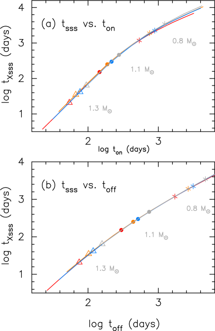
Figure 14: Duration of the supersoft X-ray phase of classical novae against (a) X-ray turn-on time, and (b) X-ray turnoff time. The color corresponds to the model of the same color in Figure 13. The positions of the three WD masses are indicated on each line with the same color as the line. Open triangles: 1.3 $M_{\odot}$. Dots: 1.1 $M_{\odot}$. Asterisks: 0.8 $M_{\odot}$.

Appendix A Theoretical relation of $t_{\rm SSS}-t_{\rm off}$ for classical novae

The decay phase of a nova can be followed by a sequence of steady-state and static envelope solutions (Kato & Hachisu, 1994). Hachisu & Kato (2010) calculated $t_{\rm on}$ and $t_{\rm off}$ for various WD masses and chemical compositions. The SSS duration is calculated by $t_{\rm SSS}=t_{\rm off}-t_{\rm on}$. Figure 13 shows $t_{\rm on}$, $t_{\rm off}$, and $t_{\rm SSS}$ for various WD masses and different chemical compositions of hydrogen-rich envelopes. The four lines represent typical compositions of novae (Hachisu & Kato, 2010); Ne nova 3 ($X,~{}Y,~{}X_{\rm CNO},~{}X_{\rm Ne})=(0.65,0.27,0.03,0.03)$ (gray line), Ne nova 2 $(0.55,0.3,0.1,0.03)$ (blue line), CO nova 4 $(0.55,0.23,0.2,0.0)$ (orange line), and CO nova 3 $(0.45,0.18,0.35,0.0)$ (red line). For all the cases, we assume $Z=0.02$ and $X+Y+Z+X_{\rm CNO}+X_{\rm Ne}=1$.

Kato & Hachisu (1994); Hachisu & Kato (2006, 2010) clarified that the nova evolution speed depends strongly on the WD mass and weakly on the chemical composition. As in Figure 13, a nova on a more massive WD evolves faster so both the $t_{\rm on}$ and $t_{\rm off}$ times are smaller. For the same WD mass, the nova evolution is faster for smaller $X$ and for larger $X_{\rm CNO}$. Thus, both the $t_{\rm on}$ and $t_{\rm off}$ are smaller.

Figure 14 shows the SSS duration of the same models as in Figure 13, but against the X-ray (a) turn-on and (b) turnoff time. All the four lines converge into one. Although the lines are almost converged, the WD mass associated with each line is different. The points corresponding to the $0.8~{}M_{\odot}$, $1.1~{}M_{\odot}$ and $1.35~{}M_{\odot}$ are indicated on each line. For the same WD mass, the SSS duration is longer for a larger hydrogen content $X$.

Figures 5 and 6 show the relations between $t_{\rm on}$, $t_{\rm off}$, and $t_{\rm SSS}$ taken from Figure 14. The line is a combination of CO nova 3 ($\leq 1.05~{}M_{\odot}$) and Ne nova 2 ($\geq 1.05~{}M_{\odot}$) as a representative of typical novae (Figure 22 in Hachisu & Kato (2019b)). These two lines are smoothly connected with a small overlap around $\log~{}t_{\rm SSS}$ (days) =2.4. Even if we adopt the other chemical composition, this line hardly changes as shown in Figure 14.

References

- Bode et al. (2016) Bode, M. F., Darnley, M. J., Beardmore, A. P., et al. 2016, ApJ, 818, 145
- Chomiuk et al. (2014) Chomiuk, L, Nelson, T., Mukai, K. et al. 2014, ApJ, 788, 130
- Darnley et al. (2016) Darnley, M. J., et al. 2016, ApJ, 833, 149
- Darnley et al. (2015) Darnley, M. J., et al. 2015, A&A, 580, A45
- Drake et al. (2016) Drake, J., J., Delgado, L., Laming, J. M. et al. 2016, ApJ, 825, 95
- Evans et al. (2009) Evans, P. A., Beardmore, A. P., Page, K. L., et al. 2009, MNRAS, 397, 1177
- Grevesse (2019) Grevesse, N. 2019, Bulletin de la Société Royale des Siences de Liége, 88, 5
- Hachisu & Kato (2000a) Hachisu, I., & Kato, M. 2000, ApJ, 528, L97
- Hachisu & Kato (2000b) Hachisu, I., & Kato, M. 2000, ApJ, 534, L189
- Hachisu & Kato (2006) Hachisu, I., & Kato, M. 2006, ApJS, 167, 59
- Hachisu & Kato (2007) Hachisu, I., & Kato, M. 2007, ApJ, 662, 552
- Hachisu & Kato (2009) Hachisu, I., & Kato, M. 2009, ApJ, 694, L103
- Hachisu & Kato (2010) Hachisu, I., & Kato, M. 2010, ApJ, 709, 680
- Hachisu & Kato (2015) Hachisu, I., & Kato, M. 2015, ApJ, 798, 76
- Hachisu & Kato (2016a) Hachisu, I., & Kato, M. 2016, ApJ, 816, 26
- Hachisu & Kato (2016b) Hachisu, I., & Kato, M. 2016, ApJ, 824, 22
- Hachisu & Kato (2016c) Hachisu, I., & Kato, M. 2016, ApJS, 223, 21
- Hachisu & Kato (2018a) Hachisu, I., & Kato, M. 2018a, ApJ, 858, 108
- Hachisu & Kato (2018b) Hachisu, I., & Kato, M. 2018b, ApJS, 237, 4
- Hachisu & Kato (2019a) Hachisu, I., & Kato, M. 2019a, ApJS, 241, 4
- Hachisu & Kato (2019b) Hachisu, I., & Kato, M. 2019b, ApJS, 242, 18
- Hachisu et al. (2006b) Hachisu, I., Kato, M., Kiyota, S., et al. 2006b, ApJ, 651, L141
- Hachisu et al. (2007) Hachisu, I., Kato, M., & Luna, G. J. M. 2007, ApJ, 659, L153
- Hachisu et al. (2016) Hachisu, I., Saio, H., & Kato, M. 2016, ApJ, 824, 22
- Henze et al. (2015) Henze, M., Ness, J.-U., Darnley, M., et al. 2015, A&A, 580, 46
- Henze et al. (2018) Henze, M., Darnley, M., Williams, S. C. et al. 2018, ApJ, 857, 68
- Henze et al. (2013) Henze, M., Pietsch, W., Haberl, F., et al. 2013, 549, 120
- Henze et al. (2014) Henze, M., Pietsch, W., Habert, F., Della Valle, M., Sala, G, Hatzidimitriou, D., Hofmann, F., Hernanz, M. et al. 2014, A&A, 563, A2
- Henze et al. (2011) Henze, M., Pietsch, W., Haberl, F., Hernanz, M., Sala, G., Hatzidimitriou, D., Della Valle, M., Rau, A. et al. 2011, A&A, 533, A52
- Kato (1997) Kato, M. 1997, PASJ, 113, 121
- Kato (1999) Kato, M. 1999, PASJ, 51, 525
- Kato (2011) Kato, M. 2011, in Binary Paths to Type Ia Supernovae Explosions, IAU symposium no. 281, ed. R. Di Stefano, M. Orio, & M. Moe (Cambridge: Cambridge University Press), 172
- Kato & Hachisu (1994) Kato, M., & Hachisu, I. 1994, ApJ, 437, 802
- Kato & Hachisu (2012) Kato, M., & Hachisu, I. 2012, Bull.Astr.Soc,India, 40, 393
- Kato et al. (2013) Kato, M., Hachisu, I., & Henze, M. 2013, ApJ, 779, 19
- Kato et al. (2017) Kato, M., Hachisu, I., & Saio, H. 2017, in The Golden Age of Cataclysmic Variables and Related Objects - IV, ed. F. Giovannelli et al. (Trieste: SISSA PoS), 315, 56
- Kato et al. (2014) Kato, M., Saio, H., Hachisu, I., & Nomoto, K. 2014, ApJ, 793, 136
- Kato et al. (2015) Kato, M., Saio, H., & Hachisu, I. 2015, ApJ, 808, 52
- Kato et al. (2017a) Kato, M., Saio, H., & Hachisu, I. 2017a, ApJ, 838, 153
- Kato et al. (2018) Kato, M., Saio, H., & Hachisu, I., 2008, ApJ, 863, 125
- Kato et al. (2016) Kato, M., Saio, H., Henze, M. et al. 2016, ApJ, 830, 40
- Kuin et al. (2020) Kuin, N.P., Page, K.L., Mróz, P., Darnley, M. J., Shore, S. N. et al 2020, MNRAS, 491, 655
- Munari et al. (1990) Munari, U., Margoni, R., & Stagni, R. 1990, MNRAS, 242, 653
- Munari et al. (2011) Munari, U., Siviero, A., and Dallaporta, S. 2011, New Astronomy, 16, 209
- Ness et al. (2012) Ness, J.-U., Schaefer, B. E., Dobrotka, A., et al. 2012, ApJ, 745, 43
- Nelson et al. (2012) Nelson, T., Donato, D., Mukai, K., Sokoloski, J., & Chomiuk, L. 2012, ApJ, 748, 43,
- Nelson et al. (2014) Nelson, T., Chomiuk, L. Roy, N. et al. (2014) ApJ, 785,78
- Ness et al. (2011) Ness, J.-U., Osborne, J.P., Dobrotka, A., et al. ApJ, 733, 70
- Orio et al. (2013) Orio, M., Behar, E., Gallagher, J. et al. 2013, MNRAS, 429, 1342
- Orio et al. (2015) Orio, M., Rana, V., Page, K. L., Sokoloski, J., & Harrison, F. 2015, MNRAS, 448, L35
- Osborne et al. (2011) Osborne, J. P., Page, K. L., Beardmore, A.P., et al. 2011, ApJ, 727, 124
- Page et al. (2010) Page, K.L., Osborne, J.P., Evans, P.A. et al., 2010, MNRAS, 401, 121
- Page et al. (2015) Page, K.L., Osborne, J.P., Kuin, N.P.M. et al., 2015, MNRAS, 454, 3108
- Payne-Gaposchkin (1957) Payne-Gaposchkin, C. 1957, The galactic Novae (Amsterdam: North-Holland)
- Sala & Hernanz (2005) Sala, G., & Hernanz, M. 2005, A&A, 439, 1061
- Schaefer (2010) Schaefer, B. E. 2010, ApJS, 187, 275
- Schaefer et al. (2010) Schaefer, B. E., Pagnotta, A., & Shara, M. M. 2010, ApJ, 708 381
- Schaefer et al. (2013) Schaefer, B.,E., Landolt, A.U., Linnolt, M. et al. 2013, ApJ, 773, 55
- Schwarz et al. (2015) Schwarz, G. J., Shore, S. N., Page, K. L., et al. 2015, AJ, 149, 95
- Strope et al. (2010) Strope, R., Schaefer, B. E., & Henden, A. A. 2010, AJ, 140, 34
- Thoroughgood et al. (2001) Thoroughgood, T. D., Dhillon, V. S., Littlefair, S. P., Marsh, T. R., & Smith, D. A. 2001, MNRAS, 327, 1323
- Walter et al. (2012) Walter, F. M., Battisti, A., Towers, S. E., Bond, H. E., & Stringfellow, G. S. 2012, PASP, 124, 1057
- Wolf et al. (2013) Wolf, W. M., Bildsten, L., Brooks, J., & Paxton, B. 2013, ApJ, 777, 136,