Limit theorems for Lévy flights
on a 1D Lévy random medium

Abstract

We study a random walk on a point process given by an ordered array of points $(\omega_{k},\,k\in\mathbb{Z})$ on the real line. The distances $\omega_{k+1}-\omega_{k}$ are i.i.d. random variables in the domain of attraction of a $\beta$-stable law, with $\beta\in(0,1)\cup(1,2)$. The random walk has i.i.d. jumps such that the transition probabilities between $\omega_{k}$ and $\omega_{\ell}$ depend on $\ell-k$ and are given by the distribution of a $\mathbb{Z}$-valued random variable in the domain of attraction of an $\alpha$-stable law, with $\alpha\in(0,1)\cup(1,2)$. Since the defining variables, for both the random walk and the point process, are heavy-tailed, we speak of a Lévy flight on a Lévy random medium. For all combinations of the parameters $\alpha$ and $\beta$, we prove the annealed functional limit theorem for the suitably rescaled process, relative to the optimal Skorokhod topology in each case. When the limit process is not càdlàg, we prove convergence of the finite-dimensional distributions. When the limit process is deterministic, we also prove a limit theorem for the fluctuations, again relative to the optimal Skorokhod topology.
Mathematics Subject Classification (2020): 60G50; 60G55; 60F17; 82C41; 60G51
Keywords: Random walk on point process; Lévy random medium; Lévy flights; Stable distributions; Anomalous diffusion; Stable processes.

1 Introduction

The expression ‘Lévy random medium’ indicates a stochastic point process, in some space, where the distances between nearby points have heavy-tailed distributions. Processes of this kind have been receiving a surge of attention, of late, both in the physical and mathematical literature; cf., respectively, [BFK, S, BCV, BDLV, ZDK, VBB] and [BCLL, BLP, MS, Za]. They model a variety of situations that are of interest in the sciences. In particular, they are used as supports for various kinds of random walks, in order to study phenomena of anomalous transport and anomalous diffusion. An incomplete list of general or recent references on this topic includes [SZF, KRS, CGLS, ZDK, ACOR, ROAC, ROAP].

The random medium that we consider in this paper is perhaps the most natural choice for a Lévy random medium in the real line: a sequence of random points $\omega=(\omega_{k},\,k\in\mathbb{Z})$, where $\omega_{0}=0$ and the nearest-neighbor distances $\zeta_{k}=\omega_{k+1}-\omega_{k}$ are i.i.d. variables in the normal domain of attraction of a $\beta$-stable variable, with $\beta\in(0,1)\cup(1,2)$. Here $\beta$ is the index of the stable distribution, not the skewness parameter, which equals 1 because $\zeta_{k}>0$.

A random walk $Y=(Y_{n},\,n\in\mathbb{N})$ takes place on $\omega$ according to the following rule. Independently of $\omega$, there exists a random walk $S=(S_{n},\,n\in\mathbb{N})$ on $\mathbb{Z}$ with $S_{0}=0$ and i.i.d. increments in the normal domain of attraction of an $\alpha$-stable variable, with $\alpha\in(0,1)\cup(1,2)$. We define $Y_{n}:=\omega_{S_{n}}$. This means that the process $Y$ performs the same jumps as $S$, but on the marked points $\omega_{k}$ instead of $\mathbb{Z}$. For example, if a realization of $S$ is $(0,3,-1,\ldots)$, the process $Y$ starts at the origin of $\mathbb{R}$, then jumps to the third marked point to the right of $0$, then to the first marked point to the left of $0$, and so on. In other words, $S$ drives the dynamics of $Y$ on the Lévy medium. For this reason we call it the underlying random walk.

Our process of interest is $Y$. We may describe it as a Lévy flight on a one-dimensional Lévy random medium. This phrase is borrowed from the physical literature, where the term ‘Lévy flight’ usually indicates a discrete-time random walk with long-tailed instantaneous jumps. This is in contrast to a ‘Lévy walk’, which in general designates a persistent, continuous- or discrete-time, random walk with long-tailed trajectory segments that are run at constant finite speed [ZDK]. A Lévy walk is often seen as an interpolation of a Lévy flight. For example, an important process from the standpoint of applications is $X:=(X(t),\,t\in[0,+\infty))$, the unit-speed interpolation of $Y$. This means that, for any realization of $Y$, a trajectory of $X$ starts at the origin and visits all the points $Y_{n}$ in the given order, traveling between them with velocity $1$ or $-1$, depending on $Y_{n+1}$ being to the right or to the left of $Y_{n}$, respectively. The walk $X$ is a generalization of a system that first appeared in the physical literature 20 years ago with the name Lévy-Lorentz gas [BFK] (more precisely, the Lévy-Lorentz gas is the case where the underlying random walk is simple). It was devised as a one-dimensional toy model for the study of anomalous diffusion in porous media [L, BFK, BCV]. See [BCLL, BLP, Za] for recent mathematical results.

There are several reasons to study our Lévy flight on random medium. The most self-serving, on the part of the present authors, is to build a basis to investigate the properties of the associated Lévy walk, as described above (see the proofs in [BCLL, BLP]). Also, $Y$ can be thought of as the limit of a continuous-time random walk with resting times on the points $\omega_{k}$, when the ratio between the speed of the walker and the typical resting time diverges. This can be used to model a variety of situations where a given dynamics is very fast compared to its “decision times”, e.g., electronic signal on a network whose nodes act as relatively slow processing stations; human mobility (assuming, as is often the case, that resting times are substantially longer than travel times); etc. This particular model aside, there is no lack of general motivation for the study of random walks on points processes, especially in light of the fact that the topic is regrettably less developed than others in the field of random walks, with the exception perhaps of random walks on percolation clusters et similia. For some interesting lines of research see, e.g., [CF, CFP, K, BR, Z, R] and references therein. A recent paper which we extend with the present work is [MS].

In this paper we give annealed limit theorems for $Y$ in all cases $\alpha,\beta\in(0,1)\cup(1,2)$, identifying in each case both the scale $n^{\gamma}$ whereby

$$\left(\frac{Y_{\lfloor nt\rfloor}}{n^{\gamma}}\,,\,t\in[0,+\infty)\right)$$ (1)

converges to a non-null limit, and the limit process. In all cases we prove the optimal, or at least morally optimal, functional limit theorem, meaning that we show distributional convergence of the process with respect to (w.r.t.) the strongest Skorokhod topology that applies there. There are cases in which there can be no convergence in the $J_{1}$ or $M_{1}$ topologies: in such cases we prove convergence w.r.t. $J_{2}$. When the limit process is not càdlàg (or càglàd) we show convergence of the finite-dimensional distributions. Finally, in the cases where the limit of (1) is deterministic, we prove a functional limit theorem for the corresponding fluctuations, again relative to the optimal topology.

The paper is organized as follows. In Sections 2.1 and 2.2 we describe the model and set the notation for the $J_{1}$ and $J_{2}$ Skorokhod topologies on spaces of càdlàg/càglàd functions; in Section 2.3 we lay out basic limit theorems for the underlying random walk $S$ and the random medium $\omega$; in Section 2.4 we present our main results. Finally, Section 3 contains all the proofs of the main theorems.

Acknowledgments.

We thank Ward Whitt for discussing with us the issue of the $J_{2}$-continuity of the addition map (cf. end of Section 3.4). This work was partly supported by the joint UniBo-UniFi-UniPd project “Stochastic dynamics in disordered media and applications in the sciences”. A. Bianchi is partially supported by the PRIN Grant 20155PAWZB “Large Scale Random Structures” (MIUR, Italy) and by the BIRD project 198239/19 “Stochastic processes and applications to disordered systems” (UniPd). M. Lenci is partially supported by the PRIN Grant 2017S35EHN “Regular and stochastic behaviour in dynamical systems” (MIUR, Italy). E. Magnanini thanks the Department of Mathematics of Università di Bologna, to which she was affiliated when most of this work was done.

2 Model and Results

2.1 Setup

As mentioned in the introduction, the Lévy flight on random medium that we consider is a random walk performed over the points of a certain random point process. We proceed to define all the necessary constructions.

Random medium.

Let $\zeta:=\left(\zeta_{i},\,i\in\mathbb{Z}\right)$ be a sequence of i.i.d. positive random variables. We assume that the law of $\zeta_{i}$ belongs to the normal basin of attraction of a $\beta$-stable distribution, with $\beta\in(0,1)\cup(1,2)$. In the case $\beta\in(0,1)$, this means that, as $n\to+\infty$,

$$\frac{1}{n^{1/\beta}}\sum_{i=1}^{n}\zeta_{i}\xrightarrow{\>\>\text{d}\>\>}Z^{(\beta)}_{1},$$ (2)

where $Z^{(\beta)}_{1}$ is a stable variable of index $\beta$ and skewness parameter 1 (because $\zeta_{i}>0$). In the case $\beta\in(1,2)$ we have instead

$$\frac{1}{n^{1/\beta}}\sum_{i=1}^{n}(\zeta_{i}-\nu)\xrightarrow{\>\>\text{d}\>\>}\tilde{Z}^{(\beta)}_{1},$$ (3)

for a stable variable $\tilde{Z}^{(\beta)}_{1}$ of index $\beta$. In this case, necessarily, $\nu$ is the expectation of $\zeta_{i}$ and the skewness parameter is 0.

The random medium associated to $\left(\zeta_{i},i\in\mathbb{Z}\right)$ is defined to be:

$$\omega_{0}=0,\qquad\omega_{k}=\begin{cases}\sum_{i=1}^{k}\zeta_{i}&\text{ if }k>0,\\ 0&\text{ if }k=0,\\ -\sum_{i=k}^{-1}\zeta_{i}&\text{ if }k<0.\end{cases}$$ (4)

This determines a point process $\omega:=\left(\omega_{k},\,k\in\mathbb{Z}\right)$ on $\mathbb{R}$ that we call Lévy random medium to emphasize the fact that the distribution of $\zeta_{i}$ has a heavy tail. Each point $\omega_{k}$ will be called a target. In other words, the distances between neighboring targets are drawn according to independent random variables $\zeta_{i}$.

Underlying random walk.

We consider a $\mathbb{Z}$-valued random walk $S:=(S_{n},\,n\in\mathbb{N})$, with $S_{0}=0$ and i.i.d. increments $\xi_{i}:=S_{i}-S_{i-1}$ that are independent of $\zeta$ (and thus of $\omega$). In other words, $S$ is given by

$$S_{0}=0,\qquad S_{n}=\sum_{i=1}^{n}\xi_{i}\quad\text{ for }n\in\mathbb{Z}^{+}.$$ (5)

The law of $\xi_{i}$ belongs to the normal basin of attraction of an $\alpha$-stable distribution, with $\alpha\in(0,1)\cup(1,2)$. This means that convergences analogous to those given in (2) and (3) apply to the $\xi_{i}$, with limit random variables denoted by $W^{(\alpha)}_{1}$ and $\widetilde{W}^{(\alpha)}_{1}$, respectively. We will refer to $S$ as the underlying random walk.

Random walk on the random medium.

The random walk on the random medium $Y:=(Y_{n},\,n\in\mathbb{N})$ is defined to be:

$$Y_{n}:=\omega_{S_{n}},\quad n\in\mathbb{N}.$$ (6)

In other words, $Y$ performs the same jumps as $S$, but on the points of $\omega$; see Figure 1 for a hands-on explanation. In the following we will focus on the derivation of the asymptotic law of $Y$, under suitable scaling, with respect to the probability measure $\mathbb{P}$ governing the entire system (medium and dynamics). This is sometimes referred to as the annealed or averaged law of $Y$.

Figure 1: Top: A realization of the underlying random walk $S$ on $\mathbb{Z}$. Middle: A realization of the random medium $\omega$, with inter-distances given by $\zeta_{i}$. Bottom: The corresponding process $Y$ jumps between the targets $\omega$ according to the walk $S$.

Before recalling certain basic facts about the processes $\omega$ and $S$, and stating our main results on the process $Y$, let us fix the notation for spaces of càdlàg functions endowed with certain Skorokhod topologies.

2.2 Càdlàg functions and Skorokhod topologies

Given $I$, an interval or a half-line contained in $\mathbb{R}^{+}:=[0,+\infty)$, we denote by $\mathcal{D}(I)\equiv\mathcal{D}(I;\mathbb{R})$ the space of all càdlàg functions $f:I\longrightarrow\mathbb{R}$, where we recall that these are right-continuous functions with left limits at all points of their domain. If $I$ is an interval or a half-line intersecting $(-\infty,0)$, or $I=\mathbb{R}$, we consider a less customary function space: $\mathcal{D}(I)$ is the space of all functions $f:I\longrightarrow\mathbb{R}$ such that $s\mapsto f(s)$ is càdlàg for $s\geq 0$ and $s\mapsto f(-s)$ is càdlàg for $s\geq 0$ (in other words, the restriction of $f$ to $I\cap(-\infty,0]$ is càglàd). Notice that this implies that $f$ is continuous at 0. We also use the abbreviations $\mathcal{D}^{+}\equiv\mathcal{D}(\mathbb{R}^{+})$ and $\mathcal{D}\equiv\mathcal{D}(\mathbb{R})$. Lastly, we denote by $\mathcal{D}_{0}$ and $\mathcal{D}^{+}_{0}$ the subspaces of nondecreasing functions of $\mathcal{D}$ and $\mathcal{D}^{+}$, respectively.

In this section we introduce two notions of distance/topology that turn out to be crucial in the following. A complete treatment of these topologies can be found, e.g., in [W2, Sections 3.3. & 11.5].

Definition 2.1.

Let $I$ be a bounded interval (which can be closed, open or half-open). For $f,g\in\mathcal{D}(I)$, denote

$$d_{J_{1},I}(f,g):=\inf_{\lambda:I\to I}\max\left\{\sup_{t\in I}|f\circ\lambda(t)-g(t)|\>,\>\sup_{t\in I}|\lambda(t)-t|\right\},$$ (7)

where the infimum is taken over all increasing homeomorphisms $\lambda:I\longrightarrow I$. This defines a distance on $\mathcal{D}(I)$, which we refer to as the $J_{1}$ or $J_{1}(I)$ distance.

This metric induces a topology and a notion of limit in $\mathcal{D}(I)$ which can be reformulated as follows: given $(f_{n})_{n\in\mathbb{N}}$ and $f$ in $\mathcal{D}(I)$, the sequence $f_{n}$ is said to converge to $f$ in the $J_{1}$ topology, and we write

$$f_{n}\to f\qquad\text{in }(\mathcal{D}(I),J_{1}),$$ (8)

as $n\to\infty$, if there exists a sequence of increasing homeomorphisms ${\lambda}_{n}:I\longrightarrow I$ such that

$$\lim_{n\to\infty}\, \sup_{t\in I}|f_{n}\circ\lambda_{n}(t)-f(t)|=0,$$ (9)

$$\lim_{n\to\infty}\, \sup_{t\in I}|\lambda_{n}(t)-t|=0.$$ (10)

Definition 2.2.

If $I\subset\mathbb{R}$ is a half-line, say $I=[a,+\infty)$, and $(f_{n})_{n\in\mathbb{N}}$, $f$ are functions of $\mathcal{D}(I)$, we say that $f_{n}\to f$ in $(\mathcal{D}(I),J_{1})$, for $n\to\infty$, if, for all $T>a$ such that $f$ is continuous at $T$,

$$f_{n}\to f\qquad\text{in }(\mathcal{D}([a,T]),J_{1}).$$ (11)

The analogous definition is given for $I=(a,+\infty)$ or $I=(-\infty,a]$, etc. If $I=\mathbb{R}$, we say that $f_{n}\to f$ in $(\mathcal{D},J_{1})$ if, for all $T>0$ such that $f$ is continuous at $T$ and $-T$,

$$f_{n}\to f\qquad\text{in }(\mathcal{D}([-T,T]),J_{1}).$$ (12)

The above definition defines a $J_{1}$ topology on $\mathcal{D}(I)$, in all cases where $I$ is a half-line or the entire $\mathbb{R}$. It is easy to write a metric that generates the $J_{1}(I)$ topology (see [W1, Section 2]).

Remark 2.1.

Although there are good reasons of convenience for using spaces of functions that are càdlàg on $\mathbb{R}^{+}$ and càglàd on $\mathbb{R}^{-}$ (see Section 3), some readers may find this choice odd and prefer to always work with càdlàg functions, even for domains $I$ intersecting $(-\infty,0)$. Clearly, to any $f\in\mathcal{D}(I)$ as defined earlier there corresponds a unique càdlàg version

$$f_{\mathrm{cadlag}}(t):=\lim_{s\to t^{+}}f(s).$$ (13)

For any bounded $I$, it is easy to see that $d_{J_{1},I}(f_{\mathrm{cadlag}},g_{\mathrm{cadlag}})=d_{J_{1},I}(f,g)$.

Remark 2.2.

In this paper the only two cases in which we work with $I$ intersecting $(-\infty,0)$ are $I=[-M,M]$ and $I=\mathbb{R}$. In both cases we only deal with functions $f$ such that $f(0)=0$. It is easy to see that, under such additional condition, it is no loss of generality to require that the homemorphism ${\lambda}$ fixes 0, i.e., ${\lambda}(0)=0$. This makes it clear that, in such cases, $f_{n}\to f$ in $(\mathcal{D}([-M,M]),J_{1})$ if and only if both $f_{n}\to f$ and $f_{n}(-\>\cdot)\to f(-\>\cdot)$ in $(\mathcal{D}([0,M]),J_{1})$. Here $f(-\>\cdot)$ denotes the function $t\mapsto f(-t)$.

If we think of $f_{n}$ as describing the spatial motion of some particle, the function ${\lambda}:I\longrightarrow I$ of (7) is sometimes called the time change. Requiring the time change to be a homeomorphism is occasionally too strong a condition. One has a weaker topology if they only require that ${\lambda}$ be a (possibly discontinuous) bijection:

Definition 2.3.

If $I$ is a bounded interval and $f,g\in\mathcal{D}(I)$, the $J_{2}$ or $J_{2}(I)$ distance $d_{J_{2},I}(f,g)$ is defined as in the r.h.s. of (7), but with the infimum taken over all bijections $\lambda:I\longrightarrow I$. The notions of $J_{2}$-convergence in all cases of $I$ are derived as seen earlier for $J_{1}$.

Remark 2.3.

It is a known and easy-to-prove fact that, if $I_{0}\subseteq I$ is an interval at positive distance from the discontinuities of $f$, and $f_{n}\to f$ in $(\mathcal{D}(I),J_{i})$, for either $i=1$ or $i=2$, then $\sup_{t\in I_{0}}|f_{n}(t)-f(t)|\to 0$.

Remark 2.4.

The definition of limit in $(\mathcal{D}([a,+\infty)),J_{i})$ ($i=1,2$) amounts to checking that $f_{n}\to f$ in $(\mathcal{D}([a,T]),J_{i})$, for all $T>a$ such that $f$ is continuous at $T$, see (11). With the help of the previous remark, it is easy to see that this is tantamount to checking that $f_{n}\to f$ in $(\mathcal{D}([a,T)),J_{i})$, for all $T>a$ such that $f$ is continuous at $T$. In the remainder (see for example Section 3.3) we will liberally switch between the two conditions, as is more convenient.

2.3 Limit processes for $\omega$ and $S$

We now recall some elementary functional limit theorems for suitable rescalings of the processes $\omega$ and $S$, cf. (4) and (5).

By definition, for all $k\in\mathbb{Z}$, $\omega_{k}$ is a sum of $|k|$ i.i.d. random variables $\zeta_{i}$ in the normal domain of attraction of a $\beta$-stable distribution. We first deal with the case $\beta\in(0,1)$. For every $s\in\mathbb{R}$ we define

$$\hat{\omega}^{(n)}(s):=\begin{dcases}\frac{\omega_{\lfloor ns\rfloor}}{n^{1/\beta}}&\text{ if }s\geq 0,\\[4.0pt] \frac{\omega_{\lceil ns\rceil}}{n^{1/\beta}}&\text{ if }s<0.\end{dcases}$$ (14)

Let $(Z^{(\beta)}_{\pm}(s),\,s\geq 0)$ be two i.i.d. càdlàg Lévy $\beta$-stable processes such that $Z^{(\beta)}_{\pm}(0)=0$ and $Z^{(\beta)}_{\pm}(1)$ is distributed like $Z^{(\beta)}_{1}$, as introduced in (2) (these two conditions uniquely determine the common distribution of the processes). Set

$$Z^{(\beta)}(s):=\begin{dcases}Z^{(\beta)}_{+}(s)&\mbox{ if }s\geq 0,\\ -Z^{(\beta)}_{-}(-s)&\mbox{ if }s<0.\end{dcases}$$ (15)

Then (see, e.g., [W2, Section 4.5.3]), as $n\to\infty$,

$$\hat{\omega}^{(n)}\xrightarrow{\>\>\text{d}\>\>}Z^{(\beta)}\IfEqCase{1}{{1}{\qquad\text{in }(\mathcal{D},J_{1})}{2}{\qquad\text{in }(\mathcal{D},J_{2})}}[].$$ (16)

When $\beta\in(1,2)$, the average distance $\nu:=\mathbb{E}[\zeta_{i}]$ between successive targets is finite and positive by assumption. So, at first order, a Strong Law of Large Numbers holds. More in detail, setting

$$\bar{\omega}^{(n)}(s):=\begin{dcases}\frac{\omega_{\lfloor ns\rfloor}}{n}&\text{ if }s\geq 0,\\[4.0pt] \frac{\omega_{\lceil ns\rceil}}{n}&\text{ if }s<0,\end{dcases}$$ (17)

we have

$$\bar{\omega}^{(n)}\xrightarrow{\>\>\text{a.s.}\>\>}\nu\hskip 1.00006pt\mathrm{id}\IfEqCase{1}{{1}{\qquad\text{in }(\mathcal{D},J_{1})}{2}{\qquad\text{in }(\mathcal{D},J_{2})}}[],$$ (18)

as $n\to\infty$. Here and in the rest of the paper $\mathrm{id}$ denotes the identity function, on whatever domain it is defined. Furthermore, a functional convergence similar to (16) holds for the fluctuations around this Law of Large Numbers. More explicitly, for $s\in\mathbb{R}$, define

$$\tilde{\omega}^{(n)}(s):=\begin{dcases}\frac{\sum_{i=1}^{\lfloor ns\rfloor}(\zeta_{i}-\nu)}{n^{1/\beta}}&\text{ if }s\geq 0,\\[4.0pt] \frac{-\sum_{i=\lceil ns\rceil}^{-1}(\zeta_{i}-\nu)}{n^{1/\beta}}&\text{ if }s<0.\end{dcases}$$ (19)

Then, as $n\to\infty$,

$$\tilde{\omega}^{(n)}\xrightarrow{\>\>\text{d}\>\>}\tilde{Z}^{(\beta)}\IfEqCase{1}{{1}{\qquad\text{in }(\mathcal{D},J_{1})}{2}{\qquad\text{in }(\mathcal{D},J_{2})}}[],$$ (20)

where the process $\tilde{Z}^{(\beta)}$ is defined similarly to $Z^{(\beta)}$, cf. (15), but with $\tilde{Z}^{(\beta)}_{\pm}(1)$ distributed like $\tilde{Z}^{(\beta)}_{1}$, introduced in (3).

Analogous limit theorems hold for the continuous-time rescaled versions of the underlying random walk $S$. By definition, $S_{n}$ is a sum of $n$ i.i.d. random variables $\xi_{i}$ in the normal domain of attraction of an $\alpha$-stable distribution. We distinguish two regimes, depending on the values of $\alpha$ and $\mu:=\mathbb{E}[\xi_{i}]$ (when applicable).

The first regime corresponds to the cases $\alpha\in(0,1)$, or $\alpha\in(1,2)$ with $\mu=0$. In these situations, the drift of the underlying random walk is either undefined or null. In either case, it does not affect the convergence of the process

$$\hat{S}^{(n)}(t):=\frac{S_{\lfloor nt\rfloor}}{n^{1/\alpha}},$$ (21)

which we define for $t\geq 0$. In fact, let $W^{(\alpha)}$ denote a Lévy $\alpha$-stable process with $W^{(\alpha)}(0)=0$ and $W^{(\alpha)}(1)$ distributed like $W^{(\alpha)}_{1}$ (the latter variable has been defined after (5)). Then, as $n\to\infty$,

$$\hat{S}^{(n)}\xrightarrow{\>\>\text{d}\>\>}W^{(\alpha)}\IfEqCase{1}{{1}{\qquad\text{in }(\mathcal{D}^{+},J_{1})}{2}{\qquad\text{in }(\mathcal{D}^{+},J_{2})}}[].$$ (22)

When $\alpha\in(1,2)$ and $\mu\neq 0$, set, for $t\geq 0$,

$$\bar{S}^{(n)}(t):=\frac{S_{\lfloor nt\rfloor}}{n}.$$ (23)

By the functional version of the Strong Law of Large Numbers,

$$\bar{S}^{(n)}\xrightarrow{\>\>\text{a.s.}\>\>}\mu\hskip 1.00006pt\mathrm{id}\IfEqCase{1}{{1}{\qquad\text{in }(\mathcal{D}^{+},J_{1})}{2}{\qquad\text{in }(\mathcal{D}^{+},J_{2})}}[],$$ (24)

as $n\to\infty$. As for the fluctuations, defining

$$\tilde{S}^{(n)}(t):=\frac{\sum_{i=1}^{\lfloor nt\rfloor}(\xi_{i}-\mu)}{n^{1/\alpha}},$$ (25)

we get

$$\tilde{S}^{(n)}\xrightarrow{\>\>\text{d}\>\>}\widetilde{W}^{(\alpha)}\IfEqCase{1}{{1}{\qquad\text{in }(\mathcal{D}^{+},J_{1})}{2}{\qquad\text{in }(\mathcal{D}^{+},J_{2})}}[].$$ (26)

where $\widetilde{W}^{(\alpha)}$ is a Lévy $\alpha$-stable process with $\widetilde{W}^{(\alpha)}(0)=0$ and $\widetilde{W}^{(\alpha)}(1)$ distributed like $\widetilde{W}^{(\alpha)}_{1}$ (again defined after (5)).

2.4 Results

We now present our convergence results for the Lévy flight $Y$ which, as we shall see, strongly depend on the values of $\alpha$ and $\beta$. All theorems are stated using the notation established in the previous section.

We first analyze the case $\beta\in(0,1)$, corresponding to an infinite expected distance between the targets of the random medium

Theorem 2.1.

Let $\beta\in(0,1)$ and assume that either $\alpha\in(0,1)$ or $\alpha\in(1,2)$ with $\mu=0$. For $t\in\mathbb{R}^{+}$ define

$$\hat{Y}^{(n)}(t):=\hat{\omega}^{(n)}\circ\hat{S}^{(n)}(t)=\frac{Y_{\lfloor nt\rfloor}}{n^{1/\alpha\beta}},$$ (27)

where $\hat{\omega}^{(n)}$ and $\hat{S}^{(n)}$ have been introduced, respectively, in (14) and (21). Then the finite-dimensional distributions of $\hat{Y}^{(n)}$ converge to those of $Z^{(\beta)}\circ W^{(\alpha)}$, i.e., for any $m\in\mathbb{Z}^{+}$ and $t_{1},\ldots,t_{m}\in\mathbb{R}^{+}$,

$$\left(\hat{Y}^{(n)}(t_{1}),\ldots,\hat{Y}^{(n)}(t_{m})\right)\xrightarrow{\>\>\text{d}\>\>}\left(Z^{(\beta)}(W^{(\alpha)}(t_{1})),\ldots,Z^{(\beta)}(W^{(\alpha)}(t_{m}))\right),$$ (28)

as $n\rightarrow\infty$.

Theorem 2.1 is rather weak, in that it only proves convergence of the finite-dimensional distributions of the process $\hat{Y}^{(n)}$ defined in (27). Observe, however, that the limit process $Z^{(\beta)}\circ\,W^{(\alpha)}$ has trajectories that are not càdlàg with positive probability (see for example the explanation around (2.9) of [BLP]). Therefore, a functional limit theorem w.r.t. a Skorokhod topology is not the natural result to expect. On the other hand, when $\alpha\in(1,2)$ and $\mu\neq 0$, the assertion can be strengthened as follows.

Theorem 2.2.

Let $\beta\in(0,1)$ and $\alpha\in(1,2)$ with $\mu\neq 0$. For $t\in\mathbb{R}^{+}$ define

$$\hat{Y}^{(n)}(t):=\hat{\omega}^{(n)}\circ\bar{S}^{(n)}(t)=\frac{Y_{\lfloor nt\rfloor}}{n^{1/\beta}},$$ (29)

cf. (14) and (23). Then, as $n\to\infty$,

$$\hat{Y}^{(n)}\xrightarrow{\>\>\text{d}\>\>}\mathrm{sgn}(\mu)\,|\mu|^{1/\beta}\,Z^{(\beta)}_{+}\IfEqCase{2}{{1}{\qquad\text{in }(\mathcal{D}^{+},J_{1})}{2}{\qquad\text{in }(\mathcal{D}^{+},J_{2})}}[].$$ (30)

Remark 2.5.

Since $Z^{(\beta)}_{+}\stackrel{{\scriptstyle\mathrm{d}}}{{=}}Z^{(\beta)}_{-}$, one could put either process in the r.h.s. of (30), irrespectively of the sign of $\mu$.

Remark 2.6.

The convergence (30) fails in the topology $J_{1}$, or even $M_{1}$ [W2, Section 3.3]. The topology $J_{2}$ is thus the strongest among the classical Skorokhod topologies with respect to which the convergence holds. To justify the claim, observe that, in general, $\bar{S}^{(n)}$ is a wildly oscillating function around $\mu\hskip 1.00006pt\mathrm{id}$, and $Z^{(\beta)}$ is almost surely discontinuous. More in detail, assume that $\mu>0$ and let $s\in\mathbb{R}$ be a discontinuity point of $Z^{(\beta)}_{+}$ with a jump, say, of order 1 in $n$. Since, for $n\to\infty$, $\hat{\omega}^{(n)}$ is very close to $Z^{(\beta)}_{+}$ in $J_{1}$, there exists a discontinuity point $s_{n}$ of $\hat{\omega}^{(n)}$, very close to $s$, with a jump of order 1. Now, if we exclude the case where the underlying random walk $S$ is deterministic, $\bar{S}^{(n)}(t)$ is a non-monotonic function of $t\in I$, for every interval $I\subset\mathbb{R}^{+}$ and $n$ large enough, depending on $I$ (this is an elementary Brownian-bridge result). So one can find a small interval $I$ such that, as $t$ runs through $I$, $\bar{S}^{(n)}(t)$ oscillates many times around $s_{n}$. Therefore $\hat{\omega}^{(n)}\circ\bar{S}^{(n)}(t)$ has many back-and-forth jumps of order 1. This prevents convergence both in $J_{1}$ and in $M_{1}$, cf. [W2, Figure 11.2]. What allows for $J_{2}$-convergence is that the fluctuations of $\bar{S}^{(n)}$ around $\mu\hskip 1.00006pt\mathrm{id}$ vanish, as $n\to\infty$. This means that the oscillations of $\bar{S}^{(n)}(t)$ around $s_{n}$, and therefore the large oscillations of $\hat{\omega}^{(n)}\circ\bar{S}^{(n)}(t)$, occur only in a vanishing interval $I_{n}\subset I$. Therefore one can find a non-continuous change of the coordinate $t$, say $\rho_{n}:[0,T)\longrightarrow[0,T)$, which is globally close to the identity and “reorders” the points in $I_{n}$ in the sense that $\hat{\omega}^{(n)}\circ\bar{S}^{(n)}\circ\rho_{n}$ only has one jump of order 1. The problem thus reduces to the much easier problem of showing the $J_{1}$-convergence of the latter process. See the proof of Theorem 2.2 for the rigorous arguments. Lastly, we observe that all the results presented in this paper involving the $J_{2}$ topology could in fact be stated for a stronger Skorokhod-type topology. We refer the interested reader to Remark A.1 of the Appendix.

Next we consider the case $\beta\in(1,2)$, where the inter-distances of the random medium have finite mean.

Theorem 2.3.

Let $\beta\in(1,2)$ and recall the notation (17), (21) and (23).

1. Assume $\alpha\in(0,1)$, or $\alpha\in(1,2)$ with $\mu=0$. For $t\in\mathbb{R}^{+}$ set

   $$\hat{Y}^{(n)}(t):=\bar{\omega}^{(n)}\circ\hat{S}^{(n)}(t)=\frac{Y_{\lfloor nt\rfloor}}{n^{1/\alpha}}.$$ (31)

   Then, as $n\to\infty$,

   $$\hat{Y}^{(n)}\xrightarrow{\>\>\text{d}\>\>}\nu\hskip 1.00006ptW^{(\alpha)}\IfEqCase{1}{{1}{\qquad\text{in }(\mathcal{D}^{+},J_{1})}{2}{\qquad\text{in }(\mathcal{D}^{+},J_{2})}}[].$$ (32)

2. Assume $\alpha\in(1,2)$ and $\mu\neq 0$. Setting

   $$\bar{Y}^{(n)}(t):=\bar{\omega}^{(n)}\circ\bar{S}^{(n)}(t)=\frac{Y_{\lfloor nt\rfloor}}{n}$$ (33)

   one has

   $$\bar{Y}^{(n)}\xrightarrow{\>\>\text{d}\>\>}\nu\mu\hskip 1.00006pt\mathrm{id}\IfEqCase{1}{{1}{\qquad\text{in }(\mathcal{D}^{+},J_{1})}{2}{\qquad\text{in }(\mathcal{D}^{+},J_{2})}}[].$$ (34)

As stated in point 2 above, when $\alpha\in(1,2)$ and $\mu\neq 0$, the sequence of processes $\bar{Y}^{(n)}$ converges to a multiple of the identity function. The next theorem gives the explicit asymptotics of the fluctuations of $\bar{Y}^{(n)}$ around its deterministic limit.

Theorem 2.4.

Let $\alpha,\beta\in(1,2)$ with $\mu\neq 0$, and let $\bar{Y}^{(n)}$ be the process defined in (33).

1. If $\alpha<\beta$ define

   $$\tilde{Y}^{(n)}(t):=\frac{n(\bar{Y}^{(n)}(t)-\nu\mu\hskip 1.00006ptt)}{n^{1/\alpha}}.$$ (35)

   Then, when $n\to\infty$,

   $$\tilde{Y}^{(n)}\xrightarrow{\>\>\text{d}\>\>}\nu\widetilde{W}^{(\alpha)}\IfEqCase{1}{{1}{\qquad\text{in }(\mathcal{D}^{+},J_{1})}{2}{\qquad\text{in }(\mathcal{D}^{+},J_{2})}}[],$$ (36)

   where $\widetilde{W}^{(\alpha)}$ has been defined after (26).

2. If $\alpha>\beta$ define

   $$\tilde{Y}^{(n)}(t):=\frac{n(\bar{Y}^{(n)}(t)-\nu\mu\hskip 1.00006ptt)}{n^{1/\beta}}.$$ (37)

   Then, when $n\to\infty$,

   $$\tilde{Y}^{(n)}\xrightarrow{\>\>\text{d}\>\>}\mathrm{sgn}(\mu)\,|\mu|^{1/\beta}\,\tilde{Z}^{(\beta)}_{+}\IfEqCase{2}{{1}{\qquad\text{in }(\mathcal{D}^{+},J_{1})}{2}{\qquad\text{in }(\mathcal{D}^{+},J_{2})}}[],$$ (38)

   where $\tilde{Z}^{(\beta)}_{+}$ has been defined after (20).

3. If $\alpha=\beta$ define

   $$\tilde{Y}^{(n)}(t):=\frac{n(\bar{Y}^{(n)}(t)-\nu\mu\hskip 1.00006ptt)}{n^{1/\alpha}}.$$ (39)

   Let $\tilde{Z}^{(\alpha)}_{+}$ and $\widetilde{W}^{(\alpha)}$ be two independent $\alpha$-stable processes, as previously defined. As $n\to\infty$,

   $$\tilde{Y}^{(n)}\xrightarrow{\>\>\text{d}\>\>}\mathrm{sgn}(\mu)\,|\mu|^{1/\beta}\,\tilde{Z}^{(\alpha)}_{+}+\nu\widetilde{W}^{(\alpha)}\IfEqCase{2}{{1}{\qquad\text{in }(\mathcal{D}^{+},J_{1})}{2}{\qquad\text{in }(\mathcal{D}^{+},J_{2})}}[].$$ (40)

Remark 2.7.

The same considerations as in Remark 2.6 apply to the optimality of the $J_{2}$ topology in the limits (38) and (40).

3 Proofs

3.1 Proof of Theorem 2.1: Convergence of finite-dimensional distributions

We establish the assertion by extending the proof of [BLP, Theorem 2.2]. We first prove the following:

Lemma 3.1.

Let $\hat{\omega}^{(n)}$ and $\hat{S}^{(n)}$ be the processes defined in (14) and (21), respectively. Then, when $n\to\infty$,

$$(\hat{\omega}^{(n)},\hat{S}^{(n)})\xrightarrow{\>\>\text{d}\>\>}(Z^{(\beta)},W^{(\alpha)})\qquad\mbox{in }(\mathcal{D}\times\mathcal{D}^{+},\,J_{1}\otimes J_{1})\,,$$ (41)

where $J_{1}\otimes J_{1}$ denotes the product topology on the product space $\mathcal{D}\times\mathcal{D}^{+}$.

Proof.

From (16) and (22) we have that $\hat{\omega}^{(n)}\xrightarrow{\>\>\text{d}\>\>}Z^{(\beta)}$ in $(\mathcal{D},J_{1})$ and $\hat{S}^{(n)}\xrightarrow{\>\>\text{d}\>\>}W^{(\alpha)}$ in $(\mathcal{D}^{+},J_{1})$. Since $\hat{\omega}^{(n)}$ and $\hat{S}^{(n)}$ are independent, the result follows from [W2, Theorem 11.4.4]. ∎

By virtue of the Skorokhod Representation Theorem, we may assume that the convergence in the statement of Lemma 3.1 holds almost everywhere. If this is not the case, there exists a probability space where it does, and since the specifics of the probability space are irrelevant for the next discussion, we avoid here to change the notation for the processes in the new space. Notice also that since $Z^{(\beta)}$ is a $\beta$-stable process, it is almost surely continuous at $s$, for any $s\in\mathbb{R}$, and similarly $W^{(\alpha)}$ is almost surely continuous at $t$, for any $t\in\mathbb{R}^{+}$. In particular, by the independence of the two processes, the event that $W^{(\alpha)}$ is continuous at $t$ and $Z^{(\beta)}$ is continuous at $W^{(\alpha)}(t)$ has probability 1, for any $t\in\mathbb{R}^{+}$. Therefore the hypotheses of the next lemma hold almost surely.

Lemma 3.2.

Fix $t>0$ and consider a realization $(\omega,S)$ of the random medium and of the underlying random walk such that $W^{(\alpha)}$ is continuous in t and $Z^{(\beta)}$ is continuous at $W^{(\alpha)}(t)$. Then we have

$$\lim_{n\rightarrow\infty}\hat{\omega}^{(n)}(\hat{S}^{(n)}(t))=Z^{(\beta)}(W^{(\alpha)}(t)).$$ (42)

Proof.

Let $\varepsilon\in(0,1)$ and $\eta\in(0,\varepsilon)$ be such that

$$\sup_{s:|s-W^{(\alpha)}(t)|<2\eta}|Z^{(\beta)}(W^{(\alpha)}(t))-Z^{(\beta)}(s)|<\frac{\varepsilon}{2}.$$ (43)

Also choose $\varsigma\in(0,\eta)$ so that

$$\sup_{u:|u-t|<\varsigma}|W^{(\alpha)}(t)-W^{(\alpha)}(u)|<\frac{\eta}{2}.$$ (44)

Let $n$ be large enough so that $d_{J_{1},[0,t+1]}(\hat{S}^{(n)},W^{(\alpha)})<\varsigma/2$, see (7). In other words, there exists an increasing homeomorphism $\varphi_{n}$ of $[0,t+1]$ such that, for all $u\in[0,t+1]$,

$$|u-\varphi_{n}(u)|<\frac{\varsigma}{2},$$ (45)

$$|\hat{S}^{(n)}(u)-W^{(\alpha)}(\varphi_{n}(u))|<\frac{\varsigma}{2}.$$ (46)

Hence, using (46) and (44) we get

$$\begin{split}&|\hat{S}^{(n)}(t)-W^{(\alpha)}(t)|\\ &\qquad\leq|\hat{S}^{(n)}(t)-W^{(\alpha)}(\varphi_{n}(t))|+|W^{(\alpha)}(\varphi_{n}(t))-W^{(\alpha)}(t)|\\ &\qquad<\frac{\varsigma}{2}+\frac{\eta}{2}<\eta,\end{split}$$ (47)

since $|\varphi_{n}(t)-t|<\varsigma/2$. Assume moreover that $n$ is large enough so that

$$d_{J_{1},[0,|W^{(\alpha)}(t)|+1]}\left(\hat{\omega}^{(n)},Z^{(\beta)}\right)<\frac{\eta}{2},$$ (48)

$$d_{J_{1},[0,|W^{(\alpha)}(t)|+1]}\left(\hat{\omega}^{(n)}(-\>\cdot),Z^{(\beta)}(-\>\cdot)\right)<\frac{\eta}{2},$$ (49)

where the notation in the l.h.s. of (49) was introduced in Remark 2.2. Then there exists an increasing homeomorphism $\psi_{n}$ of $[-|W^{(\alpha)}(t)|-1,|W^{(\alpha)}(t)|+1]$, with $\psi_{n}(0)=0$, such that, for all $s\in[-|W^{(\alpha)}(t)|-1,|W^{(\alpha)}(t)|+1]$,

$$|s-\psi_{n}(s)|<\frac{\eta}{2},$$ (50)

$$|\hat{\omega}^{(n)}(s)-Z^{(\beta)}(\psi_{n}(s))|<\frac{\eta}{2}.$$ (51)

Note also that (47) ensures that $\hat{S}^{(n)}(t)\in[-|W^{(\alpha)}(t)|-1,|W^{(\alpha)}(t)|+1]$, so that by (50) and (47),

$$|\psi_{n}(\hat{S}^{(n)}(t))-W^{(\alpha)}(t)| \leq|\psi_{n}(\hat{S}^{(n)}(t))-\hat{S}^{(n)}(t)|+|\hat{S}^{(n)}(t)-W^{(\alpha)}(t)|$$

$$<\frac{\eta}{2}+\eta<2\eta\,,$$ (52)

and from (51) we get

$$|\hat{\omega}^{(n)}(\hat{S}^{(n)}(t))-Z^{(\beta)}(\psi_{n}(\hat{S}^{(n)}(t)))|<\eta/2.$$ (53)

Finally, using (53), (43) and (3.1), we obtain:

$$| \hat{\omega}^{(n)}(\hat{S}^{(n)}(t))-Z^{(\beta)}(W^{(\alpha)}(t))|$$

$$\leq|\hat{\omega}^{(n)}(\hat{S}^{(n)}(t))-Z^{(\beta)}(\psi_{n}(\hat{S}^{(n)}(t)))|+|Z^{(\beta)}(\psi_{n}(\hat{S}^{(n)}(t)))-Z^{(\beta)}(W^{(\alpha)}(t))|$$

$$\leq\frac{\eta}{2}+\frac{\varepsilon}{2}<\varepsilon.$$ (54)

This shows (42). ∎

Proof of Theorem 2.1.

Let $m\in\mathbb{N}^{+}$ and $t_{1},\ldots,t_{m}\in[0,+\infty)$. With probability one $W^{(\alpha)}$ is continuous at $t_{1},\ldots,t_{m}$ and $Z^{(\beta)}$ is continuous at $W^{(\alpha)}(t_{1}),\ldots,W^{(\alpha)}(t_{m})$. When restricting to such realizations, using Lemma 3.2 with $t=t_{i}$, we have that $n^{-1/\alpha\beta}\,Y_{\lfloor n\,t_{i}\rfloor}=\hat{\omega}^{(n)}(\hat{S}^{(n)}(t_{i}))$ converges almost surely to $Z^{(\beta)}(W^{(\alpha)}(t_{i}))$, for all $i\in\{1,\ldots,m\}$. On the intersection of these events of probability one, the joint convergence for all $i\in\{1,\ldots,m\}$ holds. This implies the desired distributional convergence. ∎

3.2 Proof of Theorem 2.3: Limit theorems for $\beta\in(1,2)$

Although Theorem 2.3 was stated after Theorem 2.2, we give the proof of the former first, because it is simpler and somehow preliminary to the proof of the latter. As a matter of fact, we only prove assertion 1. Assertion 2 is carried out similarly with no additional effort.

Lemma 3.3.

The composition map $h:\mathcal{D}_{0}\times\mathcal{D}^{+}\longrightarrow\mathcal{D}^{+}$ (see Section 2.2 for the definitions of $\mathcal{D}_{0}$ and $\mathcal{D}^{+}$) defined by

$$h(w,s):=w\circ s$$ (55)

is measurable and it is $J_{1}$-continuous on $(\mathcal{C}\cap\mathcal{D}_{0})\times\mathcal{D}^{+}$, where $\mathcal{C}$ is the space of continuous functions on $\mathbb{R}$. More precisely, the continuity is intended w.r.t. the topology $J_{1}\otimes J_{1}$ on the domain of $h$ and $J_{1}$ on its target space.

Proof of Lemma 3.3.

As the measurability of $h$ is easy, we concentrate on the continuity statement. Assume that, as $n\to\infty$, $(w_{n},s_{n})\to(w,s)$ in $(\mathcal{D}_{0}\times\mathcal{D}^{+},J_{1}\otimes J_{1})$, with $w\in\mathcal{C}\cap\mathcal{D}_{0}$ and $s\in\mathcal{D}^{+}$. This means that, for all $M,T>0$,

$$w_{n}\to w\qquad \text{in }(\mathcal{D}([-M,M]),J_{1}),$$ (56)

$$s_{n}\to s\qquad \text{in }(\mathcal{D}([0,T]),J_{1}).$$ (57)

In particular, if we fix $T>0$, there exists a sequence $(\lambda_{n})_{n\in\mathbb{N}}$ of homeomorphisms of $[0,T]$ such that

$$\sup_{t\in[0,T]}|\lambda_{n}(t)-t| \to 0,$$ (58)

$$\sup_{t\in[0,T]}|s_{n}\circ\lambda_{n}(t)-s(t)| \to 0.$$ (59)

We have

$$\sup_{t\in[0,T]}|w_{n}\circ s_{n}\circ\lambda_{n}(t)-w\circ s(t)|$$

$$\qquad\leq\sup_{t\in[0,T]}|w_{n}\circ s_{n}\circ\lambda_{n}(t)-w\circ s_{n}\circ\lambda_{n}(t)|+\sup_{t\in[0,T]}|w\circ s_{n}\circ\lambda_{n}(t)-w\circ s(t)|$$

$$\qquad\leq\sup_{u\in[-M,M]}|w_{n}(u)-w(u)|+\sup_{t\in[0,T]}|w\circ s_{n}\circ\lambda_{n}(t)-w\circ s(t)|,$$ (60)

where $M=M(T):=\sup_{n}\,\sup_{v\in[0,T]}|s_{n}(v)|$. This quantity is finite because $s\in\mathcal{D}^{+}$, and thus it is bounded on $[0,T]$, and from (57).

Now, the first of the last two terms of (3.2) vanishes by (56) and Remark 2.3. The second term vanishes by (59) and the uniform continuity of $w$ on $[-M,M]$. Finally, (58), (3.2) and the arbitrariness of $T$ show that $h(w_{n},s_{n})=w_{n}\circ s_{n}\to w\circ s=h(w,s)$, which is what we sought to prove. ∎

Proof of assertion 1 of Theorem 2.3.

As defined in (31), $\hat{Y}^{(n)}:=\bar{\omega}^{(n)}\circ\hat{S}^{(n)}$. Denoting by $h$ the composition map as in the previous lemma, we set out to prove that

$$\hat{Y}^{(n)}=h(\bar{\omega}^{(n)},\hat{S}^{(n)})\xrightarrow{\>\>\text{d}\>\>}h(\nu\hskip 1.00006pt\mathrm{id},W^{(\alpha)})=\nu W^{(\alpha)}\qquad\text{in }(\mathcal{D}^{+},J_{1}),$$ (61)

as $n\to\infty$. We do so by applying the following extension of the Continuous Mapping Theorem, see e.g. [B, Theorem 5.1]: if $h:\mathcal{S}\longrightarrow\mathcal{S}^{\prime}$ is a measurable function between two metric spaces, which are also regarded as measure spaces w.r.t. the respective Borel $\sigma$-algebras, $(X_{n})_{n\in\mathbb{N}}$ and $X$ are $\mathcal{S}$-valued random variables with $X_{n}\xrightarrow{\>\>\text{d}\>\>}X$, and $\mathbb{P}(X\in\mathrm{Disc}(h))=0$, where $\mathrm{Disc}(h)\subset\mathcal{S}$ denotes the set of discontinuities of $h$, then $h(X_{n})\xrightarrow{\>\>\text{d}\>\>}h(X)$.

Note that the topological spaces $\mathcal{D}_{0}$ and $\mathcal{D}^{+}$, and thus $\mathcal{D}_{0}\times\mathcal{D}^{+}$, are metrizable; see the comment after (12). From the independence of $\bar{\omega}^{(n)}$ and $\hat{S}^{(n)}$, and by (18), (22), and the definition of product topology,

$$(\bar{\omega}^{(n)},\hat{S}^{(n)})\xrightarrow{\>\>\text{d}\>\>}(\nu\hskip 1.00006pt\mathrm{id},W^{(\alpha)})\qquad\text{in }(\mathcal{D}_{0}\times\mathcal{D}^{+},J_{1}\otimes J_{1}).$$ (62)

To apply the theorem and obtain (61) it remains to prove that the probability that $(\nu\hskip 1.00006pt\mathrm{id},W^{(\alpha)})$ hits a discontinuity of $h$ is zero. But $(\nu\hskip 1.00006pt\mathrm{id},W^{(\alpha)})\in(\mathcal{C}\cap\mathcal{D}_{0})\times\mathcal{D}^{+}$, where $h$ is continuous by Lemma 3.3. ∎

3.3 Proof of Theorem 2.2: Limit theorems for $\beta\in(0,1)$

In comparison with the proof of Theorem 2.3, the main technical hurdle here is that in the composition $\hat{Y}^{(n)}=\hat{\omega}^{(n)}\circ\bar{S}^{(n)}$, cf. (29), the inner function (also referred to as random time change) is not increasing and one cannot use [B, Theorem 5.1]. We shall only prove Theorem 2.2 in the case $\mu>0$, as the other case is all but identical.

In view of Remark 2.4, we need to show that, for any $T>0$, which we consider fixed throughout this proof, the restriction of $\hat{Y}^{(n)}$ to $[0,T)$ converges in $(\mathcal{D}([0,T)),J_{2})$ to the restriction of $W^{(\alpha)}\circ\mu\hskip 1.00006pt\mathrm{id}$ to $[0,T)$. By a double use of the Skorokhod Representation Theorem, there exist two probability spaces $(\Omega_{1},\mathbb{P}_{1})$ and $(\Omega_{2},\mathbb{P}_{2})$, and processes

$$\begin{array}[]{l}\boldsymbol{\hat{\omega}^{(n)}}:\Omega_{1}\to\mathcal{D},\\ \boldsymbol{Z^{(\beta)}}:\Omega_{1}\to\mathcal{D},\\ \boldsymbol{\bar{S}^{(n)}}:\Omega_{2}\to\mathcal{D}^{+},\\ \boldsymbol{\tilde{S}^{(n)}}:\Omega_{2}\to\mathcal{D}^{+},\\ \boldsymbol{\widetilde{W}^{(\alpha)}}:\Omega_{2}\to\mathcal{D}^{+},\end{array}$$ (63)

with, respectively, the same distributions as $\tilde{\omega}^{(n)},Z^{(\beta)},\bar{S}^{(n)},\tilde{S}^{(n)},\widetilde{W}^{(\alpha)}$, such that the distributional convergences (16), (24) and (26) become almost sure convergences in the suitable spaces:

$$\begin{array}[]{lll}\boldsymbol{\hat{\omega}^{(n)}}\xrightarrow{\>\>\text{a.s.}\>\>}\boldsymbol{Z^{(\beta)}}&\text{on }(\Omega_{1},\mathbb{P}_{1})&\IfEqCase{1}{{1}{\qquad\text{in }(\mathcal{D},J_{1})}{2}{\qquad\text{in }(\mathcal{D},J_{2})}}[]\\ \boldsymbol{\bar{S}^{(n)}}\xrightarrow{\>\>\text{a.s.}\>\>}\mu\hskip 1.00006pt\mathrm{id}&\text{on }(\Omega_{2},\mathbb{P}_{2})&\IfEqCase{1}{{1}{\qquad\text{in }(\mathcal{D}^{+},J_{1})}{2}{\qquad\text{in }(\mathcal{D}^{+},J_{2})}}[],\\ \boldsymbol{\tilde{S}^{(n)}}\xrightarrow{\>\>\text{a.s.}\>\>}\boldsymbol{\widetilde{W}^{(\alpha)}}&\text{on }(\Omega_{2},\mathbb{P}_{2})&\IfEqCase{1}{{1}{\qquad\text{in }(\mathcal{D}^{+},J_{1})}{2}{\qquad\text{in }(\mathcal{D}^{+},J_{2})}}[].\end{array}$$ (64)

Since $\hat{\omega}^{(n)}$ and $\bar{S}^{(n)}$ are independent, we regard the processes (63) as defined on $(\Omega_{1}\times\Omega_{2},\mathbb{P}_{1}\times\mathbb{P}_{2})$, so all the joint distributions of processes in boldface type are the same as for the corresponding processes in regular type. Also, in the interest of readability and confident there will be no confusion, we slightly abuse the notation and write the boldface processes in regular type.

Let us denote by $\Omega_{1}^{\prime}$ the set of realizations $\gamma_{1}\in\Omega_{1}$ such that $\hat{\omega}^{(n)}{[\gamma_{1}]}\to Z^{(\beta)}{[\gamma_{1}]}$, as $n\to\infty$, in $(\mathcal{D},J_{1})$. In particular $\mathbb{P}_{1}(\Omega_{1}^{\prime})=1$. Similarly, let us denote by $\Omega_{2}^{\prime}$ the set of realizations $\gamma_{2}\in\Omega_{2}$ such that $\tilde{S}^{(n)}{[\gamma_{2}]}\to\widetilde{W}^{(\alpha)}{[\gamma_{2}]}$ in $(\mathcal{D}^{+},J_{1})$. Again $\mathbb{P}_{2}(\Omega_{2}^{\prime})=1$. Since $\tilde{S}^{(n)}=(n\bar{S}^{(n)}-\mu\lfloor n\,\cdot\rfloor)/n^{1/\alpha}$ converges almost surely to a Lévy stable process, whose trajectories are bounded when restricted to $[0,T)$ (though not uniformly bounded in $\gamma_{2}$), it is easy to see that, for any $\eta\in(0,1)$, there exist $C_{\eta}>0$ and $\bar{n}_{\eta}\in\mathbb{N}$ such that the event

$$B_{\eta}:=\Big{\{}\gamma_{2}\in\Omega^{\prime}_{2}:\sup_{t\in[0,T)}\frac{n|\bar{S}^{(n)}{[\gamma_{2}]}(t)-\mu\hskip 1.00006ptt|}{n^{1/\alpha}}\leq C_{\eta}\text{ for }n\geq\bar{n}_{\eta}\Big{\}}$$ (65)

has probability $\mathbb{P}_{2}(B_{\eta})>1-\eta$. Observe that $C_{\eta}$ and $\bar{n}_{\eta}$ depend on $T$ as well. Our goal for the rest of the proof will be to show that, for all realizations $(\gamma_{1},\gamma_{2})\in\Omega_{1}^{\prime}\times B_{\eta}$,

$$\hat{\omega}^{(n)}\circ\bar{S}^{(n)}\longrightarrow Z^{(\beta)}\circ\mu\hskip 1.00006pt\mathrm{id}\qquad\text{in }(\mathcal{D}([0,T)),J_{2}),$$ (66)

as $n\to\infty$. This easily implies that the above convergence holds almost surely in $(\Omega_{1}\times\Omega_{2},\mathbb{P}_{1}\times\mathbb{P}_{2})$. In fact, it holds on $\Omega_{1}^{\prime}\times\bigcup_{k\in\mathbb{N}}B_{\eta_{k}}$, where $(\eta_{k})_{k\in\mathbb{N}}$ is some vanishing sequence of numbers in $(0,1)$, and

$$\mathbb{P}_{2}\!\left(\bigcup_{k\in\mathbb{N}}B_{\eta_{k}}\right)\geq\limsup_{k\to\infty}\,\mathbb{P}_{2}(B_{\eta_{k}})\geq\limsup_{k\to\infty}\,(1-\eta_{k})=1.$$ (67)

Now, almost sure convergence implies distributional convergence (for the boldface processes and thus for the original processes). Finally, since $Z^{(\beta)}_{\pm}$ are $\beta$-stable and having assumed that $\mu>0$, we observe that $Z^{(\beta)}\circ\mu\hskip 1.00006pt\mathrm{id}=\mu^{1/\beta}Z^{(\beta)}_{+}$, thus proving (30).

So we are left with proving (66). We first give a plan of the proof, warning the reader that all the involved quantities depend in general on $(\gamma_{1},\gamma_{2})\in\Omega_{1}^{\prime}\times B_{\eta}$, but we often omit this dependence. As per Definition 2.3, we will need to construct bijections $\tau_{n}:[0,T)\longrightarrow[0,T)$ such that, when $n\to\infty$,

$$\sup_{t\in[0,T)}|\hat{\omega}^{(n)}\circ\bar{S}^{(n)}\circ\tau_{n}(t)-Z^{(\beta)}(\mu t)|\to 0,$$ (68)

$$\sup_{t\in[0,T)}|\tau_{n}(t)-t|\to 0.$$ (69)

• As a first step to obtain $(\tau_{n})_{n\in\mathbb{N}}$, we construct bijections $\rho_{n}:[0,T)\longrightarrow[0,T)$ such that

  $$\sup_{t\in[0,T)}|\rho_{n}(t)-t|\longrightarrow 0$$ (70)

  $$\bar{S}^{(n)}\circ\rho_{n}\in\mathcal{D}_{\mbox{pc}}([0,T))\cap\mathcal{D}_{0}([0,T)),$$ (71)

  $$\bar{S}^{(n)}\circ\rho_{n}\longrightarrow\mu\hskip 1.00006pt\mathrm{id}\qquad\text{in }(\mathcal{D}([0,T)),J_{1}),$$ (72)

  where $\mathcal{D}_{\mbox{pc}}([0,T))$ denotes the set of càdlàg piecewise constant functions of $[0,T)$ and $\mathcal{D}_{0}([0,T))$ denotes the set of càdlàg nondecreasing functions of $[0,T)$. See Figure 2 (upper panel) for an example of $\rho_{n}$ associated to a given realization of $\bar{S}^{(n)}$.

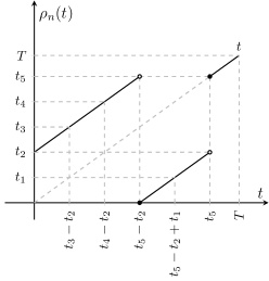
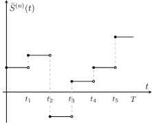
  Figure 2: Upper panel: representation of $\rho_{n}$ in $[0,T)$. Lower panel: sample path of $\bar{S}^{(n)}$ in $[0,T)$ (left) and the nondecreasing composition $\bar{S}^{(n)}\circ\rho_{n}$ (right).

• Since $\hat{\omega}^{(n)}\longrightarrow Z^{(\beta)}$ in $(\mathcal{D},J_{1})$ for any $\gamma_{1}\in\Omega^{\prime}_{1}$, we can apply [W1, Theorem 3.1], which gives sufficient conditions for the composition of two càdlàg functions to be continuous in the $J_{1}$ topology. Using (71)-(72) we will get

  $$\hat{\omega}^{(n)}\circ\bar{S}^{(n)}\circ\rho_{n}\longrightarrow Z^{(\beta)}\circ\mu\hskip 1.00006pt\mathrm{id}\qquad\text{in }(\mathcal{D}([0,T)),J_{1}),$$ (73)

  for any $(\gamma_{1},\gamma_{2})\in\Omega^{\prime}_{1}\times\,B_{\eta}$. By definition of $J_{1}$-convergence, there exists a sequence of homeomorphisms $\lambda_{n}$ of $[0,T)$, such that, as $n\to\infty$,

  $$\sup_{t\in[0,T)}|\lambda_{n}(t)-t|\to 0,$$ (74)

  $$\sup_{t\in[0,T)}|\hat{\omega}^{(n)}\circ\bar{S}^{(n)}\circ\rho_{n}\circ\lambda_{n}(t)-Z^{(\beta)}(\mu t)|\to 0.$$ (75)

• Note that (75) is exactly (68) for the bijection $\tau_{n}:=\rho_{n}\circ\lambda_{n}$. Therefore, it will remain to establish (69), that is,

  $$\sup_{t\in[0,T)}|\rho_{n}\circ\lambda_{n}(t)-t|\to 0.$$ (76)

We now fill the gaps in the steps above.

Construction of $\rho_{n}$.

We begin by constructing the bijection $\rho_{n}:[0,T)\longrightarrow[0,T)$. Since $\bar{S}^{(n)}(t)=S_{\lfloor nt\rfloor}/n$ for $t\in[0,T)$ and $\gamma_{2}\in B_{\eta}$, we have that

$$|S_{\lfloor u\rfloor}-\mu u|\leq C_{\eta}\hskip 1.00006ptn^{1/\alpha},$$ (77)

uniformly for $u\in[0,nT)$. Without loss of generality, we assume that $nT\in\mathbb{N}$. If not, one can take $T^{\prime}$ slightly larger than $T$, with $nT^{\prime}\in\mathbb{N}$, and work in $[0,T^{\prime}]$. Let $p(\cdot)$ be a permutation of $\{0,1,\dots,nT-1\}$ such that $S_{p(0)}\leq S_{p(1)}\leq\dots\leq\,S_{p(nT-1)}$. We define $\rho_{n}$ as follows:

$$\rho_{n}(t):=t-\frac{i}{n}+\frac{p(i)}{n},\qquad t\in\Big{[}\frac{i}{n},\frac{i+1}{n}\Big{)},\leavevmode\nobreak\ i\in\{0,\ldots,nT-1\}.$$ (78)

Clearly, $\rho_{n}$ is a bijection that maps $[i/n,(i+1)/n)$ affinely onto $[p(i)/n,(p(i)+1)/n)$. By construction of $p(\cdot)$, $\bar{S}^{(n)}\circ\rho_{n}$ is nondecreasing. The next proposition shows that $\rho_{n}$ is uniformly close to the identity.

Proposition 3.1.

For all $\gamma_{2}\in B_{\eta}$,

$$\sup_{i\in\{0,\ldots,nT-1\}}|i-p(i)|\leq\frac{2C_{\eta}}{\mu}\hskip 1.00006ptn^{1/\alpha}+1.$$ (79)

Proof.

To better explain the proof we refer to Figure 3, which shows a sample path of $u\mapsto S_{\lfloor u\rfloor}$ and the corresponding upper and lower bounds given by (77).

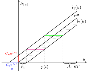
Figure 3: A sample path of $S_{\lfloor u\rfloor}$ and the corresponding upper and lower bounds given by (77) and represented by the graphs of the functions $l_{1}(u)=\mu u+C_{\eta}n^{1/\alpha}$ and $l_{2}(u)=\mu u-C_{\eta}n^{1/\alpha}$. The horizontal and verticals sizes of the strip are, respectively, $2C_{\eta}n^{1/\alpha}/\mu$ and $2C_{\eta}n^{1/\alpha}$. The sets $\mathcal{B}_{i},\mathcal{A}_{i}$ are defined in the body of the text.

We establish (79) by estimating from below the cardinality of the sets

$$L_{i}:=\{j\in\{0,\ldots,nT-1\}:S_{p(i)}\geq S_{j}\},$$ (80)

$$U_{i}:=\{j\in\{0,\ldots,nT-1\}:S_{p(i)}\leq S_{j}\}.$$ (81)

Let us begin with a lower bound for $|L_{i}|$. To this end, consider the interval $\mathcal{B}_{i}:=[0,b_{i,n}]\subseteq[0,nT)$, where $b_{i,n}:=p(i)-2C_{\eta}n^{1/\alpha}/\mu$. This set was introduced because it has the property that, for all $u\in\mathcal{B}_{i}$, $S_{\lfloor u\rfloor}\leq S_{p(i)}$, see Figure 3. Observe that, for small values of $p(i)$, $\mathcal{B}_{i}$ might be empty. These considerations show that

$$|L_{i}|\geq|\mathcal{B}_{i}\cap L_{i}|=|\mathcal{B}_{i}\cap\mathbb{Z}|=\max\{\lfloor b_{i,n}\rfloor+1,0\}.$$ (82)

On the other hand, since $S_{p(i)}$ is the $(i+1)$-th smallest value of the set $\{S_{j}\}_{j=0}^{nT-1}$, we know that $|L_{i}|=i+1$. From the above inequality, then,

$$i\geq\lfloor b_{i,n}\rfloor=\Big{\lfloor}p(i)-2\frac{C_{\eta}n^{1/\alpha}}{\mu}\Big{\rfloor}\geq p(i)-2\frac{C_{\eta}n^{1/\alpha}}{\mu}-1.$$ (83)

We proceed analogously to produce a lower bound for $|U_{i}|$. Set $\mathcal{A}_{i}:=[a_{i,n},nT)$, where $a_{i,n}=p(i)+2C_{\eta}n^{1/\alpha}/\mu$. Figure 3 shows that $S_{\lfloor t\rfloor}\geq S_{p(i)}$ for all $t\in\mathcal{A}_{i}$, whence $|\mathcal{A}_{i}\cap U_{i}|=\lfloor nT-a_{i,n}\rfloor+1$. On the other hand, $|U_{i}|=nT-i+1$. Since $|U_{i}|\geq|\mathcal{A}_{i}\cap U_{i}|$ we get

$$nT-i\geq\lfloor nT-a_{i,n}\rfloor\geq nT-a_{i,n}-1,$$ (84)

and so

$$i\leq a_{i,n}+1=p(i)+2\frac{C_{\eta}n^{1/\alpha}}{\mu}+1,$$ (85)

concluding the proof. ∎

$J_{2}$-convergence on $\Omega^{\prime}_{1}\times\,B_{\eta}$.

To derive (73) we first notice that, for any $\gamma_{2}\in B_{\eta}$,

$$\bar{S}^{(n)}\circ\rho_{n}\to\mu\hskip 1.00006pt\mathrm{id}\qquad\text{in }(\mathcal{D}([0,T)),J_{1}),$$ (86)

as $n\to\infty$. This is in fact a consequence of the following uniform convergence:

$$\begin{split}&\sup_{t\in[0,T)}|\bar{S}^{(n)}\circ\rho_{n}(t)-\mu\hskip 1.00006ptt|\\ &\qquad=\sup_{i\in\{0,\ldots,nT-1\}}\sup_{t\in[i/n,(i+1)/n)}\Big{|}\bar{S}^{(n)}\Big{(}t-\frac{i-p(i)}{n}\Big{)}-\mu\hskip 1.00006ptt\Big{|}\\ &\qquad\leq\sup_{i\in\{0,\ldots,nT-1\}}\sup_{t\in[i/n,(i+1)/n)}\Big{|}\bar{S}^{(n)}\Big{(}t-\frac{i-p(i)}{n}\Big{)}-\mu\Big{(}t-\frac{i-p(i)}{n}\Big{)}\Big{|}\\ &\qquad\quad+\sup_{i\in\{0,\ldots,nT-1\}}\Big{|}\frac{i-p(i)}{n}\Big{|}\\ &\qquad=C_{\eta}\frac{n^{1/\alpha}}{n}+\frac{2C_{\eta}}{\mu}\frac{n^{1/\alpha}}{n}+\frac{1}{n},\end{split}$$ (87)

which vanishes for $n\to\infty$. Now the plan is to once again apply [W1, Theorem 3.1] to show that (86) and the limit $\hat{\omega}^{(n)}\to Z^{(\beta)}$ in $(\mathcal{D},J_{1})$, which holds because $\gamma_{1}\in\Omega_{1}^{\prime}$, imply (73).

There is a problem, however. The theorem cannot be applied tout court because neither $\hat{\omega}^{(n)}$ nor $Z^{(\beta)}$ are càdlàg functions, cf (14)-(15). On the other hand, we can use the considerations of Remark 2.1 to show that $\hat{\omega}^{(n)}_{\mathrm{cadlag}}\to Z^{(\beta)}_{\mathrm{cadlag}}$ in $(\mathcal{D},J_{1})$ and thus, by [W1, Theorem 3.1],

$$\hat{\omega}^{(n)}_{\mathrm{cadlag}}\circ\bar{S}^{(n)}\circ\rho_{n}\longrightarrow Z^{(\beta)}_{\mathrm{cadlag}}\circ\mu\hskip 1.00006pt\mathrm{id}\qquad\text{in }(\mathcal{D}([0,T)),J_{1}).$$ (88)

But the restrictions of $Z^{(\beta)}_{\mathrm{cadlag}}$ and $Z^{(\beta)}$ to $[0,\mu T)$ coincide, so will obtain (73) when we prove that $\hat{\omega}^{(n)}_{\mathrm{cadlag}}\circ\bar{S}^{(n)}\circ\rho_{n}$ is asymptotic to $\hat{\omega}^{(n)}\circ\bar{S}^{(n)}\circ\rho_{n}$ in $(\mathcal{D}([0,T)),J_{1})$, as $n\to\infty$. We will show more, namely that, for some $C>0$,

$$\sup_{t\in\mathbb{R}^{+}}\left|\hat{\omega}^{(n)}_{\mathrm{cadlag}}\circ\bar{S}^{(n)}\circ\rho_{n}(t)-\hat{\omega}^{(n)}\circ\bar{S}^{(n)}\circ\rho_{n}(t)\right|\leq\frac{C}{n^{1/\beta}}.$$ (89)

In fact, with the help of (4) and (14) observe that

$$\hat{\omega}^{(n)}_{\mathrm{cadlag}}(s)-\hat{\omega}^{(n)}(s)=\left\{\begin{array}[]{ll}\displaystyle\frac{\zeta_{j}}{n^{1/\beta}}&\mbox{if }s=\displaystyle\frac{j}{n},\,j\in\mathbb{Z}^{-}\\[10.0pt] 0&\mbox{otherwise}\end{array}\right.\,,$$ (90)

where the numbers $\zeta_{j}$, for $j\in\mathbb{Z}^{-}$, are fixed, as the realization $\gamma_{1}\in\Omega_{1}^{\prime}$ of the medium is fixed. Now, the realization $\gamma_{2}\in B_{\eta}$ of the underlying random walk is also fixed. Since the drift $\mu$ is positive, $S_{n}<0$ occurs only for a finite number of times $n$. The values of these excursions below zero and their times are contained in this chain of inequalities $S_{p(0)}\leq S_{p(1)}\leq\ldots\leq S_{p(m-1)}<0\leq S_{p(m)}$, for some $m\in\mathbb{N}$. Thus

$$\sup_{t\in[0,p(m)/n)}\left|\hat{\omega}^{(n)}_{\mathrm{cadlag}}\circ\bar{S}^{(n)}\circ\rho_{n}(t)-\hat{\omega}^{(n)}\circ\bar{S}^{(n)}\circ\rho_{n}(t)\right|\leq\frac{\max\{\zeta_{j}\}_{j=S_{p(0)}}^{-1}}{n^{1/\beta}}.$$ (91)

Since the expression on the above l.h.s. is identically 0 for $t\geq p(m)/n$, we have proved (89), thus (73), thus (74)-(75).

We are left to prove that $\tau_{n}=\rho_{n}\circ\lambda_{n}$ satisfies (76). We do so with the help of Proposition 3.1:

$$\begin{split}\sup_{t\in[0,T)}|\rho_{n}\circ\lambda_{n}(t)-t|&=\sup_{s\in[0,T)}|\rho_{n}(s)-\lambda_{n}^{-1}(s)|\\ &=\sup_{i\in\{0,\ldots,nT-1\}}\sup_{s\in[i/n,(i+1)/n)}\Big{|}s-\frac{i-p(i)}{n}-\lambda_{n}^{-1}(s)\Big{|}\\ &\leq\sup_{s\in[0,T)}|s-\lambda_{n}^{-1}(s)|+\sup_{i\in\{0,\ldots,nT-1\}}\Big{|}\frac{p(i)-i}{n}\Big{|},\end{split}$$ (92)

which converges to 0 as $n\to\infty$ by (74) and (79). This finally shows that $\hat{\omega}^{(n)}\circ\bar{S}^{(n)}\to Z^{(\beta)}\circ\mu\hskip 1.00006pt\mathrm{id}$ in $(\mathcal{D}([0,T)),J_{2})$ for all $(\gamma_{1},\gamma_{2})\in\Omega^{\prime}_{1}\times B_{\eta}$, concluding the proof of Theorem 2.2.

3.4 Proof of Theorem 2.4: Limit theorems for the fluctuations

Once again, we only prove the theorem in the case $\mu>0$. Using definitions (19) and (25) we write

$$n(\bar{Y}^{(n)}-\mu\nu\hskip 1.00006pt\mathrm{id})=n^{1/\beta}\tilde{\omega}^{(n)}\circ\bar{S}^{(n)}+n^{1/\alpha}\nu\tilde{S}^{(n)}+\nu\mu(\lfloor n\hskip 1.00006pt\mathrm{id}\rfloor-n\hskip 1.00006pt\mathrm{id}).$$ (93)

The asymptotic behavior of (93) depends crucially on the ratio $\alpha/\beta$, hence we distinguish three cases. Observe that since $(\lfloor n\hskip 1.00006pt\mathrm{id}\rfloor-n\hskip 1.00006pt\mathrm{id})$ is bounded, the last term of the above r.h.s. vanishes in the limit, whether we divide it by $n^{1/\alpha}$ or by $n^{1/\beta}$.

Case $\alpha<\beta$.

Substituting $\hat{\omega}^{(n)}$ with $\tilde{\omega}^{(n)}$ and $Z^{(\beta)}$ with $\tilde{Z}^{(\beta)}$, cf. (20), in the proof of Theorem 2.2, one shows that, for $\beta\in(1,2)$ and $n\to\infty$,

$$\tilde{\omega}^{(n)}\circ\bar{S}^{(n)}\xrightarrow{\>\>\text{d}\>\>}\mu^{1/\beta}\tilde{Z}_{+}^{(\beta)}\IfEqCase{2}{{1}{\qquad\text{in }(\mathcal{D}^{+},J_{1})}{2}{\qquad\text{in }(\mathcal{D}^{+},J_{2})}}[].$$ (94)

Since in this case $1/\alpha>1/\beta$, we obtain

$$\frac{\tilde{\omega}^{(n)}\circ\bar{S}^{(n)}}{n^{1/\alpha-1/\beta}}\xrightarrow{\>\>\text{d}\>\>}0\IfEqCase{1}{{1}{\qquad\text{in }(\mathcal{D}^{+},J_{1})}{2}{\qquad\text{in }(\mathcal{D}^{+},J_{2})}}[],$$ (95)

where we have observed that we can pass from $J_{2}$-convergence to $J_{1}$-convergence because both convergences reduce to uniform convergence when the limit function is continuous, cf. Remark 2.3. Finally, by (93), (95) and (26),

$$\frac{n(\bar{Y}^{(n)}-\mu\nu\hskip 1.00006pt\mathrm{id})}{n^{1/\alpha}}\xrightarrow{\>\>\text{d}\>\>}\nu\widetilde{W}^{(\alpha)}\qquad\text{in }(\mathcal{D}^{+},J_{1}),$$ (96)

which amounts to (36), as desired.

Case $\alpha>\beta$.

Since in this case $1/\beta>1/\alpha$, the leading order term in (93) is the first term, whose limit has been identified in (94). We conclude that

$$\frac{n(\bar{Y}^{(n)}-\mu\nu\hskip 1.00006pt\mathrm{id})}{n^{1/\beta}}\xrightarrow{\>\>\text{d}\>\>}\mu^{1/\beta}\,\tilde{Z}_{+}^{(\beta)}\IfEqCase{2}{{1}{\qquad\text{in }(\mathcal{D}^{+},J_{1})}{2}{\qquad\text{in }(\mathcal{D}^{+},J_{2})}}[],$$ (97)

i.e., (38) holds for the case $\mu>0$.

Case $\alpha=\beta$.

Except for certain complications, the proof of this case will follow the same ideas as that of Theorem 2.2 in Section 3.3. We will detail the parts that need a new argument and describe quickly those that are proved exactly as done earlier.

In view of (93), we rewrite our process of interest as

$$\tilde{Y}^{(n)}=\tilde{\omega}^{(n)}\circ\bar{S}^{(n)}+\nu\tilde{S}^{(n)}+\delta_{n}=\ell\big{(}h\big{(}\tilde{\omega}^{(n)},\bar{S}^{(n)}\big{)},\nu\tilde{S}^{(n)}\big{)}+\delta_{n},$$ (98)

where $h(x,y):=x\circ y$ is the composition map from $\mathcal{D}\times\mathcal{D}^{+}$ to $\mathcal{D}^{+}$ and $\ell(x,y):=x+y$ is the addition map from $\mathcal{D}^{+}\times\mathcal{D}^{+}$ to $\mathcal{D}^{+}$. Also $\delta_{n}:=\nu\mu(\lfloor n\hskip 1.00006pt\mathrm{id}\rfloor-n\hskip 1.00006pt\mathrm{id})/n^{1/\alpha}$ is a negligible term, as $n\to\infty$, in any relevant distance. As was done in Section 3.3, we use the Skorokhod Representation Theorem twice to obtain two probability spaces $(\Omega_{1},\mathbb{P}_{1})$ and $(\Omega_{2},\mathbb{P}_{2})$, and processes

$$\begin{array}[]{l}\boldsymbol{\tilde{\omega}^{(n)}}:\Omega_{1}\to\mathcal{D},\\ \boldsymbol{\tilde{Z}^{(\alpha)}}:\Omega_{1}\to\mathcal{D},\\ \boldsymbol{\bar{S}^{(n)}}:\Omega_{2}\to\,\mathcal{D}^{+},\\ \boldsymbol{\tilde{S}^{(n)}}:\Omega_{2}\to\,\mathcal{D}^{+},\\ \boldsymbol{\widetilde{W}^{(\alpha)}}:\Omega_{2}\to\mathcal{D}^{+},\end{array}$$ (99)

with respectively the same distribution as $\tilde{\omega}^{(n)},\tilde{Z}^{(\alpha)},\bar{S}^{(n)},\tilde{S}^{(n)}$ and $\widetilde{W}^{(\alpha)}$, and such that

$$\begin{array}[]{lll}\boldsymbol{\tilde{\omega}}^{(n)}\xrightarrow{\>\>\text{a.s.}\>\>}\boldsymbol{\tilde{Z}^{(\alpha)}}&\text{on }(\Omega_{1},\mathbb{P}_{1})&\IfEqCase{1}{{1}{\qquad\text{in }(\mathcal{D},J_{1})}{2}{\qquad\text{in }(\mathcal{D},J_{2})}}[]\\ \boldsymbol{\bar{S}^{(n)}}\xrightarrow{\>\>\text{a.s.}\>\>}\mu\hskip 1.00006pt\mathrm{id}&\text{on }(\Omega_{2},\mathbb{P}_{2})&\IfEqCase{1}{{1}{\qquad\text{in }(\mathcal{D}^{+},J_{1})}{2}{\qquad\text{in }(\mathcal{D}^{+},J_{2})}}[]\\ \boldsymbol{\tilde{S}^{(n)}}\xrightarrow{\>\>\text{a.s.}\>\>}\boldsymbol{\widetilde{W}^{(\alpha)}}&\text{on }(\Omega_{2},\mathbb{P}_{2})&\IfEqCase{1}{{1}{\qquad\text{in }(\mathcal{D}^{+},J_{1})}{2}{\qquad\text{in }(\mathcal{D}^{+},J_{2})}}[]\end{array}\,$$ (100)

Once again, since the processes relative to the medium and those relative to the dynamics are independent, it is correct to regard all boldface processes as defined on $(\Omega_{1}\times\Omega_{2},\mathbb{P}_{1}\times\mathbb{P}_{2})$. Again we simplify the notation and use the regular typeset for all processes (99). Let us define

$$\Omega_{1}^{\prime} :=\{\gamma_{1}\in\Omega_{1}\,:\,\tilde{\omega}^{(n)}{[\gamma_{1}]}\to\tilde{Z}^{(\alpha)}[\gamma_{1}]\mbox{ in }(\mathcal{D},J_{1})\},$$ (101)

$$\Omega_{2}^{\prime} :=\{\gamma_{2}\in\Omega_{2}\,:\,\tilde{S}^{(n)}{[\gamma_{2}]}\to\widetilde{W}^{(\alpha)}[\gamma_{2}]\mbox{ in }(\mathcal{D}^{+},J_{1})\}.$$ (102)

These are full-measure sets in their respective spaces. Notice that (essentially by the definition of $\tilde{S}^{(n)}$) $\bar{S}^{(n)}{[\gamma_{2}]}\to\mu\hskip 1.00006pt\mathrm{id}$, for all $\gamma_{2}\in\Omega_{2}^{\prime}$. Now let us fix $T>0$. We already know that for any $\eta\in(0,1)$, there exist $C_{\eta}>0$ and $\bar{n}_{\eta}\in\mathbb{N}$ (both numbers depending on $T$ as well) such that the set

$$B_{\eta}:=\Big{\{}\gamma_{2}\in\Omega^{\prime}_{2}:\sup_{t\in[0,T)}\frac{n|\bar{S}^{(n)}{[\gamma_{2}]}(t)-\mu\hskip 1.00006ptt|}{n^{1/\alpha}}\leq C_{\eta}\text{ for }n\geq\bar{n}_{\eta}\Big{\}}$$ (103)

has measure $\mathbb{P}_{2}(B_{\eta})>1-\eta$. Now one proceeds as in the proof of Theorem 2.2, using $\tilde{\omega}^{(n)}$ and $\tilde{Z}^{(\alpha)}$ in place of $\hat{\omega}^{(n)}$ and $Z^{(\beta)}$, respectively. The fact that now $\beta=\alpha\in(1,2)$ causes no breaks in the proof. One obtains that, for all $(\gamma_{1},\gamma_{2})\in\Omega^{\prime}_{1}\times B_{\eta}$,

$$h(\tilde{\omega}^{(n)},\bar{S}^{(n)})=\tilde{\omega}^{(n)}\circ\bar{S}^{(n)}\to\tilde{Z}^{(\alpha)}\circ\mu\hskip 1.00006pt\mathrm{id}\qquad\text{in }(\mathcal{D}([0,T)),J_{2}).$$ (104)

By construction of $B_{\eta}$, $\nu\tilde{S}^{(n)}\to\nu\widetilde{W}^{(\alpha)}$ in $(\mathcal{D}([0,T)),J_{2})$ for all $\gamma_{2}\in B_{\eta}$. If we are able to prove that, for all $(\gamma_{1},\gamma_{2})\in\Omega^{\prime}_{1}\times B_{\eta}$, the addition map $\ell$ is continuous at $(\tilde{Z}^{(\alpha)}\circ\mu\hskip 1.00006pt\mathrm{id},\,\nu\widetilde{W}^{(\alpha)})$ in the space $\mathcal{D}([0,T)),J_{2})$, we obtain by (98) that

$$\lim_{n\to\infty}\tilde{Y}^{(n)}=\lim_{n\to\infty}\ell\big{(}h\big{(}\tilde{\omega}^{(n)},\bar{S}^{(n)}\big{)},\nu\tilde{S}^{(n)}\big{)}=\tilde{Z}^{(\alpha)}\circ\mu\hskip 1.00006pt\mathrm{id}+\nu\widetilde{W}^{(\alpha)},$$ (105)

for all realizations $(\gamma_{1},\gamma_{2})\in\Omega^{\prime}_{1}\times B_{\eta}$. Since $\eta\in(0,1)$ is arbitrary, the above limit extends to an almost sure limit in $(\Omega_{1}\times\Omega_{2},\mathbb{P}_{1}\times\mathbb{P}_{2})$. Passing to distributional convergence and (freely) varying the choice of $T$, we finally achieve (40) for the case $\mu>0$. This ends the proof of Theorem 2.4.

It remains to show that the addition map on $(\mathcal{D}([0,T)),J_{2})$ is continuous under standard conditions. For a general space of càdlàg functions, Whitt proves that $\ell$ is continuous, relative to the topologies $J_{1}$, $M_{1}$ or $M_{2}$, at all pairs $(x,y)$ such that $\text{Disc}(x)\cap\text{Disc}(y)=\emptyset$ (see [W1, Theorem 4.1] and [W2, Corollaries 12.7.1 & 12.11.5], respectively). In Theorem A.1 of the Appendix we extend this statement to the topology $J_{2}$. As for its applicability to our case, notice that we can indeed assume that, for all $(\gamma_{1},\gamma_{2})\in\Omega^{\prime}_{1}\times B_{\eta}$,

$$\text{Disc}(\widetilde{Z}^{(\alpha)}\circ\mu\hskip 1.00006pt\mathrm{id})\cap\text{Disc}(\nu\tilde{W}^{(\alpha)})=\emptyset,$$ (106)

because $\widetilde{Z}^{(\alpha)}$ and $\tilde{W}^{(\alpha)}$ are independent $\alpha$-stable processes and one can always remove from $\Omega_{1}^{\prime}\times\Omega_{2}^{\prime}$ the null set of realizations for which (106) does not hold.

Appendix A Appendix: Continuity of the addition map in $J_{2}$

Theorem A.1.

Let $I$ be a (closed, open or half-open) bounded interval. The addition map $\ell:\mathcal{D}(I)\times\mathcal{D}(I)\longrightarrow\mathcal{D}(I)$ defined by $\ell(x,y):=x+y$ is measurable and it is $J_{2}$-continuous at all pairs $(x,y)$ such that

$$\mathrm{Disc}(x)\cap\mathrm{Disc}(y)=\emptyset.$$ (107)

The latter assertion amounts to the claim that $d_{J_{2},I}(x_{n},x)\to 0$ and $d_{J_{2},I}(y_{n},y)\to 0$, as $n\to\infty$, imply $d_{J_{2},I}(x_{n}+y_{n},x+y)\to 0$.

Proof.

We follow the same line of arguments as in the proof of [W1, Theorem 4.1]. In fact, the measurability of $\ell$ is proved exactly as in the referenced theorem. As for the continuity claim, we fix $I:=[a,b)$, which is the case needed in Section 3.4. The other three cases, $I=[a,b]$, $I=(a,b]$ or $I=(a,b)$, are proved exactly in the same way. Without loss of generality, we also assume to work with càdlàg functions (as opposed to functions that have a càdlàg and a càglàd restriction). This case happens, e.g., if $0\leq a<b$.

For a fixed $\varepsilon>0$, we must show that there exist $\bar{n}\in\mathbb{Z}^{+}$ and, for all $n\geq\bar{n}$, bijections ${\lambda}_{n}:[a,b)\longrightarrow[a,b)$ such that

$$\sup_{t\in[a,b)}|{\lambda}_{n}(t)-t| <\varepsilon,$$ (108)

$$\sup_{t\in[a,b)}|(x_{n}+y_{n})\circ{\lambda}_{n}(t)-(x+y)(t)| <\varepsilon.$$ (109)

Since $x,y$ are càdlàg, by [B, Chapter 3, Lemma 1] there exist two finite sets of points

$$\mathcal{P}_{x} =\{a=t_{0},t_{1},...,t_{n},t_{n+1}=b\}$$ (110)

$$\mathcal{P}_{y} =\{a=s_{0},s_{1},...,s_{m},s_{m+1}=b\}$$ (111)

such that, for all $i=1,\ldots,n+1$ and $j=1,\ldots,m+1$,

$$\sup_{q_{1},q_{2}\in[t_{i-1},t_{i})}|x(q_{1})-x(q_{2})|<\frac{\varepsilon}{8},$$ (112)

$$\sup_{q_{1},q_{2}\in[s_{i-1},s_{i})}|y(q_{1})-y(q_{2})|<\frac{\varepsilon}{8}.$$ (113)

From this construction we have that the discontinuity points of $x$ (respectively $y$) with jump size bigger than $\varepsilon/8$ are contained in $\mathcal{P}_{x}$ (respectively $\mathcal{P}_{y}$). By hypothesis these two sets of points are disjoint. Moreover, we can select the other points of $\mathcal{P}_{x}$ and $\mathcal{P}_{y}$ so that $\mathcal{P}_{x}\cap\mathcal{P}_{y}=\{a,b\}$. Let $4\delta$ be the distance between the closest pair of points of $\mathcal{P}:=\mathcal{P}_{x}\cup\mathcal{P}_{y}$. For $i=1,\ldots,n$ and $j=1,\ldots,m$, we construct closed intervals $\mathcal{J}_{i}^{(x)}$ and $\mathcal{J}_{j}^{(y)}$ such that

$$[t_{i}-\delta,t_{i}+\delta]\subset\mathrm{int}\big{(}\mathcal{J}_{i}^{(x)}\big{)} \subset\mathcal{J}_{j}^{(y)}\subset(t_{i}-2\delta,t_{i}+2\delta),$$ (114)

$$[s_{j}-\delta,s_{j}+\delta]\subset\mathrm{int}\big{(}\mathcal{J}_{i}^{(x)}\big{)} \subset\mathcal{J}_{j}^{(y)}\subset(s_{j}-2\delta,s_{j}+2\delta).$$ (115)

This implies in particular that these intervals are pairwise disjoint.

Now let us assume that there exist $\bar{n}\in\mathbb{Z}^{+}$ and bijections $\mu_{n},\nu_{n}:[a,b)\longrightarrow[a,b)$ so that, for all $n\geq\bar{n}$,

$$\sup_{t\in[a,b)}|\mu_{n}(t)-t|<\min\{\varepsilon,\delta\},\quad\sup_{t\in[a,b)}|x_{n}\circ\mu_{n}(t)-x(t)| <\frac{\varepsilon}{4},\quad\mu_{n}(\mathcal{J}_{i}^{(x)})=\mathcal{J}_{i}^{(x)}$$ (116)

$$\sup_{t\in[a,b)}|\nu_{n}(t)-t|<\min\{\varepsilon,\delta\},\quad\sup_{t\in[a,b)}|y_{n}\circ\nu_{n}(t)-y(t)| <\frac{\varepsilon}{4},\quad\nu_{n}(\mathcal{J}_{j}^{(y)})=\mathcal{J}_{j}^{(y)}$$ (117)

for all $i=1,\ldots,n$ and $j=1,\ldots,m$. The first and second conditions in both (116) and (117) can be satisfied by the hypotheses $x_{n}\to x$, $y_{n}\to y$ in $(\mathcal{D}([a,b)),J_{2})$. We postpone for a moment the proof that $\mu_{n},\nu_{n}$ can be found to satisfy the third conditions as well. Let us construct the bijection ${\lambda}_{n}:[a,b)\longrightarrow[a,b)$ as follows:

$${\lambda}_{n}(t):=\begin{cases}\mu_{n}(t)&\mbox{ for }t\in\mathcal{J}_{i}^{(x)}\mbox{ with }i=1,\ldots,n,\\ \nu_{n}(t)&\mbox{ for }t\in\mathcal{J}_{j}^{(y)}\mbox{ with }j=1,\ldots,m,\\ t&\mbox{ otherwise}.\end{cases}$$ (118)

We have the following estimates:

$$\sup_{t\in\mathcal{J}_{i}^{(x)}}|x_{n}\circ{\lambda}_{n}(t)-x(t)|=\sup_{t\in\mathcal{J}_{i}^{(x)}}|x_{n}\circ\mu_{n}(t)-x(t)|<\frac{\varepsilon}{4},$$ (119)

by (116), and

$$\begin{split}&\sup_{t\in\mathcal{J}_{j}^{(y)}}|x_{n}\circ{\lambda}_{n}(t)-x(t)|\\ &\qquad=\sup_{t\in\mathcal{J}_{j}^{(y)}}|x_{n}\circ\nu_{n}(t)-x(t)|\\ &\qquad\leq\sup_{t\in\mathcal{J}_{j}^{(y)}}|x_{n}\circ\nu_{n}(t)-x\circ\mu_{n}^{-1}\circ\nu_{n}(t)|+\sup_{t\in\mathcal{J}_{j}^{(y)}}|x\circ\mu_{n}^{-1}\circ\nu_{n}(t)-x(t)|\\ &\qquad\leq\sup_{u\in[a,b)}|x_{n}\circ\mu_{n}(u)-x(u)|+\sup_{t\in\mathcal{J}_{j}^{(y)}}|x(\mu_{n}^{-1}\circ\nu_{n}(t))-x(t)|\\ &\qquad<\frac{\varepsilon}{4}+\frac{\varepsilon}{8}=\frac{3\varepsilon}{8}.\end{split}$$ (120)

In the first term of the final estimate of (120) we have renamed $u:=\mu_{n}^{-1}\circ\nu_{n}(t)$ and used (116). For the second term we have observed that, by (116)-(117), the bijection $\mu_{n}^{-1}\circ\nu_{n}$ is closer to the identity than $2\delta$. Since $t\in\mathcal{J}_{j}^{(y)}$ this implies, by (115), that $t$ and $\mu_{n}^{-1}\circ\nu_{n}(t)$ belong to the same interval $[t_{i-1},t_{i})$, for some $i$. Thus we have used (112). Lastly, if we denote $\mathcal{J}:=\big{(}\bigsqcup_{i=1}^{n}\mathcal{J}_{i}^{(x)}\big{)}\sqcup\big{(}\bigsqcup_{j=1}^{m}\mathcal{J}_{j}^{(y)}\big{)}$,

$$\begin{split}&\sup_{t\in[a,b)\setminus\mathcal{J}}|x_{n}\circ{\lambda}_{n}(t)-x(t)|\\ &\qquad=\sup_{t\in[a,b)\setminus\mathcal{J}}|x_{n}(t)-x(t)|\\ &\qquad\leq\sup_{t\in[a,b)\setminus\mathcal{J}}|x_{n}(t)-x\circ\mu_{n}^{-1}(t)|+\sup_{t\in[a,b)\setminus\mathcal{J}}|x\circ\mu_{n}^{-1}(t)-x(t)|\\ &\qquad\leq\sup_{u\in[a,b)}|x_{n}\circ\mu_{n}(u)-x(u)|+\sup_{t\in[a,b)\setminus\mathcal{J}}|x(\mu_{n}^{-1}(t))-x(t)|\\ &\qquad<\frac{\varepsilon}{4}+\frac{\varepsilon}{8}=\frac{3\varepsilon}{8},\end{split}$$ (121)

where we have used the same arguments as for (120): observe in fact that if $t\not\in\mathcal{J}$ then, by (114)-(115), $t$ is at distance larger than $\delta$ from $\mathcal{P}\setminus\{a,b\}$. By (116) $|\mu_{n}^{-1}(t)-t|<\delta$ and so $t$ and $\mu_{n}^{-1}(t)$ belong to the same interval $[t_{i-1},t_{i})$, for some $i$, triggering (112).

From (119)-(121) we have that $\sup_{t\in[a,b)}|x_{n}\circ{\lambda}_{n}(t)-x(t)|<\varepsilon/2$, and the same obviously holds for $y$, whence

$$\begin{split}&\sup_{t\in[a,b)}|(x_{n}+y_{n})\circ{\lambda}_{n}(t)-(x+y)(t)|\\ &\qquad\leq\sup_{t\in[a,b)}|x_{n}\circ{\lambda}_{n}(t)-x(t)|+\sup_{t\in[a,b)}|y_{n}\circ{\lambda}_{n}(t)-y(t)|<\varepsilon,\end{split}$$ (122)

giving (109). The inequality (108) follows from definition (118) and (116)-(117) and so Theorem A.1 is proved.

It remains to show that the bijections $\mu_{n},\nu_{n}$ can be chosen to satisfy the rightmost conditions of (116)-(117), for a suitable choice of the intervals $\{\mathcal{J}_{i}^{(x)}\}_{i=1}^{n}$, $\{\mathcal{J}_{j}^{(y)}\}_{j=1}^{m}$. We proceed by explicitly constructing $\mu_{n}$, as the construction of $\nu_{n}$ is completely analogous.

The hypothesis $d_{J_{2},[a,b)}(x_{n},x)\to 0$ amounts to the existence of bijections $\rho_{n}:[a,b)\longrightarrow[a,b)$ such that, for $n\geq\bar{n}$,

$$\sup_{t\in[a,b)}|\rho_{n}(t)-t| <\frac{1}{2}\min\{\varepsilon,\delta\},$$ (123)

$$\sup_{t\in[a,b)}|x_{n}\circ\rho_{n}(t)-x(t)| <\frac{\varepsilon}{8}.$$ (124)

For $i=1,\ldots,n$, set $[a_{i},b_{i}]:=[t_{i}-\delta,t_{i}+\delta]$ and

$$\mathcal{J}_{i}^{(x)}:=[a_{i}^{\prime\prime},b_{i}^{\prime\prime}]:=\left[\inf\!\big{(}\{a_{i}\}\cup\rho_{n}([a_{i},b_{i}])\big{)}-\frac{\delta}{2}\,,\,\sup\!\big{(}\{b_{i}\}\cup\rho_{n}([a_{i},b_{i}])\big{)}+\frac{\delta}{2}\right].$$ (125)

By construction $|a_{i}^{\prime\prime}-t_{i}|<2\delta$ and $|b_{i}^{\prime\prime}-t_{i}|<2\delta$. Hence the intervals $\mathcal{J}_{i}^{(x)}$ satisfy (114).

The bijection $\mu_{n}:[a,b)\longrightarrow[a,b)$ is defined with the following structure:

$$\mu_{n}(t):=\begin{cases}\mu_{n}^{(i)}(t)&\mbox{ for }t\in\mathcal{J}_{i}^{(x)}\mbox{ with }i=1,\ldots,n,\\ t&\mbox{ otherwise},\end{cases}$$ (126)

where $\mu_{n}^{(i)}:\mathcal{J}_{i}^{(x)}\longrightarrow\mathcal{J}_{i}^{(x)}$ are bijections that we construct in several steps as follows.

First, on $[a_{i},b_{i}]\subset\mathcal{J}_{i}^{(x)}$, we define $\mu_{n}^{(i)}|_{[a_{i},b_{i}]}:=\rho_{n}|_{[a_{i},b_{i}]}$. In light of (125) and applying (123) to $t\in[a_{i},b_{i}]$, we see that

$$\mu_{n}^{(i)}([a_{i},b_{i}])=\rho_{n}([a_{i},b_{i}])\subset(a_{i}^{\prime\prime},b_{i}^{\prime\prime})\subset\mathcal{J}_{i}^{(x)}.$$ (127)

Denote $\mathcal{A}_{i}:=[a_{i}^{\prime\prime},t_{i})\setminus\mu_{n}^{(i)}([a_{i},b_{i}])$ and $\mathcal{B}_{i}:=[t_{i},b_{i}^{\prime\prime}]\setminus\mu_{n}^{(i)}([a_{i},b_{i}])$. These are, respectively, the lower and upper parts of $[a_{i}^{\prime\prime},b_{i}^{\prime\prime}]=\mathcal{J}_{i}^{(x)}$ that have not yet been assigned as image points of $\mu_{n}^{(i)}$ (which is only partially defined at this stage). Using the fact that the inequality (123) is strict, we can find $\eta$ with $0<\eta<\min\{\varepsilon,\delta\}/2$ such that

$$\inf\mu_{n}^{(i)}([a_{i},b_{i}])>a_{i}-\eta\,, \qquad\sup\mathcal{A}_{i}<a_{i}+\eta\,,$$ (128)

$$\sup\mu_{n}^{(i)}([a_{i},b_{i}])<b_{i}+\eta\,, \qquad\inf\mathcal{B}_{i}>b_{i}-\eta.$$ (129)

Set $a_{i}^{\prime}:=a_{i}-\eta$ and $b_{i}^{\prime}:=b_{i}+\eta$. We have $a_{i}^{\prime\prime}<a_{i}^{\prime}<a_{i}<b_{i}<b_{i}^{\prime}<b_{i}^{\prime\prime}$. The inequalities (128) show that the yet-to-be-assigned image set $\mathcal{A}_{i}$ can we written as

$$\mathcal{A}_{i}=[a_{i}^{\prime\prime},a_{i}^{\prime}]\sqcup(\mathcal{A}_{i}\cap(a_{i}^{\prime},a_{i}+\eta)),$$ (130)

where $\mathcal{A}_{i}\cap(a_{i}^{\prime},a_{i}+\eta)$ has the cardinality of the continuum because, by the first inequality of (128), there exists $\sigma>0$ such that $(a_{i}^{\prime},a_{i}^{\prime}+\sigma)\subset\mathcal{A}_{i}\cap(a_{i}^{\prime},a_{i}+\eta)$. By reasons of cardinality, then, there exists a bijection $\phi_{i}^{-}:(a_{i}^{\prime},a_{i})\longrightarrow\mathcal{A}_{i}\cap(a_{i}^{\prime},a_{i}+\eta)$. By construction, since $a_{i}^{\prime}=a_{i}-\eta$,

$$\sup_{t\in(a_{i}^{\prime},a_{i})}|\phi_{i}^{-}(t)-t|\leq 2\eta<\min\{\varepsilon,\delta\}.$$ (131)

We define $\mu_{n}^{(i)}|_{(a_{i}^{\prime},a_{i})}:=\phi_{i}^{-}$ and $\mu_{n}^{(i)}|_{[a_{i}^{\prime\prime},a_{i}^{\prime}]}:=\mathrm{id}$. Analogously, the inequalities (129) give

$$\mathcal{B}_{i}=(\mathcal{B}_{i}\cap(b_{i}-\eta,b_{i}^{\prime}))\sqcup[b_{i}^{\prime},b_{i}^{\prime\prime}]$$ (132)

and there exists a bijection $\phi_{i}^{+}:(b_{i},b_{i}^{\prime})\longrightarrow\mathcal{B}_{i}\cap(b_{i}-\eta,b_{i}^{\prime})$ for which the analogue of estimate (131) holds. Finally, we define $\mu_{n}^{(i)}|_{(b_{i},b_{i}^{\prime})}:=\phi_{i}^{+}$ and $\mu_{n}^{(i)}|_{[b_{i}^{\prime},b_{i}^{\prime\prime}]}:=\mathrm{id}$. This completes the definition of $\mu_{n}^{(i)}$ as a bijection of $\mathcal{J}_{i}^{(x)}$.

By (123), (131) and its analogue for $\phi_{i}^{+}$, we see that

$$\sup_{t\in\mathcal{J}_{i}^{(x)}}|\mu_{n}^{(i)}(t)-t|<\min\{\varepsilon,\delta\}.$$ (133)

Also, by the definition of $\mu_{n}^{(i)}|_{[a_{i},b_{i}]}$ and (124),

$$\sup_{t\in[a_{i},b_{i}]}|x_{n}\circ\mu_{n}^{(i)}(t)-x(t)|<\frac{\varepsilon}{8}.$$ (134)

Furthermore,

$$\sup_{t\in\mathcal{J}_{i}^{(x)}\setminus[a_{i},b_{i}]}|x_{n}\circ\mu_{n}^{(i)}(t)-x(t)|$$

$$\qquad\leq\sup_{t\in\mathcal{J}_{i}^{(x)}\setminus[a_{i},b_{i}]}\!|x_{n}\circ\mu_{n}^{(i)}(t)-x\circ\rho_{n}^{-1}\circ\mu_{n}^{(i)}(t)|+\!\sup_{t\in\mathcal{J}_{i}^{(x)}\setminus[a_{i},b_{i}]}\!|x\circ\rho_{n}^{-1}\circ\mu_{n}^{(i)}(t)-x(t)|$$

$$\qquad\leq\frac{\varepsilon}{8}+\frac{\varepsilon}{8}=\frac{\varepsilon}{4}.$$ (135)

The above estimates are derived in a way similar to that used in (120): for the first term we use (124) after the change of variable $u:=\rho_{n}^{-1}\circ\mu_{n}^{(i)}(t)$; for the second term we use (112) and the fact that $t$ and $\rho_{n}^{-1}\circ\mu_{n}^{(i)}(t)$ belong to the same interval $[t_{k-1},t_{k})$, for some $k$ (this is because, due to (123) and (133), $t\in\mathcal{J}_{i}^{(x)}$ and $|\rho_{n}^{-1}\circ\mu_{n}^{(i)}(t)-t|<3\delta/2$). Moreover, denoting $\mathcal{J}^{(x)}:=\bigsqcup_{i=1}^{n}\mathcal{J}_{i}^{(x)}$, it is now easy to use (124), (114) and (112) to estimate

$$\begin{split}&\sup_{t\in[a,b)\setminus\mathcal{J}^{(x)}}|x_{n}\circ\mu_{n}(t)-x(t)|\\ &\qquad=\sup_{t\in[a,b)\setminus\mathcal{J}^{(x)}}|x_{n}(t)-x(t)|\\ &\qquad\leq\sup_{t\in[a,b)\setminus\mathcal{J}^{(x)}}|x_{n}(t)-x\circ\rho_{n}^{-1}(t)|\>+\sup_{t\in[a,b)\setminus\mathcal{J}^{(x)}}|x\circ\rho_{n}^{-1}(t)-x(t)|\\[2.0pt] &\qquad<\frac{\varepsilon}{8}+\frac{\varepsilon}{8}=\frac{\varepsilon}{4}.\end{split}$$ (136)

Finally, the definition (126) of $\mu_{n}$ and the inequalities (133)-(136) yield (116) and conclude the proof of Theorem A.1. ∎

Remark A.1.

One can define a new topology of the Skorokhod type in the same way as Definitions 2.1 and 2.3 but taking the infimum in (7) over all piecewise increasing and continuous (PIC) bijections $\lambda:I\longrightarrow I$. A PIC bijection $\lambda:I\longrightarrow I$ is one such that $I$ can be partitioned into a finite number of intervals, on each of which $\lambda$ is increasing and continuous. Observe that in this case $\lambda^{-1}$ is also a PIC bijection. For want of a better name, let us call this topology $J_{3/2}$. Evidently, $J_{3/2}$ is weaker than $J_{1}$ and stronger than $J_{2}$. It is not hard to see that Theorem A.1 can be proved as well with the $J_{3/2}$-distance in place of the $J_{2}$-distance. Furthermore, in the proofs of Theorems 2.2 and 2.4, every time we needed to construct a sequence of bijections in order to prove a $J_{2}$-convergence, we have indeed produced a sequence of PIC bijections. Therefore, all assertions in this paper that are stated for the topology $J_{2}$, see (30), (38), (40), hold for the topology $J_{3/2}$ as well.

References

• [ACOR] R. Artuso, G. Cristadoro, M. Onofri, M. Radice, Non-homogeneous persistent random walks and Lévy-Lorentz gas, J. Stat. Mech. Theory Exp. 2018, no. 8, 083209, 13 pp.
• [BFK] E. Barkai, V. Fleurov, J. Klafter, One-dimensional stochastic Lévy-Lorentz gas, Phys. Rev. E 61 (2000), no. 2, 1164–1169.
• [BR] N. Berger, R. Rosenthal, Random walks on discrete point processes, Ann. Inst. Henri Poincaré Probab. Stat. 51 (2015), no. 2, 727–755.
• [BCLL] A. Bianchi, G. Cristadoro, M. Lenci, M. Ligabò, Random walks in a one-dimensional Lévy random environment, J. Stat. Phys. 163 (2016), no. 1, 22–40.
• [BLP] A. Bianchi, M. Lenci, F. Pène, Continuous-time random walk between Lévy-spaced targets in the real line, Stochastic Process. Appl. 130 (2020), no. 2, 708-732.
• [B] P. Billingsley, Convergence of probability measures, John Wiley & Sons, Inc., New York-London-Sydney, 1968.
• [BCV] R. Burioni, L. Caniparoli, A. Vezzani, Lévy walks and scaling in quenched disordered media, Phys. Rev. E 81 (2010), 060101(R), 4 pp.
• [BDLV] R. Burioni, S. di Santo, S. Lepri, A. Vezzani, Scattering lengths and universality in superdiffusive Lévy materials, Phys. Rev. E 86 (2012), 031125, 7 pp.
• [CF] P. Caputo, A. Faggionato, Diffusivity in one-dimensional generalized Mott variable-range hopping models, Ann. Appl. Probab. 19 (2009), no. 4, 1459–1494.
• [CFP] P. Caputo, A. Faggionato, T. Prescott, Invariance principle for Mott variable range hopping and other walks on point processes, Ann. Inst. Henri Poincaré Probab. Stat. 49 (2013), no. 3, 654–697.
• [CGLS] G. Cristadoro, T. Gilbert, M. Lenci, D. P. Sanders, Transport properties of Lévy walks: an analysis in terms of multistate processes, Europhys. Lett. 108 (2014), no. 5, 50002, 6 pp.
• [EK] S. N. Ethier, T. G. Kurtz, Markov processes. Characterization and convergence, John Wiley & Sons, Inc., New York, 1986.
• [JS] J. Jacod, A. Shiryaev, Limit theorems for stochastic processes, Springer-Verlag, Berlin, 1987.
• [KRS] R. Klages, G. Radons, I. M. Sokolov (eds.), Anomalous Transport: Foundations and Applications, Wiley-VCH, Berlin, 2008.
• [K] N. Kubota, Quenched invariance principle for simple random walk on discrete point processes, Stochastic Process. Appl. 123 (2013), no. 10, 3737–3752.
• [L] P. Levitz, From Knudsen diffusion to Levy walks, Europhys. Lett. 39 (1997), no. 6, 593–598.
• [MS] M. Magdziarz, W. Szczotka, Diffusion limit of Lévy-Lorentz gas is Brownian motion, Commun. Nonlinear Sci. Numer. Simul. 60 (2018), 100–106.
• [ROAC] M. Radice, M. Onofri, R. Artuso, G. Cristadoro, Transport properties and ageing for the averaged Lévy-Lorentz gas, J. Phys. A 53 (2020), no. 2, 025701, 16 pp.
• [ROAP] M. Radice, M. Onofri, R. Artuso, G. Pozzoli, Statistics of occupation time and connection to local properties of non-homogeneous random walks, Phys. Rev. E 101 (2020), no. 4, 042103, 14 pp.
• [R] A. Rousselle, Annealed invariance principle for random walks on random graphs generated by point processes in $\mathbb{R}^{d}$, Markov Process. Related Fields 22 (2016), no. 4, 653–696.
• [S] M. Schulz, Lévy flights in a quenched jump length field: a real space renormalization group approach, Phys. Lett. A 298 (2002), no. 2-3, 105–108.
• [SZF] M. Shlesinger, G. Zaslavsky, U. Frisch (eds.), Lévy Flights and Related Topics in Physics, Lecture Notes in Physics 450. Springer-Verlag, Berlin, 1995.
• [VBB] A. Vezzani, E. Barkai, R. Burioni, Single-big-jump principle in physical modeling, Phys. Rev. E 100 (2019), 012108.
• [W1] W. Whitt, Some useful functions for functional limit theorems, Math. Oper. Res. 5 (1980), no. 1, 67–85.
• [W2] W. Whitt, Stochastic-process limits. An introduction to stochastic-process limits and their application to queues, Springer-Verlag, New York, 2002.
• [ZDK] V. Zaburdaev, S. Denisov, J. Klafter, Lévy walks, Rev. Mod. Phys. 87 (2015), 483–530.
• [Za] M. Zamparo, Large fluctuations and transport properties of the Lévy-Lorentz gas, arXiv:2010.09083.
• [Z] L.  Zhu, Large deviations for one-dimensional random walks on discrete point processes, Statist. Probab. Lett. 97 (2015), 69–75.