C2G-Net: Exploiting Morphological Properties for Image Classification

Abstract

In this paper we propose C2G-Net, a pipeline for image classification that exploits the morphological properties of images containing a large number of similar objects like biological cells. C2G-Net consists of two components: (1) Cell2Grid, an image compression algorithm that identifies objects using segmentation and arranges them on a grid, and (2) DeepLNiNo, a CNN architecture with less than 10,000 trainable parameters aimed at facilitating model interpretability. To test the performance of C2G-Net we used multiplex immunohistochemistry images for predicting relapse risk in colon cancer. Compared to conventional CNN architectures trained on raw images, C2G-Net achieved similar prediction accuracy while training time was reduced by 85% and its model was is easier to interpret.

1 Introduction

Convolutional neural networks (CNNs) have revolutionized image analysis and are the de facto standard for image classification tasks (Krizhevsky et al., 2012; Russakovsky et al., 2015). However, CNNs still suffer from practical limitations in many applications as the size of training images increases and network architectures become deeper (He et al., 2015; Russakovsky et al., 2015). Due to limitations in computational resources, large images used for training usually need to be downscaled or tiled, larger strides of the convolutional and pooling layers employed, smaller batch sizes or lower precision calculations used, etc (Wang et al., 2015; Goodfellow et al., 2016; Liu et al., 2017; Mungle et al., 2017; Komura & Ishikawa, 2018; Pinckaers & Litjens, 2018; Ozge Unel et al., 2019). In addition, models typically require long training times and may be difficult to interpret for humans. Reasonable training times and interpretable models, however, are important requirements in applications such as health care (Ratner, 2018).

Especially when dealing with biological tissue, images often exhibit some special morphological properties. As an example, a micrograph of a biological tissue section at 40x magnification will show the individual biological cells that constitute the tissue (Stack et al., 2014; Parra et al., 2019; Hofman et al., 2019). At a resolution of $0.5\text{\,}\mathrm{\SIUnitSymbolMicro m}$, a single biological cell with a diameter of $10\text{\,}\mathrm{\SIUnitSymbolMicro m}$ is captured by several hundred pixels in the image. For many biological and clinical questions, this sub-cell information is less relevant than the phenotype of the cells and their relative location in the tissue. Furthermore, a whole-slide-image (WSI) of a single tissue slide with a diameter of $1\text{\,}\mathrm{cm}$ can be several Gigabytes large, while only including about a million biological cells.

CNNs have been used extensively with these images, including hematoxylin-eosin (HE)-stained tissue slides (Kather et al., 2019), as well as (multiplex) immunohistochemistry (IHC) stainings (Xu et al., 2016; Khosravi et al., 2018; Gertych et al., 2019; Bulten et al., 2019). However, to the best of our knowledge, it has not been thoroughly studied how the morphological properties of these images can be exploited in CNNs to reduce training time and increase model interpretability.

In this paper we propose C2G-Net, a pipeline for image classification that consists of (1) Cell2Grid, an image compression algorithm that exploits morphological information in images through segmentation, and (2) DeepLNiNo, a compact CNN architecture that provides an interpretable model.

2 C2G-Net pipeline

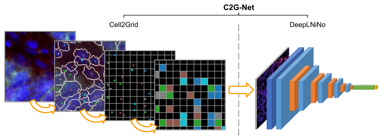
In this section we describe our method, C2G-Net (see Figure 1), which consists of two components: Cell2Grid, an image compression algorithm that exploits the morphological properties of a specific class of images and DeepLNiNo, a CNN architecture designed to operate on these compressed images. Our method is applicable to images that contain a large number of similar objects.

Figure 1: C2G-Net consisting of: (1) Cell2Grid, an image compression algorithm that significantly reduces training time and (2) DeepLNiNo, a CNN architecture designed to operate on Cell2Grid-compressed images and improve interpretability.

2.1 Cell2Grid image compression algorithm

The Cell2Grid image compression algorithm consists of the three steps listed below.

Step 1: Object identification
During the first step, relevant objects (e.g. biological cells) are identified in the image. For each object, its location within the image as well as other relevant properties for the image analysis task (e.g. average color, size, or shape of the object) are extracted. The final output of the object identification step is therefore a list of objects with their associated xy-coordinates $\vec{X}$ and properties, similar to point-cloud data.

Step 2: Assigning objects to target grid
The goals of Step 2 are to first obtain a target grid that is virtually placed over the images and then place objects from Step 1 on that target grid.

The target grid is a square grid with grid spacing $d$ in units of image pixels and it should be as coarse as possible (to achieve a high compression ratio) while simultaneously being as fine as necessary to prevent that grid locations become overpopulated by objects (i.e., an excessive amount of assignment conflicts).

As a simple heuristic for estimating a suitable target grid spacing $d$, we use

$$d\approx\frac{1}{2}\left(\frac{1}{n}\sum_{i=1}^{n}\sqrt{1/\rho_{i}}\right),$$ (1)

where $\rho_{i}$ is the object density of image $i$ and the sum includes all images to be compressed in a single batch. The square root in Equation 1 transforms the inverse of the object density (the average area occupied by each object) into a spatial dimension, estimating the average object extent. After averaging over all $n$ images in the batch, we divide by $2$ to account for possible empty space in the images and local density variations. If desired, the computed value can be rounded to the next integer to ease explainability and visualization of the compressed images.

Once grid spacing is calculated, all identified objects are assigned to the target grid by binning their original xy-coordinates $\vec{X}$ to the discrete nodes of the target grid:

$$\vec{X}_{g}=\lfloor\vec{X}/d\rceil,$$ (2)

whereas the $\lfloor\cdot\rceil$ denotes conventional rounding to the next integer and $\vec{X}_{g}$ corresponds to the coordinates of pixels in the final compressed image.

If two objects are within a distance of $d\sqrt{2}$ they may be assigned to the same $\vec{X}_{g}$. To achieve a one-to-one relation of objects to pixels, we require that each object is assigned uniquely to a grid node. Therefore, possible assignment conflicts are resolved by either moving objects to free adjacent grid nodes or by deleting them from the data. In Appendix A, we introduce PriorityShift, a simple algorithm that resolves conflicts locally in a computationally efficient way. After this step, nodes in the target grid are either empty or contain exactly one object and its associated properties.

Step 3: Image compression
In Step 3, a low-resolution compressed output image is produced. After Step 2, grid nodes contain the properties of assigned objects, similarly to how pixels contain RGB color values in conventional images. In our case, the resulting data structure is a tensor of size $K_{x}\times K_{y}\times P$, where $K_{x}$ and $K_{y}$ are the number of grid lines in x and y dimension, respectively, and $P$ is the number of object features stored at each node. Grid nodes without objects are assigned zero as a default value for every object property. Since a square grid was used, our tensor can be converted into an image with $P$ color channels, e.g. by using a lossless image format with multiple channels, like multi-channel TIFF. This multiplex image, which we term Cell2Grid image, is the final output of the image compression step.

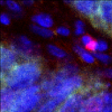
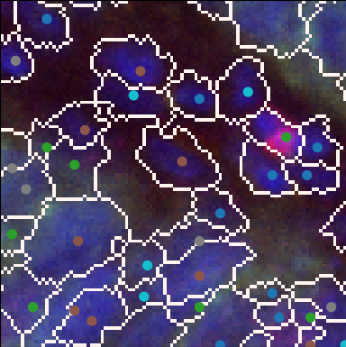
An example of the whole process for a biological image from our case study is introduced in subsection 3.1 (Figure 3).

2.2 DeepLNiNo CNN architecture

To exploit the special properties of Cell2Grid images (further information in the Discussion section) we experimented with different CNN architectures that are designed for spatially sparse input, with DeepCNet (Graham, 2014) and the Network-in-Network approach (Lin et al., 2013) being the most relevant for our task and the ones we built on. A DeepCNet(l,k) network consists of $l$ convolutional layers, each of which is followed by a max pooling layer. The number of feature maps in the convolutional layers increases from layer to layer, being $n\times k$ in layer $n$. While DeepCNet consists of one layer with filter size $3\times 3$ followed by several layers with filter size $2\times 2$, the Network-in-Network architecture also makes use of convolutional layers with filter size $1\times 1$.

Table 1: DeepLNiNo architecture.

type	filter size	output size	params
input		$135\times 101\times 6$
conv	$1\times 1$	$135\times 101\times 16$	112
conv	$2\times 2$	$134\times 100\times 16$	1,040
maxpool	$2\times 2$	$67\times 50\times 16$
conv	$3\times 3$	$65\times 48\times 16$	2,320
maxpool	$3\times 3$	$21\times 16\times 16$
conv	$3\times 3$	$19\times 14\times 16$	2,320
maxpool	$3\times 3$	$6\times 4\times 16$
conv	$3\times 3$	$6\times 4\times 16$	2,320
maxpool	$3\times 3$	$2\times 2\times 16$
conv	$2\times 2$	$2\times 2\times 16$	1,040
maxpool	$2\times 2$	$1\times 1\times 16$
flatten
dense		$1\times 1\times 32$	544
dropout	33%
softmax		$1\times 1\times 2$	66
params total			9,762

Our goal was to create a CNN architecture that has significantly fewer trainable parameters than comparable architectures and is easy to interpret while still performing well in a binary image classification task. For that purpose, we introduce Deep L1-regularized Network-in-Network narrOw (DeepLNiNo) architecture, an easy-to-interpret CNN designed to work with Cell2Grid images of size $135\text{\times}101\text{\,}\mathrm{px}$ and six color channels. DeepLNiNo is small (less than 10,000 trainable parameters), sparse (L1-regularization of the first convolutional layer with $1\times 1$-kernel) and narrow (only 16 filters per convolutional layer). Table 1 lists the network architecture.

In DeepLNiNo, each convolutional layer has 16 filters, with the first one using a kernel size of $1\times 1$, as inspired by the Network-in-Network approach. This layer is L1-regularized to introduce sparsity and increase model interpretability. Since one pixel in Cell2Grid images corresponds exactly to one object, this layer enables the tracking of learned object properties. The remaining convolutional layers use a mix of kernel sizes and image padding methods. Dropout (Hinton et al., 2012) is applied only after the fully connected dense layer. In total, DeepLNiNo consists of 9,762 trainable parameters.

2.3 Reference model

As a reference CNN architecture, we used a modification of the DeepCNet architecture proposed by Graham (2014) that was extended by a fully connected layer with 128 neurons at the end of the network. We used the parameters $l=6$ and $k=32$, resulting in a network with six convolutional layers, and $32\times n$ feature maps in convolutional layer $n$. We denote this model as DeepCNet(l=6) indicating the number of layers used while keeping $k=32$ for all models.

3 Case Study: Colon Cancer Relapse

To test the performance of C2G-Net, we used a real use case from health care: predicting the relapse risk of colon cancer patients. In a retrospective study, surgically removed tumor tissue samples from 48 colon cancer patients were collected from a biobank. Each patient was observed for at least 3 years after tumor surgery and their final tumor recurrence status labeled as either relapse (12 patients, 25%) or no-relapse (36 patients, 75%). The goal was to predict the final tumor recurrence status (i.e. relapse/no-relapse) for each single image.

We wanted to investigate (a) how two different CNN model architectures perform on Cell2Grid images, (b) how the three different types of input images (raw, RGB and Cell2Grid) at the same image resolution influence the performance of a single CNN model and (c) how training time differs for the best performing models on all three input image types.

3.1 Materials

Figure 2: The six different model configurations used in our experiment.

Images consisted of multiplex immunohistochemistry (mIHC) micrographs of formalin-fixed paraffin embedded (FFPE) tissue sections from the tumor (Fox et al., 1985) stained with six fluorescence-conjugated antibodies (CD3, CD8, CD45RO, PD-L1, FoxP3, Her2 plus DAPI for staining the nuclei of the cells) (Ramos-Vara & Miller, 2014). Images covered an area of $672\text{\times}504\text{\,}\mathrm{\SIUnitSymbolMicro m}$ and were recorded at 40x magnification, with a final size of $1,344\text{\times}1,008\text{\,}\mathrm{px}$ at a $0.5\text{\,}\mathrm{\SIUnitSymbolMicro}\mathrm{m}\mathrm{/}\mathrm{px}$ resolution and six color channels, one for each antibody used. 1,119 mIHC images from the 48 patients were recorded in total. These images are referred to as raw images.

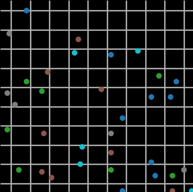
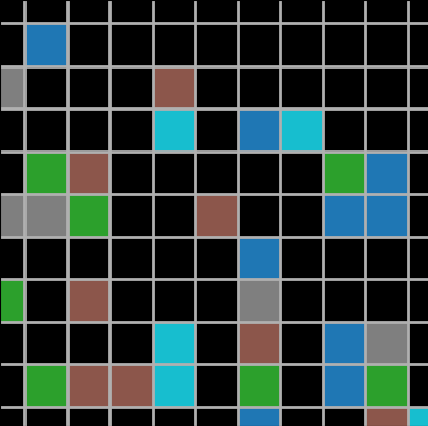
Based on this set of raw images, we created two additional data sets termed RGB and Cell2Grid. RGB images are pseudo-color images where the six color channels of the raw image are mapped to distinct RGB color values. Figure 3 illustrates the compression of raw images using Cell2Grid. For object identification we used inForm (Akoya Biosciences, 2019), a commercially available software for biological cell segmentation. On average, images contained 4,149 biological cells in an area of $338,688\text{\,}{\mathrm{\SIUnitSymbolMicro m}}^{2}$ ($\approx$$81.6\text{\,}\mathrm{\SIUnitSymbolMicro}\mathrm{m}\mathrm{{}^{2}}\mathrm{/}\mathrm{cell}$). For all six recorded IHC markers, the average color channel intensities (i.e. marker expressions) over the entire cell area were calculated and used as object properties. We calculated the target grid spacing according to Equation 1 using all images to be $d=$ $4.7\text{\,}\mathrm{\SIUnitSymbolMicro m}$ $\approx$ $5\text{\,}\mathrm{\SIUnitSymbolMicro m}$. This is comparable to the size of a lymphocyte (Wood, 2004). We used the location of the cells nuclei as point-like object locations for assignment to the grid. Assignment conflicts were resolved with PriorityShift.

Figure 3: Cell2Grid image compression procedure and final outcome. (a) Small part of a raw image, visualized as RGB image ($100\times 100$ pixels covering an area of $50\text{\times}50\text{\,}\mathrm{\SIUnitSymbolMicro m}$); (b) outlines of the identified objects (biological cells) in white and dots with random colors showing the locations of the cells nuclei; (c) point-like locations of objects with superimposed target grid with grid spacing $d=$ $5\text{\,}\mathrm{\SIUnitSymbolMicro m}$; (d) final Cell2Grid image ($10\times 10$ pixels); assignment conflicts (e.g. green and gray cell in the bottom right corner) resolved with PriorityShift. The final Cell2Grid image is sparse, containing several completely black pixels, even in regions with many objects.

3.2 Methods and Evaluation

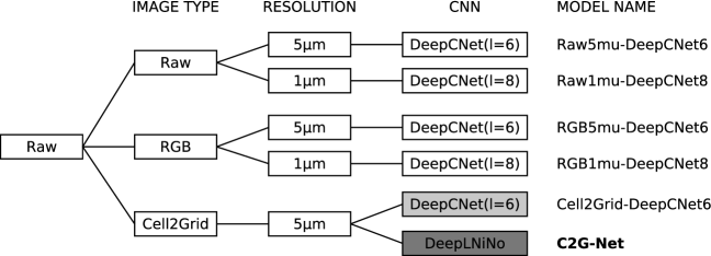
We created 6 different models by combining image type (raw, RGB, and Cell2Grid), resolution ($1\text{\,}\mathrm{\SIUnitSymbolMicro m}$ and $5\text{\,}\mathrm{\SIUnitSymbolMicro m}$), and CNN (DeepCNet and DeepLNiNo)—see Figure 2. Raw and RGB images were rescaled to $5\text{\,}\mathrm{\SIUnitSymbolMicro m}$ and $1\text{\,}\mathrm{\SIUnitSymbolMicro m}$ using bilinear interpolation (Clark, 2015) and the number of layers in DeepCNet adapted to accommodate for image size. We implemented all models in Python using Keras (Chollet et al., 2015) and trained on a conventional desktop workstation with one GPU (Nvidia RTX 2070).

Each model was trained 10 times to estimate model variance and all $n=1,119$ images split into a training and a validation set ($2/3$ and $1/3$ of images, respectively) by stratifying samples based on their relapse class. Training images were oversampled to account for class imbalance. To further emphasize the clinical importance of predicting the relapse class, we weighted corresponding samples by 3:1 in favour of relapse, and used standard data augmentation to avoid overfitting. For Cell2Grid images, we had to implement our own data augmentation methods due to the special properties of Cell2Grid images (see Appendix B for details). Cross entropy was used as loss function and Adadelta (Zeiler, 2012) as optimizer.

3.3 Results

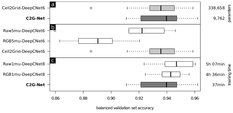
We experimented with the number of training epochs and found that all DeepCNet models fully converged after 400 epoch while the DeepLNiNo model required 1000 epochs, likely an effect of L1-regularization. Table 2 shows the mean and standard deviation for balanced validation set accuracy and training times for the 10 runs per model, results are illustrated in Figure 4. Figure 4a shows that both DeepLNiNo and DeepCNet perform equally well when trained on Cell2Grid images, although DeepLNiNo contains significantly fewer trainable parameters. Using the same DeepCNet architecture with different input data types, Figure 4b shows that using Cell2Grid images leads to the most accurate models.

Finally, Figure 4c compares the best models for each input data type. While C2G-Net can not outperform the models using data at $1\text{\,}\mathrm{\SIUnitSymbolMicro m}$ resolution, the required training time was reduced by more than a 85%. As expected, a general trend towards worse performance with decreasing input image resolution can be observed for both raw and RGB images.

Table 2: Mean (standard deviation) for balanced validation set accuracy for 10 model runs and average training time of a single run for different CNN architectures and input data types. Image resolution denotes the resolution of images for training after compression.

Model name	Image type	Image res.	CNN	Bal. accuracy	Training time
Raw5mu-DeepCNet6	Raw	$5\text{\,}\mathrm{\SIUnitSymbolMicro m}$	DeepCNet(l=6)	0.921 (0.024)	00:07:29
Raw1mu-DeepCNet8	Raw	$1\text{\,}\mathrm{\SIUnitSymbolMicro m}$	DeepCNet(l=8)	0.946 (0.014)	05:07:23
RGB5mu-DeepCNet6	RGB	$5\text{\,}\mathrm{\SIUnitSymbolMicro m}$	DeepCNet(l=6)	0.891 (0.019)	00:03:54
RGB1mu-DeepCNet8	RGB	$1\text{\,}\mathrm{\SIUnitSymbolMicro m}$	DeepCNet(l=8)	0.942 (0.011)	04:36:18
Cell2Ggrid-DeepCNet6	Cell2Grid	$5\text{\,}\mathrm{\SIUnitSymbolMicro m}$	DeepCNet(l=6)	0.932 (0.021)	00:07:48
C2G-Net (our method)	Cell2Grid	$5\text{\,}\mathrm{\SIUnitSymbolMicro m}$	DeepLNiNo	0.938 (0.017)	00:37:31

Figure 4: Balanced validation set accuracy of 10 model runs each, see Table 2. (a) Comparison of CNN architectures using Cell2Grid images; (b) Comparison of different input data types using DeepCNet architecture; (c) comparison of best models for each input data type. C2G-Net in dark gray, Cell2Grid-DeepCNet in light gray.

4 Discussion

In recent years, CNN architectures have become increasingly large, requiring long training times and powerful hardware, particularly when using large images for training (Krizhevsky et al., 2012; Szegedy et al., 2014; Simonyan & Zisserman, 2014; He et al., 2015). However, when images contain a large number of similar objects, their morphological properties can be exploited by using a compressed representation of their individual objects placed on a grid. These compressed images can then be used to train a CNN, as long as their special properties are taken into account.

4.1 Properties of Cell2Grid images

Cell2Grid images are different from conventional images in a number of ways: (1) they contain no natural gradients, since every pixel in the image is an independent object (e.g., a biological cell); (2) they might contain many empty pixels (numerically zero) in areas without assigned objects during compression; and (3) they can not be arbitrarily rotated, zoomed, sheared or transformed for data augmentation purposes, since the value and integrity of individual pixels matter (see Appendix B).

As previously shown in Figure 3, the final Cell2Grid image is sparse, containing several completely black pixels, even in regions with many objects. While cells surrounded by background tend to vanish in conventional downscaling due to averaging with background pixels, they are conserved during Cell2Grid compression. In this example, the Cell2Grid image has 10-times fewer pixels in each spatial direction, corresponding to a compression ratio of 100.

The Cell2Grid image compression algorithm is related to the concept of superpixels (Bechar et al., 2019; Akbar et al., 2015). However, while superpixels are typically used to segment the whole image into regions of similarity (including background and irrelevant objects), Cell2Grid focuses on relevant objects only and keeps their integrity intact. Compared to Voronoi tessellation (Chen et al., 2017) and graph-based methods (Chen et al., 2017) based on superpixels, our proposed places all identified objects on a target grid by approximating the location of each object to fit the grid. The final data format is that of a conventional, multi-channel image.

4.2 Model interpretation

Figure 5: Learned filter weights of the first convolutional layer with kernel size $1\times 1$ of a trained DeepLNiNo model. Higher values indicate increased importance of a channel for a given filter. For ease of interpretation, all negative filter weights have been colored in the same color.

Although some progress has been made towards explaining a trained CNN (Zeiler & Fergus, 2014; Mahendran & Vedaldi, 2015; Zhang et al., 2018; Ribeiro et al., 2016), keeping model architectures simple makes them easier to train and simplifies the extraction of knowledge (Kaya et al., 2018). In contrast to other popular CNN model architectures that have become very deep and wide, resulting in several millions of trainable parameters (Krizhevsky et al., 2012; Szegedy et al., 2014; Simonyan & Zisserman, 2014; He et al., 2015), due to the narrow architecture of DeepLNiNo, the whole network and its learned weights can be displayed, facilitating interpretation.

Table 3: Comparison of size of training images and number of trainable parameters for C2G-Net and popular networks for image classification.

Model name	Raw input image size	File size (MB)	Parameters
C2G-Net (our method)	$1,344\text{\times}1,008\text{\times}6\text{\,}$	8.13	10k
GoogLeNet (Szegedy et al., 2014)	$224\text{\times}224\text{\times}3\text{\,}$	0.15	6,400k
ResNet-152 (He et al., 2015)	$224\text{\times}224\text{\times}3\text{\,}$	0.15	60,200k
AlexNet (Krizhevsky et al., 2012)	$224\text{\times}224\text{\times}3\text{\,}$	0.15	62,300k
VGG16 (Simonyan & Zisserman, 2014)	$224\text{\times}224\text{\times}3\text{\,}$	0.15	138,000k

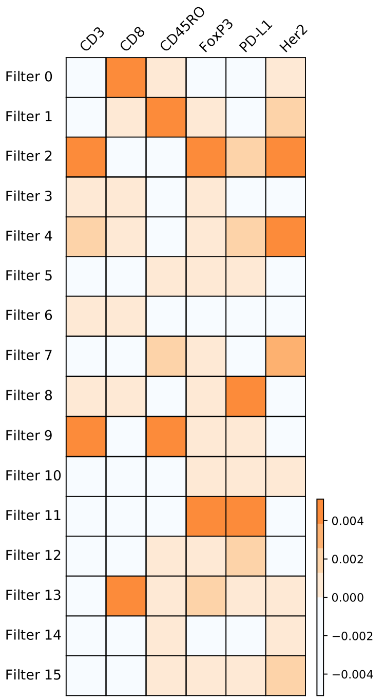
Since individual pixels correspond to objects in Cell2Grid images, learned filter weights in a neural network can be interpreted at an object level. Figure 5 shows the learned weights of the first convolutional layer of a trained DeepLNiNo model, consisting in 16 filters with kernel size 1x1. It can be seen that Filter 9 is strongly activated by cells containing high values of CD3, CD45RO, or both. This combination of markers is characteristic for memory T-cells, which have been found previously to play a role in colon cancer prognosis (Pagès et al., 2005). Furthermore, every IHC marker channel appears exactly twice in all filters with a weight above $0.004$, indicating that every color channel contains useful information for classification. As expected, L1-regularization introduced some level of sparsity to the weights. Out of all filters, only eight contain at least one weight above $0.004$.

This form of model interpretation on the level of individual objects is enabled by the Cell2Grid image compression. Other image downscaling methods, like the bi-linear interpolation used for our reference data types, destroy the integrity of the biological cells by merging pixels from several cells and background together, making model interpretation more difficult. However, we acknowledge that this form of single-layer interpretation of our current DeepLNiNo architecture has its limits, since all feature maps are combined in a non-linear fashion in the downstream layers.

Table 3 shows the number of parameters in DeepLNiNo (10,000) compared to other popular CNNs for image classification (6-138 million). While other model architectures (e.g. VGG (Simonyan & Zisserman, 2014)) employ pooling much slower, DeepLNiNo applies aggressive maxpooling after every convolutional layer (except for the first). Together with the image compression step of C2G-Net, the number of parameters is kept small while still allowing for much larger input images.

5 Future work

In our experiment, we used raw images of size $1,344\text{\times}1,008\text{\,}\mathrm{px}$. However, a whole-slide-image (WSI) of a tissue section can be up to 30 times bigger in each spatial dimension. Building on our findings, we plan on applying C2G-Net to WSI data to test its performance on very large images.

Compared to conventional images, the creation of artificial Cell2Grid images is simple due to their object-like properties. In order to improve the extraction of knowledge from trained CNNs, we aim at creating simulated Cell2Grid data for which the ground truth of image labels is known by design (e.g. a difference in relative cell phenotype counts, different spatial distribution patterns etc.). We hypothesize that simulated Cell2Grid data will foster knowledge extraction from trained CNNs, which is especially important for applications in biology and health care.

When working with conventional images, local interpretable model-agnostic explanations (LIME, (Ribeiro et al., 2016)) have been used to break down why a CNN makes certain predictions. To this end, LIME uses superpixels (Bechar et al., 2019; Akbar et al., 2015) and assess their contribution to the predictions. We plan on adapting LIME to work with Cell2Grid image data by occluding groups of similar objects instead of superpixels.

6 Other applications

In this paper we applied C2G-Net to biological data in form of mIHC images. However, we hypothesize that our approach can be used on other image data sets that contain a large number of similar objects, such those in biology, satellite imagery, astronomy and material sciences.

Finally, it is straightforward to extend the idea of C2G-Net to 3-dimensional data. For example, 2-dimensional images of consecutive sections of FFPE tissue (with slice thickness of $\approx$$4\text{\,}\mathrm{\SIUnitSymbolMicro m}$ (Robertson et al., 2008)) can be compressed with Cell2Grid by using a target grid spacing of the same width. By virtual stacking of these images, a 3-dimensional data model containing each object as a cube could be created. We hypothesize that training a 3-dimensional CNN on this data could further improve model performance.

7 Conclusion

In this paper, we investigated if the morphological properties of images containing a large number of similar objects like biological cells can be exploited for image classification. For this purpose, we introduced C2G-Net consisting of Cell2Grid, an image compression algorithm, and DeepLNiNo, a CNN architecture aimed at facilitating model interpretability.

As a case study, we investigated predicting relapse risk in colon cancer using multiplex immunohistochemistry images. We found that Cell2Grid alone improved prediction accuracy of a CNN compared to conventional image compression. Moreover, when comparing the entire C2G-Net pipeline to models trained on high resolution raw images, C2G-Net showed comparable prediction accuracy, reduced training time by more than 85%, and provided a model that is easier to interpret.

Appendix A PriorityShift: resolving assignment conflicts

During step 2 of Cell2Grid image compression, i.e. binning of objects to the target grid, several objects might be assigned to the same grid node $\vec{X}_{g}$. These conflicts become more frequent with increasing grid spacing $d$. A finer grid spacing might prevent such conflicts but also reduces the compression ratio of the algorithm. In any case, assignment conflicts need to be resolved to obtain a one-to-one mapping of objects to pixels. This can be achieved either by deleting conflicting objects or moving them to adjacent free grid nodes. Algorithm 1 introduces PriorityShift, a simple and fast method that resolves assignment conflicts while minimizing the amount of objects that need to be deleted.

To make this algorithm computationally efficient, we reduced the number of times that euclidean distances need to be calculated. For $n$ conflicting objects, we only calculate $n$ euclidean distances from each object to the conflicting grid node $G$. When determining which adjacent grid node is closest to an object, we exploit the geometry of the square grid by calculating in which of the eight quadrant halves around $G$ the object is located. This location directly determines the priority of adjacent grid nodes. The conflicting object is then shifted to the free grid node with highest priority.

Algorithm 1 PriorityShift

  Input: grid with assigned objects containing assignment conflicts

  for every grid node $G$ with conflicting objects do

     get original locations of objects conflicting at $G$

     sort conflicting objects by proximity to $G$

     get list $L$ of free grid nodes directly adjacent to $G$

     assign the object closest to $G$ to grid node $G$

     for remaining conflicting objects at $G$ do

        if L contains at least one element then

           determine priority of grid nodes in $L$

           assign objects to node in $L$ with highest priority

           update $L$

        else

           delete object from the data

        end if

     end for

  end for

  Output: grid with assigned objects without conflicts

Appendix B Data augmentation for Cell2Grid images

To prevent CNNs from overfitting (Wong et al., 2016; Taylor & Nitschke, 2017), a multitude of data augmentation methods for conventional images are available, including translations, rotations, zooming, shearing and others (Chollet et al., 2015; Bloice et al., 2019). However, Cell2Grid images are different from conventional images, as outlined in the main text. Therefore, traditional image augmentation methods are not applicable or need to be modified. On the other hand, new augmentation methods specific to Cell2Grid images can be used.

We used the following data augmentation methods for Cell2Grid images of size $135\text{\times}101\text{\,}\mathrm{px}$. Each method was applied with probability $p$ to an image during training:

• Translations ($p=100\%$). We translated images horizontally (max. $30\text{\,}\mathrm{px}$) and vertically (max. $20\text{\,}\mathrm{px}$).

• Reflections ($p=100\%$). We performed horizontal and/or vertical reflections.

• Discrete rotations ($p=100\%$). We rotated images around $0\text{\,}\mathrm{\SIUnitSymbolDegree}$, $90\text{\,}\mathrm{\SIUnitSymbolDegree}$, $180\text{\,}\mathrm{\SIUnitSymbolDegree}$ or $270\text{\,}\mathrm{\SIUnitSymbolDegree}$.

• Blackouts ($p=80\%$). We deleted all objects in an area of $25\text{\times}25\text{\,}\mathrm{px}$ at a random location.

• Local pixel shuffle ($p=100\%$). For 50 random locations, we shuffled the objects in an area of $3\text{\times}3\text{\,}\mathrm{px}$.

• Channel brightness change ($p=10\%$). We changed the brightness of each color channel individually by multiplication of all values with a random factor in the range $[0.9,1.1]$.

• Global brightness change ($p=100\%$). We changed the brightness of all channels together with a random factor in the range $[0.8,1.2]$.

• Deleting pixels ($p=100\%$). We randomly chose 100 pixels and set their values to 0.

Where applicable, we used the ”reflect” mode of Keras to fill empty pixels, otherwise we filled occurring empty pixels with $0$.

References

- Akbar et al. (2015) Akbar, S., Jordan, L., Thompson, A. M., and McKenna, S. J. Tumor localization in tissue microarrays using rotation invariant superpixel pyramids. In 2015 IEEE 12th International Symposium on Biomedical Imaging (ISBI), pp. 1292–1295. ieeexplore.ieee.org, April 2015.
- Akoya Biosciences (2019) Akoya Biosciences. inform tissue finder :: Akoya. https://www.akoyabio.com/phenopticstm/software/inform-tissue-finder, 2019. Accessed: 2019-11-19.
- Bechar et al. (2019) Bechar, M. E. A., Settouti, N., Daho, M. E. H., Adel, M., and Chikh, M. A. Influence of normalization and color features on super-pixel classification: application to cytological image segmentation. Australas. Phys. Eng. Sci. Med., 42(2):427–441, June 2019.
- Bloice et al. (2019) Bloice, M. D., Roth, P. M., and Holzinger, A. Biomedical image augmentation using augmentor. Bioinformatics, 35(21):4522–4524, November 2019.
- Bulten et al. (2019) Bulten, W., Bándi, P., Hoven, J., Loo, R. v. d., Lotz, J., Weiss, N., Laak, J. v. d., van Ginneken, B., Hulsbergen-van de Kaa, C., and Litjens, G. Epithelium segmentation using deep learning in H&E-stained prostate specimens with immunohistochemistry as reference standard. Sci. Rep., 9(1):864, January 2019.
- Chen et al. (2017) Chen, J.-M., Li, Y., Xu, J., Gong, L., Wang, L.-W., Liu, W.-L., and Liu, J. Computer-aided prognosis on breast cancer with hematoxylin and eosin histopathology images: A review. Tumour Biol., 39(3):1010428317694550, March 2017.
- Chollet et al. (2015) Chollet, F. et al. Keras. https://github.com/fchollet/keras, 2015.
- Clark (2015) Clark, A. Pillow (PIL fork) documentation, 2015.
- Fox et al. (1985) Fox, C. H., Johnson, F. B., Whiting, J., and Roller, P. P. Formaldehyde fixation. J. Histochem. Cytochem., 33(8):845–853, August 1985.
- Gertych et al. (2019) Gertych, A., Swiderska-Chadaj, Z., Ma, Z., Ing, N., Markiewicz, T., Cierniak, S., Salemi, H., Guzman, S., Walts, A. E., and Knudsen, B. S. Convolutional neural networks can accurately distinguish four histologic growth patterns of lung adenocarcinoma in digital slides. Sci. Rep., 9(1):1483, February 2019.
- Goodfellow et al. (2016) Goodfellow, I., Bengio, Y., and Courville, A. Deep Learning. MIT Press, November 2016.
- Graham (2014) Graham, B. Spatially-sparse convolutional neural networks. arXiv e-prints, art. arXiv:1409.6070, Sep 2014.
- He et al. (2015) He, K., Zhang, X., Ren, S., and Sun, J. Deep residual learning for image recognition. arXiv e-prints, December 2015.
- Hinton et al. (2012) Hinton, G. E., Srivastava, N., Krizhevsky, A., Sutskever, I., and Salakhutdinov, R. R. Improving neural networks by preventing co-adaptation of feature detectors. arXiv e-prints, July 2012.
- Hofman et al. (2019) Hofman, P., Badoual, C., Henderson, F., Berland, L., Hamila, M., Long-Mira, E., Lassalle, S., Roussel, H., Hofman, V., Tartour, E., and Ilié, M. Multiplexed immunohistochemistry for molecular and immune profiling in lung Cancer-Just about ready for Prime-Time? Cancers, 11(3), February 2019.
- Kather et al. (2019) Kather, J. N., Krisam, J., Charoentong, P., Luedde, T., Herpel, E., Weis, C.-A., Gaiser, T., Marx, A., Valous, N. A., Ferber, D., Jansen, L., Reyes-Aldasoro, C. C., Zörnig, I., Jäger, D., Brenner, H., Chang-Claude, J., Hoffmeister, M., and Halama, N. Predicting survival from colorectal cancer histology slides using deep learning: A retrospective multicenter study. PLoS Med., 16(1):e1002730, 2019.
- Kaya et al. (2018) Kaya, Y., Hong, S., and Dumitras, T. Shallow-Deep networks: Understanding and mitigating network overthinking. arXiv e-prints, October 2018.
- Khosravi et al. (2018) Khosravi, P., Kazemi, E., Imielinski, M., Elemento, O., and Hajirasouliha, I. Deep convolutional neural networks enable discrimination of heterogeneous digital pathology images. EBioMedicine, 27:317–328, January 2018.
- Komura & Ishikawa (2018) Komura, D. and Ishikawa, S. Machine learning methods for histopathological image analysis. Comput. Struct. Biotechnol. J., 16:34–42, February 2018.
- Krizhevsky et al. (2012) Krizhevsky, A., Sutskever, I., and Hinton, G. E. ImageNet classification with deep convolutional neural networks. In Pereira, F., Burges, C. J. C., Bottou, L., and Weinberger, K. Q. (eds.), Advances in Neural Information Processing Systems 25, pp. 1097–1105. Curran Associates, Inc., 2012.
- Lin et al. (2013) Lin, M., Chen, Q., and Yan, S. Network in network. arXiv e-prints, December 2013.
- Liu et al. (2017) Liu, Y., Gadepalli, K., Norouzi, M., Dahl, G. E., Kohlberger, T., Boyko, A., Venugopalan, S., Timofeev, A., Nelson, P. Q., Corrado, G. S., Hipp, J. D., Peng, L., and Stumpe, M. C. Detecting cancer metastases on gigapixel pathology images. arXiv e-prints, March 2017.
- Mahendran & Vedaldi (2015) Mahendran, A. and Vedaldi, A. Understanding deep image representations by inverting them. In Proceedings of the IEEE conference on computer vision and pattern recognition, pp. 5188–5196, 2015.
- Mungle et al. (2017) Mungle, T., Tewary, S., Das, D. K., Arun, I., Basak, B., Agarwal, S., Ahmed, R., Chatterjee, S., and Chakraborty, C. MRF-ANN: a machine learning approach for automated ER scoring of breast cancer immunohistochemical images. J. Microsc., 267(2):117–129, 2017.
- Ozge Unel et al. (2019) Ozge Unel, F., Ozkalayci, B. O., and Cigla, C. The power of tiling for small object detection. In Proceedings of the IEEE Conference on Computer Vision and Pattern Recognition Workshops, pp. 0–0, 2019.
- Pagès et al. (2005) Pagès, F., Berger, A., Camus, M., Sanchez-Cabo, F., Costes, A., Molidor, R., Mlecnik, B., Kirilovsky, A., Nilsson, M., Damotte, D., Meatchi, T., Bruneval, P., Cugnenc, P.-H., Trajanoski, Z., Fridman, W.-H., and Galon, J. Effector memory T cells, early metastasis, and survival in colorectal cancer. N. Engl. J. Med., 353(25):2654–2666, December 2005.
- Parra et al. (2019) Parra, E. R., Francisco-Cruz, A., and Wistuba, I. I. State-of-the-art of profiling immune contexture in the era of multiplexed staining and digital analysis to study paraffin tumor tissues. Cancers, 11(2), 2019.
- Pinckaers & Litjens (2018) Pinckaers, H. and Litjens, G. Training convolutional neural networks with megapixel images. arXiv e-prints, April 2018.
- Ramos-Vara & Miller (2014) Ramos-Vara, J. A. and Miller, M. A. When tissue antigens and antibodies get along: revisiting the technical aspects of immunohistochemistry–the red, brown, and blue technique. Vet. Pathol., 51(1):42–87, January 2014.
- Ratner (2018) Ratner, M. FDA backs clinician-free AI imaging diagnostic tools. Nat. Biotechnol., 36(8):673–674, August 2018.
- Ribeiro et al. (2016) Ribeiro, M. T., Singh, S., and Guestrin, C. “why should I trust you?”: Explaining the predictions of any classifier. arXiv e-prints, February 2016.
- Robertson et al. (2008) Robertson, D., Savage, K., Reis-Filho, J. S., and Isacke, C. M. Multiple immunofluorescence labelling of formalin-fixed paraffin-embedded (FFPE) tissue. BMC Cell Biology, 9(1):13, 2008.
- Russakovsky et al. (2015) Russakovsky, O., Deng, J., Su, H., Krause, J., Satheesh, S., Ma, S., Huang, Z., Karpathy, A., Khosla, A., Bernstein, M., Berg, A. C., and Fei-Fei, L. ImageNet large scale visual recognition challenge. Int. J. Comput. Vis., 115(3):211–252, December 2015.
- Simonyan & Zisserman (2014) Simonyan, K. and Zisserman, A. Very deep convolutional networks for Large-Scale image recognition. arXiv e-prints, September 2014.
- Stack et al. (2014) Stack, E. C., Wang, C., Roman, K. A., and Hoyt, C. C. Multiplexed immunohistochemistry, imaging, and quantitation: a review, with an assessment of tyramide signal amplification, multispectral imaging and multiplex analysis. Methods, 70(1):46–58, November 2014.
- Szegedy et al. (2014) Szegedy, C., Liu, W., Jia, Y., Sermanet, P., Reed, S., Anguelov, D., Erhan, D., Vanhoucke, V., and Rabinovich, A. Going deeper with convolutions. arXiv e-prints, September 2014.
- Taylor & Nitschke (2017) Taylor, L. and Nitschke, G. Improving deep learning using generic data augmentation. arXiv e-prints, August 2017.
- Wang et al. (2015) Wang, D., Foran, D. J., Ren, J., Zhong, H., Kim, I. Y., and Qi, X. Exploring automatic prostate histopathology image gleason grading via local structure modeling. Conf. Proc. IEEE Eng. Med. Biol. Soc., 2015:2649–2652, 2015.
- Wong et al. (2016) Wong, S. C., Gatt, A., Stamatescu, V., and McDonnell, M. D. Understanding data augmentation for classification: When to warp? In 2016 International Conference on Digital Image Computing: Techniques and Applications (DICTA), pp. 1–6. ieeexplore.ieee.org, November 2016.
- Wood (2004) Wood, E. J. Cellular and molecular immunology (5th ed.): Abbas a. k., and lichtman, a. H. Biochem. Mol. Biol. Educ., 32(1):65–66, January 2004.
- Xu et al. (2016) Xu, J., Luo, X., Wang, G., Gilmore, H., and Madabhushi, A. A deep convolutional neural network for segmenting and classifying epithelial and stromal regions in histopathological images. Neurocomputing, 191:214–223, May 2016.
- Zeiler (2012) Zeiler, M. D. ADADELTA: An adaptive learning rate method. arXiv e-prints, December 2012.
- Zeiler & Fergus (2014) Zeiler, M. D. and Fergus, R. Visualizing and understanding convolutional networks. In Computer Vision – ECCV 2014, pp. 818–833. Springer International Publishing, 2014.
- Zhang et al. (2018) Zhang, Q., Nian Wu, Y., and Zhu, S.-C. Interpretable convolutional neural networks. In Proceedings of the IEEE Conference on Computer Vision and Pattern Recognition, pp. 8827–8836, 2018.