A 2×\times2 random switching model and its dual risk model

Anita Behme  and Philipp Strietzel Technische Universität Dresden, Institut für Mathematische Stochastik, Zellescher Weg 12-14, 01069 Dresden, Germany, anita.behme@tu-dresden.de and philipp.strietzel@tu-dresden.de, phone: +49-351-463-32425, fax: +49-351-463-37251.
(March 4, 2024)
Abstract

In this article a special case of two coupled M/G/1-queues is considered, where two servers are exposed to two types of jobs that are distributed among the servers via a random switch. In this model the asymptotic behavior of the workload buffer exceedance probabilities for the two single servers/ both servers together/ one (unspecified) server is determined. Hereby one has to distinguish between jobs that are either heavy-tailed or light-tailed. The results are derived via the dual risk model of the studied coupled M/G/1-queues for which the asymptotic behavior of different ruin probabilities is determined.

2020 Mathematics subject classification. 60K25, 94C11 (primary), 60G10, 91G05 (secondary)

Keywords: bipartite network, bivariate compound Poisson process, hitting probability, coupled M/G/1-queues, random switch, regular variation, ruin theory, queueing theory

1 Introduction

A general 2×2222\times 2 switch is modelled by a two-server queueing system with two arrival streams. A well-studied special cases of such a switch is given by the 2×2222\times 2 clocked buffered switch, where in a unit time interval each arrival stream can generate only one arrival and each server can serve only one customer; see e.g. [1, 11, 19] and others. This switch is commonly used to model a device used in data-processing networks for routing messages from one node to another.

In this paper we study a 2×2222\times 2 switch that operates in continuous time, i.e. the arrivals are modelled by two independent compound Poisson processes. Every incoming job is of random size and it is then distributed to the two servers by a random procedure. This leads to a pair of coupled M/G/1-queues. In this model we study the equilibrium probabilities of the resulting workload processes. In particular we determine the asymptotic behavior of the probabilities that the workloads exceed a prespecified buffer. Hereby we will distinguish between workload exceedance of a specific single server, both servers, or one unspecified server. As we will see, the behavior of these workload exceedance probabilities strongly depends on whether jobs are heavy-tailed or light-tailed and we will therefore consider both cases separately.

A related model to the one we study has been introduced in [10] where a pair of coupled queues driven by independent spectrally-positive Lévy processes is introduced. The coupling procedure however is completely different to the switch we shall use. For this model, in [10], the joint transform of the stationary workload distribution in terms of Wiener-Hopf factors is determined. Two parallel queues are also considered e.g. in [23] for an M/M/2-queue where arriving customers simultaneously place two demands handled independently by two servers. We refer to [2] and [22] and references therein for more general information on Lévy-driven queueing systems.

As it is well known, there are several connections between queueing and risk models. In particular the workload (or waiting time) in an M/G/1 queue with compound Poisson input is related to the ruin probability in the prominent Cramér-Lundberg risk model, in which the arrival process of claims is defined to be just the same compound Poisson process; see e.g. [2] or [31]. To be more precise, let

R(t)=u+cti=1N(t)Xi,t0,formulae-sequence𝑅𝑡𝑢𝑐𝑡superscriptsubscript𝑖1𝑁𝑡subscript𝑋𝑖𝑡0R(t)=u+ct-\sum_{i=1}^{N(t)}X_{i},\quad t\geq 0,

be a Cramér-Lundberg risk process with initial capital u>0𝑢0u>0, premium rate c>0𝑐0c>0, i.i.d. claims {Xi,i}subscript𝑋𝑖𝑖\{X_{i},i\in\mathbb{N}\} with cdf F𝐹F such that X1>0subscript𝑋10X_{1}>0 a.s. and 𝔼[X1]=μ<𝔼delimited-[]subscript𝑋1𝜇\mathbb{E}[X_{1}]=\mu<\infty, and a claim number process (N(t))t0subscript𝑁𝑡𝑡0(N(t))_{t\geq 0} which is a Poisson process with rate λ>0𝜆0\lambda>0. Then it is well known that the ruin probability

Ψ(u)=(R(t)<0for some t0)Ψ𝑢formulae-sequence𝑅𝑡0for some 𝑡0\Psi(u)=\mathbb{P}(R(t)<0\quad\text{for some }t\geq 0)

tends to 00 as u𝑢u\to\infty, as long as the net-profit condition λμ<c𝜆𝜇𝑐\lambda\mu<c holds, while otherwise Ψ(u)1Ψ𝑢1\Psi(u)\equiv 1. In particular, if the claims sizes are light-tailed in the sense that an adjustment coefficient κ>0𝜅0\kappa>0 exists, i.e.

κ>0:0eκxF¯(x)dx=cλ,\exists\kappa>0:\quad\int_{0}^{\infty}e^{\kappa x}\overline{F}(x)\mathop{}\!\mathrm{d}x=\frac{c}{\lambda},

where F¯(x)=1F(x)¯𝐹𝑥1𝐹𝑥\overline{F}(x)=1-F(x) is the tail-function of the claim sizes, then the ruin probability Ψ(u)Ψ𝑢\Psi(u) satisfies the famous Cramér-Lundberg inequality (cf. [2, Eq. XIII (5.2)], [3, Eq. I.(4.7)])

Ψ(u)eκu,u>0.formulae-sequenceΨ𝑢superscript𝑒𝜅𝑢𝑢0\Psi(u)\leq e^{-\kappa u},\quad u>0.

Furthermore in this case the Cramér-Lundberg approximation states that (cf. [2, Thm. XIII.5.2], [3, Eq. I.(4.3)])

limueκuΨ(u)=C,subscript𝑢superscript𝑒𝜅𝑢Ψ𝑢𝐶\lim_{u\to\infty}e^{\kappa u}\Psi(u)=C,

for some known constant C0𝐶0C\geq 0 depending on the chosen parameters of the model. On the contrary, for heavy-tailed claims with a subexponential integrated tail function 1μ0xF¯(y)dy1𝜇superscriptsubscript0𝑥¯𝐹𝑦differential-d𝑦\frac{1}{\mu}\int_{0}^{x}\overline{F}(y)\mathop{}\!\mathrm{d}y it is known that (cf. [3, Thm. X.2.1])

limu(1μuF¯(y)dy)1Ψ(u)=λμcλμ,subscript𝑢superscript1𝜇superscriptsubscript𝑢¯𝐹𝑦differential-d𝑦1Ψ𝑢𝜆𝜇𝑐𝜆𝜇\lim_{u\to\infty}\left(\frac{1}{\mu}\int_{u}^{\infty}\overline{F}(y)\mathop{}\!\mathrm{d}y\right)^{-1}\Psi(u)=\frac{\lambda\mu}{c-\lambda\mu},

and in the special case of tail-functions that are regularly varying this directly implies that the ruin probability decreases polynomially.
Via the mentioned duality these results can easily be translated into corresponding results on the workload exceedance probability of an M/G/1-queue.

In this paper we shall use an analogue duality between queueing and risk models in a multi-dimensional setting as it was introduced in [7]. This allows us to obtain results on the workload exceedance probabilities of the 2×2222\times 2 switch by studying the corresponding ruin probabilities in the two-dimensional dual risk model.

Bivariate risk models are a well-studied field of research. A prominent model in the literature, that can be interpreted as a special case of the dual risk model in this paper, has been introduced by Avram et. al. [5]. In this so-called degenerate model a single claim process is shared via prespecified proportions between two insurers (see e.g. [4, 5, 6, 24, 26]). The model allows for a rescaling of the bivariate process that reduces the complexity to a one-dimensional ruin problem. Exact results and sharp asymptotics for this model have been obtained in [4], where also the asymptotic behavior of ruin probabilities of a general two-dimensional Lévy model under light-tail assumptions is derived. In [24] the degenerate model is studied in the presence of heavy tails; specifically asymptotic formulae for the finite time as well as the infinite time ruin probabilities under the assumption of subexponential claims are provided. In [26] the degenerate model is extended by a constant interest rate. In [6] another generalization of the degenerate model is studied that introduces a second source of claims only affecting one insurer. Our risk model defined in Section 2.2 can be seen as a further generalization of the model in [6] because of the random sharing of every single claim, compare also with Section 5.2 below.
There exist plenty of other papers concerning bivariate risk models of all types and several approaches to tackle the problem. E.g. [14, 21] consider bivariate risk models of Cramér-Lundberg-type with correlated claim-counting processes and derive partial integro-differential equations for infinite-time ruin and survival probabilities in these models. Various authors focus on finite time ruin probabilities under different assumptions, see e.g. [15, 16, 17, 29, 32, 37, 38]. E.g. in [38] the finite time survival probability is approximated using a so-called bivariate compound binomial model and bounds for the infinite-time ruin probability are obtained using the concept of association.
In general dimensions, multivariate ruin is studied e.g. in [9, 12, 13, 25, 30, 34]. In particular, in [9] a bipartite network induces the dependence between the risk processes and this model is in some sense similar to the dual risk model in this paper. Further, in [20], multivariate risk processes with heavy-tailed claims are treated and so-called ruin regions are studied, that is, sets in dsuperscript𝑑\mathbb{R}^{d} which are hit by the risk process with small probability. Multivariate regularly varying claims are also assumed e.g. in [27] and [30], where in [27] several lines of business are considered that can balance out ruin, while [30] focuses exclusively on simultaneous ruin of all business lines/agents. Further, [36] introduces a notion of multivariate subexponentiality and applies this on a multivariate risk process. Note that [27] and [36] both consider rather general regions of ruin and some of the results from these papers will be applied on our dual risk model.

The paper is outlined as follows. In Section 2 we specify the random switch model that we are interested in and introduce the corresponding dual risk model. Section 3 is devoted to study both models under the assumption that jobs/claims are heavy-tailed and it is divided into two parts. First, in Section 3.1 we focus on subexponentiality. As we shall rely on results from [36] we first concentrate on the risk model in Section 3.1.1 and then transfer our findings to the switch model in Section 3.1.2. Second, we treat the special case of regular variation in Section 3.2, where we start with results for the risk model in Section 3.2.1, taking advantage of results given in [27], before we transfer our findings to the switch model in Section 3.2.2. In Section 4 we assume all jobs/claims to be light-tailed and again first consider the risk model in Section 4.1 before converting the results to the switch context in Section 4.2. Two particular examples of the switch will then be outlined in Section 5 where we also compare the behavior of the exceedance probabilities for different specifications of the random switch via a short simulation study in Section 5.3. The final Section 6 collects the proofs of all our findings.

2 The switching model and its dual

2.1 The 2×2222\times 2 random switching model

Let 𝒲1,𝒲2subscript𝒲1subscript𝒲2\mathcal{W}_{1},\mathcal{W}_{2} be servers (or workers) with work speeds c1,c2>0subscript𝑐1subscript𝑐20c_{1},c_{2}>0 and let 𝒥1,𝒥2subscript𝒥1subscript𝒥2\mathcal{J}_{1},\mathcal{J}_{2} be two job generating objects. We assume that both objects generate jobs independently with Poisson rates λ1,λ2>0subscript𝜆1subscript𝜆20\lambda_{1},\lambda_{2}>0, respectively, and that the workloads generated by one object are i.i.d. positive random variables. More specifically, we identify the objects 𝒥jsubscript𝒥𝑗\mathcal{J}_{j}, j=1,2𝑗12j=1,2, with two independent compound Poisson processes

k=1Nj(t)Xj,k,j=1,2formulae-sequencesuperscriptsubscript𝑘1subscript𝑁𝑗𝑡subscript𝑋𝑗𝑘𝑗12\sum_{k=1}^{N_{j}(t)}X_{j,k},\qquad j=1,2

with jumps {Xj,k,k}subscript𝑋𝑗𝑘𝑘\{X_{j,k},k\in\mathbb{N}\} being i.i.d. copies of two random variables XjFjsimilar-tosubscript𝑋𝑗subscript𝐹𝑗X_{j}\sim F_{j} such that Fj(0)=0subscript𝐹𝑗00F_{j}(0)=0 and 𝔼[Xj]<𝔼delimited-[]subscript𝑋𝑗\mathbb{E}[X_{j}]<\infty, j=1,2𝑗12j=1,2.

The jobs shall be distributed to the two servers by a random switch that is modeled by a random (2×2)22(2\times 2)-matrix 𝐀=(Aij)i,j=1,2𝐀subscriptsubscript𝐴𝑖𝑗formulae-sequence𝑖𝑗12\mathbf{A}=(A_{ij})_{i,j=1,2}, independent of all other randomness and satisfying the following conditions:

  1. (i)

    Aij[0,1]subscript𝐴𝑖𝑗01A_{ij}\in[0,1] for all i,j=1,2formulae-sequence𝑖𝑗12i,j=1,2, meaning that a job can not be assigned more than totally or less than not at all to a certain server,

  2. (ii)

    i=12Aij=1superscriptsubscript𝑖12subscript𝐴𝑖𝑗1\sum_{i=1}^{2}A_{ij}=1 for all j=1,2𝑗12j=1,2, i.e. every job must be assigned entirely to the servers.

The switch matrix is triggered independently at every arrival of a job.

𝒲1subscript𝒲1\mathcal{W}_{1}𝒲2subscript𝒲2\mathcal{W}_{2}𝒥1subscript𝒥1\mathcal{J}_{1}𝒥2subscript𝒥2\mathcal{J}_{2}c1subscript𝑐1c_{1}c2subscript𝑐2c_{2}𝐀ksubscript𝐀𝑘\mathbf{A}_{k}k=1N1(t)X1,ksuperscriptsubscript𝑘1subscript𝑁1𝑡subscript𝑋1𝑘\sum_{k=1}^{N_{1}(t)}X_{1,k}k=1N2(t)X2,ksuperscriptsubscript𝑘1subscript𝑁2𝑡subscript𝑋2𝑘\sum_{k=1}^{N_{2}(t)}X_{2,k}
Figure 1: The random switching model

We are interested in the coupled M/G/1𝑀𝐺1M/G/1-queues defined by the resulting storage processes of the two servers, i.e.

Wi(t)=j=12k=1Nj(t)(Aij)kXj,k0tci(Wi(s))dssubscript𝑊𝑖𝑡superscriptsubscript𝑗12superscriptsubscript𝑘1subscript𝑁𝑗𝑡subscriptsubscript𝐴𝑖𝑗𝑘subscript𝑋𝑗𝑘superscriptsubscript0𝑡subscript𝑐𝑖subscript𝑊𝑖𝑠differential-d𝑠W_{i}(t)=\sum_{j=1}^{2}\sum_{k=1}^{N_{j}(t)}(A_{ij})_{k}X_{j,k}-\int_{0}^{t}c_{i}(W_{i}(s))\mathop{}\!\mathrm{d}s (2.1)

where {𝐀k,k}subscript𝐀𝑘𝑘\{\mathbf{A}_{k},k\in\mathbb{N}\} are i.i.d. copies of 𝐀𝐀\mathbf{A} and

ci(x)={0,x0,ci,x>0,i=1,2.formulae-sequencesubscript𝑐𝑖𝑥cases0𝑥0subscript𝑐𝑖𝑥0𝑖12c_{i}(x)=\begin{cases}0,&x\leq 0,\\ c_{i},&x>0,\end{cases}\quad i=1,2.

In particular we aim to study the stationary distribution of the multivariate storage process 𝐖(t)=(W1(t),W2(t))𝐖𝑡superscriptsubscript𝑊1𝑡subscript𝑊2𝑡top\mathbf{W}(t)=(W_{1}(t),W_{2}(t))^{\top}, that is the distributional limit of 𝐖(t)𝐖𝑡\mathbf{W}(t) as t𝑡t\to\infty whenever it exists. In this case we write

𝐖:=(W1,W2)assign𝐖superscriptsubscript𝑊1subscript𝑊2top\mathbf{W}:=(W_{1},W_{2})^{\top} (2.2)

for a generic random vector with this steady-state distribution. Note that here and in the following ()superscripttop(\cdot)^{\top} denotes the transpose of a vector or matrix.

Let u>0𝑢0u>0 be some fixed buffer barrier for the system and 𝐛=(b1,b2)(0,1)2𝐛superscriptsubscript𝑏1subscript𝑏2topsuperscript012\mathbf{b}=(b_{1},b_{2})^{\top}\in(0,1)^{2} with b1+b2=1subscript𝑏1subscript𝑏21b_{1}+b_{2}=1. Set 𝐮=𝐛u𝐮𝐛𝑢\mathbf{u}=\mathbf{b}u, i.e. ui=biusubscript𝑢𝑖subscript𝑏𝑖𝑢u_{i}=b_{i}u. Then we are interested in the probabilities that the single servers exceed their barriers

Υi(ui)=(Wiui>0),i=1,2,formulae-sequencesubscriptΥ𝑖subscript𝑢𝑖subscript𝑊𝑖subscript𝑢𝑖0𝑖12\Upsilon_{i}(u_{i})=\mathbb{P}\left(W_{i}-u_{i}>0\right),\quad i=1,2, (2.3)

the probability that at least one of the workloads exceeds the barrier u𝑢u

Υ(u)=(maxi=1,2(Wiui)>0),subscriptΥ𝑢subscript𝑖12subscript𝑊𝑖subscript𝑢𝑖0\Upsilon_{\vee}(u)=\mathbb{P}\left(\max_{i=1,2}(W_{i}-u_{i})>0\right), (2.4)

and the probability that both of the workloads exceed the barrier u𝑢u

Υ(u)=(mini=1,2(Wiui)>0).subscriptΥ𝑢subscript𝑖12subscript𝑊𝑖subscript𝑢𝑖0\Upsilon_{\wedge}(u)=\mathbb{P}\left(\min_{i=1,2}(W_{i}-u_{i})>0\right). (2.5)

2.2 The dual risk model

In the one-dimensional case it is well known that there exists a duality between risk- and queueing models, see e.g. [2]. The multivariate analogue shown in [7] allows us to formulate the dual risk model to the above introduced random switching model as follows.

Let N(t):=N1(t)+N2(t)assign𝑁𝑡subscript𝑁1𝑡subscript𝑁2𝑡N(t):=N_{1}(t)+N_{2}(t) such that N(t)𝑁𝑡N(t) is a Poisson process with rate λ=λ1+λ2𝜆subscript𝜆1subscript𝜆2\lambda=\lambda_{1}+\lambda_{2}. Define the multivariate risk process

𝐑(t):=(R1(t)R2(t)):=k=1N(t)𝐀k𝐁k(X1,kX2,k)t(c1c2)=:k=1N(t)𝐀k𝐁k𝐗kt𝐜,\mathbf{R}(t):=\begin{pmatrix}R_{1}(t)\\ R_{2}(t)\end{pmatrix}:=\sum_{k=1}^{N(t)}\mathbf{A}_{k}\mathbf{B}_{k}\begin{pmatrix}X_{1,k}\\ X_{2,k}\end{pmatrix}-t\begin{pmatrix}c_{1}\\ c_{2}\end{pmatrix}=:\sum_{k=1}^{N(t)}\mathbf{A}_{k}\mathbf{B}_{k}\mathbf{X}_{k}-t\mathbf{c}, (2.6)

where 𝐁ksubscript𝐁𝑘\mathbf{B}_{k} are i.i.d. random matrices, independent of all other randomness, such that

(𝐁k=(1000))=λ1λ and (𝐁k=(0001))=λ2λfor all k.formulae-sequencesubscript𝐁𝑘matrix1000subscript𝜆1𝜆 and subscript𝐁𝑘matrix0001subscript𝜆2𝜆for all 𝑘\mathbb{P}\left(\mathbf{B}_{k}=\begin{pmatrix}1&0\\ 0&0\end{pmatrix}\right)=\frac{\lambda_{1}}{\lambda}\qquad\text{ and }\qquad\mathbb{P}\left(\mathbf{B}_{k}=\begin{pmatrix}0&0\\ 0&1\end{pmatrix}\right)=\frac{\lambda_{2}}{\lambda}\quad\text{for all }k.

Note that the components of (𝐑(t))t0subscript𝐑𝑡𝑡0(\mathbf{R}(t))_{t\geq 0} satisfy the net-profit condition, if

ci:=1λ𝔼[Ri(1)]=1λ(ciλ1𝔼[Ai1]𝔼[X1]λ2𝔼[Ai2]𝔼[X2])>0for i=1,2.formulae-sequenceassignsuperscriptsubscript𝑐𝑖1𝜆𝔼delimited-[]subscript𝑅𝑖11𝜆subscript𝑐𝑖subscript𝜆1𝔼delimited-[]subscript𝐴𝑖1𝔼delimited-[]subscript𝑋1subscript𝜆2𝔼delimited-[]subscript𝐴𝑖2𝔼delimited-[]subscript𝑋20for 𝑖12c_{i}^{*}:=-\frac{1}{\lambda}\mathbb{E}[R_{i}(1)]=\frac{1}{\lambda}\left(c_{i}-\lambda_{1}\mathbb{E}[A_{i1}]\cdot\mathbb{E}[X_{1}]-\lambda_{2}\mathbb{E}[A_{i2}]\cdot\mathbb{E}[X_{2}]\right)>0\quad\text{for }i=1,2. (2.7)

We will therefore assume (2.7) throughout the paper. Note that as mentioned in [7], (2.7) implies existence of the stationary distribution of 𝐖(t)𝐖𝑡\mathbf{W}(t), i.e. 𝐖𝐖\mathbf{W} in (2.2) is well-defined. For a proof of this fact in the univariate setting, see e.g. [31, Thm. 4.10].

For the buffer u>0𝑢0u>0, in the risk model, we define the ruin probabilities of the single components

Ψi(ui):=(Ri(t)ui>0 for some t>0),i=1,2,formulae-sequenceassignsubscriptΨ𝑖subscript𝑢𝑖subscript𝑅𝑖𝑡subscript𝑢𝑖0 for some 𝑡0𝑖12\Psi_{i}(u_{i}):=\mathbb{P}(R_{i}(t)-u_{i}>0\text{ for some }t>0),\quad i=1,2, (2.8)

the ruin probability for at least one component

Ψ(u):=(maxi{1,2}(Ri(t)ui)>0 for some t>0),assignsubscriptΨ𝑢subscript𝑖12subscript𝑅𝑖𝑡subscript𝑢𝑖0 for some 𝑡0\Psi_{\vee}(u):=\mathbb{P}\left(\max_{i\in\{1,2\}}\left(R_{i}(t)-u_{i}\right)>0\text{ for some }t>0\right), (2.9)

and the ruin probability for all components

Ψ(u):=((Ri(ti)ui)>0 for some ti>0,i=1,2),\Psi_{\wedge}(u):=\mathbb{P}\left(\left(R_{i}(t_{i})-u_{i}\right)>0\text{ for some }t_{i}>0,i=1,2\right), (2.10)

where as before 𝐮=𝐛u𝐮𝐛𝑢\mathbf{u}=\mathbf{b}u for 𝐛(0,1)2𝐛superscript012\mathbf{b}\in(0,1)^{2} with b1+b2=1subscript𝑏1subscript𝑏21b_{1}+b_{2}=1.

The following Lemma allows us to gather information about the bivariate storage process in the switching model by performing calculations on our dual risk model.

Lemma 2.1.

Consider the distributional limit of the workload process 𝐖𝐖\mathbf{W} and the risk process (𝐑(t))t0subscript𝐑𝑡𝑡0(\mathbf{R}(t))_{t\geq 0} defined in (2.6) and assume (2.7). Then the workload exceedance probabilities (2.3), (2.4), and (2.5), and the ruin probabilities (2.8), (2.9), and (2.10), fulfil

Υi(ui)subscriptΥ𝑖subscript𝑢𝑖\displaystyle\Upsilon_{i}(u_{i}) =Ψi(ui),absentsubscriptΨ𝑖subscript𝑢𝑖\displaystyle=\Psi_{i}(u_{i}),
Υ(u)subscriptΥ𝑢\displaystyle\Upsilon_{\vee}(u) =Ψ(u),absentsubscriptΨ𝑢\displaystyle=\Psi_{\vee}(u),
andΥ(u)andsubscriptΥ𝑢\displaystyle\text{and}\quad\Upsilon_{\wedge}(u) =Ψ(u),u>0.formulae-sequenceabsentsubscriptΨ𝑢𝑢0\displaystyle=\Psi_{\wedge}(u),\quad u>0.
Proof.

This follows directly from [7, Lem. 1] letting N𝑁N\to\infty and due to the so-called PASTA property, see [2, Thm. 6.1]. ∎

Note that in the ruin context it is common (see e.g. [4] or [9]) to consider also the simultaneous ruin probability for all components

Ψ,sim(u):=(mini{1,2}(Ri(t)ui)>0 for some t>0).assignsubscriptΨsim𝑢subscript𝑖12subscript𝑅𝑖𝑡subscript𝑢𝑖0 for some 𝑡0\Psi_{\wedge,\text{sim}}(u):=\mathbb{P}\left(\min_{i\in\{1,2\}}\left(R_{i}(t)-u_{i}\right)>0\text{ for some }t>0\right). (2.11)

As we will see, results on Ψ,simsubscriptΨsim\Psi_{\wedge,\text{sim}} can sometimes be shown in analogy to those on ΨsubscriptΨ\Psi_{\vee} and we shall do so whenever it seems suitable. However, Ψ,simsubscriptΨsim\Psi_{\wedge,\text{sim}} has no counterpart in the switching model.

It is clear from the above definitions that for all 𝐮=𝐛u(0,)2𝐮𝐛𝑢superscript02\mathbf{u}=\mathbf{b}u\in(0,\infty)^{2}

Ψ,sim(u)Ψ(u)=Ψ1(b1u)+Ψ2(b2u)Ψ(u),subscriptΨsim𝑢subscriptΨ𝑢subscriptΨ1subscript𝑏1𝑢subscriptΨ2subscript𝑏2𝑢subscriptΨ𝑢\Psi_{\wedge,\text{sim}}(u)\leq\Psi_{\wedge}(u)=\Psi_{1}(b_{1}u)+\Psi_{2}(b_{2}u)-\Psi_{\vee}(u), (2.12)

and likewise

Υ(u)=Υ1(b1u)+Υ2(b2u)Υ(u).subscriptΥ𝑢subscriptΥ1subscript𝑏1𝑢subscriptΥ2subscript𝑏2𝑢subscriptΥ𝑢\Upsilon_{\wedge}(u)=\Upsilon_{1}(b_{1}u)+\Upsilon_{2}(b_{2}u)-\Upsilon_{\vee}(u). (2.13)

We will therefore focus in our study on ΥsubscriptΥ\Upsilon_{\vee} and ΨsubscriptΨ\Psi_{\vee} and then derive the corresponding results for ΥsubscriptΥ\Upsilon_{\wedge} and ΨsubscriptΨ\Psi_{\wedge} via (2.13) and (2.12).

2.3 Further notations

To keep notation short, we write 0subscriptabsent0\mathbb{R}_{\geq 0}, and 0subscriptabsent0\mathbb{R}_{\leq 0} for the positive/negative half line of the real numbers, respectively, and likewise use the notations >0subscriptabsent0\mathbb{R}_{>0}, and <0subscriptabsent0\mathbb{R}_{<0} such that in particular <02=(,0)×(,0)superscriptsubscriptabsent0200\mathbb{R}_{<0}^{2}=(-\infty,0)\times(-\infty,0). Further ¯={,}¯\overline{\mathbb{R}}=\mathbb{R}\cup\{-\infty,\infty\}. For any set Mq𝑀superscript𝑞M\subset\mathbb{R}^{q} we write M¯¯𝑀\overline{M} for its closure, and M𝑀\partial M for its boundary, i.e. M¯=MM¯𝑀𝑀𝑀\overline{M}=M\cup\partial M.
We write similar-to\sim for asymptotic equivalence at infinity, i.e. fgsimilar-to𝑓𝑔f\sim g if and only if limxf(x)g(x)=1subscript𝑥𝑓𝑥𝑔𝑥1\lim_{x\to\infty}\frac{f(x)}{g(x)}=1, while not-similar-to\nsim indicates that such a convergence does not hold. Moreover we use the standard Landau symbols, i.e. f(x)=o(g(x))𝑓𝑥𝑜𝑔𝑥f(x)=o(g(x)) if and only if f(x)/g(x)0𝑓𝑥𝑔𝑥0f(x)/g(x)\to 0 as x𝑥x\to\infty.
Lastly, throughout the paper we set 1:=0assign10\frac{1}{\infty}:=0 and 10=:\frac{1}{0}=:\infty, which yields in particular F¯(x0):=0assign¯𝐹𝑥00\overline{F}(\frac{x}{0}):=0 for any tail function F¯¯𝐹\overline{F}.

3 The heavy-tailed case

In this section we will assume that the distribution of the arriving jobs is heavy-tailed. A very general class of heavy-tailed distributions is given by the subexponential distributions, and we will consider this case in Section 3.1 below. However, as we will see, the asymptotics we obtain in this case are not very explicit, in the sense that in a multivariate setting they do not allow for a direct statement about the speed of decay of the exceedance probabilities. We will therefore proceed and treat the more special case of regularly varying distributions in Section 3.2, where speeds of decay can be derived more easily.

3.1 The subexponential case

Recall first that a random variable X𝑋X in >0subscriptabsent0\mathbb{R}_{>0} with distribution function F𝐹F is called subexponential if

limxF2¯(x)F¯(x)=2,subscript𝑥¯superscript𝐹absent2𝑥¯𝐹𝑥2\lim_{x\to\infty}\frac{\overline{F^{\ast 2}}(x)}{\overline{F}(x)}=2,

where F2superscript𝐹absent2F^{\ast 2} is the second convolution power of F𝐹F, i.e. the distribution of X+X′′superscript𝑋superscript𝑋′′X^{\prime}+X^{\prime\prime}, where Xsuperscript𝑋X^{\prime} and X′′superscript𝑋′′X^{\prime\prime} are i.i.d. copies of X𝑋X. In this case, we write F𝒮𝐹𝒮F\in\mathcal{S} or X𝒮𝑋𝒮X\in\mathcal{S}.

As we are considering a multivariate setting in this paper, our proofs use a concept of multivariate subexponentiality. Several approaches for this exist and we shall rely here on the definition and results as given in [36], which also provides a comprehensive overview of previous notions of multivariate subexponentiality as given in [18, 33].

3.1.1 Results in the risk context

We start by presenting our main theorem in the subexponential setting, which we state in terms of the risk process defined in Section 2.2. Its proof relies on the theory developed in [36] and is given in Section 6.1 below.

Theorem 3.1.

For all u>0,v0formulae-sequence𝑢0𝑣0u>0,v\geq 0 set

g(u,v):=λ1λ𝔼[F¯1(min{ub1+vc1A11,ub2+vc2A21})]+λ2λ𝔼[F¯2(min{ub1+vc1A12,ub2+vc2A22})],assign𝑔𝑢𝑣subscript𝜆1𝜆𝔼delimited-[]subscript¯𝐹1𝑢subscript𝑏1𝑣superscriptsubscript𝑐1subscript𝐴11𝑢subscript𝑏2𝑣superscriptsubscript𝑐2subscript𝐴21subscript𝜆2𝜆𝔼delimited-[]subscript¯𝐹2𝑢subscript𝑏1𝑣superscriptsubscript𝑐1subscript𝐴12𝑢subscript𝑏2𝑣subscriptsuperscript𝑐2subscript𝐴22g(u,v):=\frac{\lambda_{1}}{\lambda}\cdot\mathbb{E}\left[\overline{F}_{1}\left(\min\left\{\tfrac{ub_{1}+vc_{1}^{\ast}}{A_{11}},\tfrac{ub_{2}+vc_{2}^{\ast}}{A_{21}}\right\}\right)\right]+\frac{\lambda_{2}}{\lambda}\cdot\mathbb{E}\left[\overline{F}_{2}\left(\min\left\{\tfrac{ub_{1}+vc_{1}^{\ast}}{A_{12}},\tfrac{ub_{2}+vc^{\ast}_{2}}{A_{22}}\right\}\right)\right], (3.1)

and assume that

θ:=λ1λ𝔼[X1]𝔼[min{A11c1,A21c2}]+λ2λ𝔼[X2]𝔼[min{A12c1,A22c2}]>0.assign𝜃subscript𝜆1𝜆𝔼delimited-[]subscript𝑋1𝔼delimited-[]subscript𝐴11superscriptsubscript𝑐1subscript𝐴21superscriptsubscript𝑐2subscript𝜆2𝜆𝔼delimited-[]subscript𝑋2𝔼delimited-[]subscript𝐴12superscriptsubscript𝑐1subscript𝐴22superscriptsubscript𝑐20\theta:=\frac{\lambda_{1}}{\lambda}\cdot\mathbb{E}[X_{1}]\cdot\mathbb{E}\left[\min\left\{\frac{A_{11}}{c_{1}^{*}},\frac{A_{21}}{c_{2}^{*}}\right\}\right]+\frac{\lambda_{2}}{\lambda}\cdot\mathbb{E}[X_{2}]\cdot\mathbb{E}\left[\min\left\{\frac{A_{12}}{c_{1}^{*}},\frac{A_{22}}{c_{2}^{*}}\right\}\right]>0. (3.2)

Further, define a cdf by

Fsubexp(u):=1θ10g(u,v)dv,u0.formulae-sequenceassignsubscript𝐹subexp𝑢1superscript𝜃1superscriptsubscript0𝑔𝑢𝑣differential-d𝑣𝑢0F_{\text{subexp}}(u):=1-\theta^{-1}\int_{0}^{\infty}g(u,v)\mathop{}\!\mathrm{d}v,\quad u\geq 0. (3.3)

and assume that Fsubexp𝒮subscript𝐹subexp𝒮F_{\text{subexp}}\in\mathcal{S}, then

Ψ(u)0g(u,v)dv,as u.formulae-sequencesimilar-tosubscriptΨ𝑢superscriptsubscript0𝑔𝑢𝑣differential-d𝑣as 𝑢\Psi_{\vee}(u)\sim\int_{0}^{\infty}g(u,v)\mathop{}\!\mathrm{d}v,\quad\text{as }u\to\infty. (3.4)

The asymptotic behavior of the ruin probabilities for single components in the subexponential setting as presented in the next lemma can be shown by classic results. Again a proof is given in Section 6.1.

Lemma 3.2.

Assume that

FIi(x):=1λ1𝔼[Ai1]𝔼[X1]+λ2𝔼[Ai2]𝔼[X2]𝔼[λ10xF¯1(yAi1)dy+λ20xF¯2(yAi2)dy]assignsuperscriptsubscript𝐹𝐼𝑖𝑥1subscript𝜆1𝔼delimited-[]subscript𝐴𝑖1𝔼delimited-[]subscript𝑋1subscript𝜆2𝔼delimited-[]subscript𝐴𝑖2𝔼delimited-[]subscript𝑋2𝔼delimited-[]subscript𝜆1superscriptsubscript0𝑥subscript¯𝐹1𝑦subscript𝐴𝑖1differential-d𝑦subscript𝜆2superscriptsubscript0𝑥subscript¯𝐹2𝑦subscript𝐴𝑖2differential-d𝑦F_{I}^{i}(x):=\frac{1}{\lambda_{1}\cdot\mathbb{E}[A_{i1}]\cdot\mathbb{E}[X_{1}]+\lambda_{2}\cdot\mathbb{E}[A_{i2}]\mathbb{E}[X_{2}]}\cdot\mathbb{E}\left[\lambda_{1}\int_{0}^{x}\overline{F}_{1}(\tfrac{y}{A_{i1}})\mathop{}\!\mathrm{d}y+\lambda_{2}\int_{0}^{x}\overline{F}_{2}(\tfrac{y}{A_{i2}})\mathop{}\!\mathrm{d}y\right]

is subexponential. Then the ruin probability for a single component (2.8) fulfills

Ψi(u)1λ𝔼[0(λ1F¯1(u+vciAi1)+λ2F¯2(u+vciAi2))dv],as u.formulae-sequencesimilar-tosubscriptΨ𝑖𝑢1𝜆𝔼delimited-[]superscriptsubscript0subscript𝜆1subscript¯𝐹1𝑢𝑣superscriptsubscript𝑐𝑖subscript𝐴𝑖1subscript𝜆2subscript¯𝐹2𝑢𝑣superscriptsubscript𝑐𝑖subscript𝐴𝑖2differential-d𝑣as 𝑢\displaystyle\Psi_{i}(u)\sim\frac{1}{\lambda}\mathbb{E}\left[\int_{0}^{\infty}\left(\lambda_{1}\overline{F}_{1}\left(\tfrac{u+vc_{i}^{*}}{A_{i1}}\right)+\lambda_{2}\overline{F}_{2}\left(\tfrac{u+vc_{i}^{*}}{A_{i2}}\right)\right)\mathop{}\!\mathrm{d}v\right],\quad\text{as }u\to\infty. (3.5)

Lastly we consider the joint ruin probability ΨsubscriptΨ\Psi_{\wedge} in the following proposition.

Proposition 3.3.

Assume that Fsubexpsubscript𝐹subexpF_{\text{subexp}} as in (3.3), and FI1,FI2superscriptsubscript𝐹𝐼1superscriptsubscript𝐹𝐼2F_{I}^{1},F_{I}^{2} as in Lemma 3.2, are in 𝒮𝒮\mathcal{S}. Recall 𝐮=𝐛u𝐮𝐛𝑢\mathbf{u}=\mathbf{b}u with b1+b2=1subscript𝑏1subscript𝑏21b_{1}+b_{2}=1 and 𝐛=(b1,b2)(0,1)2𝐛superscriptsubscript𝑏1subscript𝑏2topsuperscript012\mathbf{b}=(b_{1},b_{2})^{\top}\in(0,1)^{2}. Then if

Ψ1(b1u)+Ψ2(b2u)Ψ(u),not-similar-tosubscriptΨ1subscript𝑏1𝑢subscriptΨ2subscript𝑏2𝑢subscriptΨ𝑢\Psi_{1}(b_{1}u)+\Psi_{2}(b_{2}u)\nsim\Psi_{\vee}(u), (3.6)

we obtain as u𝑢u\to\infty

Ψ(u)subscriptΨ𝑢\displaystyle\Psi_{\wedge}(u) λ1λ𝔼[0F¯1(max{ub1+vc1A11,ub2+vc2A21})dv]similar-toabsentsubscript𝜆1𝜆𝔼delimited-[]superscriptsubscript0subscript¯𝐹1𝑢subscript𝑏1𝑣superscriptsubscript𝑐1subscript𝐴11𝑢subscript𝑏2𝑣superscriptsubscript𝑐2subscript𝐴21differential-d𝑣\displaystyle\sim\frac{\lambda_{1}}{\lambda}\mathbb{E}\left[\int_{0}^{\infty}\overline{F}_{1}\left(\max\left\{\tfrac{ub_{1}+vc_{1}^{*}}{A_{11}},\tfrac{ub_{2}+vc_{2}^{*}}{A_{21}}\right\}\right)\mathop{}\!\mathrm{d}v\right]
+λ2λ𝔼[0F¯2(max{ub1+vc1A12,ub2+vc2A22})dv].subscript𝜆2𝜆𝔼delimited-[]superscriptsubscript0subscript¯𝐹2𝑢subscript𝑏1𝑣superscriptsubscript𝑐1subscript𝐴12𝑢subscript𝑏2𝑣superscriptsubscript𝑐2subscript𝐴22differential-d𝑣\displaystyle\qquad+\frac{\lambda_{2}}{\lambda}\mathbb{E}\left[\int_{0}^{\infty}\overline{F}_{2}\left(\max\left\{\tfrac{ub_{1}+vc_{1}^{*}}{A_{12}},\tfrac{ub_{2}+vc_{2}^{*}}{A_{22}}\right\}\right)\mathop{}\!\mathrm{d}v\right].

Conversely, if (3.6) fails, then with g(u,v)𝑔𝑢𝑣g(u,v) as in (3.1)

Ψ(u)=o(0g(u,v)𝑑v),as u.formulae-sequencesubscriptΨ𝑢𝑜superscriptsubscript0𝑔𝑢𝑣differential-d𝑣as 𝑢\Psi_{\wedge}(u)=o\left(\int_{0}^{\infty}g(u,v)dv\right),\quad\text{as }u\to\infty. (3.7)

3.1.2 Results in the switch context

With the help of Lemma 2.1 we may now directly summarize our findings from the last section to provide a rather explicit insight into the asymptotic behavior of the workload barrier exceedance probabilities in the switching model defined in Section 2.1.

Corollary 3.4 (Asymptotics of the exceedance probabilities under subexponentiality).

Assume that Fsubexpsubscript𝐹subexpF_{\text{subexp}} as in (3.3), and FI1,FI2superscriptsubscript𝐹𝐼1superscriptsubscript𝐹𝐼2F_{I}^{1},F_{I}^{2} as in Lemma 3.2, are in 𝒮𝒮\mathcal{S}. Define the resulting integrated tail functions for servers i=1,2𝑖12i=1,2 via

F¯I,i(u,𝐀):=λ10F¯1(u+vciAi1)dv+λ20F¯2(u+vciAi2)dv,u>0.formulae-sequenceassignsubscript¯𝐹𝐼𝑖𝑢𝐀subscript𝜆1superscriptsubscript0subscript¯𝐹1𝑢𝑣superscriptsubscript𝑐𝑖subscript𝐴𝑖1differential-d𝑣subscript𝜆2superscriptsubscript0subscript¯𝐹2𝑢𝑣superscriptsubscript𝑐𝑖subscript𝐴𝑖2differential-d𝑣𝑢0\overline{F}_{I,i}(u,\mathbf{A}):=\lambda_{1}\int_{0}^{\infty}\overline{F}_{1}\left(\tfrac{u+vc_{i}^{*}}{A_{i1}}\right)\mathop{}\!\mathrm{d}v+\lambda_{2}\int_{0}^{\infty}\overline{F}_{2}\left(\tfrac{u+vc_{i}^{*}}{A_{i2}}\right)\mathop{}\!\mathrm{d}v,\quad u>0. (3.8)

Then the workload exceedance probabilities (2.3), (2.4), and (2.5) fulfil

Υi(biu)subscriptΥ𝑖subscript𝑏𝑖𝑢\displaystyle\Upsilon_{i}(b_{i}u) 1λ𝔼[F¯I,i(biu,𝐀)],i=1,2,formulae-sequencesimilar-toabsent1𝜆𝔼delimited-[]subscript¯𝐹𝐼𝑖subscript𝑏𝑖𝑢𝐀𝑖12\displaystyle\sim\frac{1}{\lambda}\cdot\mathbb{E}\left[\overline{F}_{I,i}(b_{i}u,\mathbf{A})\right],\quad i=1,2,
Υ(u)subscriptΥ𝑢\displaystyle\Upsilon_{\vee}(u) λ1λ𝔼[0F¯1(min{ub1+vc1A11,ub2+vc2A21})dv]similar-toabsentsubscript𝜆1𝜆𝔼delimited-[]superscriptsubscript0subscript¯𝐹1𝑢subscript𝑏1𝑣superscriptsubscript𝑐1subscript𝐴11𝑢subscript𝑏2𝑣superscriptsubscript𝑐2subscript𝐴21differential-d𝑣\displaystyle\sim\frac{\lambda_{1}}{\lambda}\mathbb{E}\left[\int_{0}^{\infty}\overline{F}_{1}\left(\min\left\{\tfrac{ub_{1}+vc_{1}^{*}}{A_{11}},\tfrac{ub_{2}+vc_{2}^{*}}{A_{21}}\right\}\right)\mathop{}\!\mathrm{d}v\right]
+λ2λ𝔼[0F¯2(min{ub1+vc1A12,ub2+vc2A22})dv]subscript𝜆2𝜆𝔼delimited-[]superscriptsubscript0subscript¯𝐹2𝑢subscript𝑏1𝑣superscriptsubscript𝑐1subscript𝐴12𝑢subscript𝑏2𝑣superscriptsubscript𝑐2subscript𝐴22differential-d𝑣\displaystyle\qquad+\frac{\lambda_{2}}{\lambda}\mathbb{E}\left[\int_{0}^{\infty}\overline{F}_{2}\left(\min\left\{\tfrac{ub_{1}+vc_{1}^{*}}{A_{12}},\tfrac{ub_{2}+vc_{2}^{*}}{A_{22}}\right\}\right)\mathop{}\!\mathrm{d}v\right]

and, assuming additionally that

Υ1(b1u)+Υ2(b2u)Υ(u),not-similar-tosubscriptΥ1subscript𝑏1𝑢subscriptΥ2subscript𝑏2𝑢subscriptΥ𝑢\Upsilon_{1}(b_{1}u)+\Upsilon_{2}(b_{2}u)\nsim\Upsilon_{\vee}(u), (3.9)

we obtain

Υ(u)subscriptΥ𝑢\displaystyle\Upsilon_{\wedge}(u) λ1λ𝔼[0F¯1(max{ub1+vc1A11,ub2+vc2A21})dv]similar-toabsentsubscript𝜆1𝜆𝔼delimited-[]superscriptsubscript0subscript¯𝐹1𝑢subscript𝑏1𝑣superscriptsubscript𝑐1subscript𝐴11𝑢subscript𝑏2𝑣superscriptsubscript𝑐2subscript𝐴21differential-d𝑣\displaystyle\sim\frac{\lambda_{1}}{\lambda}\mathbb{E}\left[\int_{0}^{\infty}\overline{F}_{1}\left(\max\left\{\tfrac{ub_{1}+vc_{1}^{*}}{A_{11}},\tfrac{ub_{2}+vc_{2}^{*}}{A_{21}}\right\}\right)\mathop{}\!\mathrm{d}v\right]
+λ2λ𝔼[0F¯2(max{ub1+vc1A12,ub2+vc2A22})dv].subscript𝜆2𝜆𝔼delimited-[]superscriptsubscript0subscript¯𝐹2𝑢subscript𝑏1𝑣superscriptsubscript𝑐1subscript𝐴12𝑢subscript𝑏2𝑣superscriptsubscript𝑐2subscript𝐴22differential-d𝑣\displaystyle\qquad+\frac{\lambda_{2}}{\lambda}\mathbb{E}\left[\int_{0}^{\infty}\overline{F}_{2}\left(\max\left\{\tfrac{ub_{1}+vc_{1}^{*}}{A_{12}},\tfrac{ub_{2}+vc_{2}^{*}}{A_{22}}\right\}\right)\mathop{}\!\mathrm{d}v\right].

If (3.9) fails, then

Υ(u)=o(𝔼[F¯I,1(b1u,𝐀)+F¯I,2(b2u,𝐀)]).subscriptΥ𝑢𝑜𝔼delimited-[]subscript¯𝐹𝐼1subscript𝑏1𝑢𝐀subscript¯𝐹𝐼2subscript𝑏2𝑢𝐀\Upsilon_{\wedge}(u)=o\left(\mathbb{E}\left[\overline{F}_{I,1}(b_{1}u,\mathbf{A})+\overline{F}_{I,2}(b_{2}u,\mathbf{A})\right]\right).
Proof.

This is clear from Lemma 2.1, Theorem 3.1, Lemma 3.2, and Proposition 3.3. ∎

3.2 The regularly varying case

In this section we will restrict the class of considered heavy-tailed distributions and assume that the tail functions of the arriving jobs are regularly varying. As we will see, this restriction leads to a much more explicit description of the asymptotic behavior of ruin and exceedance probabilities.
Let f:(0,):𝑓0f\colon\mathbb{R}\to(0,\infty) be a measurable function and recall that f𝑓f is regularly varying (at infinity) with index α0𝛼0\alpha\geq 0 if for all λ>0𝜆0\lambda>0 it holds that

limtf(λt)f(t)=λα,subscript𝑡𝑓𝜆𝑡𝑓𝑡superscript𝜆𝛼\lim_{t\to\infty}\frac{f(\lambda t)}{f(t)}=\lambda^{\alpha},

with the case α=0𝛼0\alpha=0 typically being referred to as slowly varying. In this case we write fRV(α)𝑓RV𝛼f\in\operatorname{RV}(\alpha). A real-valued random variable X𝑋X is called regularly varying with index α0𝛼0\alpha\geq 0, i.e. XRV(α)𝑋RV𝛼X\in\operatorname{RV}(\alpha), if its tail function F¯()=(X>)¯𝐹𝑋\overline{F}(\cdot)=\mathbb{P}(X>\cdot) is regularly varying with index α𝛼-\alpha. It is well-known that RV(α)𝒮RV𝛼𝒮\operatorname{RV}(\alpha)\subset\mathcal{S} for all α0𝛼0\alpha\geq 0, cf. [3, Prop. X.1.4].

Further we follow [27] and call a random vector 𝐙𝐙\mathbf{Z} on qsuperscript𝑞\mathbb{R}^{q} multivariate regularly varying if there exists a non-null measure μ𝜇\mu on ¯q\{𝟎}\superscript¯𝑞0\overline{\mathbb{R}}^{q}\backslash\{\mathbf{0}\} such that

  1. (i)

    μ(¯q\q)=0𝜇\superscript¯𝑞superscript𝑞0\mu\left(\overline{\mathbb{R}}^{q}\backslash\mathbb{R}^{q}\right)=0,

  2. (ii)

    μ(M)<𝜇𝑀\mu(M)<\infty for all Borel sets M𝑀M bounded away from 𝟎0\mathbf{0},

  3. (iii)

    for all Borel sets M𝑀M satisfying μ(M)=0𝜇𝑀0\mu(\partial M)=0 it holds that

    (𝐙tM)(𝐙>t)μ(M).𝐙𝑡𝑀delimited-∥∥𝐙𝑡𝜇𝑀\frac{\mathbb{P}(\mathbf{Z}\in tM)}{\mathbb{P}(\left\lVert\mathbf{Z}\right\rVert>t)}\to\mu(M). (3.10)

The norm \|\cdot\| will typically be chosen to be the L1superscript𝐿1L^{1}-norm in this article. If 𝐙𝐙\mathbf{Z} is multivariate regularly varying, necessarily there exists α>0𝛼0\alpha>0 satifsfying that for all M𝑀M as in (3.10) and t>0𝑡0t>0 it holds that

μ(tM)=tαμ(M).𝜇𝑡𝑀superscript𝑡𝛼𝜇𝑀\mu(tM)=t^{-\alpha}\mu(M).

Thus we write 𝐙MRV(α,μ)𝐙MRV𝛼𝜇\mathbf{Z}\in\operatorname{MRV}(\alpha,\mu).
Note that in the one-dimensional case the above definitions coincide. We refer to [8] and [35] for references of the above and more detailed information on multivariate regular variation.

3.2.1 Results in the risk context

We will now present our first main result in the regularly varying context. Note that this is not obtained by an application of our above results in the special case of regular variation, but instead we give an independent proof of Theorem 3.5 in Section 6.2 that relies on results from [28]. This approach also allows to consider the simultaneous ruin probability, which had not been possible with the methods used in Section 3.1 due to stronger assumptions on the involved ruin sets.

Theorem 3.5.

Assume the claim size variables X1,X2subscript𝑋1subscript𝑋2X_{1},X_{2} are regularly varying, i.e. X1RV(α1)subscript𝑋1RVsubscript𝛼1X_{1}\in\operatorname{RV}(\alpha_{1}), and X2RV(α2)subscript𝑋2RVsubscript𝛼2X_{2}\in\operatorname{RV}(\alpha_{2}) for α1,α2>1subscript𝛼1subscript𝛼21\alpha_{1},\alpha_{2}>1. Then with 𝐀𝐀\mathbf{A}, 𝐁𝐁\mathbf{B} from Section 2 and 𝐗=(X1,X2)𝐗superscriptsubscript𝑋1subscript𝑋2top\mathbf{X}=(X_{1},X_{2})^{\top} it follows that there exists a measure μsuperscript𝜇\mu^{\ast} such that

𝐀𝐁𝐗MRV(min{α1,α2},μ).𝐀𝐁𝐗MRVsubscript𝛼1subscript𝛼2superscript𝜇\mathbf{A}\mathbf{B}\mathbf{X}\in\operatorname{MRV}(\min\{\alpha_{1},\alpha_{2}\},\mu^{\ast}).

Further

limuΨ(u)u(𝐀𝐁𝐗>u)=0μ(v𝐜+𝐛+L)dv=:C<,\lim_{u\to\infty}\frac{\Psi_{\vee}(u)}{u\cdot\mathbb{P}(\left\lVert\mathbf{A}\mathbf{B}\mathbf{X}\right\rVert>u)}=\int_{0}^{\infty}\mu^{*}(v\mathbf{c}^{*}+\mathbf{b}+L_{\vee})\mathop{}\!\mathrm{d}v=:C_{\vee}<\infty, (3.11)

and

limuΨ,sim(u)u(𝐀𝐁𝐗>u)=0μ(v𝐜+𝐛+L,sim)dv=:C,sim<,\lim_{u\to\infty}\frac{\Psi_{\wedge,\text{sim}}(u)}{u\cdot\mathbb{P}(\left\lVert\mathbf{A}\mathbf{B}\mathbf{X}\right\rVert>u)}=\int_{0}^{\infty}\mu^{*}(v\mathbf{c}^{*}+\mathbf{b}+L_{\wedge,\text{sim}})\mathop{}\!\mathrm{d}v=:C_{\wedge,\text{sim}}<\infty, (3.12)

with 𝐜=(c1,c2)superscript𝐜superscriptsuperscriptsubscript𝑐1superscriptsubscript𝑐2top\mathbf{c}^{\ast}=(c_{1}^{\ast},c_{2}^{\ast})^{\top}, L=2\02,subscript𝐿\superscript2superscriptsubscriptabsent02L_{\vee}=\mathbb{R}^{2}\backslash\mathbb{R}_{\leq 0}^{2}, and L,sim=>02subscript𝐿simsuperscriptsubscriptabsent02L_{\wedge,\text{sim}}=\mathbb{R}_{>0}^{2}.

Note that by conditioning on 𝐁𝐁\mathbf{B} we have

(𝐀𝐁𝐗>u)delimited-∥∥𝐀𝐁𝐗𝑢\displaystyle\mathbb{P}(\left\lVert\mathbf{A}\mathbf{B}\mathbf{X}\right\rVert>u) =λ1λ((A11X1A21X1)>u)+λ2λ((A12X2A22X2)>u)absentsubscript𝜆1𝜆delimited-∥∥matrixsubscript𝐴11subscript𝑋1subscript𝐴21subscript𝑋1𝑢subscript𝜆2𝜆delimited-∥∥matrixsubscript𝐴12subscript𝑋2subscript𝐴22subscript𝑋2𝑢\displaystyle=\frac{\lambda_{1}}{\lambda}\cdot\mathbb{P}\left(\left\lVert\begin{pmatrix}A_{11}X_{1}\\ A_{21}X_{1}\end{pmatrix}\right\rVert>u\right)+\frac{\lambda_{2}}{\lambda}\cdot\mathbb{P}\left(\left\lVert\begin{pmatrix}A_{12}X_{2}\\ A_{22}X_{2}\end{pmatrix}\right\rVert>u\right)
=λ1(λ1F¯1(u)+λ2F¯2(u)).absentsuperscript𝜆1subscript𝜆1subscript¯𝐹1𝑢subscript𝜆2subscript¯𝐹2𝑢\displaystyle=\lambda^{-1}\left(\lambda_{1}\overline{F}_{1}(u)+\lambda_{2}\overline{F}_{2}(u)\right). (3.13)

Using the limiting-measure property of μsuperscript𝜇\mu^{\ast} it is further possible to explicitely compute the constants Csubscript𝐶C_{\vee}, and C,simsubscript𝐶simC_{\wedge,\text{sim}} in Theorem 3.5 above. This then yields the following proposition whose proof is also postponed to Section 6.2.

Proposition 3.6.

Assume X1RV(α1)subscript𝑋1RVsubscript𝛼1X_{1}\in\operatorname{RV}(\alpha_{1}), and X2RV(α2)subscript𝑋2RVsubscript𝛼2X_{2}\in\operatorname{RV}(\alpha_{2}) for α1,α2>1subscript𝛼1subscript𝛼21\alpha_{1},\alpha_{2}>1 and set

ζ:=limtλ1F¯1(t)λ2F¯2(t)[0,],assign𝜁subscript𝑡subscript𝜆1subscript¯𝐹1𝑡subscript𝜆2subscript¯𝐹2𝑡0\zeta:=\lim_{t\to\infty}\frac{\lambda_{1}\overline{F}_{1}(t)}{\lambda_{2}\overline{F}_{2}(t)}\in[0,\infty],

such that clearly ζ(0,)𝜁0\zeta\in(0,\infty) implies α1=α2subscript𝛼1subscript𝛼2\alpha_{1}=\alpha_{2}. Then

Ψ(u)Cλu(λ1F¯1(u)+λ2F¯2(u))withsimilar-tosubscriptΨ𝑢subscript𝐶𝜆𝑢subscript𝜆1subscript¯𝐹1𝑢subscript𝜆2subscript¯𝐹2𝑢with\displaystyle\Psi_{\vee}(u)\sim\frac{C_{\vee}}{\lambda}\cdot u\left(\lambda_{1}\overline{F}_{1}(u)+\lambda_{2}\overline{F}_{2}(u)\right)\qquad\text{with} (3.14)
Csubscript𝐶\displaystyle C_{\vee} :=𝔼[0ζ(min{vc1+b1A11,vc2+b2A21})α1+(min{vc1+b1A12,vc2+b2A22})α21+ζdv],assignabsent𝔼delimited-[]superscriptsubscript0𝜁superscript𝑣superscriptsubscript𝑐1subscript𝑏1subscript𝐴11𝑣superscriptsubscript𝑐2subscript𝑏2subscript𝐴21subscript𝛼1superscript𝑣superscriptsubscript𝑐1subscript𝑏1subscript𝐴12𝑣superscriptsubscript𝑐2subscript𝑏2subscript𝐴22subscript𝛼21𝜁differential-d𝑣\displaystyle:=\mathbb{E}\left[\int_{0}^{\infty}\frac{\zeta\cdot\left(\min\left\{\frac{vc_{1}^{*}+b_{1}}{A_{11}},\frac{vc_{2}^{*}+b_{2}}{A_{21}}\right\}\right)^{-\alpha_{1}}+\left(\min\left\{\frac{vc_{1}^{*}+b_{1}}{A_{12}},\frac{vc_{2}^{*}+b_{2}}{A_{22}}\right\}\right)^{-\alpha_{2}}}{1+\zeta}\mathop{}\!\mathrm{d}v\right], (3.15)

and

Ψ,sim(u)C,simλu(λ1F¯1(u)+λ2F¯2(u))withsimilar-tosubscriptΨsim𝑢subscript𝐶sim𝜆𝑢subscript𝜆1subscript¯𝐹1𝑢subscript𝜆2subscript¯𝐹2𝑢with\displaystyle\Psi_{\wedge,\text{sim}}(u)\sim\frac{C_{\wedge,\text{sim}}}{\lambda}\cdot u\left(\lambda_{1}\overline{F}_{1}(u)+\lambda_{2}\overline{F}_{2}(u)\right)\qquad\text{with} (3.16)
C,simsubscript𝐶𝑠𝑖𝑚\displaystyle C_{\wedge,sim} :=𝔼[0ζ(max{vc1+b1A11,vc2+b2A21})α1+(max{vc1+b1A12,vc2+b2A22})α21+ζdv],assignabsent𝔼delimited-[]superscriptsubscript0𝜁superscript𝑣superscriptsubscript𝑐1subscript𝑏1subscript𝐴11𝑣superscriptsubscript𝑐2subscript𝑏2subscript𝐴21subscript𝛼1superscript𝑣superscriptsubscript𝑐1subscript𝑏1subscript𝐴12𝑣superscriptsubscript𝑐2subscript𝑏2subscript𝐴22subscript𝛼21𝜁differential-d𝑣\displaystyle:=\mathbb{E}\left[\int_{0}^{\infty}\frac{\zeta\cdot\left(\max\left\{\frac{vc_{1}^{*}+b_{1}}{A_{11}},\frac{vc_{2}^{*}+b_{2}}{A_{21}}\right\}\right)^{-\alpha_{1}}+\left(\max\left\{\frac{vc_{1}^{*}+b_{1}}{A_{12}},\frac{vc_{2}^{*}+b_{2}}{A_{22}}\right\}\right)^{-\alpha_{2}}}{1+\zeta}\mathop{}\!\mathrm{d}v\right],

where we interpret x:=xassign𝑥𝑥\frac{\infty\cdot x}{\infty}:=x.

We continue our study of the asymptotics of the risk model by determining the asymptotic behavior of ΨsubscriptΨ\Psi_{\wedge}. It is clear from Equations (2.12) and (3.14) that in order to do this, we first have to determine the asymptotic behavior of the ruin probabilities for single components (2.8), which will be given by the following lemma.

Lemma 3.7.

Assume X1RV(α1)subscript𝑋1RVsubscript𝛼1X_{1}\in\operatorname{RV}(\alpha_{1}), and X2RV(α2)subscript𝑋2RVsubscript𝛼2X_{2}\in\operatorname{RV}(\alpha_{2}) for α1,α2>1subscript𝛼1subscript𝛼21\alpha_{1},\alpha_{2}>1. Then the ruin probability for a single component (2.8) fulfills (3.5).

With this the following proposition is straightforward. Again, the proof can be found in Section 6.2.

Proposition 3.8.

Assume X1RV(α1)subscript𝑋1RVsubscript𝛼1X_{1}\in\operatorname{RV}(\alpha_{1}), and X2RV(α2)subscript𝑋2RVsubscript𝛼2X_{2}\in\operatorname{RV}(\alpha_{2}) for α1,α2>1subscript𝛼1subscript𝛼21\alpha_{1},\alpha_{2}>1. Recall 𝐮=𝐛u𝐮𝐛𝑢\mathbf{u}=\mathbf{b}u with b1+b2=1subscript𝑏1subscript𝑏21b_{1}+b_{2}=1 and 𝐛=(b1,b2)(0,1)2𝐛superscriptsubscript𝑏1subscript𝑏2topsuperscript012\mathbf{b}=(b_{1},b_{2})^{\top}\in(0,1)^{2}. Then if (3.6) holds,

Ψ(u)subscriptΨ𝑢\displaystyle\Psi_{\wedge}(u) 1λ(λ1(𝔼[F¯1,I(u,𝐀)]CuF¯1(u))+λ2(𝔼[F¯2,I(u,𝐀)]CuF¯2(u))),similar-toabsent1𝜆subscript𝜆1𝔼delimited-[]subscript¯𝐹1𝐼𝑢𝐀subscript𝐶𝑢subscript¯𝐹1𝑢subscript𝜆2𝔼delimited-[]subscript¯𝐹2𝐼𝑢𝐀subscript𝐶𝑢subscript¯𝐹2𝑢\displaystyle\sim\frac{1}{\lambda}\cdot\left(\lambda_{1}\left(\mathbb{E}\left[\overline{F}_{1,I}(u,\mathbf{A})\right]-C_{\vee}u\overline{F}_{1}(u)\right)+\lambda_{2}\left(\mathbb{E}\left[\overline{F}_{2,I}(u,\mathbf{A})\right]-C_{\vee}u\overline{F}_{2}(u)\right)\right), (3.17)

with Csubscript𝐶C_{\vee} as defined in (3.15) and with the weighted integrated tail functions

F¯j,I(u,𝐀)subscript¯𝐹𝑗𝐼𝑢𝐀\displaystyle\overline{F}_{j,I}(u,\mathbf{A}) :=0F¯j(ub1+vc1A1j)dv+0F¯j(ub2+vc2A2j)dv,u>0,j=1,2.formulae-sequenceassignabsentsuperscriptsubscript0subscript¯𝐹𝑗𝑢subscript𝑏1𝑣superscriptsubscript𝑐1subscript𝐴1𝑗differential-d𝑣superscriptsubscript0subscript¯𝐹𝑗𝑢subscript𝑏2𝑣superscriptsubscript𝑐2subscript𝐴2𝑗differential-d𝑣formulae-sequence𝑢0𝑗12\displaystyle:=\int_{0}^{\infty}\overline{F}_{j}\left(\frac{ub_{1}+vc_{1}^{\ast}}{A_{1j}}\right)\mathop{}\!\mathrm{d}v+\int_{0}^{\infty}\overline{F}_{j}\left(\frac{ub_{2}+vc_{2}^{\ast}}{A_{2j}}\right)\mathop{}\!\mathrm{d}v,\quad u>0,j=1,2.

Otherwise, if (3.6) fails, then

Ψ(u)=o(u(F¯1(u)+F¯2(u))).subscriptΨ𝑢𝑜𝑢subscript¯𝐹1𝑢subscript¯𝐹2𝑢\Psi_{\wedge}(u)=\mathit{o}\left(u\cdot\left(\overline{F}_{1}(u)+\overline{F}_{2}(u)\right)\right). (3.18)

3.2.2 Results in the switch context

Again we may now summarize our findings in the context of the switching model defined in Section 2.1 as follows.

Corollary 3.9 (Asymptotics of the exceedance probabilities for regularly varying jobs).

Assume the workload variables X1,X2subscript𝑋1subscript𝑋2X_{1},X_{2} are regularly varying, i.e. X1RV(α1)subscript𝑋1RVsubscript𝛼1X_{1}\in\operatorname{RV}(\alpha_{1}), and X2RV(α2)subscript𝑋2RVsubscript𝛼2X_{2}\in\operatorname{RV}(\alpha_{2}) for α1,α2>1subscript𝛼1subscript𝛼21\alpha_{1},\alpha_{2}>1. Set

ζ:=limtλ1F¯1(t)λ2F¯2(t)[0,],assign𝜁subscript𝑡subscript𝜆1subscript¯𝐹1𝑡subscript𝜆2subscript¯𝐹2𝑡0\zeta:=\lim_{t\to\infty}\frac{\lambda_{1}\overline{F}_{1}(t)}{\lambda_{2}\overline{F}_{2}(t)}\in[0,\infty],

such that ζ(0,)𝜁0\zeta\in(0,\infty) implies α1=α2subscript𝛼1subscript𝛼2\alpha_{1}=\alpha_{2}. Recall Csubscript𝐶C_{\vee} from (3.15) and the integrated tail functions for servers i=1,2𝑖12i=1,2 from (3.8). Then the workload exceedance probabilities (2.3) and (2.4) fulfil

Υi(biu)subscriptΥ𝑖subscript𝑏𝑖𝑢\displaystyle\Upsilon_{i}(b_{i}u) 1λ𝔼[F¯I,i(biu,𝐀)],i=1,2,formulae-sequencesimilar-toabsent1𝜆𝔼delimited-[]subscript¯𝐹𝐼𝑖subscript𝑏𝑖𝑢𝐀𝑖12\displaystyle\sim\frac{1}{\lambda}\cdot\mathbb{E}\left[\overline{F}_{I,i}(b_{i}u,\mathbf{A})\right],\quad i=1,2,
Υ(u)subscriptΥ𝑢\displaystyle\Upsilon_{\vee}(u) Cλu(λ1F¯1(u)+λ2F¯2(u)),similar-toabsentsubscript𝐶𝜆𝑢subscript𝜆1subscript¯𝐹1𝑢subscript𝜆2subscript¯𝐹2𝑢\displaystyle\sim\frac{C_{\vee}}{\lambda}\cdot u(\lambda_{1}\overline{F}_{1}(u)+\lambda_{2}\overline{F}_{2}(u)),

Assuming additionally (3.9) the workload exceedance probability (2.5) fulfills

Υ(u)subscriptΥ𝑢\displaystyle\Upsilon_{\wedge}(u) 1λ(𝔼[F¯I,1(b1u,𝐀)]+𝔼[F¯I,2(b2u,𝐀)](λ1uF¯1(u)+λ2uF¯2(u))C).similar-toabsent1𝜆𝔼delimited-[]subscript¯𝐹𝐼1subscript𝑏1𝑢𝐀𝔼delimited-[]subscript¯𝐹𝐼2subscript𝑏2𝑢𝐀subscript𝜆1𝑢subscript¯𝐹1𝑢subscript𝜆2𝑢subscript¯𝐹2𝑢subscript𝐶\displaystyle\sim\frac{1}{\lambda}\cdot\left(\mathbb{E}\left[\overline{F}_{I,1}(b_{1}u,\mathbf{A})\right]+\mathbb{E}\left[\overline{F}_{I,2}(b_{2}u,\mathbf{A})\right]-\left(\lambda_{1}u\overline{F}_{1}(u)+\lambda_{2}u\overline{F}_{2}(u)\right)C_{\vee}\right).

If (3.9) fails, then

Υ(u)=o(u(F1¯(u)+F2¯(u))).subscriptΥ𝑢𝑜𝑢¯subscript𝐹1𝑢¯subscript𝐹2𝑢\Upsilon_{\wedge}(u)=o\left(u\cdot\left(\overline{F_{1}}(u)+\overline{F_{2}}(u)\right)\right).
Proof.

This is clear from Lemma 2.1, Lemma 3.7, and Propositions 3.6 and 3.8. ∎

Remark 3.10.

At first sight the structure of the asymptotic formulae for ΨsubscriptΨ\Psi_{\vee} and ΥsubscriptΥ\Upsilon_{\vee} in the regularly varying and the subexponential case looks pretty similar, as both formulae rely on a minimum inside an integral. However, in the case of regularly varying claims the formulae immediately provide the principal behavior of the tail, only the constant needs more computation. On the contrary, in the subexponential case the initial capital 𝐮𝐮\mathbf{u} is involved strongly inside the integral and even to obtain the asymptotics up to a constant, one has to calculate the integral explicitely.

Example 3.11.

In the setting of Corollary 3.9 assume that α1<α2subscript𝛼1subscript𝛼2\alpha_{1}<\alpha_{2}. Then in all asymptotics given in Corollary 3.9 the terms including F2subscript𝐹2F_{2} that are regularly varying with index α2+1subscript𝛼21-\alpha_{2}+1 are dominated by the terms involving F1subscript𝐹1F_{1} which are regularly varying with index α1+1subscript𝛼11-\alpha_{1}+1. This yields that in this case

limuΥi(biu)𝔼[0F¯1(ubi+vciAi1)dv]subscript𝑢subscriptΥ𝑖subscript𝑏𝑖𝑢𝔼delimited-[]superscriptsubscript0subscript¯𝐹1𝑢subscript𝑏𝑖𝑣superscriptsubscript𝑐𝑖subscript𝐴𝑖1differential-d𝑣\displaystyle\lim_{u\to\infty}\frac{\Upsilon_{i}(b_{i}u)}{\mathbb{E}\left[\int_{0}^{\infty}\overline{F}_{1}\left(\tfrac{ub_{i}+vc_{i}^{\ast}}{A_{i1}}\right)\mathop{}\!\mathrm{d}v\right]} =λ1λ,i=1,2,formulae-sequenceabsentsubscript𝜆1𝜆𝑖12\displaystyle=\frac{\lambda_{1}}{\lambda},\quad i=1,2,

as long as (Ai1=0)<1subscript𝐴𝑖101\mathbb{P}(A_{i1}=0)<1. Similarly, since ζ=𝜁\zeta=\infty, we obtain

limuΥ(u)uF¯1(u)subscript𝑢subscriptΥ𝑢𝑢subscript¯𝐹1𝑢\displaystyle\lim_{u\to\infty}\frac{\Upsilon_{\vee}(u)}{u\cdot\overline{F}_{1}(u)} =λ1Cλ=λ1λ𝔼[0(min{vc1+b1A11,vc2+b21A11})α1dv].absentsubscript𝜆1subscript𝐶𝜆subscript𝜆1𝜆𝔼delimited-[]superscriptsubscript0superscript𝑣superscriptsubscript𝑐1subscript𝑏1subscript𝐴11𝑣superscriptsubscript𝑐2subscript𝑏21subscript𝐴11subscript𝛼1differential-d𝑣\displaystyle=\frac{\lambda_{1}C_{\vee}}{\lambda}=\frac{\lambda_{1}}{\lambda}\mathbb{E}\left[\int_{0}^{\infty}\left(\min\left\{\tfrac{vc_{1}^{*}+b_{1}}{A_{11}},\tfrac{vc_{2}^{*}+b_{2}}{1-A_{11}}\right\}\right)^{-\alpha_{1}}\mathop{}\!\mathrm{d}v\right].

With these observations at hand we may conclude that (3.9) holds if and only if

limu𝔼[0F¯1(ub1+vc1A11)dv+0F¯1(ub2+vc21A11)dv]𝔼[0(min{vc1+b1A11,vc2+b21A11})α1dv]uF¯1(u)1.subscript𝑢𝔼delimited-[]superscriptsubscript0subscript¯𝐹1𝑢subscript𝑏1𝑣superscriptsubscript𝑐1subscript𝐴11differential-d𝑣superscriptsubscript0subscript¯𝐹1𝑢subscript𝑏2𝑣superscriptsubscript𝑐21subscript𝐴11differential-d𝑣𝔼delimited-[]superscriptsubscript0superscript𝑣superscriptsubscript𝑐1subscript𝑏1subscript𝐴11𝑣superscriptsubscript𝑐2subscript𝑏21subscript𝐴11subscript𝛼1differential-d𝑣𝑢subscript¯𝐹1𝑢1\lim_{u\to\infty}\frac{\mathbb{E}\left[\int_{0}^{\infty}\overline{F}_{1}\left(\tfrac{ub_{1}+vc_{1}^{\ast}}{A_{11}}\right)\mathop{}\!\mathrm{d}v+\int_{0}^{\infty}\overline{F}_{1}\left(\tfrac{ub_{2}+vc_{2}^{\ast}}{1-A_{11}}\right)\mathop{}\!\mathrm{d}v\right]}{\mathbb{E}\left[\int_{0}^{\infty}\left(\min\left\{\frac{vc_{1}^{*}+b_{1}}{A_{11}},\frac{vc_{2}^{*}+b_{2}}{1-A_{11}}\right\}\right)^{-\alpha_{1}}\mathop{}\!\mathrm{d}v\right]u\cdot\overline{F}_{1}(u)}\neq 1. (3.19)

Thus, given (3.19), we get

limuΥ(u)𝔼[0F¯1(ub1+vc1A11)dv+0F¯1(ub2+vc21A11)dv]CuF¯1(u)=λ1λ,subscript𝑢subscriptΥ𝑢𝔼delimited-[]superscriptsubscript0subscript¯𝐹1𝑢subscript𝑏1𝑣superscriptsubscript𝑐1subscript𝐴11differential-d𝑣superscriptsubscript0subscript¯𝐹1𝑢subscript𝑏2𝑣superscriptsubscript𝑐21subscript𝐴11differential-d𝑣subscript𝐶𝑢subscript¯𝐹1𝑢subscript𝜆1𝜆\lim_{u\to\infty}\frac{\Upsilon_{\wedge}(u)}{\mathbb{E}\left[\int_{0}^{\infty}\overline{F}_{1}\left(\tfrac{ub_{1}+vc_{1}^{\ast}}{A_{11}}\right)\mathop{}\!\mathrm{d}v+\int_{0}^{\infty}\overline{F}_{1}\left(\tfrac{ub_{2}+vc_{2}^{\ast}}{1-A_{11}}\right)\mathop{}\!\mathrm{d}v\right]-C_{\vee}u\cdot\overline{F}_{1}(u)}=\frac{\lambda_{1}}{\lambda},

while otherwise

Υ(u)=o(uF1¯(u)).subscriptΥ𝑢𝑜𝑢¯subscript𝐹1𝑢\Upsilon_{\wedge}(u)=o\left(u\cdot\overline{F_{1}}(u)\right).
Remark 3.12.

The above example can be generalized in the sense that a regularly varying tail dominates any lighter tail, no matter whether this is regularly varying as well or not.
Indeed, assuming that w.l.o.g. X1RV(α)subscript𝑋1RV𝛼X_{1}\in\operatorname{RV}(\alpha) for α>1𝛼1\alpha>1 and X2subscript𝑋2X_{2} is such that

F¯2(x)=o(F¯1(x))subscript¯𝐹2𝑥𝑜subscript¯𝐹1𝑥\overline{F}_{2}(x)=o(\overline{F}_{1}(x)) (3.20)

one can prove in complete analogy to the results from the last subsection, that the workload exceedance probabilities (2.3), (2.4), and (2.5) fulfil

Υi(biu)subscriptΥ𝑖subscript𝑏𝑖𝑢\displaystyle\Upsilon_{i}(b_{i}u) λ1λ𝔼[0F¯1(biu+vciAi1)dv],i=1,2,formulae-sequencesimilar-toabsentsubscript𝜆1𝜆𝔼delimited-[]superscriptsubscript0subscript¯𝐹1subscript𝑏𝑖𝑢𝑣superscriptsubscript𝑐𝑖subscript𝐴𝑖1differential-d𝑣𝑖12\displaystyle\sim\frac{\lambda_{1}}{\lambda}\mathbb{E}\left[\int_{0}^{\infty}\overline{F}_{1}\left(\tfrac{b_{i}u+vc_{i}^{\ast}}{A_{i1}}\right)\mathop{}\!\mathrm{d}v\right],\quad i=1,2,
Υ(u)subscriptΥ𝑢\displaystyle\Upsilon_{\vee}(u) λ1λ𝔼[0(min{vc1+b1A11,vc2+b2A21})αdv]uF¯1(u),similar-toabsentsubscript𝜆1𝜆𝔼delimited-[]superscriptsubscript0superscript𝑣superscriptsubscript𝑐1subscript𝑏1subscript𝐴11𝑣superscriptsubscript𝑐2subscript𝑏2subscript𝐴21𝛼differential-d𝑣𝑢subscript¯𝐹1𝑢\displaystyle\sim\frac{\lambda_{1}}{\lambda}\mathbb{E}\left[\int_{0}^{\infty}\Big{(}\min\Big{\{}\tfrac{vc_{1}^{*}+b_{1}}{A_{11}},\tfrac{vc_{2}^{*}+b_{2}}{A_{21}}\Big{\}}\Big{)}^{-\alpha}\mathop{}\!\mathrm{d}v\right]\cdot u\overline{F}_{1}(u),

and, assuming additionally that (3.9) holds,

Υ(u)subscriptΥ𝑢\displaystyle\Upsilon_{\wedge}(u) λ1λ(𝔼[0F¯1(b1u+vc1A11)dv]+𝔼[0F¯1(b2u+vc2A21)dv]\displaystyle\sim\frac{\lambda_{1}}{\lambda}\left(\mathbb{E}\left[\int_{0}^{\infty}\overline{F}_{1}\left(\tfrac{b_{1}u+vc_{1}^{\ast}}{A_{11}}\right)\mathop{}\!\mathrm{d}v\right]+\mathbb{E}\left[\int_{0}^{\infty}\overline{F}_{1}\left(\tfrac{b_{2}u+vc_{2}^{\ast}}{A_{21}}\right)\mathop{}\!\mathrm{d}v\right]\right.
𝔼[0(min{vc1+b1A11,vc2+b2A21})αdv]uF¯1(u)),\displaystyle\qquad\qquad\left.-\mathbb{E}\left[\int_{0}^{\infty}\Big{(}\min\Big{\{}\tfrac{vc_{1}^{*}+b_{1}}{A_{11}},\tfrac{vc_{2}^{*}+b_{2}}{A_{21}}\Big{\}}\Big{)}^{-\alpha}\mathop{}\!\mathrm{d}v\right]\cdot u\overline{F}_{1}(u)\right),

while otherwise

Υ(u)=o(uF1¯(u)).subscriptΥ𝑢𝑜𝑢¯subscript𝐹1𝑢\Upsilon_{\wedge}(u)=o\left(u\cdot\overline{F_{1}}(u)\right).

4 The light-tailed case

In this section we will study the asymptotic behavior of ruin/workload exceedance probabilities for claims/jobs that are typically small, i.e. we will assume throughout this section that the moment generating functions φXj(x)=𝔼[exp(xXj)]subscript𝜑subscript𝑋𝑗𝑥𝔼delimited-[]𝑥subscript𝑋𝑗\varphi_{X_{j}}(x)=\mathbb{E}[\exp(xX_{j})], j=1,2𝑗12j=1,2, are such that

φXj(xj)< for some xj>0,j=1,2.formulae-sequencesubscript𝜑subscript𝑋𝑗subscript𝑥𝑗expectation for some subscript𝑥𝑗0𝑗12\varphi_{X_{j}}(x_{j})<\infty\;\text{ for some }x_{j}>0,\quad j=1,2. (4.1)

4.1 Results in the risk context

As in the heavy-tailed setting we start by studying the dual risk model. Again, the ruin probabilities for the single components are particularly easy to treat. The following lemma is obtained by a direct application of Lundberg’s well-known inequality and the Cramér-Lundberg approximation, see e.g. [3, Thms. IV.5.2 and IV.5.3]. In Section 6.3 a short proof is provided.

Lemma 4.1.

Assume the claim size variables X1,X2subscript𝑋1subscript𝑋2X_{1},X_{2} fulfill(4.1) and assume there exist (unique) solutions κ1,κ2>0subscript𝜅1subscript𝜅20\kappa_{1},\kappa_{2}>0 to

ciκisubscript𝑐𝑖subscript𝜅𝑖\displaystyle c_{i}\kappa_{i} =𝔼[λ1(φX1(κiAi1)1)+λ2(φX2(κiAi2)1)],i=1,2.formulae-sequenceabsent𝔼delimited-[]subscript𝜆1subscript𝜑subscript𝑋1subscript𝜅𝑖subscript𝐴𝑖11subscript𝜆2subscript𝜑subscript𝑋2subscript𝜅𝑖subscript𝐴𝑖21𝑖12\displaystyle=\mathbb{E}\left[\lambda_{1}(\varphi_{X_{1}}(\kappa_{i}A_{i1})-1)+\lambda_{2}(\varphi_{X_{2}}(\kappa_{i}A_{i2})-1)\right],\quad i=1,2. (4.2)

Then the ruin probabilities of the single components fulfil

Ψi(u)eκiufor all u>0,andΨi(u)Cieκiu,i=1,2,formulae-sequencesubscriptΨ𝑖𝑢superscript𝑒subscript𝜅𝑖𝑢for all 𝑢0similar-toandsubscriptΨ𝑖𝑢subscript𝐶𝑖superscript𝑒subscript𝜅𝑖𝑢𝑖12\displaystyle\Psi_{i}(u)\leq e^{-\kappa_{i}u}\;\text{for all }u>0,\quad\text{and}\quad\Psi_{i}(u)\sim C_{i}e^{-\kappa_{i}u},\quad i=1,2,

where

Cisubscript𝐶𝑖\displaystyle C_{i} =λci𝔼[λ1Ai1φX1(κiAi1)+λ2Ai2φX2(κiAi2)]ci,i=1,2.formulae-sequenceabsent𝜆superscriptsubscript𝑐𝑖𝔼delimited-[]subscript𝜆1subscript𝐴𝑖1superscriptsubscript𝜑subscript𝑋1subscript𝜅𝑖subscript𝐴𝑖1subscript𝜆2subscript𝐴𝑖2superscriptsubscript𝜑subscript𝑋2subscript𝜅𝑖subscript𝐴𝑖2subscript𝑐𝑖𝑖12\displaystyle=\frac{\lambda c_{i}^{\ast}}{\mathbb{E}[\lambda_{1}A_{i1}\varphi_{X_{1}}^{\prime}(\kappa_{i}A_{i1})+\lambda_{2}A_{i2}\varphi_{X_{2}}^{\prime}(\kappa_{i}A_{i2})]-c_{i}},\quad i=1,2. (4.3)

Using (2.12) in the form Ψ(u)Ψ1(b1u)+Ψ2(b2u)subscriptΨ𝑢subscriptΨ1subscript𝑏1𝑢subscriptΨ2subscript𝑏2𝑢\Psi_{\vee}(u)\leq\Psi_{1}(b_{1}u)+\Psi_{2}(b_{2}u) we easily derive the following Lundberg-type bound for ΨsubscriptΨ\Psi_{\vee} from the above Lemma.

Corollary 4.2.

Assume the claim size variables X1,X2subscript𝑋1subscript𝑋2X_{1},X_{2} fulfill(4.1) and assume there exist (unique) solutions κ1,κ2>0subscript𝜅1subscript𝜅20\kappa_{1},\kappa_{2}>0 to (4.2), then the ruin probability for at least one component fulfills

Ψ(u)(eκ1b1u+eκ2b2u)1for all u>0.formulae-sequencesubscriptΨ𝑢superscript𝑒subscript𝜅1subscript𝑏1𝑢superscript𝑒subscript𝜅2subscript𝑏2𝑢1for all 𝑢0\Psi_{\vee}(u)\leq(e^{-\kappa_{1}b_{1}u}+e^{-\kappa_{2}b_{2}u})\wedge 1\quad\text{for all }u>0.
Remark 4.3.

Similarly to what has been done in [9, Thm. 6.1] it is also possible to derive a Lundberg bound for Ψ,simsubscriptΨsim\Psi_{\wedge,\text{sim}} via classical martingale techniques. Indeed one can show that for any κ1,κ2>0subscript𝜅1subscript𝜅20\kappa_{1},\kappa_{2}>0 such that

κ1c1+κ2c2subscript𝜅1subscript𝑐1subscript𝜅2subscript𝑐2\displaystyle\kappa_{1}c_{1}+\kappa_{2}c_{2} =λ1(𝔼[φX1(κ1A11)φX1(κ2(1A11))]1)absentsubscript𝜆1𝔼delimited-[]subscript𝜑subscript𝑋1subscript𝜅1subscript𝐴11subscript𝜑subscript𝑋1subscript𝜅21subscript𝐴111\displaystyle=\lambda_{1}\left(\mathbb{E}\left[\varphi_{X_{1}}(\kappa_{1}A_{11})\varphi_{X_{1}}(\kappa_{2}(1-A_{11}))\right]-1\right)
+λ2(𝔼[φX2(κ1A12)φX2(κ2(1A12))]1)subscript𝜆2𝔼delimited-[]subscript𝜑subscript𝑋2subscript𝜅1subscript𝐴12subscript𝜑subscript𝑋2subscript𝜅21subscript𝐴121\displaystyle\quad+\lambda_{2}\left(\mathbb{E}\left[\varphi_{X_{2}}(\kappa_{1}A_{12})\varphi_{X_{2}}(\kappa_{2}(1-A_{12}))\right]-1\right)

it holds that

Ψ,sim(u)e(κ1b1+κ2b2)u,u>0.formulae-sequencesubscriptΨsim𝑢superscript𝑒subscript𝜅1subscript𝑏1subscript𝜅2subscript𝑏2𝑢𝑢0\Psi_{\wedge,\text{sim}}(u)\leq e^{-(\kappa_{1}b_{1}+\kappa_{2}b_{2})u},\quad u>0.

As this has no implications for the considered queueing model we will not go into further details here.

To derive the asymptotics of ΨsubscriptΨ\Psi_{\wedge}, Ψ,simsubscriptΨsim\Psi_{\wedge,\text{sim}} and ΨsubscriptΨ\Psi_{\vee} we rely on results from [4], which lead to the following Theorem.

Theorem 4.4.

Assume the claim size variables X1,X2subscript𝑋1subscript𝑋2X_{1},X_{2} fulfill(4.1) and assume there exist (unique) solutions κ1,κ2>0subscript𝜅1subscript𝜅20\kappa_{1},\kappa_{2}>0 to (4.2). Then

Ψ(u)subscriptΨ𝑢\displaystyle\Psi_{\vee}(u) C1eκ1b1u+C2eκ2b2u,similar-toabsentsubscript𝐶1superscript𝑒subscript𝜅1subscript𝑏1𝑢subscript𝐶2superscript𝑒subscript𝜅2subscript𝑏2𝑢\displaystyle\sim C_{1}\cdot e^{-\kappa_{1}b_{1}u}+C_{2}\cdot e^{-\kappa_{2}b_{2}u},
Ψ(u)subscriptΨ𝑢\displaystyle\Psi_{\wedge}(u) =o(C1eκ1b1u+C2eκ2b2u),absent𝑜subscript𝐶1superscript𝑒subscript𝜅1subscript𝑏1𝑢subscript𝐶2superscript𝑒subscript𝜅2subscript𝑏2𝑢\displaystyle=o\left(C_{1}\cdot e^{-\kappa_{1}b_{1}u}+C_{2}\cdot e^{-\kappa_{2}b_{2}u}\right),
andΨ,sim(u)andsubscriptΨsim𝑢\displaystyle\text{and}\quad\Psi_{\wedge,\text{sim}}(u) =o(C1eκ1b1u+C2eκ2b2u),absent𝑜subscript𝐶1superscript𝑒subscript𝜅1subscript𝑏1𝑢subscript𝐶2superscript𝑒subscript𝜅2subscript𝑏2𝑢\displaystyle=o\left(C_{1}\cdot e^{-\kappa_{1}b_{1}u}+C_{2}\cdot e^{-\kappa_{2}b_{2}u}\right),

with C1,C2subscript𝐶1subscript𝐶2C_{1},C_{2} given in (4.3).

4.2 Results in the switch context

Again, using Lemma 2.1 we summarize our findings from the last subsection to obtain the following corollary on the asymptotic behavior of the workload barrier exceedance probabilities in the switching model defined in Section 2.1.

Corollary 4.5 (Asymptotics and bounds of the exceedance probabilities for light-tailed jobs).

Assume the workload variables X1,X2subscript𝑋1subscript𝑋2X_{1},X_{2} are light-tailed such that (4.1) holds and assume there exist (unique) solutions κ1,κ2>0subscript𝜅1subscript𝜅20\kappa_{1},\kappa_{2}>0 to (4.2). Then the workload exceedance probabilities (2.3), (2.4), and (2.5) fulfil

Υi(biu)subscriptΥ𝑖subscript𝑏𝑖𝑢\displaystyle\Upsilon_{i}(b_{i}u) eκibiufor all ui>0,i=1,2,formulae-sequenceabsentsuperscript𝑒subscript𝜅𝑖subscript𝑏𝑖𝑢formulae-sequencefor all subscript𝑢𝑖0𝑖12\displaystyle\leq e^{-\kappa_{i}b_{i}u}\quad\text{for all }u_{i}>0,i=1,2,\quad
andΥ(u)andsubscriptΥ𝑢\displaystyle\text{and}\quad\Upsilon_{\vee}(u) (eκ1b1u+eκ2b2u)1for all u>0.formulae-sequenceabsentsuperscript𝑒subscript𝜅1subscript𝑏1𝑢superscript𝑒subscript𝜅2subscript𝑏2𝑢1for all 𝑢0\displaystyle\leq(e^{-\kappa_{1}b_{1}u}+e^{-\kappa_{2}b_{2}u})\wedge 1\quad\text{for all }u>0.

Further, with Ci,i=1,2,formulae-sequencesubscript𝐶𝑖𝑖12C_{i},i=1,2, as in (4.3), it holds

Υi(biu)subscriptΥ𝑖subscript𝑏𝑖𝑢\displaystyle\Upsilon_{i}(b_{i}u) Cieκibiu,i=1,2,formulae-sequencesimilar-toabsentsubscript𝐶𝑖superscript𝑒subscript𝜅𝑖subscript𝑏𝑖𝑢𝑖12\displaystyle\sim C_{i}e^{-\kappa_{i}b_{i}u},\quad i=1,2,
Υ(u)subscriptΥ𝑢\displaystyle\Upsilon_{\vee}(u) C1eκ1b1u+C2eκ2b2u,similar-toabsentsubscript𝐶1superscript𝑒subscript𝜅1subscript𝑏1𝑢subscript𝐶2superscript𝑒subscript𝜅2subscript𝑏2𝑢\displaystyle\sim C_{1}\cdot e^{-\kappa_{1}b_{1}u}+C_{2}\cdot e^{-\kappa_{2}b_{2}u}, (4.4)

while the probability that both workloads exceed their barrier fulfills

Υ(u)subscriptΥ𝑢\displaystyle\Upsilon_{\wedge}(u) =o(C1eκ1b1u+C2eκ2b2u).absent𝑜subscript𝐶1superscript𝑒subscript𝜅1subscript𝑏1𝑢subscript𝐶2superscript𝑒subscript𝜅2subscript𝑏2𝑢\displaystyle=o\left(C_{1}\cdot e^{-\kappa_{1}b_{1}u}+C_{2}\cdot e^{-\kappa_{2}b_{2}u}\right).
Remark 4.6.

Note that the light-tail assumption (4.1) does not necessarily imply existence of κ1,κ2>0subscript𝜅1subscript𝜅20\kappa_{1},\kappa_{2}>0 solving (4.2). Assuming for j=1,2𝑗12j=1,2 the slightly stronger condition

Either

φXj(xj)< for all xj<,formulae-sequencesubscript𝜑subscript𝑋𝑗subscript𝑥𝑗 for all subscript𝑥𝑗\varphi_{X_{j}}(x_{j})<\infty\quad\text{ for all }x_{j}<\infty,

or there exists xj<superscriptsubscript𝑥𝑗x_{j}^{\ast}<\infty such that

φXj(xj)< for all xj<xjandφXj(xj)= for all xjxj.formulae-sequencesubscript𝜑subscript𝑋𝑗subscript𝑥𝑗 for all subscript𝑥𝑗superscriptsubscript𝑥𝑗andsubscript𝜑subscript𝑋𝑗subscript𝑥𝑗 for all subscript𝑥𝑗superscriptsubscript𝑥𝑗\varphi_{X_{j}}(x_{j})<\infty\;\text{ for all }x_{j}<x_{j}^{\ast}\quad\text{and}\quad\varphi_{X_{j}}(x_{j})=\infty\;\text{ for all }x_{j}\geq x_{j}^{\ast}.

however is sufficient for existence of κ1,κ2>0subscript𝜅1subscript𝜅20\kappa_{1},\kappa_{2}>0.
In case that the above condition fails, i.e. for some j{1,2}𝑗12j\in\{1,2\} there exists xjsuperscriptsubscript𝑥𝑗x_{j}^{\ast} such that φXj(xj)<subscript𝜑subscript𝑋𝑗subscript𝑥𝑗\varphi_{X_{j}}(x_{j})<\infty for all xjxjsubscript𝑥𝑗superscriptsubscript𝑥𝑗x_{j}\leq x_{j}^{\ast} and φXj(xj)=subscript𝜑subscript𝑋𝑗subscript𝑥𝑗\varphi_{X_{j}}(x_{j})=\infty for all xj>xjsubscript𝑥𝑗superscriptsubscript𝑥𝑗x_{j}>x_{j}^{\ast}, then existence of κ1,κ2subscript𝜅1subscript𝜅2\kappa_{1},\kappa_{2} depends on the chosen parameters of the model; see e.g. [3, Chapter IV.6a] for a more thorough discussion of this.

Remark 4.7.

If κ1b1κ2b2subscript𝜅1subscript𝑏1subscript𝜅2subscript𝑏2\kappa_{1}b_{1}\neq\kappa_{2}b_{2} then the summand of lower order on the right hand side of (4.4) can be omitted in the asymptotic equivalence. Thus, in contrast to the regularly varying case, the vector 𝐛𝐛\mathbf{b} here is crucial for the exact asymptotic behavior and contributes more than just inside the constant.
On the other hand we immediately see that, given two job distributions and hence given κ1,κ2>0subscript𝜅1subscript𝜅20\kappa_{1},\kappa_{2}>0, we can choose b1,b2subscript𝑏1subscript𝑏2b_{1},b_{2} in order to minimize the joint exceedance probabilities. The optimal 𝐛𝐛\mathbf{b} then solves

b1κ1=b2κ2,i.e.b1=κ2κ1+κ2,andb2=κ1κ1+κ2,formulae-sequencesubscript𝑏1subscript𝜅1subscript𝑏2subscript𝜅2i.e.formulae-sequencesubscript𝑏1subscript𝜅2subscript𝜅1subscript𝜅2andsubscript𝑏2subscript𝜅1subscript𝜅1subscript𝜅2b_{1}\kappa_{1}=b_{2}\kappa_{2},\quad\text{i.e.}\quad b_{1}=\frac{\kappa_{2}}{\kappa_{1}+\kappa_{2}},\quad\text{and}\quad b_{2}=\frac{\kappa_{1}}{\kappa_{1}+\kappa_{2}},

which leads to

Υ(u)similar-tosubscriptΥ𝑢absent\displaystyle\Upsilon_{\vee}(u)\sim (C1+C2)eκ1κ2κ1+κ2u,subscript𝐶1subscript𝐶2superscript𝑒subscript𝜅1subscript𝜅2subscript𝜅1subscript𝜅2𝑢\displaystyle(C_{1}+C_{2})e^{-\frac{\kappa_{1}\kappa_{2}}{\kappa_{1}+\kappa_{2}}\cdot u},
whileΥ(u)=whilesubscriptΥ𝑢absent\displaystyle\text{while}\quad\Upsilon_{\wedge}(u)= o(eκ1κ2κ1+κ2u).𝑜superscript𝑒subscript𝜅1subscript𝜅2subscript𝜅1subscript𝜅2𝑢\displaystyle\mathit{o}\left(e^{-\frac{\kappa_{1}\kappa_{2}}{\kappa_{1}+\kappa_{2}}\cdot u}\right).

5 Examples and simulation study

In this section we consider two special choices of the random switch for which we will evaluate the above results and compare to simulated data. The first part is dedicated to the special case of the Bernoulli switch, where the queueing processes become independent of each other. In the second part we discuss the special case of a non-random switch, where every job is shared between the servers with some predefined deterministic proportions. We finish in Section 5.3 with a short comparison to study the influence of the chosen type of randomness on the exceedance probabilities.

5.1 The Bernoulli switch

The Bernoulli switch does not split any jobs, but assigns the arriving jobs randomly to one of the two servers. More precisely we set

A11=1A21Bernoulli(p),andA12=1A22Bernoulli(q),formulae-sequencesubscript𝐴111subscript𝐴21similar-toBernoulli𝑝andsubscript𝐴121subscript𝐴22similar-toBernoulli𝑞A_{11}=1-A_{21}\sim\text{Bernoulli}(p),\quad\text{and}\quad A_{12}=1-A_{22}\sim\text{Bernoulli}(q),

independent of each other with p,q[0,1]𝑝𝑞01p,q\in[0,1]. This yields independence of the components of the process (𝐑(t))t0subscript𝐑𝑡𝑡0(\mathbf{R}(t))_{t\geq 0} which can now be represented as

R1(t)subscript𝑅1𝑡\displaystyle R_{1}(t) =k=1N1(1)(t)X1,k+=1N2(1)(t)X2,tc1andR2(t)=k=1N1(2)(t)X1,k′′+=1N2(2)(t)X2,′′tc2,formulae-sequenceabsentsuperscriptsubscript𝑘1superscriptsubscript𝑁11𝑡subscriptsuperscript𝑋1𝑘superscriptsubscript1superscriptsubscript𝑁21𝑡subscriptsuperscript𝑋2𝑡subscript𝑐1andsubscript𝑅2𝑡superscriptsubscript𝑘1superscriptsubscript𝑁12𝑡subscriptsuperscript𝑋′′1𝑘superscriptsubscript1superscriptsubscript𝑁22𝑡subscriptsuperscript𝑋′′2𝑡subscript𝑐2\displaystyle=\sum_{k=1}^{N_{1}^{(1)}(t)}X^{\prime}_{1,k}+\sum_{\ell=1}^{N_{2}^{(1)}(t)}X^{\prime}_{2,\ell}-tc_{1}\quad\text{and}\quad R_{2}(t)=\sum_{k=1}^{N_{1}^{(2)}(t)}X^{\prime\prime}_{1,k}+\sum_{\ell=1}^{N_{2}^{(2)}(t)}X^{\prime\prime}_{2,\ell}-tc_{2},

where Xj,ksubscriptsuperscript𝑋𝑗𝑘X^{\prime}_{j,k} and Xj,k′′subscriptsuperscript𝑋′′𝑗𝑘X^{\prime\prime}_{j,k} are independent copies of Xj,ksubscript𝑋𝑗𝑘X_{j,k}, j=1,2𝑗12j=1,2, k𝑘k\in\mathbb{N}, and the counting processes (N1(1)(t))t0subscriptsuperscriptsubscript𝑁11𝑡𝑡0(N_{1}^{(1)}(t))_{t\geq 0}, (N1(2)(t))t0subscriptsuperscriptsubscript𝑁12𝑡𝑡0(N_{1}^{(2)}(t))_{t\geq 0}, (N2(1)(t))t0subscriptsuperscriptsubscript𝑁21𝑡𝑡0(N_{2}^{(1)}(t))_{t\geq 0}, and (N2(2)(t))t0subscriptsuperscriptsubscript𝑁22𝑡𝑡0(N_{2}^{(2)}(t))_{t\geq 0} are independent Poisson processes with rates λ1pλ1+λ2subscript𝜆1𝑝subscript𝜆1subscript𝜆2\frac{\lambda_{1}p}{\lambda_{1}+\lambda_{2}}, λ1(1p)λ1+λ2subscript𝜆11𝑝subscript𝜆1subscript𝜆2\frac{\lambda_{1}(1-p)}{\lambda_{1}+\lambda_{2}}, λ2qλ1+λ2subscript𝜆2𝑞subscript𝜆1subscript𝜆2\frac{\lambda_{2}q}{\lambda_{1}+\lambda_{2}}, and λ2(1q)λ1+λ2subscript𝜆21𝑞subscript𝜆1subscript𝜆2\frac{\lambda_{2}(1-q)}{\lambda_{1}+\lambda_{2}}, respectively. In particular from (2.5) and (2.13) we obtain in the Bernoulli switch

Υ(u)=Υ1(b1u)Υ2(b2u)=Υ1(b1u)+Υ2(b2u)Υ(u),subscriptΥ𝑢subscriptΥ1subscript𝑏1𝑢subscriptΥ2subscript𝑏2𝑢subscriptΥ1subscript𝑏1𝑢subscriptΥ2subscript𝑏2𝑢subscriptΥ𝑢\Upsilon_{\wedge}(u)=\Upsilon_{1}(b_{1}u)\Upsilon_{2}(b_{2}u)=\Upsilon_{1}(b_{1}u)+\Upsilon_{2}(b_{2}u)-\Upsilon_{\vee}(u), (5.1)

and hence Υ(u)subscriptΥ𝑢\Upsilon_{\wedge}(u) and Υ(u)subscriptΥ𝑢\Upsilon_{\vee}(u) can be expressed in terms of Υ1(b1u)subscriptΥ1subscript𝑏1𝑢\Upsilon_{1}(b_{1}u), and Υ2(b2u)subscriptΥ2subscript𝑏2𝑢\Upsilon_{2}(b_{2}u). Thus, although the Bernoulli switch is not covered by Theorem 3.1 in the subexponential setting, as (3.2) is not fulfilled, via (5.1) one can still calculate the asymptotics using Lemma 3.2.
Refer to caption
Refer to caption
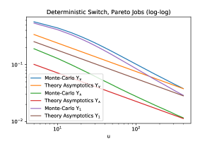
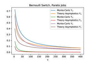
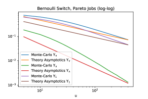
Figure 2: Simulated exceedance probabilities in the Bernoulli switch in comparison to the obtained asymptotics in natural scaling (left) and as log-log plot (right).
Here job sizes are Pareto distributed with F¯1(x)=x3/2subscript¯𝐹1𝑥superscript𝑥32\overline{F}_{1}(x)=x^{-3/2}, x1𝑥1x\geq 1, and F¯2(x)=4x2subscript¯𝐹2𝑥4superscript𝑥2\overline{F}_{2}(x)=4x^{-2}, x2𝑥2x\geq 2. Further λ1=λ2=1subscript𝜆1subscript𝜆21\lambda_{1}=\lambda_{2}=1, c1=5subscript𝑐15c_{1}=5, c2=8subscript𝑐28c_{2}=8, and b1=0.8=1b2subscript𝑏10.81subscript𝑏2b_{1}=0.8=1-b_{2}. The Bernoulli switch is characterized by p=0.4𝑝0.4p=0.4 and q=0.7𝑞0.7q=0.7. For these parameters from (5.2) we derive Υ1(u1)0.8u10.5similar-tosubscriptΥ1subscript𝑢10.8superscriptsubscript𝑢10.5\Upsilon_{1}(u_{1})\sim 0.8\cdot u_{1}^{-0.5} and Υ2(u2)0.24u20.5similar-tosubscriptΥ2subscript𝑢20.24superscriptsubscript𝑢20.5\Upsilon_{2}(u_{2})\sim 0.24\cdot u_{2}^{-0.5} such that Υ(u)0.48u1similar-tosubscriptΥ𝑢0.48superscript𝑢1\Upsilon_{\wedge}(u)\sim 0.48\cdot u^{-1} and Υ(u)1.431u0.5similar-tosubscriptΥ𝑢1.431superscript𝑢0.5\Upsilon_{\vee}(u)\sim 1.431\cdot u^{-0.5} via (5.1).
Note that a direct evaluation of the asymptotics of ΥsubscriptΥ\Upsilon_{\vee} as given in Corollary 3.9 yields the same result.
Refer to caption
Refer to caption
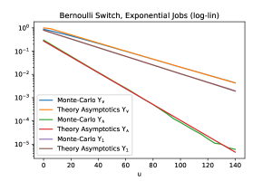
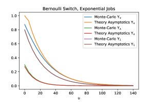
Figure 3: Simulated exceedance probabilities in the Bernoulli switch in comparison to the obtained asymptotics in natural scaling (left) and as log-linear plot (right).
Here jobs are exponentially distributed with F¯1(x)=ex/3subscript¯𝐹1𝑥superscript𝑒𝑥3\overline{F}_{1}(x)=e^{-x/3}, x0𝑥0x\geq 0, and F¯2(x)=ex/4subscript¯𝐹2𝑥superscript𝑒𝑥4\overline{F}_{2}(x)=e^{-x/4}, x0𝑥0x\geq 0. Further λ1=λ2=1subscript𝜆1subscript𝜆21\lambda_{1}=\lambda_{2}=1, c1=5subscript𝑐15c_{1}=5, c2=8subscript𝑐28c_{2}=8, and b1=0.8=1b2subscript𝑏10.81subscript𝑏2b_{1}=0.8=1-b_{2}. The Bernoulli switch is characterized by p=0.4𝑝0.4p=0.4 and q=0.7𝑞0.7q=0.7. For these parameters from (5.4) we derive κ10.054subscript𝜅10.054\kappa_{1}\approx 0.054 and κ20.178subscript𝜅20.178\kappa_{2}\approx 0.178 and (5.3) yields Υ1(u1)0.796exp(0.054u1)similar-tosubscriptΥ1subscript𝑢10.7960.054subscript𝑢1\Upsilon_{1}(u_{1})\sim 0.796\cdot\exp(-0.054u_{1}) and Υ2(u2)0.343exp(0.178u2)similar-tosubscriptΥ2subscript𝑢20.3430.178subscript𝑢2\Upsilon_{2}(u_{2})\sim 0.343\cdot\exp(-0.178u_{2}) from which Υ(u)0.273exp(0.079u)similar-tosubscriptΥ𝑢0.2730.079𝑢\Upsilon_{\wedge}(u)\sim 0.273\cdot\exp(-0.079u) and Υ(u)0.796exp(0.043u)+0.343exp(0.036u)similar-tosubscriptΥ𝑢0.7960.043𝑢0.3430.036𝑢\Upsilon_{\vee}(u)\sim 0.796\cdot\exp(-0.043u)+0.343\cdot\exp(-0.036u) via (5.1). Note that in the latter case we keep both summands, since the exponents are close together.

Indeed we obtain by direct application of Corollary 3.4 that if FI1,FI2𝒮superscriptsubscript𝐹𝐼1superscriptsubscript𝐹𝐼2𝒮F_{I}^{1},F_{I}^{2}\in\mathcal{S} (which holds in particular if X1RV(α1)subscript𝑋1RVsubscript𝛼1X_{1}\in\operatorname{RV}(\alpha_{1}), X2RV(α2)subscript𝑋2RVsubscript𝛼2X_{2}\in\operatorname{RV}(\alpha_{2}), α1,α2>1subscript𝛼1subscript𝛼21\alpha_{1},\alpha_{2}>1)

Υ1(b1u)subscriptΥ1subscript𝑏1𝑢\displaystyle\Upsilon_{1}(b_{1}u) λ1pb1uF¯1(y)dy+λ2qb1uF¯2(y)dyc1λ1p𝔼[X1]λ2q𝔼[X2],similar-toabsentsubscript𝜆1𝑝superscriptsubscriptsubscript𝑏1𝑢subscript¯𝐹1𝑦differential-d𝑦subscript𝜆2𝑞superscriptsubscriptsubscript𝑏1𝑢subscript¯𝐹2𝑦differential-d𝑦subscript𝑐1subscript𝜆1𝑝𝔼delimited-[]subscript𝑋1subscript𝜆2𝑞𝔼delimited-[]subscript𝑋2\displaystyle\sim\frac{\lambda_{1}p\int_{b_{1}u}^{\infty}\overline{F}_{1}(y)\mathop{}\!\mathrm{d}y+\lambda_{2}q\int_{b_{1}u}^{\infty}\overline{F}_{2}(y)\mathop{}\!\mathrm{d}y}{c_{1}-\lambda_{1}p\mathbb{E}[X_{1}]-\lambda_{2}q\mathbb{E}[X_{2}]}, (5.2)
andΥ2(b2u)andsubscriptΥ2subscript𝑏2𝑢\displaystyle\text{and}\quad\Upsilon_{2}(b_{2}u) λ1(1p)b2uF¯1(y)dy+λ2(1q)b2uF¯2(y)dyc1λ1(1p)𝔼[X1]λ2(1q)𝔼[X2].similar-toabsentsubscript𝜆11𝑝superscriptsubscriptsubscript𝑏2𝑢subscript¯𝐹1𝑦differential-d𝑦subscript𝜆21𝑞superscriptsubscriptsubscript𝑏2𝑢subscript¯𝐹2𝑦differential-d𝑦subscript𝑐1subscript𝜆11𝑝𝔼delimited-[]subscript𝑋1subscript𝜆21𝑞𝔼delimited-[]subscript𝑋2\displaystyle\sim\frac{\lambda_{1}(1-p)\int_{b_{2}u}^{\infty}\overline{F}_{1}(y)\mathop{}\!\mathrm{d}y+\lambda_{2}(1-q)\int_{b_{2}u}^{\infty}\overline{F}_{2}(y)\mathop{}\!\mathrm{d}y}{c_{1}-\lambda_{1}(1-p)\mathbb{E}[X_{1}]-\lambda_{2}(1-q)\mathbb{E}[X_{2}]}.

In the light-tailed case an application of Corollary 4.5 yields

Υ1(b1u)subscriptΥ1subscript𝑏1𝑢\displaystyle\Upsilon_{1}(b_{1}u) c1λ1p𝔼[X1]λ2q𝔼[X2]λ1pφX1(κ1)+λ2qφX2(κ1)eκ1b1usimilar-toabsentsubscript𝑐1subscript𝜆1𝑝𝔼delimited-[]subscript𝑋1subscript𝜆2𝑞𝔼delimited-[]subscript𝑋2subscript𝜆1𝑝superscriptsubscript𝜑subscript𝑋1subscript𝜅1subscript𝜆2𝑞superscriptsubscript𝜑subscript𝑋2subscript𝜅1superscript𝑒subscript𝜅1subscript𝑏1𝑢\displaystyle\sim\frac{c_{1}-\lambda_{1}p\mathbb{E}[X_{1}]-\lambda_{2}q\mathbb{E}[X_{2}]}{\lambda_{1}p\varphi_{X_{1}}^{\prime}(\kappa_{1})+\lambda_{2}q\varphi_{X_{2}}^{\prime}(\kappa_{1})}e^{-\kappa_{1}b_{1}u} (5.3)
andΥ2(b2u)andsubscriptΥ2subscript𝑏2𝑢\displaystyle\text{and}\quad\Upsilon_{2}(b_{2}u) c2λ1(1p)𝔼[X1]λ2(1q)𝔼[X2]λ1(1p)φX1(κ2)+λ2(1q)φX2(κ2)eκ2b2u,similar-toabsentsubscript𝑐2subscript𝜆11𝑝𝔼delimited-[]subscript𝑋1subscript𝜆21𝑞𝔼delimited-[]subscript𝑋2subscript𝜆11𝑝superscriptsubscript𝜑subscript𝑋1subscript𝜅2subscript𝜆21𝑞superscriptsubscript𝜑subscript𝑋2subscript𝜅2superscript𝑒subscript𝜅2subscript𝑏2𝑢\displaystyle\sim\frac{c_{2}-\lambda_{1}(1-p)\mathbb{E}[X_{1}]-\lambda_{2}(1-q)\mathbb{E}[X_{2}]}{\lambda_{1}(1-p)\varphi_{X_{1}}^{\prime}(\kappa_{2})+\lambda_{2}(1-q)\varphi_{X_{2}}^{\prime}(\kappa_{2})}e^{-\kappa_{2}b_{2}u},

as long as there exist κ1,κ2>0subscript𝜅1subscript𝜅20\kappa_{1},\kappa_{2}>0 such that (4.2) holds, which in the Bernoulli switch simplifies to

c1κ1subscript𝑐1subscript𝜅1\displaystyle c_{1}\kappa_{1} =λ1p(φX1(κ1)1)+λ2q(φX2(κ1)1)absentsubscript𝜆1𝑝subscript𝜑subscript𝑋1subscript𝜅11subscript𝜆2𝑞subscript𝜑subscript𝑋2subscript𝜅11\displaystyle=\lambda_{1}p(\varphi_{X_{1}}(\kappa_{1})-1)+\lambda_{2}q(\varphi_{X_{2}}(\kappa_{1})-1) (5.4)
andc2κ2andsubscript𝑐2subscript𝜅2\displaystyle\text{and}\quad c_{2}\kappa_{2} =λ1(1p)(φX1(κ2)1)+λ2(1q)(φX2(κ2)1).absentsubscript𝜆11𝑝subscript𝜑subscript𝑋1subscript𝜅21subscript𝜆21𝑞subscript𝜑subscript𝑋2subscript𝜅21\displaystyle=\lambda_{1}(1-p)(\varphi_{X_{1}}(\kappa_{2})-1)+\lambda_{2}(1-q)(\varphi_{X_{2}}(\kappa_{2})-1).

The asymptotic behavior of ΥsubscriptΥ\Upsilon_{\vee} and ΥsubscriptΥ\Upsilon_{\wedge} can now be described via (5.1).

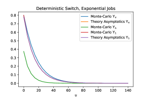
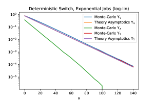
In Figures 2 and 3 we compare the asymptotics in the Bernoulli switch obtained in this way with data that has been simulated using standard Monte-Carlo techniques. As one can see in all cases the obtained asymptotics fit the data very well for u𝑢u large enough.

5.2 The deterministic switch

The deterministic switch is characterized by setting

A11subscript𝐴11\displaystyle A_{11} =d1=1A21,absentsubscript𝑑11subscript𝐴21\displaystyle=d_{1}=1-A_{21},
andA12andsubscript𝐴12\displaystyle\text{and}\quad A_{12} =d2=1A22,absentsubscript𝑑21subscript𝐴22\displaystyle=d_{2}=1-A_{22},

for some predefined constants d1,d2[0,1]subscript𝑑1subscript𝑑201d_{1},d_{2}\in[0,1].
Note that for λ2=0subscript𝜆20\lambda_{2}=0, meaning that we have only one source of claims, the corresponding dual risk model coincides with the degenerate model considered in [4, 5, 24]. Allowing two sources of claims, but setting d1(0,1)subscript𝑑101d_{1}\in(0,1), d2=1subscript𝑑21d_{2}=1 reduces our model to the setting treated in [6].
Clearly, for any choice of d1,d2subscript𝑑1subscript𝑑2d_{1},d_{2} in the deterministic switch one can easily evaluate the asymptotics of the exceedance probabilities as given in Corollaries 3.4 , 3.9, and 4.5 since all appearing expectations disappear.
Refer to caption
Refer to caption
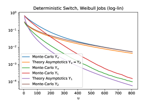
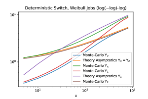
Figure 4: Simulated exceedance probabilities in the deterministic switch in comparison to the obtained asymptotics as log-lin plot (left) and log(-log)-log plot (right), meaning the y𝑦y-axis is scaled as log(log(y))𝑦\log(-\log(y)), while the x𝑥x-axis is scaled as log(x)𝑥\log(x). This particular scaling of the axes is chosen in order to get straight lines of ascent γ1superscript𝛾1\gamma^{-1}, for functions of the type exγsuperscript𝑒𝛾𝑥e^{-\sqrt[\gamma]{x}}.
Job sizes are Weibull distributed with F¯1(x)=1exp((2x)13)subscript¯𝐹1𝑥1superscript2𝑥13\overline{F}_{1}(x)=1-\exp((2x)^{\frac{1}{3}}), x0𝑥0x\geq 0, and F¯2(x)=1exp((x/2)12)subscript¯𝐹2𝑥1superscript𝑥212\overline{F}_{2}(x)=1-\exp((x/2)^{\frac{1}{2}}), x0𝑥0x\geq 0. Further λ1=λ2=1subscript𝜆1subscript𝜆21\lambda_{1}=\lambda_{2}=1, c1=5subscript𝑐15c_{1}=5, c2=8subscript𝑐28c_{2}=8, and b1=0.8=1b2subscript𝑏10.81subscript𝑏2b_{1}=0.8=1-b_{2}. The deterministic switch is characterized by d1=0.4subscript𝑑10.4d_{1}=0.4 and d2=0.7subscript𝑑20.7d_{2}=0.7. For these parameters from Corollary 3.4 we derive Υ2(b2u)Υ(u)(0.1374u23+0.31449u13+0.36)exp(0.87358u13)similar-tosubscriptΥ2subscript𝑏2𝑢subscriptΥ𝑢similar-to0.1374superscript𝑢230.31449superscript𝑢130.360.87358superscript𝑢13\Upsilon_{2}(b_{2}u)\sim\Upsilon_{\vee}(u)\sim(0.1374\cdot u^{\frac{2}{3}}+0.31449\cdot u^{\frac{1}{3}}+0.36)\cdot\exp(-0.87358\cdot u^{\frac{1}{3}}), and Υ1(b1u)(1.51191u23+1.90488u13+1.2)exp(1.58740u13)similar-tosubscriptΥ1subscript𝑏1𝑢1.51191superscript𝑢231.90488superscript𝑢131.21.58740superscript𝑢13\Upsilon_{1}(b_{1}u)\sim(1.51191\cdot u^{\frac{2}{3}}+1.90488\cdot u^{\frac{1}{3}}+1.2)\cdot\exp(-1.58740\cdot u^{\frac{1}{3}}), while for ΥsubscriptΥ\Upsilon_{\wedge} no asymptotics are given as (3.9) fails.
Refer to caption
Refer to caption
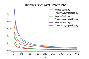
Figure 5: Simulated exceedance probabilities in the deterministic switch in comparison to the obtained asymptotics in natural scaling (left) and as log-log plot (right).
Here - as in Figure 2 - job sizes are Pareto distributed with F¯1(x)=x3/2subscript¯𝐹1𝑥superscript𝑥32\overline{F}_{1}(x)=x^{-3/2}, x1𝑥1x\geq 1, and F¯2(x)=4x2subscript¯𝐹2𝑥4superscript𝑥2\overline{F}_{2}(x)=4x^{-2}, x2𝑥2x\geq 2. Further λ1=λ2=1subscript𝜆1subscript𝜆21\lambda_{1}=\lambda_{2}=1, c1=5subscript𝑐15c_{1}=5, c2=8subscript𝑐28c_{2}=8, and b1=0.8=1b2subscript𝑏10.81subscript𝑏2b_{1}=0.8=1-b_{2}. The deterministic switch is characterized by d1=0.4subscript𝑑10.4d_{1}=0.4 and d2=0.7subscript𝑑20.7d_{2}=0.7. For these parameters from Corollary 3.9 we derive Υ1(u1)0.506u10.5similar-tosubscriptΥ1subscript𝑢10.506superscriptsubscript𝑢10.5\Upsilon_{1}(u_{1})\sim 0.506\cdot u_{1}^{-0.5}, and Υ2(u2)0.186u20.5similar-tosubscriptΥ2subscript𝑢20.186superscriptsubscript𝑢20.5\Upsilon_{2}(u_{2})\sim 0.186\cdot u_{2}^{-0.5}, while Υ(u)0.756u0.5similar-tosubscriptΥ𝑢0.756superscript𝑢0.5\Upsilon_{\vee}(u)\sim 0.756\cdot u^{-0.5}, and Υ(u)0.226u0.5similar-tosubscriptΥ𝑢0.226superscript𝑢0.5\Upsilon_{\wedge}(u)\sim 0.226\cdot u^{-0.5}.
Refer to caption
Refer to caption
Figure 6: Simulated exceedance probabilities in the deterministic switch in comparison to the obtained asymptotics in natural scaling (left) and as log-linear plot (right).
Here jobs are - as in Figure 3 - exponentially distributed with F¯1(x)=ex/3subscript¯𝐹1𝑥superscript𝑒𝑥3\overline{F}_{1}(x)=e^{-x/3}, x0𝑥0x\geq 0, and F¯2(x)=ex/4subscript¯𝐹2𝑥superscript𝑒𝑥4\overline{F}_{2}(x)=e^{-x/4}, x0𝑥0x\geq 0. Further λ1=λ2=1subscript𝜆1subscript𝜆21\lambda_{1}=\lambda_{2}=1, c1=5subscript𝑐15c_{1}=5, c2=8subscript𝑐28c_{2}=8, and b1=0.8=1b2subscript𝑏10.81subscript𝑏2b_{1}=0.8=1-b_{2}. The deterministic switch is characterized by d1=0.4subscript𝑑10.4d_{1}=0.4 and d2=0.7subscript𝑑20.7d_{2}=0.7. For these parameters from (4.2) we obtain κ10.084subscript𝜅10.084\kappa_{1}\approx 0.084 and κ20.383subscript𝜅20.383\kappa_{2}\approx 0.383, which yield Υ1(u1)0.78exp(0.084u1)similar-tosubscriptΥ1subscript𝑢10.780.084subscript𝑢1\Upsilon_{1}(u_{1})\sim 0.78\cdot\exp(-0.084u_{1}) and Υ2(u2)0.341exp(0.383u2)similar-tosubscriptΥ2subscript𝑢20.3410.383subscript𝑢2\Upsilon_{2}(u_{2})\sim 0.341\cdot\exp(-0.383u_{2}), while Υ(u)0.78exp(0.067u)+0.341exp(0.077u)similar-tosubscriptΥ𝑢0.780.067𝑢0.3410.077𝑢\Upsilon_{\vee}(u)\sim 0.78\cdot\exp(-0.067u)+0.341\cdot\exp(-0.077u) and Υ(u)=o(exp(0.067u))subscriptΥ𝑢𝑜0.067𝑢\Upsilon_{\wedge}(u)=o(\exp(-0.067u)) by Corollary 3.9.

In Figures 4, 5, and 6 we compare the asymptotics and bounds in the deterministic switch obtained in this way with data that has been simulated using standard Monte-Carlo techniques. Again simulations and theoretical asymptotics fit well in all cases. Note that in contrast to the cases with lighter tails, in the purely subexponential case depicted in Figure 4 we observe that Υ1subscriptΥ1\Upsilon_{1} is close to ΥsubscriptΥ\Upsilon_{\vee} for small u𝑢u, but close to ΥsubscriptΥ\Upsilon_{\wedge} for large u𝑢u. This can be interpreted as follows. While for small u𝑢u the net working speed cisuperscriptsubscript𝑐𝑖c_{i}^{*} determines the exceedance probabilities, for large u𝑢u this becomes less relevant and the workload exceedance is mainly influenced by the heavyness of the tails.

Example 5.1.

Consider a deterministic switch with d1(0,1)subscript𝑑101d_{1}\in(0,1) and λ2=0subscript𝜆20\lambda_{2}=0, i.e. there is only one source of jobs and the jobs are distributed deterministically to the two servers with proportions d1subscript𝑑1d_{1} and 1d11subscript𝑑11-d_{1}, and assume that b1d1<b21d1subscript𝑏1subscript𝑑1subscript𝑏21subscript𝑑1\tfrac{b_{1}}{d_{1}}<\tfrac{b_{2}}{1-d_{1}}, such that the resulting dual risk model properly rescaled coincides with the degenerate model studied in [4, 5, 24]. Then, applying Theorem 3.1 in this setting reproduces the tail behavior of the probability of ruin of at least one component stated in [24, Cor. 2.2]. Interestingly, also the ruin probability of both insurance companies one derives in this case from Proposition 3.3 coincides with the asymptotics provided in [24, Eq. (2.9)], although the latter corresponds to simultaneous ruin. This suggests that in this special setting the ruin probability of both components and the simultaneous ruin probability of both components are asymptotically equivalent.

5.3 A comparison of different switches

In this section we aim to compare the two above special cases of the Bernoulli switch and the deterministic switch with a non-trivial random switch, which we chose to be a Beta switch characterized by setting

A11subscript𝐴11\displaystyle A_{11} =1A21Beta(β1,γ1),absent1subscript𝐴21similar-toBetasubscript𝛽1subscript𝛾1\displaystyle=1-A_{21}\sim\operatorname{Beta}(\beta_{1},\gamma_{1}),
andA12andsubscript𝐴12\displaystyle\text{and}\quad A_{12} =1A22Beta(β2,γ2)absent1subscript𝐴22similar-toBetasubscript𝛽2subscript𝛾2\displaystyle=1-A_{22}\sim\operatorname{Beta}(\beta_{2},\gamma_{2})

for some constants β1,β2,γ1,γ2>0subscript𝛽1subscript𝛽2subscript𝛾1subscript𝛾20\beta_{1},\beta_{2},\gamma_{1},\gamma_{2}>0, where Beta(β,γ)Beta𝛽𝛾\text{Beta}(\beta,\gamma) is the Beta distribution with density Γ(β+γ)Γ(β)Γ(γ)xβ1(1x)γ1Γ𝛽𝛾Γ𝛽Γ𝛾superscript𝑥𝛽1superscript1𝑥𝛾1\frac{\Gamma(\beta+\gamma)}{\Gamma(\beta)\Gamma(\gamma)}x^{\beta-1}(1-x)^{\gamma-1}, x[0,1]𝑥01x\in[0,1].
To keep all examples comparable, we fix λ1subscript𝜆1\lambda_{1}, λ2subscript𝜆2\lambda_{2}, 𝔼[X1]𝔼delimited-[]subscript𝑋1\mathbb{E}[X_{1}], 𝔼[X2]𝔼delimited-[]subscript𝑋2\mathbb{E}[X_{2}], 𝔼[A11]𝔼delimited-[]subscript𝐴11\mathbb{E}[A_{11}] and 𝔼[A12]𝔼delimited-[]subscript𝐴12\mathbb{E}[A_{12}] such that the scenarios only differ in the behavior of the switch and the job sizes. Figure 7 shows the approximate exceedance probabilities obtained by Monte Carlo simulation for the Bernoulli switch, the deterministic switch und two different Beta switches.
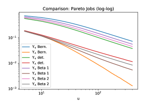
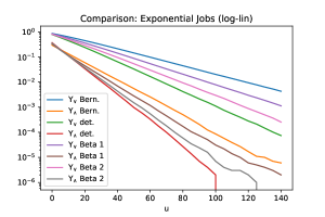
Refer to caption
Refer to caption
Figure 7: Simulated exceedance probabilities for different switches with heavy-tailed (left, log-log plot) and light-tailed (right, log-linear plot) job sizes.
Throughout λ1=λ2=1subscript𝜆1subscript𝜆21\lambda_{1}=\lambda_{2}=1, c1=5subscript𝑐15c_{1}=5, c2=8subscript𝑐28c_{2}=8, and b1=0.8=1b2subscript𝑏10.81subscript𝑏2b_{1}=0.8=1-b_{2}. On the left - as in Figures 2 and 5 - job sizes are Pareto distributed with F¯1(x)=x3/2subscript¯𝐹1𝑥superscript𝑥32\overline{F}_{1}(x)=x^{-3/2}, x1𝑥1x\geq 1, and F¯2(x)=4x2subscript¯𝐹2𝑥4superscript𝑥2\overline{F}_{2}(x)=4x^{-2}, x2𝑥2x\geq 2. On the right jobs are - as in Figures 3 and 6 - exponentially distributed with F¯1(x)=ex/3subscript¯𝐹1𝑥superscript𝑒𝑥3\overline{F}_{1}(x)=e^{-x/3}, x0𝑥0x\geq 0, and F¯2(x)=ex/4subscript¯𝐹2𝑥superscript𝑒𝑥4\overline{F}_{2}(x)=e^{-x/4}, x0𝑥0x\geq 0. The Bernoulli switch is characterized by p=0.4𝑝0.4p=0.4 and q=0.7𝑞0.7q=0.7, the deterministic switch is characterized by d1=0.4subscript𝑑10.4d_{1}=0.4 and d2=0.7subscript𝑑20.7d_{2}=0.7, the Beta switch 1 is characterized by A11=1A21Beta(0.4,0.6)subscript𝐴111subscript𝐴21similar-toBeta0.40.6A_{11}=1-A_{21}\sim\operatorname{Beta}(0.4,0.6) and A12=1A22Beta(0.7,0.3)subscript𝐴121subscript𝐴22similar-toBeta0.70.3A_{12}=1-A_{22}\sim\operatorname{Beta}(0.7,0.3), and the Beta switch 2 is characterized by A11=1A21Beta(1.5,2.25)subscript𝐴111subscript𝐴21similar-toBeta1.52.25A_{11}=1-A_{21}\sim\operatorname{Beta}(1.5,2.25) and A12=1A22Beta(3,9/7)subscript𝐴121subscript𝐴22similar-toBeta397A_{12}=1-A_{22}\sim\operatorname{Beta}(3,9/7).

As we can see, in the regularly varying case the probability that at least one of the workloads exceeds the barrier ΥsubscriptΥ\Upsilon_{\vee} tends to zero with the same index of regular variation for all choices of the random switch. In case of the probability that both components exceed their barrier ΥsubscriptΥ\Upsilon_{\wedge}, the Bernoulli switch yields a faster decay due to the independence of the two workload processes in this model.
Further, the figure indicates the intuitive behavior: The more correlated the co-ordinates of the workload process are, the closer together are ΥsubscriptΥ\Upsilon_{\vee} and ΥsubscriptΥ\Upsilon_{\wedge}. This leads to a trade-off between the two probabilities: Changing the switch towards reducing one probability raises the other and the Beta switches may serve here as a compromise to control both probabilities.

In the light-tailed case the trade-off between ΥsubscriptΥ\Upsilon_{\vee} and ΥsubscriptΥ\Upsilon_{\wedge} can not be observed. Quite the contrary, the more correlated the co-ordinates of the workload process are, the lower tend to be the exceedance probabilities. Hence in this case the Bernoulli switch yields the highest exceedance probabilities, while the deterministic switch obtains the best results.

Thus, for keeping ΥsubscriptΥ\Upsilon_{\vee} small, in general the simple deterministic switch yields good results. On the contrary, if one is interested to keep ΥsubscriptΥ\Upsilon_{\wedge} small, the tail-behavior of the appearing jobs is crucial for the choice of the optimal switch. Here again Beta switches or other non-trivial random switches may serve as a compromise in situations where the tail-behavior of the appearing jobs is unknown.

6 Proofs

6.1 Proofs for Section 3.1

To prove the asymptotic result for the ruin probability ΨsubscriptΨ\Psi_{\vee} as given in Theorem 3.1 we need some preliminary definitions and results.

Let

:={M2:M open, increasing, Mc convex, 𝟎M¯}assignconditional-set𝑀superscript2𝑀 open, increasing, superscript𝑀𝑐 convex, 0¯𝑀\mathcal{R}:=\{M\subset\mathbb{R}^{2}:\leavevmode\nobreak\ M\text{ open, increasing, }M^{c}\text{ convex, }\mathbf{0}\notin\overline{M}\}

be a family of open sets, where increasing means, that for each 𝐱M𝐱𝑀\mathbf{x}\in M and 𝐝𝟎𝐝0\mathbf{d}\geq\mathbf{0} we have 𝐱+𝐝M𝐱𝐝𝑀\mathbf{x}+\mathbf{d}\in M. Let Π(dx)Πd𝑥\Pi(\mathop{}\!\mathrm{d}x) be a probability measure on 02subscriptsuperscript2absent0\mathbb{R}^{2}_{\geq 0}. For M𝑀M\in\mathcal{R} we define a cdf on [0,)0[0,\infty) by setting

FM(t):=1Π(tM),t0.formulae-sequenceassignsubscript𝐹𝑀𝑡1Π𝑡𝑀𝑡0F_{M}(t):=1-\Pi(tM),\leavevmode\nobreak\ t\geq 0.

Then, following [36, Def. 4.6], if FM𝒮subscript𝐹𝑀𝒮F_{M}\in\mathcal{S} we say that Π𝒮MΠsubscript𝒮𝑀\Pi\in\mathcal{S}_{M}. Furthermore ΠΠ\Pi is multivariate subexponential, if Π𝒮:=M𝒮MΠsubscript𝒮assignsubscript𝑀subscript𝒮𝑀\Pi\in\mathcal{S}_{\mathcal{R}}:=\bigcap_{M\in\mathcal{R}}\mathcal{S}_{M}.
Throughout this section we consider the specific sets

L:=2\𝟎2andM:=𝐛L.formulae-sequenceassign𝐿\superscript2subscriptsuperscript2absent0andassign𝑀𝐛𝐿L:=\mathbb{R}^{2}\backslash\mathbb{R}^{2}_{\geq\mathbf{0}}\qquad\text{and}\qquad M:=\mathbf{b}-L. (6.1)

Then clearly M𝑀M\in\mathcal{R} and by [36, Rem. 4.1] also uM𝑢𝑀uM\in\mathcal{R} for all u>0𝑢0u>0.
Moreover, we specify ΠΠ\Pi to be the probability measure of the claims 𝐀𝐁𝐗𝐀𝐁𝐗\mathbf{A}\mathbf{B}\mathbf{X} in the dual risk model described in Section 2.2. Then we can prove some basic relationships in the upcoming lemma.

Lemma 6.1.

Consider the probability measure ΠΠ\Pi as just defined, the set M𝑀M as in (6.1), and the constant θ𝜃\theta given in (3.2). Then

Π(uM+v𝐜)Π𝑢𝑀𝑣superscript𝐜\displaystyle\Pi(uM+v\mathbf{c}^{\ast}) =g(u,v),absent𝑔𝑢𝑣\displaystyle=g(u,v),

with g(u,v)𝑔𝑢𝑣g(u,v) defined in (3.1), and

Π(02+v𝐜)=λ1λ𝔼[F¯1(vmax{c1A11,c2A21})]+λ2λ𝔼[F¯2(vmax{c1A12,c2A22})],Πsuperscriptsubscriptabsent02𝑣superscript𝐜subscript𝜆1𝜆𝔼delimited-[]subscript¯𝐹1𝑣superscriptsubscript𝑐1subscript𝐴11superscriptsubscript𝑐2subscript𝐴21subscript𝜆2𝜆𝔼delimited-[]subscript¯𝐹2𝑣superscriptsubscript𝑐1subscript𝐴12superscriptsubscript𝑐2subscript𝐴22\displaystyle\Pi(\mathbb{R}_{\geq 0}^{2}+v\mathbf{c}^{\ast})=\frac{\lambda_{1}}{\lambda}\cdot\mathbb{E}\left[\overline{F}_{1}\left(v\cdot\max\left\{\tfrac{c_{1}^{\ast}}{A_{11}},\tfrac{c_{2}^{\ast}}{A_{21}}\right\}\right)\right]+\frac{\lambda_{2}}{\lambda}\cdot\mathbb{E}\left[\overline{F}_{2}\left(v\cdot\max\left\{\tfrac{c_{1}^{\ast}}{A_{12}},\tfrac{c_{2}^{\ast}}{A_{22}}\right\}\right)\right],

for all u>0,v0formulae-sequence𝑢0𝑣0u>0,\leavevmode\nobreak\ v\geq 0 and 𝐜>𝟎2superscript𝐜subscriptsuperscript2absent0\mathbf{c}^{\ast}\in\mathbb{R}^{2}_{>\mathbf{0}}. Moreover

θ=0Π(02+v𝐜)dv<.𝜃superscriptsubscript0Πsuperscriptsubscriptabsent02𝑣superscript𝐜differential-d𝑣\theta=\int_{0}^{\infty}\Pi\left(\mathbb{R}_{\geq 0}^{2}+v\mathbf{c}^{*}\right)\mathop{}\!\mathrm{d}v<\infty.
Proof.

By definition of M𝑀M, L𝐿L and ΠΠ\Pi and conditioning on 𝐁𝐁\mathbf{B}

Π(uM+v𝐜)Π𝑢𝑀𝑣superscript𝐜\displaystyle\Pi(uM+v\mathbf{c}^{*}) =(𝐀𝐁𝐗u𝐛+v𝐜uL)=(𝐀𝐁𝐗u𝐛+v𝐜+2\𝟎2)absent𝐀𝐁𝐗𝑢𝐛𝑣superscript𝐜𝑢𝐿𝐀𝐁𝐗𝑢𝐛𝑣superscript𝐜\superscript2subscriptsuperscript2absent0\displaystyle=\mathbb{P}\left(\mathbf{A}\mathbf{B}\mathbf{X}\in u\mathbf{b}+v\mathbf{c}^{*}-uL\right)=\mathbb{P}\left(\mathbf{A}\mathbf{B}\mathbf{X}\in u\mathbf{b}+v\mathbf{c}^{*}+\mathbb{R}^{2}\backslash\mathbb{R}^{2}_{\leq\mathbf{0}}\right)
=λ1λ((A11A21)X1u𝐛+v𝐜+2\𝟎2)absentsubscript𝜆1𝜆matrixsubscript𝐴11subscript𝐴21subscript𝑋1𝑢𝐛𝑣superscript𝐜\superscript2subscriptsuperscript2absent0\displaystyle=\frac{\lambda_{1}}{\lambda}\mathbb{P}\left(\begin{pmatrix}A_{11}\\ A_{21}\end{pmatrix}X_{1}\in u\mathbf{b}+v\mathbf{c}^{*}+\mathbb{R}^{2}\backslash\mathbb{R}^{2}_{\leq\mathbf{0}}\right)
+λ2λ((A12A22)X2u𝐛+v𝐜+2\𝟎2),subscript𝜆2𝜆matrixsubscript𝐴12subscript𝐴22subscript𝑋2𝑢𝐛𝑣superscript𝐜\superscript2subscriptsuperscript2absent0\displaystyle\qquad+\frac{\lambda_{2}}{\lambda}\mathbb{P}\left(\begin{pmatrix}A_{12}\\ A_{22}\end{pmatrix}X_{2}\in u\mathbf{b}+v\mathbf{c}^{*}+\mathbb{R}^{2}\backslash\mathbb{R}^{2}_{\leq\mathbf{0}}\right),

where for j=1,2𝑗12j=1,2

((A1jA2j)Xju𝐛+v𝐜+d\𝟎d)matrixsubscript𝐴1𝑗subscript𝐴2𝑗subscript𝑋𝑗𝑢𝐛𝑣superscript𝐜\superscript𝑑subscriptsuperscript𝑑absent0\displaystyle\mathbb{P}\bigg{(}\begin{pmatrix}A_{1j}\\ A_{2j}\end{pmatrix}X_{j}\in u\mathbf{b}+v\mathbf{c}^{*}+\mathbb{R}^{d}\backslash\mathbb{R}^{d}_{\leq\mathbf{0}}\bigg{)} =((A1jXj>ub1+vc1) or (A2jXj>ub2+vc2))absentsubscript𝐴1𝑗subscript𝑋𝑗𝑢subscript𝑏1𝑣superscriptsubscript𝑐1 or subscript𝐴2𝑗subscript𝑋𝑗𝑢subscript𝑏2𝑣superscriptsubscript𝑐2\displaystyle=\mathbb{P}\left((A_{1j}X_{j}>ub_{1}+vc_{1}^{*})\text{ or }(A_{2j}X_{j}>ub_{2}+vc_{2}^{*})\right)
=(Xj>min{ub1+vc1A1j,ub2+vc2A2j})absentsubscript𝑋𝑗𝑢subscript𝑏1𝑣superscriptsubscript𝑐1subscript𝐴1𝑗𝑢subscript𝑏2𝑣superscriptsubscript𝑐2subscript𝐴2𝑗\displaystyle=\mathbb{P}\left(X_{j}>\min\left\{\tfrac{ub_{1}+vc_{1}^{*}}{A_{1j}},\tfrac{ub_{2}+vc_{2}^{*}}{A_{2j}}\right\}\right)
=𝔼[F¯j(min{ub1+vc1A1j,ub2+vc2A2j})],absent𝔼delimited-[]subscript¯𝐹𝑗𝑢subscript𝑏1𝑣superscriptsubscript𝑐1subscript𝐴1𝑗𝑢subscript𝑏2𝑣superscriptsubscript𝑐2subscript𝐴2𝑗\displaystyle=\mathbb{E}\left[\overline{F}_{j}\left(\min\left\{\tfrac{ub_{1}+vc_{1}^{*}}{A_{1j}},\tfrac{ub_{2}+vc_{2}^{*}}{A_{2j}}\right\}\right)\right],

which proves the first equation. The second equation follows by an analogue computation.
Lastly, using the obtained expression for Π(02+v𝐜)Πsuperscriptsubscriptabsent02𝑣superscript𝐜\Pi(\mathbb{R}_{\geq 0}^{2}+v\mathbf{c}^{\ast}) we may compute using Tonelli’s theorem

0Π(02+v𝐜)𝑑vsuperscriptsubscript0Πsuperscriptsubscriptabsent02𝑣superscript𝐜differential-d𝑣\displaystyle\int_{0}^{\infty}\Pi(\mathbb{R}_{\geq 0}^{2}+v\cdot\mathbf{c}^{\ast})dv
=λ1λ𝔼[0F¯1(vmax{c1A11,c2A21})dv]+λ2λ𝔼[0F¯2(vmax{c1A12,c2A22})dv],absentsubscript𝜆1𝜆𝔼delimited-[]superscriptsubscript0subscript¯𝐹1𝑣superscriptsubscript𝑐1subscript𝐴11superscriptsubscript𝑐2subscript𝐴21differential-d𝑣subscript𝜆2𝜆𝔼delimited-[]superscriptsubscript0subscript¯𝐹2𝑣superscriptsubscript𝑐1subscript𝐴12superscriptsubscript𝑐2subscript𝐴22differential-d𝑣\displaystyle=\frac{\lambda_{1}}{\lambda}\mathbb{E}\left[\int_{0}^{\infty}\overline{F}_{1}\left(v\cdot\max\left\{\tfrac{c_{1}^{*}}{A_{11}},\tfrac{c_{2}^{*}}{A_{21}}\right\}\right)\mathop{}\!\mathrm{d}v\right]+\frac{\lambda_{2}}{\lambda}\mathbb{E}\left[\int_{0}^{\infty}\overline{F}_{2}\left(v\cdot\max\left\{\tfrac{c_{1}^{*}}{A_{12}},\tfrac{c_{2}^{*}}{A_{22}}\right\}\right)\mathop{}\!\mathrm{d}v\right],

where for j=1,2𝑗12j=1,2

𝔼[0F¯j(vmax{c1A1j,c2A2j})dv]𝔼delimited-[]superscriptsubscript0subscript¯𝐹𝑗𝑣superscriptsubscript𝑐1subscript𝐴1𝑗superscriptsubscript𝑐2subscript𝐴2𝑗differential-d𝑣\displaystyle\mathbb{E}\left[\int_{0}^{\infty}\overline{F}_{j}\left(v\cdot\max\left\{\tfrac{c_{1}^{*}}{A_{1j}},\tfrac{c_{2}^{*}}{A_{2j}}\right\}\right)\mathop{}\!\mathrm{d}v\right] =𝔼[(max{c1A1j,c2A2j})10F¯1(y)dy]absent𝔼delimited-[]superscriptsuperscriptsubscript𝑐1subscript𝐴1𝑗superscriptsubscript𝑐2subscript𝐴2𝑗1superscriptsubscript0subscript¯𝐹1𝑦differential-d𝑦\displaystyle=\mathbb{E}\left[\left(\max\left\{\tfrac{c_{1}^{*}}{A_{1j}},\tfrac{c_{2}^{*}}{A_{2j}}\right\}\right)^{-1}\int_{0}^{\infty}\overline{F}_{1}\left(y\right)\mathop{}\!\mathrm{d}y\right]
=𝔼[min{A1jc1,A2jc2}]𝔼[Xj].absent𝔼delimited-[]subscript𝐴1𝑗superscriptsubscript𝑐1subscript𝐴2𝑗superscriptsubscript𝑐2𝔼delimited-[]subscript𝑋𝑗\displaystyle=\mathbb{E}\left[\min\left\{\tfrac{A_{1j}}{c_{1}^{*}},\tfrac{A_{2j}}{c_{2}^{*}}\right\}\right]\mathbb{E}[X_{j}].

This proves 0Π(02+v𝐜)𝑑v=θsuperscriptsubscript0Πsuperscriptsubscriptabsent02𝑣superscript𝐜differential-d𝑣𝜃\int_{0}^{\infty}\Pi(\mathbb{R}_{\geq 0}^{2}+v\mathbf{c}^{\ast})dv=\theta. Moreover we note that the finite mean of the claim sizes Xjsubscript𝑋𝑗X_{j} implies finiteness of 0Π(02+v𝐜)dvsuperscriptsubscript0Πsuperscriptsubscriptabsent02𝑣superscript𝐜differential-d𝑣\int_{0}^{\infty}\Pi\left(\mathbb{R}_{\geq 0}^{2}+v\mathbf{c}^{*}\right)\mathop{}\!\mathrm{d}v. ∎

Proof of Theorem 3.1.

Recall the definition of the set L𝐿L in (6.1) and note that obviously L𝐿L satisfies [36, Assumption 5.1]. Furthermore note that u𝐛𝐑(t)L𝑢𝐛𝐑𝑡𝐿u\mathbf{b}-\mathbf{R}(t)\in L if and only if maxi=1,2(Ri(t)ubi)>0subscript𝑖12subscript𝑅𝑖𝑡𝑢subscript𝑏𝑖0\max_{i=1,2}(R_{i}(t)-ub_{i})>0, which immediately implies that

Ψ(u)subscriptΨ𝑢\displaystyle\Psi_{\vee}(u) =(u𝐛𝐑(t)L for some t0)absent𝑢𝐛𝐑𝑡𝐿 for some 𝑡0\displaystyle=\mathbb{P}(u\mathbf{b}-\mathbf{R}(t)\in L\text{ for some }t\geq 0)
=(𝐑(t)uM for some t0),u>0.formulae-sequenceabsent𝐑𝑡𝑢𝑀 for some 𝑡0𝑢0\displaystyle=\mathbb{P}(\mathbf{R}(t)\in uM\text{ for some }t\geq 0),\quad u>0.

Thus, by [36, Thm. 5.2] we obtain

Ψ(u)0Π(uM+v𝐜)dv,similar-tosubscriptΨ𝑢superscriptsubscript0Π𝑢𝑀𝑣superscript𝐜differential-d𝑣\Psi_{\vee}(u)\sim\int_{0}^{\infty}\Pi(uM+v\mathbf{c^{*}})\mathop{}\!\mathrm{d}v, (6.2)

as soon as we can guarantee that the probability measure on 2superscript2\mathbb{R}^{2} defined by

ΠI(D)=θ10Π(D+v𝐜)dv,for any Borel set D02,formulae-sequencesuperscriptΠ𝐼𝐷superscript𝜃1superscriptsubscript0Π𝐷𝑣superscript𝐜differential-d𝑣for any Borel set 𝐷subscriptsuperscript2absent0\Pi^{I}(D)=\theta^{-1}\int_{0}^{\infty}\Pi(D+v\mathbf{c}^{\ast})\mathop{}\!\mathrm{d}v,\quad\text{for any Borel set }D\subset\mathbb{R}^{2}_{\geq 0},

and ΠI(202)=0superscriptΠ𝐼superscript2superscriptsubscriptabsent020\Pi^{I}(\mathbb{R}^{2}\setminus\mathbb{R}_{\geq 0}^{2})=0, is in 𝒮Msubscript𝒮𝑀\mathcal{S}_{M}. This however is by definition equivalent to the assumption that the cdf FM(u)=1ΠI(uM)subscript𝐹𝑀𝑢1superscriptΠ𝐼𝑢𝑀F_{M}(u)=1-\Pi^{I}(uM), u0𝑢0u\geq 0, is in 𝒮𝒮\mathcal{S}. Since by Lemma 6.1 FM(u)=Fsubexp(u)subscript𝐹𝑀𝑢subscript𝐹subexp𝑢F_{M}(u)=F_{\text{subexp}}(u) with Fsubexpsubscript𝐹subexpF_{\text{subexp}} as given in (3.3), this is assumed in the theorem. Lastly, observe that the right hand side of (6.2) equals 0g(u,v)dvsuperscriptsubscript0𝑔𝑢𝑣differential-d𝑣\int_{0}^{\infty}g(u,v)\mathop{}\!\mathrm{d}v as shown in Lemma 6.1. ∎

Remark 6.2.

Naively one could guess that subexponentiality of the claims X1subscript𝑋1X_{1} and X2subscript𝑋2X_{2} should be enough to obtain subexponentiality of at least ΠΠ\Pi. However, as noted in [36, Remark 4.9] this is not true in general, because random mixing of two subexponential distributions (as done by our matrix 𝐁𝐁\mathbf{B}) leads to a subexponential distribution if and only if the sum of the mixed distributions is subexponential. This again is not true in general.

Proof of Lemma 3.2.

Fix i{1,2}𝑖12i\in\{1,2\} and assume that (Ai1+Ai2=0)<1.subscript𝐴𝑖1subscript𝐴𝑖201\mathbb{P}(A_{i1}+A_{i2}=0)<1. Otherwise Ri(t)subscript𝑅𝑖𝑡R_{i}(t) is monotonely decreasing, Ψi(u)=0subscriptΨ𝑖𝑢0\Psi_{i}(u)=0, and the statement is proven. Note that by definition

Ψi(u)subscriptΨ𝑖𝑢\displaystyle\Psi_{i}(u) =(k=1N(t)((B11)k(Ai1)kX1,k+(B22)k(Ai2)kX2,k)tci>u for some t>0)absentsuperscriptsubscript𝑘1𝑁𝑡subscriptsubscript𝐵11𝑘subscriptsubscript𝐴𝑖1𝑘subscript𝑋1𝑘subscriptsubscript𝐵22𝑘subscriptsubscript𝐴𝑖2𝑘subscript𝑋2𝑘𝑡subscript𝑐𝑖𝑢 for some 𝑡0\displaystyle=\mathbb{P}\Bigg{(}\sum_{k=1}^{N(t)}\big{(}(B_{11})_{k}(A_{i1})_{k}X_{1,k}+(B_{22})_{k}(A_{i2})_{k}X_{2,k}\big{)}-tc_{i}>u\text{ for some }t>0\Bigg{)}
=:(k=1N(t)Yi,ktci>u for some t>0),i=1,2,\displaystyle=:\mathbb{P}\Bigg{(}\sum_{k=1}^{N(t)}Y_{i,k}-tc_{i}>u\text{ for some }t>0\Bigg{)},\quad i=1,2,

where the random variables {Yi,k,k}subscript𝑌𝑖𝑘𝑘\{Y_{i,k},k\in\mathbb{N}\} are i.i.d. copies of two generic random variables Yisubscript𝑌𝑖Y_{i}, i=1,2𝑖12i=1,2. The corresponding integrated tail function is defined as

FIYi(x):=𝔼[Yi]10x(Yi>y)dy,x0.formulae-sequenceassignsubscriptsuperscript𝐹subscript𝑌𝑖𝐼𝑥𝔼superscriptdelimited-[]subscript𝑌𝑖1superscriptsubscript0𝑥subscript𝑌𝑖𝑦differential-d𝑦𝑥0F^{Y_{i}}_{I}(x):=\mathbb{E}[Y_{i}]^{-1}\int_{0}^{x}\mathbb{P}(Y_{i}>y)\mathop{}\!\mathrm{d}y,\quad x\geq 0.

From [3, Thm. X.2.1] we obtain that if FIYi𝒮subscriptsuperscript𝐹subscript𝑌𝑖𝐼𝒮F^{Y_{i}}_{I}\in\mathcal{S}

limuΨi(u)FYi¯I(u)=λ𝔼[Yi]ciλ𝔼[Yi],subscript𝑢subscriptΨ𝑖𝑢subscript¯superscript𝐹subscript𝑌𝑖𝐼𝑢𝜆𝔼delimited-[]subscript𝑌𝑖subscript𝑐𝑖𝜆𝔼delimited-[]subscript𝑌𝑖\lim_{u\to\infty}\frac{\Psi_{i}(u)}{\overline{F^{Y_{i}}}_{I}(u)}=\frac{\lambda\mathbb{E}[Y_{i}]}{c_{i}-\lambda\mathbb{E}[Y_{i}]}, (6.3)

where

𝔼[Yi]=λ1λ𝔼[Ai1]𝔼[X1]+λ2λ𝔼[Ai2]𝔼[X2],𝔼delimited-[]subscript𝑌𝑖subscript𝜆1𝜆𝔼delimited-[]subscript𝐴𝑖1𝔼delimited-[]subscript𝑋1subscript𝜆2𝜆𝔼delimited-[]subscript𝐴𝑖2𝔼delimited-[]subscript𝑋2\mathbb{E}[Y_{i}]=\frac{\lambda_{1}}{\lambda}\mathbb{E}[A_{i1}]\mathbb{E}[X_{1}]+\frac{\lambda_{2}}{\lambda}\mathbb{E}[A_{i2}]\mathbb{E}[X_{2}], (6.4)

such that

λ𝔼[Yi]ciλ𝔼[Yi]=λ1𝔼[Ai1]𝔼[X1]+λ2𝔼[Ai2]𝔼[X2]ciλ1𝔼[Ai1]𝔼[X1]λ2𝔼[Ai2]𝔼[X2]=λ1𝔼[Ai1]𝔼[X1]+λ2𝔼[Ai2]𝔼[X2]λci.𝜆𝔼delimited-[]subscript𝑌𝑖subscript𝑐𝑖𝜆𝔼delimited-[]subscript𝑌𝑖subscript𝜆1𝔼delimited-[]subscript𝐴𝑖1𝔼delimited-[]subscript𝑋1subscript𝜆2𝔼delimited-[]subscript𝐴𝑖2𝔼delimited-[]subscript𝑋2subscript𝑐𝑖subscript𝜆1𝔼delimited-[]subscript𝐴𝑖1𝔼delimited-[]subscript𝑋1subscript𝜆2𝔼delimited-[]subscript𝐴𝑖2𝔼delimited-[]subscript𝑋2subscript𝜆1𝔼delimited-[]subscript𝐴𝑖1𝔼delimited-[]subscript𝑋1subscript𝜆2𝔼delimited-[]subscript𝐴𝑖2𝔼delimited-[]subscript𝑋2𝜆superscriptsubscript𝑐𝑖\frac{\lambda\mathbb{E}[Y_{i}]}{c_{i}-\lambda\mathbb{E}[Y_{i}]}=\frac{\lambda_{1}\mathbb{E}[A_{i1}]\mathbb{E}[X_{1}]+\lambda_{2}\mathbb{E}[A_{i2}]\mathbb{E}[X_{2}]}{c_{i}-\lambda_{1}\mathbb{E}[A_{i1}]\mathbb{E}[X_{1}]-\lambda_{2}\mathbb{E}[A_{i2}]\mathbb{E}[X_{2}]}=\frac{\lambda_{1}\mathbb{E}[A_{i1}]\mathbb{E}[X_{1}]+\lambda_{2}\mathbb{E}[A_{i2}]\mathbb{E}[X_{2}]}{\lambda c_{i}^{\ast}}.

Further

0x(Yi>y)dysuperscriptsubscript0𝑥subscript𝑌𝑖𝑦differential-d𝑦\displaystyle\int_{0}^{x}\mathbb{P}(Y_{i}>y)\mathop{}\!\mathrm{d}y =λ1λ0x(Ai1X1>y)dy+λ2λ0x(Ai2X2>y)dy,absentsubscript𝜆1𝜆superscriptsubscript0𝑥subscript𝐴𝑖1subscript𝑋1𝑦differential-d𝑦subscript𝜆2𝜆superscriptsubscript0𝑥subscript𝐴𝑖2subscript𝑋2𝑦differential-d𝑦\displaystyle=\frac{\lambda_{1}}{\lambda}\int_{0}^{x}\mathbb{P}(A_{i1}X_{1}>y)\mathop{}\!\mathrm{d}y+\frac{\lambda_{2}}{\lambda}\int_{0}^{x}\mathbb{P}(A_{i2}X_{2}>y)\mathop{}\!\mathrm{d}y,

and since by Tonelli’s theorem for all i,j{1,2}𝑖𝑗12i,j\in\{1,2\}

0x(AijXj>y)dysuperscriptsubscript0𝑥subscript𝐴𝑖𝑗subscript𝑋𝑗𝑦differential-d𝑦\displaystyle\int_{0}^{x}\mathbb{P}(A_{ij}X_{j}>y)\mathop{}\!\mathrm{d}y =0x𝔼[F¯j(yAij)]dy=𝔼[0xF¯j(yAij)dy]absentsuperscriptsubscript0𝑥𝔼delimited-[]subscript¯𝐹𝑗𝑦subscript𝐴𝑖𝑗differential-d𝑦𝔼delimited-[]superscriptsubscript0𝑥subscript¯𝐹𝑗𝑦subscript𝐴𝑖𝑗differential-d𝑦\displaystyle=\int_{0}^{x}\mathbb{E}\left[\overline{F}_{j}(\tfrac{y}{A_{ij}})\right]\mathop{}\!\mathrm{d}y=\mathbb{E}\left[\int_{0}^{x}\overline{F}_{j}(\tfrac{y}{A_{ij}})\mathop{}\!\mathrm{d}y\right]

this proves FIYi=FIi𝒮superscriptsubscript𝐹𝐼subscript𝑌𝑖superscriptsubscript𝐹𝐼𝑖𝒮F_{I}^{Y_{i}}=F_{I}^{i}\in\mathcal{S}. Inserting everything in (6.3) we obtain

Ψi(u)λ1𝔼[Ai1]𝔼[X1]+λ2𝔼[Ai2]𝔼[X2]ciλ1𝔼[Ai1]𝔼[X1]+λ2𝔼[Ai2]𝔼[X2]FIi(u),similar-tosubscriptΨ𝑖𝑢subscript𝜆1𝔼delimited-[]subscript𝐴𝑖1𝔼delimited-[]subscript𝑋1subscript𝜆2𝔼delimited-[]subscript𝐴𝑖2𝔼delimited-[]subscript𝑋2subscript𝑐𝑖subscript𝜆1𝔼delimited-[]subscript𝐴𝑖1𝔼delimited-[]subscript𝑋1subscript𝜆2𝔼delimited-[]subscript𝐴𝑖2𝔼delimited-[]subscript𝑋2superscriptsubscript𝐹𝐼𝑖𝑢\displaystyle\Psi_{i}(u)\sim\frac{\lambda_{1}\mathbb{E}[A_{i1}]\mathbb{E}[X_{1}]+\lambda_{2}\mathbb{E}[A_{i2}]\mathbb{E}[X_{2}]}{c_{i}-\lambda_{1}\mathbb{E}[A_{i1}]\mathbb{E}[X_{1}]+\lambda_{2}\mathbb{E}[A_{i2}]\mathbb{E}[X_{2}]}F_{I}^{i}(u),

which immediately yields the result by (2.7) via substitution with v=ybiuci𝑣𝑦subscript𝑏𝑖𝑢superscriptsubscript𝑐𝑖v=\tfrac{y-b_{i}u}{c_{i}^{*}}. ∎

Proof of Proposition 3.3.

Combining the asymptotics obtained in Theorem 3.1 and Lemma 3.2 via (2.13) we obtain due to (3.9)

Υ(u)subscriptΥ𝑢\displaystyle\Upsilon_{\wedge}(u) λ1λ𝔼[0F¯1(b1u+vc1A11)+F¯1(b2u+vc2A21)F¯1(min{ub1+vc1A11,ub2+vc2A21})dv]similar-toabsentsubscript𝜆1𝜆𝔼delimited-[]superscriptsubscript0subscript¯𝐹1subscript𝑏1𝑢𝑣superscriptsubscript𝑐1subscript𝐴11subscript¯𝐹1subscript𝑏2𝑢𝑣superscriptsubscript𝑐2subscript𝐴21subscript¯𝐹1𝑢subscript𝑏1𝑣superscriptsubscript𝑐1subscript𝐴11𝑢subscript𝑏2𝑣superscriptsubscript𝑐2subscript𝐴21d𝑣\displaystyle\sim\frac{\lambda_{1}}{\lambda}\mathbb{E}\left[\int_{0}^{\infty}\overline{F}_{1}\left(\tfrac{b_{1}u+vc_{1}^{*}}{A_{11}}\right)+\overline{F}_{1}\left(\tfrac{b_{2}u+vc_{2}^{*}}{A_{21}}\right)-\overline{F}_{1}\left(\min\left\{\tfrac{ub_{1}+vc_{1}^{*}}{A_{11}},\tfrac{ub_{2}+vc_{2}^{*}}{A_{21}}\right\}\right)\mathop{}\!\mathrm{d}v\right]
+λ2λ𝔼[0F¯2(b1u+vc1A12)+F¯2(b2u+vc2A22)F¯2(min{ub1+vc1A12,ub2+vc2A22})dv],subscript𝜆2𝜆𝔼delimited-[]superscriptsubscript0subscript¯𝐹2subscript𝑏1𝑢𝑣superscriptsubscript𝑐1subscript𝐴12subscript¯𝐹2subscript𝑏2𝑢𝑣superscriptsubscript𝑐2subscript𝐴22subscript¯𝐹2𝑢subscript𝑏1𝑣superscriptsubscript𝑐1subscript𝐴12𝑢subscript𝑏2𝑣superscriptsubscript𝑐2subscript𝐴22d𝑣\displaystyle\quad+\frac{\lambda_{2}}{\lambda}\mathbb{E}\left[\int_{0}^{\infty}\overline{F}_{2}\left(\tfrac{b_{1}u+vc_{1}^{*}}{A_{12}}\right)+\overline{F}_{2}\left(\tfrac{b_{2}u+vc_{2}^{*}}{A_{22}}\right)-\overline{F}_{2}\left(\min\left\{\tfrac{ub_{1}+vc_{1}^{*}}{A_{12}},\tfrac{ub_{2}+vc_{2}^{*}}{A_{22}}\right\}\right)\mathop{}\!\mathrm{d}v\right],

where

F¯i(f1(v))+F¯i(f2(v))F¯i(min{f1(v),f2(v)})subscript¯𝐹𝑖subscript𝑓1𝑣subscript¯𝐹𝑖subscript𝑓2𝑣subscript¯𝐹𝑖subscript𝑓1𝑣subscript𝑓2𝑣\displaystyle\overline{F}_{i}(f_{1}(v))+\overline{F}_{i}(f_{2}(v))-\overline{F}_{i}(\min\{f_{1}(v),f_{2}(v)\})
=F¯i(f1(v))+F¯i(f2(v))max{F¯i(f1(v)),F¯i(f2(v))}absentsubscript¯𝐹𝑖subscript𝑓1𝑣subscript¯𝐹𝑖subscript𝑓2𝑣subscript¯𝐹𝑖subscript𝑓1𝑣subscript¯𝐹𝑖subscript𝑓2𝑣\displaystyle=\overline{F}_{i}(f_{1}(v))+\overline{F}_{i}(f_{2}(v))-\max\{\overline{F}_{i}(f_{1}(v)),\overline{F}_{i}(f_{2}(v))\}
=min{F¯i(f1(v)),F¯i(f2(v))}absentsubscript¯𝐹𝑖subscript𝑓1𝑣subscript¯𝐹𝑖subscript𝑓2𝑣\displaystyle=\min\{\overline{F}_{i}(f_{1}(v)),\overline{F}_{i}(f_{2}(v))\}
=F¯i(max{f1(v),f2(v)})absentsubscript¯𝐹𝑖subscript𝑓1𝑣subscript𝑓2𝑣\displaystyle=\overline{F}_{i}(\max\{f_{1}(v),f_{2}(v)\})

as F¯isubscript¯𝐹𝑖\overline{F}_{i} is monotonely decreasing. This implies the given asymptotics for ΨsubscriptΨ\Psi_{\wedge}.
If (3.6) fails, then Ψ1(b1u)+Ψ2(b2u)Ψ(u)similar-tosubscriptΨ1subscript𝑏1𝑢subscriptΨ2subscript𝑏2𝑢subscriptΨ𝑢\Psi_{1}(b_{1}u)+\Psi_{2}(b_{2}u)\sim\Psi_{\vee}(u). Therefore we immediately obtain from (2.12) that

limuΨ(u)Ψ(u)=limuΨ1(b1u)+Ψ2(b2u)Ψ(u)1=0.subscript𝑢subscriptΨ𝑢subscriptΨ𝑢subscript𝑢subscriptΨ1subscript𝑏1𝑢subscriptΨ2subscript𝑏2𝑢subscriptΨ𝑢10\lim_{u\to\infty}\frac{\Psi_{\wedge}(u)}{\Psi_{\vee}(u)}=\lim_{u\to\infty}\frac{\Psi_{1}(b_{1}u)+\Psi_{2}(b_{2}u)}{\Psi_{\vee}(u)}-1=0.

Thus Theorem 3.1 implies (3.7) which finishes the proof. ∎

6.2 Proofs for Section 3.2

We start to prove the first statement of Theorem 3.5 which we restate below as Lemma 6.4.

Proposition 6.3.

Let 𝐙MRV(α,μ)𝐙MRV𝛼𝜇\mathbf{Z}\in\operatorname{MRV}(\alpha,\mu) be a random vector in dsuperscript𝑑\mathbb{R}^{d} and let 𝐌𝐌\mathbf{M} be a random (q×d)𝑞𝑑(q\times d)-matrix independent of 𝐙𝐙\mathbf{Z}. Let

μ~():=𝔼[μ𝐌1()],assign~𝜇𝔼delimited-[]𝜇superscript𝐌1\tilde{\mu}({}\cdot{}):=\mathbb{E}[\mu\circ\mathbf{M}^{-1}({}\cdot{})],

where 𝐌1()superscript𝐌1\mathbf{M}^{-1}(\cdot) denotes the preimage under 𝐌𝐌\mathbf{M}. If 𝔼[𝐌γ]<𝔼delimited-[]superscriptdelimited-∥∥𝐌𝛾\mathbb{E}[\left\lVert\mathbf{M}\right\rVert^{\gamma}]<\infty for some γ>α𝛾𝛼\gamma>\alpha and μ~(1c)>0~𝜇superscriptsubscript1𝑐0\tilde{\mu}(\mathcal{B}_{1}^{c})>0 then 𝐌𝐙MRV(α,μ)𝐌𝐙MRV𝛼superscript𝜇\mathbf{M}\mathbf{Z}\in\operatorname{MRV}(\alpha,\mu^{*}) with

μ():=1μ~(1c)μ~(),assignsuperscript𝜇1~𝜇superscriptsubscript1𝑐~𝜇\mu^{*}({}\cdot{}):=\frac{1}{\tilde{\mu}(\mathcal{B}_{1}^{c})}\cdot\tilde{\mu}({}\cdot{}),

where 1c:={xq:x>1}assignsuperscriptsubscript1𝑐conditional-set𝑥superscript𝑞delimited-∥∥𝑥1\mathcal{B}_{1}^{c}:=\{x\in\mathbb{R}^{q}:\leavevmode\nobreak\ \left\lVert x\right\rVert>1\} denotes the complement of the unit sphere in qsuperscript𝑞\mathbb{R}^{q}.

Proof.

First note that our definition of regular variation corresponds to Definition 2.16 (Theorem 2.1.4 (i)) in [8], setting E=1c𝐸superscriptsubscript1𝑐E=\mathcal{B}_{1}^{c}, which implies (𝐙tE)=(𝐙>t)𝐙𝑡𝐸delimited-∥∥𝐙𝑡\mathbb{P}(\mathbf{Z}\in tE)=\mathbb{P}(\left\lVert\mathbf{Z}\right\rVert>t). Now double application of [8, Proposition 2.1.18] implies the statement, since for M2𝑀superscript2M\subseteq\mathbb{R}^{2} measurable and bounded away from 𝟎0\mathbf{0}

(𝐌𝐙tM)(𝐌𝐙>t)=(𝐌𝐙tM)(𝐙>t)μ~(M)(𝐙>t)(𝐌𝐙t1c)μ~(1c)1.𝐌𝐙𝑡𝑀delimited-∥∥𝐌𝐙𝑡subscript𝐌𝐙𝑡𝑀delimited-∥∥𝐙𝑡absent~𝜇𝑀subscriptdelimited-∥∥𝐙𝑡𝐌𝐙𝑡superscriptsubscript1𝑐absent~𝜇superscriptsuperscriptsubscript1𝑐1\frac{\mathbb{P}(\mathbf{M}\mathbf{Z}\in tM)}{\mathbb{P}(\left\lVert\mathbf{M}\mathbf{Z}\right\rVert>t)}=\underbrace{\frac{\mathbb{P}(\mathbf{M}\mathbf{Z}\in tM)}{\mathbb{P}(\left\lVert\mathbf{Z}\right\rVert>t)}}_{\to\tilde{\mu}(M)}\cdot\underbrace{\frac{\mathbb{P}(\left\lVert\mathbf{Z}\right\rVert>t)}{\mathbb{P}(\mathbf{M}\mathbf{Z}\in t\mathcal{B}_{1}^{c})}}_{\to\tilde{\mu}(\mathcal{B}_{1}^{c})^{-1}}.\qed
Lemma 6.4.

Consider the notation of Section 2. If X1subscript𝑋1X_{1} and X2subscript𝑋2X_{2} are regularly varying in the univariate sense with indices α1,α2subscript𝛼1subscript𝛼2\alpha_{1},\alpha_{2}, then there exists a measure μsuperscript𝜇\mu^{*} as in Proposition 6.3 such that 𝐀𝐁𝐗MRV(min{α1,α2},μ)𝐀𝐁𝐗MRVsubscript𝛼1subscript𝛼2superscript𝜇\mathbf{A}\mathbf{B}\mathbf{X}\in\operatorname{MRV}(\min\{\alpha_{1},\alpha_{2}\},\mu^{*}).

Proof.

Obviously 𝐗=(X1,X2)MRV(α,μ)𝐗subscript𝑋1subscript𝑋2MRV𝛼𝜇\mathbf{X}=(X_{1},X_{2})\in\operatorname{MRV}(\alpha,\mu) for some non-null measure μ𝜇\mu concentrated on the axes, and α=min(α1,α2)𝛼subscript𝛼1subscript𝛼2\alpha=\min(\alpha_{1},\alpha_{2}) since the random variables X1,X2subscript𝑋1subscript𝑋2X_{1},X_{2} are independent and both regularly varying with indices α1,α2subscript𝛼1subscript𝛼2\alpha_{1},\alpha_{2}. To prove the Lemma it is thus enough to check the prerequisites of Proposition 6.3. Clearly, using the properties of 𝐀𝐀\mathbf{A} and 𝐁𝐁\mathbf{B} we compute 𝔼[𝐀𝐁γ]=1<𝔼delimited-[]superscriptnorm𝐀𝐁𝛾1\mathbb{E}[\|\mathbf{A}\mathbf{B}\|^{\gamma}]=1<\infty for any γ𝛾\gamma. Further for M2𝑀superscript2M\subseteq\mathbb{R}^{2} measurable and bounded away from 𝟎0\mathbf{0}

μ~(M)=~𝜇𝑀absent\displaystyle\tilde{\mu}(M)= 𝔼[μ(𝐀𝐁)1(M)]=𝔼[μ({𝐱2:𝐀𝐁𝐱M})]𝔼delimited-[]𝜇superscript𝐀𝐁1𝑀𝔼delimited-[]𝜇conditional-set𝐱superscript2𝐀𝐁𝐱𝑀\displaystyle\mathbb{E}[\mu\circ(\mathbf{A}\mathbf{B})^{-1}(M)]=\mathbb{E}\left[\mu\left(\left\{\mathbf{x}\in\mathbb{R}^{2}:\leavevmode\nobreak\ \mathbf{A}\mathbf{B}\mathbf{x}\in M\right\}\right)\right]
=\displaystyle= λ1λ𝔼[μ({𝐱=(x1,x2)2:(A11x1A21x1)M})]subscript𝜆1𝜆𝔼delimited-[]𝜇conditional-set𝐱subscript𝑥1subscript𝑥2superscript2matrixsubscript𝐴11subscript𝑥1subscript𝐴21subscript𝑥1𝑀\displaystyle\frac{\lambda_{1}}{\lambda}\cdot\mathbb{E}\left[\mu\left(\left\{\mathbf{x}=(x_{1},x_{2})\in\mathbb{R}^{2}:\leavevmode\nobreak\ \begin{pmatrix}A_{11}x_{1}\\ A_{21}x_{1}\end{pmatrix}\in M\right\}\right)\right]
+λ2λ𝔼[μ({𝐱=(x1,x2)2:(A12x2A22x2)M})].subscript𝜆2𝜆𝔼delimited-[]𝜇conditional-set𝐱subscript𝑥1subscript𝑥2superscript2matrixsubscript𝐴12subscript𝑥2subscript𝐴22subscript𝑥2𝑀\displaystyle+\frac{\lambda_{2}}{\lambda}\cdot\mathbb{E}\left[\mu\left(\left\{\mathbf{x}=(x_{1},x_{2})\in\mathbb{R}^{2}:\leavevmode\nobreak\ \begin{pmatrix}A_{12}x_{2}\\ A_{22}x_{2}\end{pmatrix}\in M\right\}\right)\right].

Thus for M=1c𝑀superscriptsubscript1𝑐M=\mathcal{B}_{1}^{c} and recalling property (ii) of the matrix 𝐀𝐀\mathbf{A} we obtain

μ~(1c)~𝜇superscriptsubscript1𝑐\displaystyle\tilde{\mu}(\mathcal{B}_{1}^{c})
=\displaystyle= λ1λ𝔼[μ({𝐱=(x1,x2)2:|x1|>1})]+λ2λ𝔼[μ({𝐱=(x1,x2)2:|x2|>1})]subscript𝜆1𝜆𝔼delimited-[]𝜇conditional-set𝐱subscript𝑥1subscript𝑥2superscript2subscript𝑥11subscript𝜆2𝜆𝔼delimited-[]𝜇conditional-set𝐱subscript𝑥1subscript𝑥2superscript2subscript𝑥21\displaystyle\frac{\lambda_{1}}{\lambda}\cdot\mathbb{E}[\mu(\{\mathbf{x}=(x_{1},x_{2})\in\mathbb{R}^{2}:\leavevmode\nobreak\ |x_{1}|>1\})]+\frac{\lambda_{2}}{\lambda}\cdot\mathbb{E}[\mu(\{\mathbf{x}=(x_{1},x_{2})\in\mathbb{R}^{2}:\leavevmode\nobreak\ |x_{2}|>1\})]
=\displaystyle= λ1λμ((1,)×)+λ2λμ(×(1,))>0,subscript𝜆1𝜆𝜇1subscript𝜆2𝜆𝜇10\displaystyle\frac{\lambda_{1}}{\lambda}\cdot\mu((1,\infty)\times\mathbb{R})+\frac{\lambda_{2}}{\lambda}\cdot\mu(\mathbb{R}\times(1,\infty))>0,

where we have used that, due to positivity of 𝐗𝐗\mathbf{X}, μ𝜇\mu is zero on 2\>02\superscript2superscriptsubscriptabsent02\mathbb{R}^{2}\backslash\mathbb{R}_{>0}^{2}. This finishes the proof. ∎

To prove the remainder of Theorem 3.5 we will use a result from [28]. To do so, first recall the bivariate compound Poisson process 𝐑𝐑\mathbf{R} from our dual risk model from Section 2.2. Let (Tk)ksubscriptsubscript𝑇𝑘𝑘(T_{k})_{k\in\mathbb{N}} be the independent identically Exp(λ)Exp𝜆\operatorname{Exp}(\lambda)-distributed interarrival times of the Poisson process N(t)𝑁𝑡N(t), i.e.

N(t)=n=1𝟙{k=1nTkt}.𝑁𝑡superscriptsubscript𝑛1subscript1superscriptsubscript𝑘1𝑛subscript𝑇𝑘𝑡N(t)=\sum_{n=1}^{\infty}\mathds{1}_{\{\sum_{k=1}^{n}T_{k}\leq t\}}.

We define the random walk

𝐒n:=k=1n(𝐀k𝐁k𝐗kTk𝐜)+n(𝔼[T1]𝐜𝔼[𝐀𝐁𝐗]),assignsubscript𝐒𝑛superscriptsubscript𝑘1𝑛subscript𝐀𝑘subscript𝐁𝑘subscript𝐗𝑘subscript𝑇𝑘𝐜𝑛𝔼delimited-[]subscript𝑇1𝐜𝔼delimited-[]𝐀𝐁𝐗\mathbf{S}_{n}:=\sum_{k=1}^{n}\left(\mathbf{A}_{k}\mathbf{B}_{k}\mathbf{X}_{k}-T_{k}\mathbf{c}\right)+n\cdot\left(\mathbb{E}[T_{1}]\mathbf{c}-\mathbb{E}[\mathbf{A}\mathbf{B}\mathbf{X}]\right), (6.5)

and directly observe that (𝐒n)nsubscriptsubscript𝐒𝑛𝑛(\mathbf{S}_{n})_{n\in\mathbb{N}} is compensated, i.e. for all n𝑛n\in\mathbb{N}

𝔼[𝐒n]𝔼delimited-[]subscript𝐒𝑛\displaystyle\mathbb{E}[\mathbf{S}_{n}] =k=1n(𝔼[𝐀k𝐁k𝐗k]𝔼[Tk𝐜])+n𝔼[T1]𝐜n𝔼[𝐀𝐁𝐗]=𝟎.absentsuperscriptsubscript𝑘1𝑛𝔼delimited-[]subscript𝐀𝑘subscript𝐁𝑘subscript𝐗𝑘𝔼delimited-[]subscript𝑇𝑘𝐜𝑛𝔼delimited-[]subscript𝑇1𝐜𝑛𝔼delimited-[]𝐀𝐁𝐗0\displaystyle=\sum_{k=1}^{n}\left(\mathbb{E}[\mathbf{A}_{k}\mathbf{B}_{k}\mathbf{X}_{k}]-\mathbb{E}[T_{k}\mathbf{c}]\right)+n\cdot\mathbb{E}[T_{1}]\mathbf{c}-n\cdot\mathbb{E}[\mathbf{A}\mathbf{B}\mathbf{X}]=\mathbf{0}. (6.6)

The following Lemma explains the relationship between the risk process (𝐑(t))t0subscript𝐑𝑡𝑡0(\mathbf{R}(t))_{t\geq 0} and the random walk (𝐒n)nsubscriptsubscript𝐒𝑛𝑛(\mathbf{S}_{n})_{n\in\mathbb{N}}.

Lemma 6.5.

Let L2𝐿superscript2L\subseteq\mathbb{R}^{2} be a ruin set, i.e. assume that

  1. (i)

    L\<02=\𝐿superscriptsubscriptabsent02absentL\backslash\mathbb{R}_{<0}^{2}=, i.e., L<02=𝐿superscriptsubscriptabsent02L\cap\mathbb{R}_{<0}^{2}=\emptyset, and

  2. (ii)

    uL=L𝑢𝐿𝐿uL=L for all u>0𝑢0u>0.

Then

ΨL(u):=assignsubscriptΨ𝐿𝑢absent\displaystyle\Psi_{L}(u):= (𝐒nn(λ1𝐜𝔼[𝐀𝐁𝐗])u(𝐛+L) for some n)subscript𝐒𝑛𝑛superscript𝜆1𝐜𝔼delimited-[]𝐀𝐁𝐗𝑢𝐛𝐿 for some 𝑛\displaystyle\mathbb{P}\big{(}\mathbf{S}_{n}-n\left(\lambda^{-1}\mathbf{c}-\mathbb{E}[\mathbf{A}\mathbf{B}\mathbf{X}]\right)\in u(\mathbf{b}+L)\text{ for some }n\in\mathbb{N}\big{)}
=\displaystyle= (𝐑(t)u𝐛L for some t0).𝐑𝑡𝑢𝐛𝐿 for some 𝑡0\displaystyle\mathbb{P}\big{(}\mathbf{R}(t)-u\mathbf{b}\in L\text{ for some }t\geq 0\big{)}.
Proof.

Recall from (2.6) that 𝐑(t)=k=1N(t)𝐀k𝐁k𝐗kt𝐜𝐑𝑡superscriptsubscript𝑘1𝑁𝑡subscript𝐀𝑘subscript𝐁𝑘subscript𝐗𝑘𝑡𝐜\mathbf{R}(t)=\sum_{k=1}^{N(t)}\mathbf{A}_{k}\mathbf{B}_{k}\mathbf{X}_{k}-t\mathbf{c} where 𝐜=(c1,c2)02𝐜superscriptsubscript𝑐1subscript𝑐2topsuperscriptsubscriptabsent02\mathbf{c}=(c_{1},c_{2})^{\top}\in\mathbb{R}_{\geq 0}^{2}. Thus by assumption (i) 𝐑(t)𝐑𝑡\mathbf{R}(t) may enter L𝐿L only by a jump and since N(t)t𝑁𝑡𝑡N(t)\overset{t\nearrow\infty}{\longrightarrow}\infty a.s. we get

{𝐑(t)u𝐛L for some t0}𝐑𝑡𝑢𝐛𝐿 for some 𝑡0\displaystyle\{\mathbf{R}(t)-u\mathbf{b}\in L\text{ for some }t\geq 0\}
={k=1N(t)𝐀k𝐁k𝐗kt𝐜u𝐛+L for some t0}absentsuperscriptsubscript𝑘1𝑁𝑡subscript𝐀𝑘subscript𝐁𝑘subscript𝐗𝑘𝑡𝐜𝑢𝐛𝐿 for some 𝑡0\displaystyle=\left\{\sum_{k=1}^{N(t)}\mathbf{A}_{k}\mathbf{B}_{k}\mathbf{X}_{k}-t\mathbf{c}\in u\mathbf{b}+L\text{ for some }t\geq 0\right\}
={k=1n(𝐀k𝐁k𝐗kTk𝐜)u(𝐛+L) for some n}absentsuperscriptsubscript𝑘1𝑛subscript𝐀𝑘subscript𝐁𝑘subscript𝐗𝑘subscript𝑇𝑘𝐜𝑢𝐛𝐿 for some 𝑛\displaystyle=\left\{\sum_{k=1}^{n}(\mathbf{A}_{k}\mathbf{B}_{k}\mathbf{X}_{k}-T_{k}\mathbf{c})\in u(\mathbf{b}+L)\text{ for some }n\in\mathbb{N}\right\}
={k=1n(𝐀k𝐁k𝐗kTk𝐜)+(nn)(λ1𝐜𝔼[𝐀𝐁𝐗])u(𝐛+L) for some n}absentsuperscriptsubscript𝑘1𝑛subscript𝐀𝑘subscript𝐁𝑘subscript𝐗𝑘subscript𝑇𝑘𝐜𝑛𝑛superscript𝜆1𝐜𝔼delimited-[]𝐀𝐁𝐗𝑢𝐛𝐿 for some 𝑛\displaystyle=\left\{\sum_{k=1}^{n}(\mathbf{A}_{k}\mathbf{B}_{k}\mathbf{X}_{k}-T_{k}\mathbf{c})+(n-n)\left(\lambda^{-1}\mathbf{c}-\mathbb{E}[\mathbf{A}\mathbf{B}\mathbf{X}]\right)\in u(\mathbf{b}+L)\text{ for some }n\in\mathbb{N}\right\}
={𝐒nn(λ1𝐜𝔼[𝐀𝐁𝐗])u(𝐛+L) for some n},absentsubscript𝐒𝑛𝑛superscript𝜆1𝐜𝔼delimited-[]𝐀𝐁𝐗𝑢𝐛𝐿 for some 𝑛\displaystyle=\{\mathbf{S}_{n}-n\left(\lambda^{-1}\mathbf{c}-\mathbb{E}[\mathbf{A}\mathbf{B}\mathbf{X}]\right)\in u(\mathbf{b}+L)\text{ for some }n\in\mathbb{N}\},

which yields the claim. ∎

We proceed with a Lemma that specifies the ruin sets that we are interested in.

Lemma 6.6.

Let

Lsubscript𝐿\displaystyle L_{\vee} :={(x1,x2)2:x1>0x2>0}=2\02,assignabsentconditional-setsubscript𝑥1subscript𝑥2superscript2subscript𝑥10subscript𝑥20\superscript2superscriptsubscriptabsent02\displaystyle:=\{(x_{1},x_{2})\in\mathbb{R}^{2}:\leavevmode\nobreak\ x_{1}>0\vee x_{2}>0\}=\mathbb{R}^{2}\backslash\mathbb{R}_{\leq 0}^{2},
andL,simandsubscript𝐿sim\displaystyle\text{and}\quad L_{\wedge,\text{sim}} :={(x1,x2)2:x1>0x2>0}=>02,assignabsentconditional-setsubscript𝑥1subscript𝑥2superscript2subscript𝑥10subscript𝑥20superscriptsubscriptabsent02\displaystyle:=\{(x_{1},x_{2})\in\mathbb{R}^{2}:\leavevmode\nobreak\ x_{1}>0\wedge x_{2}>0\}=\mathbb{R}_{>0}^{2},

then

ΨL(u)=Ψ(u),andΨL,sim(u)subscriptΨsubscript𝐿𝑢subscriptΨ𝑢andsubscriptΨsubscript𝐿sim𝑢\displaystyle\Psi_{L_{\vee}}(u)=\Psi_{\vee}(u),\quad\text{and}\quad\Psi_{L_{\wedge,\text{sim}}}(u) =Ψ,sim(u),u>0.formulae-sequenceabsentsubscriptΨsim𝑢𝑢0\displaystyle=\Psi_{\wedge,\text{sim}}(u),\quad u>0.
Proof.

Clearly

(𝐑(t)u𝐛L for some t0)=(maxi=1,2(Ri(t)ui)>0 for some t0)𝐑𝑡𝑢𝐛subscript𝐿 for some 𝑡0subscript𝑖12subscript𝑅𝑖𝑡subscript𝑢𝑖0 for some 𝑡0\mathbb{P}\big{(}\mathbf{R}(t)-u\mathbf{b}\in L_{\vee}\text{ for some }t\geq 0\big{)}=\mathbb{P}\left(\max_{i=1,2}(R_{i}(t)-u_{i})>0\text{ for some }t\geq 0\right)

which is ΨL(u)=Ψ(u)subscriptΨsubscript𝐿𝑢subscriptΨ𝑢\Psi_{L_{\vee}}(u)=\Psi_{\vee}(u). The second equality follows analogously. ∎

Proposition 6.7.

Let the claim size variables X1,X2subscript𝑋1subscript𝑋2X_{1},X_{2} be regularly varying, i.e. XjRV(αj)subscript𝑋𝑗RVsubscript𝛼𝑗X_{j}\in\operatorname{RV}(\alpha_{j}) for αj>1subscript𝛼𝑗1\alpha_{j}>1. Then 𝐀𝐁𝐗MRV(min(α1,α2),μ)𝐀𝐁𝐗MRVsubscript𝛼1subscript𝛼2superscript𝜇\mathbf{A}\mathbf{B}\mathbf{X}\in\operatorname{MRV}(\min(\alpha_{1},\alpha_{2}),\mu^{*}) for a suitable measure μsuperscript𝜇\mu^{*}. Further, recall 𝐜=(c1,c2)>02superscript𝐜superscriptsuperscriptsubscript𝑐1superscriptsubscript𝑐2topsubscriptsuperscript2absent0\mathbf{c}^{*}=(c_{1}^{*},c_{2}^{*})^{\top}\in\mathbb{R}^{2}_{>0} from (2.7). Let L2𝐿superscript2L\subseteq\mathbb{R}^{2} be a ruin set in the sense of Lemma 6.5 and assume additionally:

  • (iii)

    For all 𝐚>02𝐚subscriptsuperscript2absent0\mathbf{a}\in\mathbb{R}^{2}_{>0}

    μ((𝐚+L))=0.superscript𝜇𝐚𝐿0\mu^{*}(\partial(\mathbf{a}+L))=0.
  • (iv)

    The set 𝐛+L𝐛𝐿\mathbf{b}+L is 𝐩𝐩\mathbf{p}-increasing for all 𝐩>02𝐩subscriptsuperscript2absent0\mathbf{p}\in\mathbb{R}^{2}_{>0}, i.e., for all v0𝑣0v\geq 0 it holds that

    𝐱𝐛+Limplies𝐱+v𝐩𝐛+L.formulae-sequence𝐱𝐛𝐿implies𝐱𝑣𝐩𝐛𝐿\mathbf{x}\in\mathbf{b}+L\quad\text{implies}\quad\mathbf{x}+v\mathbf{p}\in\mathbf{b}+L.

Then

limuΨL(u)u(𝐀𝐁𝐗>u)subscript𝑢subscriptΨ𝐿𝑢𝑢delimited-∥∥𝐀𝐁𝐗𝑢\displaystyle\lim_{u\to\infty}\frac{\Psi_{L}(u)}{u\cdot\mathbb{P}(\left\lVert\mathbf{A}\mathbf{B}\mathbf{X}\right\rVert>u)} =0μ(v𝐜+𝐛+L)dv.absentsuperscriptsubscript0superscript𝜇𝑣superscript𝐜𝐛𝐿differential-d𝑣\displaystyle=\int_{0}^{\infty}\mu^{*}(v\mathbf{c^{*}}+\mathbf{b}+L)\mathop{}\!\mathrm{d}v.
Proof.

That 𝐀𝐁𝐗RV(min(α1,α2),μ)𝐀𝐁𝐗RVsubscript𝛼1subscript𝛼2superscript𝜇\mathbf{A}\mathbf{B}\mathbf{X}\in\operatorname{RV}(\min(\alpha_{1},\alpha_{2}),\mu^{*}) has been shown in Lemma 6.4. Recalling the definitions of 𝐒nsubscript𝐒𝑛\mathbf{S}_{n} and ΨL(u)subscriptΨ𝐿𝑢\Psi_{L}(u) we may write

ΨL(u)subscriptΨ𝐿𝑢\displaystyle\Psi_{L}(u) =(𝐒nn(λ1𝐜𝔼[𝐀𝐁𝐗])u(𝐛+L) for some n)absentsubscript𝐒𝑛𝑛superscript𝜆1𝐜𝔼delimited-[]𝐀𝐁𝐗𝑢𝐛𝐿 for some 𝑛\displaystyle=\mathbb{P}\left(\mathbf{S}_{n}-n\left(\lambda^{-1}\mathbf{c}-\mathbb{E}[\mathbf{A}\mathbf{B}\mathbf{X}]\right)\in u(\mathbf{b}+L)\text{ for some }n\in\mathbb{N}\right)
=(k=1n𝐘kn𝐜u(𝐛+L) for some n),absentsuperscriptsubscript𝑘1𝑛subscript𝐘𝑘𝑛superscript𝐜𝑢𝐛𝐿 for some 𝑛\displaystyle=\mathbb{P}\left(\sum_{k=1}^{n}\mathbf{Y}_{k}-n\mathbf{c}^{*}\in u(\mathbf{b}+L)\text{ for some }n\in\mathbb{N}\right),

for i.i.d. random vectors

𝐘ksubscript𝐘𝑘\displaystyle\mathbf{Y}_{k} =𝐀k𝐁k𝐗kTk𝐜+λ1𝐜𝔼[𝐀𝐁𝐗].absentsubscript𝐀𝑘subscript𝐁𝑘subscript𝐗𝑘subscript𝑇𝑘𝐜superscript𝜆1𝐜𝔼delimited-[]𝐀𝐁𝐗\displaystyle=\mathbf{A}_{k}\mathbf{B}_{k}\mathbf{X}_{k}-T_{k}\mathbf{c}+\lambda^{-1}\mathbf{c}-\mathbb{E}[\mathbf{A}\mathbf{B}\mathbf{X}].

All the other prerequisites ensure that we may apply [28, Thm. 3.1 and Rem. 3.2] to obtain the desired asymptotics. ∎

The following Lemma justifies the usage of Proposition 6.7 for our problem.

Lemma 6.8.

The sets Lsubscript𝐿L_{\vee} and L,simsubscript𝐿simL_{\wedge,\text{sim}} from Lemma 6.6 satisfy conditions (i)-(iv) of Lemma 6.5 and Proposition 6.7.

Proof.

Properties (i), (ii) and (iv) are obvious. Consider (iii). Fix an arbitrary 𝐚=(a1,a2)>𝟎2𝐚superscriptsubscript𝑎1subscript𝑎2topsubscriptsuperscript2absent0\mathbf{a}=(a_{1},a_{2})^{\top}\in\mathbb{R}^{2}_{>\mathbf{0}}. It holds that

(𝐚+L)=𝐚+(L)𝐚𝐿𝐚𝐿\partial(\mathbf{a}+L)=\mathbf{a}+\partial(L)

and we have

(L)subscript𝐿\displaystyle\partial(L_{\vee}) ={𝐱2:(x1=0x20)(x10x2=0)}absentconditional-set𝐱superscript2subscript𝑥10subscript𝑥20subscript𝑥10subscript𝑥20\displaystyle=\{\mathbf{x}\in\mathbb{R}^{2}:\leavevmode\nobreak\ (x_{1}=0\wedge x_{2}\leq 0)\vee(x_{1}\leq 0\wedge x_{2}=0)\}
(L,sim)subscript𝐿sim\displaystyle\partial(L_{\wedge,\text{sim}}) ={𝐱2:(x1=0x20)(x10x2=0)}.absentconditional-set𝐱superscript2subscript𝑥10subscript𝑥20subscript𝑥10subscript𝑥20\displaystyle=\{\mathbf{x}\in\mathbb{R}^{2}:\leavevmode\nobreak\ (x_{1}=0\wedge x_{2}\geq 0)\vee(x_{1}\geq 0\wedge x_{2}=0)\}.

Set

M1(𝐚)subscript𝑀1𝐚\displaystyle M_{1}(\mathbf{a}) :={(x1,x2)2:x1a1x2=a2},assignabsentconditional-setsubscript𝑥1subscript𝑥2superscript2subscript𝑥1subscript𝑎1subscript𝑥2subscript𝑎2\displaystyle:=\{(x_{1},x_{2})\in\mathbb{R}^{2}:\leavevmode\nobreak\ x_{1}\leq a_{1}\leavevmode\nobreak\ \wedge\leavevmode\nobreak\ x_{2}=a_{2}\},
M2(𝐚)subscript𝑀2𝐚\displaystyle M_{2}(\mathbf{a}) :={(x1,x2)2:x1=a1x2a2},assignabsentconditional-setsubscript𝑥1subscript𝑥2superscript2subscript𝑥1subscript𝑎1subscript𝑥2subscript𝑎2\displaystyle:=\{(x_{1},x_{2})\in\mathbb{R}^{2}:\leavevmode\nobreak\ x_{1}=a_{1}\leavevmode\nobreak\ \wedge\leavevmode\nobreak\ x_{2}\leq a_{2}\},

such that 𝐚+L=M1(𝐚)M2(𝐚)𝐚subscript𝐿subscript𝑀1𝐚subscript𝑀2𝐚\mathbf{a}+\partial L_{\vee}=M_{1}(\mathbf{a})\cup M_{2}(\mathbf{a}). Now consider the set M1(𝐚)subscript𝑀1𝐚M_{1}(\mathbf{a}). Let t(1,)𝑡1t\in(1,\infty)\cap\mathbb{Q}, then

tM1(𝐚)={(x1,x2)2:x1ta1x2=ta2}.𝑡subscript𝑀1𝐚conditional-setsubscript𝑥1subscript𝑥2superscript2subscript𝑥1𝑡subscript𝑎1subscript𝑥2𝑡subscript𝑎2tM_{1}(\mathbf{a})=\{(x_{1},x_{2})\in\mathbb{R}^{2}:\leavevmode\nobreak\ x_{1}\leq ta_{1}\wedge x_{2}=ta_{2}\}.

Thus for t1t2subscript𝑡1subscript𝑡2t_{1}\neq t_{2} we have t1M1(𝐚)t2M1(𝐚)=subscript𝑡1subscript𝑀1𝐚subscript𝑡2subscript𝑀1𝐚t_{1}M_{1}(\mathbf{a})\cap t_{2}M_{1}(\mathbf{a})=\emptyset. Further the set t(1,)tM1(𝐚)subscript𝑡1𝑡subscript𝑀1𝐚\bigcup_{t\in(1,\infty)\cap\mathbb{Q}}tM_{1}(\mathbf{a}) is obviously bounded away from zero, since (a1,a2)>𝟎subscript𝑎1subscript𝑎20(a_{1},a_{2})>\mathbf{0}. We thus obtain

>μ(t(1,)tM1(𝐚))superscript𝜇subscript𝑡1𝑡subscript𝑀1𝐚\displaystyle\infty>\mu^{\ast}\left(\bigcup_{t\in(1,\infty)\cap\mathbb{Q}}tM_{1}(\mathbf{a})\right) =t(1,)μ(tM1(𝐚))absentsubscript𝑡1superscript𝜇𝑡subscript𝑀1𝐚\displaystyle=\sum_{t\in(1,\infty)\cap\mathbb{Q}}\mu^{\ast}(tM_{1}(\mathbf{a}))
=t(1,)tmin{α1,α2}μ(M1(𝐚))absentsubscript𝑡1superscript𝑡subscript𝛼1subscript𝛼2superscript𝜇subscript𝑀1𝐚\displaystyle=\sum_{t\in(1,\infty)\cap\mathbb{Q}}t^{-\min\{\alpha_{1},\alpha_{2}\}}\mu^{\ast}(M_{1}(\mathbf{a}))
=μ(M1(𝐚))t(1,)tmin{α1,α2}.absentsuperscript𝜇subscript𝑀1𝐚subscript𝑡1superscript𝑡subscript𝛼1subscript𝛼2\displaystyle=\mu^{\ast}(M_{1}(\mathbf{a}))\sum_{t\in(1,\infty)\cap\mathbb{Q}}t^{-\min\{\alpha_{1},\alpha_{2}\}}.

Since the last sum is infinite, μ(M1(𝐚))superscript𝜇subscript𝑀1𝐚\mu^{\ast}(M_{1}(\mathbf{a})) must be zero. The same argument applied to M2(𝐚)subscript𝑀2𝐚M_{2}(\mathbf{a}) thus yields the result for Lsubscript𝐿L_{\vee}. The proof for L,simsubscript𝐿simL_{\wedge,\text{sim}} is analogue. ∎

Proof of Theorem 3.5.

The first statement has been shown in Lemma 6.4. The asymptotics for ΨsubscriptΨ\Psi_{\vee} and Ψ,simsubscriptΨsim\Psi_{\wedge,\text{sim}} are direct consequences of Lemma 6.8 and Proposition 6.7. ∎

For the proof of Proposition 3.6 we will use the following lemma.

Lemma 6.9.

Let f,g𝑓𝑔f,g be regularly varying with indices α,β>0𝛼𝛽0\alpha,\beta>0 and set

ζ:=limtλ1f(t)λ2g(t)[0,],assign𝜁subscript𝑡subscript𝜆1𝑓𝑡subscript𝜆2𝑔𝑡0\zeta:=\lim_{t\to\infty}\frac{\lambda_{1}f(t)}{\lambda_{2}g(t)}\in[0,\infty],

for λ1,λ2>0subscript𝜆1subscript𝜆20\lambda_{1},\lambda_{2}>0, such that ζ(0,)𝜁0\zeta\in(0,\infty) clearly implies α=β𝛼𝛽\alpha=\beta. Then for any constants γ1,γ2>0subscript𝛾1subscript𝛾20\gamma_{1},\gamma_{2}>0

limtλ1f(γ1t)+λ2g(γ2t)λ1f(t)+λ2g(t)=ζγ1α+γ2β1+ζ,subscript𝑡subscript𝜆1𝑓subscript𝛾1𝑡subscript𝜆2𝑔subscript𝛾2𝑡subscript𝜆1𝑓𝑡subscript𝜆2𝑔𝑡𝜁superscriptsubscript𝛾1𝛼superscriptsubscript𝛾2𝛽1𝜁\lim_{t\to\infty}\frac{\lambda_{1}f(\gamma_{1}t)+\lambda_{2}g(\gamma_{2}t)}{\lambda_{1}f(t)+\lambda_{2}g(t)}=\frac{\zeta\gamma_{1}^{\alpha}+\gamma_{2}^{\beta}}{1+\zeta},

where we interpret x:=xassign𝑥𝑥\frac{\infty\cdot x}{\infty}:=x.

Proof.

Obviously it holds that

λ1f(γ1t)+λ2g(γ2t)λ1f(t)+λ2g(t)=f(γ1t)f(t)1+λ2g(t)λ1f(t)+g(γ2t)g(t)1+λ1f(t)λ2g(t)tγ1α1+ζ1+γ2β1+ζ=ζγ1α+γ2β1+ζ.subscript𝜆1𝑓subscript𝛾1𝑡subscript𝜆2𝑔subscript𝛾2𝑡subscript𝜆1𝑓𝑡subscript𝜆2𝑔𝑡𝑓subscript𝛾1𝑡𝑓𝑡1subscript𝜆2𝑔𝑡subscript𝜆1𝑓𝑡𝑔subscript𝛾2𝑡𝑔𝑡1subscript𝜆1𝑓𝑡subscript𝜆2𝑔𝑡𝑡superscriptsubscript𝛾1𝛼1superscript𝜁1superscriptsubscript𝛾2𝛽1𝜁𝜁superscriptsubscript𝛾1𝛼superscriptsubscript𝛾2𝛽1𝜁\frac{\lambda_{1}f(\gamma_{1}t)+\lambda_{2}g(\gamma_{2}t)}{\lambda_{1}f(t)+\lambda_{2}g(t)}=\frac{\frac{f(\gamma_{1}t)}{f(t)}}{1+\frac{\lambda_{2}g(t)}{\lambda_{1}f(t)}}+\frac{\frac{g(\gamma_{2}t)}{g(t)}}{1+\frac{\lambda_{1}f(t)}{\lambda_{2}g(t)}}\underset{t\to\infty}{\longrightarrow}\frac{\gamma_{1}^{\alpha}}{1+\zeta^{-1}}+\frac{\gamma_{2}^{\beta}}{1+\zeta}=\frac{\zeta\gamma_{1}^{\alpha}+\gamma_{2}^{\beta}}{1+\zeta}.\qed
Proof of Proposition 3.6.

We concentrate first on the \vee-case and start by determining the constant Csubscript𝐶C_{\vee}. Using the limiting-measure property of μsuperscript𝜇\mu^{\ast}, (3.13) and the properties of 𝐀𝐀\mathbf{A} and 𝐁𝐁\mathbf{B} we obtain

0μ(v𝐜+𝐛+L)dvsuperscriptsubscript0superscript𝜇𝑣superscript𝐜𝐛subscript𝐿differential-d𝑣\displaystyle\int_{0}^{\infty}\mu^{*}(v\mathbf{c}^{*}+\mathbf{b}+L_{\vee})\mathop{}\!\mathrm{d}v
=\displaystyle= 0limt(𝐀𝐁𝐗t(v𝐜+𝐛+L))(𝐀𝐁𝐗>t)dvsuperscriptsubscript0subscript𝑡𝐀𝐁𝐗𝑡𝑣superscript𝐜𝐛subscript𝐿delimited-∥∥𝐀𝐁𝐗𝑡d𝑣\displaystyle\int_{0}^{\infty}\lim_{t\to\infty}\frac{\mathbb{P}(\mathbf{A}\mathbf{B}\mathbf{X}\in t(v\mathbf{c}^{*}+\mathbf{b}+L_{\vee}))}{\mathbb{P}(\left\lVert\mathbf{A}\mathbf{B}\mathbf{X}\right\rVert>t)}\mathop{}\!\mathrm{d}v
=\displaystyle= 0limt(λ1λ((A11X1A21X1)t(v𝐜+𝐛+L))λ1λ(X1>t)+λ2λ(X2>t)+λ2λ((A12X2A22X2)t(v𝐜+𝐛+L))λ1λ(X1>t)+λ2λ(X2>t))dv.superscriptsubscript0subscript𝑡subscript𝜆1𝜆subscript𝐴11subscript𝑋1subscript𝐴21subscript𝑋1𝑡𝑣superscript𝐜𝐛subscript𝐿subscript𝜆1𝜆subscript𝑋1𝑡subscript𝜆2𝜆subscript𝑋2𝑡subscript𝜆2𝜆subscript𝐴12subscript𝑋2subscript𝐴22subscript𝑋2𝑡𝑣superscript𝐜𝐛subscript𝐿subscript𝜆1𝜆subscript𝑋1𝑡subscript𝜆2𝜆subscript𝑋2𝑡d𝑣\displaystyle\int_{0}^{\infty}\lim_{t\to\infty}\left(\frac{\frac{\lambda_{1}}{\lambda}\mathbb{P}\left(\big{(}\begin{smallmatrix}A_{11}X_{1}\\ A_{21}X_{1}\end{smallmatrix}\big{)}\in t(v\mathbf{c}^{*}+\mathbf{b}+L_{\vee})\right)}{\frac{\lambda_{1}}{\lambda}\cdot\mathbb{P}(X_{1}>t)+\frac{\lambda_{2}}{\lambda}\cdot\mathbb{P}(X_{2}>t)}+\frac{\frac{\lambda_{2}}{\lambda}\mathbb{P}\left(\big{(}\begin{smallmatrix}A_{12}X_{2}\\ A_{22}X_{2}\end{smallmatrix}\big{)}\in t(v\mathbf{c}^{*}+\mathbf{b}+L_{\vee})\right)}{\frac{\lambda_{1}}{\lambda}\cdot\mathbb{P}(X_{1}>t)+\frac{\lambda_{2}}{\lambda}\cdot\mathbb{P}(X_{2}>t)}\right)\mathop{}\!\mathrm{d}v.

Now recall that L={(x1,x2)2:x1>0x2>0}subscript𝐿conditional-setsubscript𝑥1subscript𝑥2superscript2subscript𝑥10subscript𝑥20L_{\vee}=\{(x_{1},x_{2})\in\mathbb{R}^{2}:\leavevmode\nobreak\ x_{1}>0\vee x_{2}>0\} which yields

t(v𝐜+𝐛+L)={(x1,x2)2:(x1>tvc1+tb1)(x2>tvc2+tb2)}.𝑡𝑣superscript𝐜𝐛subscript𝐿conditional-setsubscript𝑥1subscript𝑥2superscript2subscript𝑥1𝑡𝑣superscriptsubscript𝑐1𝑡subscript𝑏1subscript𝑥2𝑡𝑣superscriptsubscript𝑐2𝑡subscript𝑏2t(v\mathbf{c}^{*}+\mathbf{b}+L_{\vee})=\left\{(x_{1},x_{2})\in\mathbb{R}^{2}:\leavevmode\nobreak\ (x_{1}>tvc_{1}^{\ast}+tb_{1})\vee(x_{2}>tvc_{2}^{\ast}+tb_{2})\right\}.

Hence

((A11X1A21X1)t(v𝐜+𝐛+L))subscript𝐴11subscript𝑋1subscript𝐴21subscript𝑋1𝑡𝑣superscript𝐜𝐛subscript𝐿\displaystyle\mathbb{P}\left(\big{(}\begin{smallmatrix}A_{11}X_{1}\\ A_{21}X_{1}\end{smallmatrix}\big{)}\in t(v\mathbf{c}^{*}+\mathbf{b}+L_{\vee})\right) =(A11X1>t(vc1+b1)A21X1>t(vc2+b2))absentsubscript𝐴11subscript𝑋1𝑡𝑣superscriptsubscript𝑐1subscript𝑏1subscript𝐴21subscript𝑋1𝑡𝑣superscriptsubscript𝑐2subscript𝑏2\displaystyle=\mathbb{P}\left(A_{11}X_{1}>t(vc_{1}^{*}+b_{1})\vee A_{21}X_{1}>t(vc_{2}^{*}+b_{2})\right)
=(X1>min{t(vc1+b1)A11,t(vc2+b2)A21})absentsubscript𝑋1𝑡𝑣superscriptsubscript𝑐1subscript𝑏1subscript𝐴11𝑡𝑣superscriptsubscript𝑐2subscript𝑏2subscript𝐴21\displaystyle=\mathbb{P}\left(X_{1}>\min\left\{\tfrac{t(vc_{1}^{*}+b_{1})}{A_{11}},\tfrac{t(vc_{2}^{*}+b_{2})}{A_{21}}\right\}\right)
=(X1>tmin{vc1+b1A11,vc2+b2A21}).absentsubscript𝑋1𝑡𝑣superscriptsubscript𝑐1subscript𝑏1subscript𝐴11𝑣superscriptsubscript𝑐2subscript𝑏2subscript𝐴21\displaystyle=\mathbb{P}\left(X_{1}>t\cdot\min\left\{\tfrac{vc_{1}^{*}+b_{1}}{A_{11}},\tfrac{vc_{2}^{*}+b_{2}}{A_{21}}\right\}\right).

A similar computation for (A12X2A22X2)subscript𝐴12subscript𝑋2subscript𝐴22subscript𝑋2\big{(}\begin{smallmatrix}A_{12}X_{2}\\ A_{22}X_{2}\end{smallmatrix}\big{)} thus leads to

μ(v𝐜+𝐛+L)superscript𝜇𝑣superscript𝐜𝐛subscript𝐿\displaystyle\mu^{*}(v\mathbf{c}^{*}+\mathbf{b}+L_{\vee})
=\displaystyle= limt(λ1(X1>tmin{vc1+b1A11,vc2+b2A21})λ1(X1>t)+λ2(X2>t)+λ2(X2>tmin{vc1+b1A12,vc2+b2A22})λ1(X1>t)+λ2(X2>t))subscript𝑡subscript𝜆1subscript𝑋1𝑡𝑣superscriptsubscript𝑐1subscript𝑏1subscript𝐴11𝑣superscriptsubscript𝑐2subscript𝑏2subscript𝐴21subscript𝜆1subscript𝑋1𝑡subscript𝜆2subscript𝑋2𝑡subscript𝜆2subscript𝑋2𝑡𝑣superscriptsubscript𝑐1subscript𝑏1subscript𝐴12𝑣superscriptsubscript𝑐2subscript𝑏2subscript𝐴22subscript𝜆1subscript𝑋1𝑡subscript𝜆2subscript𝑋2𝑡\displaystyle\lim_{t\to\infty}\left(\frac{\lambda_{1}\mathbb{P}\left(X_{1}>t\cdot\min\left\{\frac{vc_{1}^{*}+b_{1}}{A_{11}},\frac{vc_{2}^{*}+b_{2}}{A_{21}}\right\}\right)}{\lambda_{1}\mathbb{P}(X_{1}>t)+\lambda_{2}\mathbb{P}(X_{2}>t)}+\frac{\lambda_{2}\mathbb{P}\left(X_{2}>t\cdot\min\left\{\frac{vc_{1}^{*}+b_{1}}{A_{12}},\frac{vc_{2}^{*}+b_{2}}{A_{22}}\right\}\right)}{\lambda_{1}\mathbb{P}(X_{1}>t)+\lambda_{2}\mathbb{P}(X_{2}>t)}\right)
=\displaystyle= limt𝐚𝔸λ1(X1>tmin{vc1+b1a11,vc2+b2a21})+λ2(X2>tmin{vc1+b1a12,vc2+b2a22})λ1(X1>t)+λ2(X2>t)d𝐀subscript𝑡subscript𝐚𝔸subscript𝜆1subscript𝑋1𝑡𝑣superscriptsubscript𝑐1subscript𝑏1subscript𝑎11𝑣superscriptsubscript𝑐2subscript𝑏2subscript𝑎21subscript𝜆2subscript𝑋2𝑡𝑣superscriptsubscript𝑐1subscript𝑏1subscript𝑎12𝑣superscriptsubscript𝑐2subscript𝑏2subscript𝑎22subscript𝜆1subscript𝑋1𝑡subscript𝜆2subscript𝑋2𝑡differential-dsubscript𝐀\displaystyle\lim_{t\to\infty}\int_{\mathbf{a}\in\mathbb{A}}\frac{\lambda_{1}\mathbb{P}\left(X_{1}>t\cdot\min\left\{\frac{vc_{1}^{*}+b_{1}}{a_{11}},\frac{vc_{2}^{*}+b_{2}}{a_{21}}\right\}\right)+\lambda_{2}\mathbb{P}\left(X_{2}>t\cdot\min\left\{\frac{vc_{1}^{*}+b_{1}}{a_{12}},\frac{vc_{2}^{*}+b_{2}}{a_{22}}\right\}\right)}{\lambda_{1}\mathbb{P}(X_{1}>t)+\lambda_{2}\mathbb{P}(X_{2}>t)}\mathop{}\!\mathrm{d}\mathbb{P}_{\mathbf{A}}
=\displaystyle= 𝐚𝔸limtλ1(X1>tmin{vc1+b1a11,vc2+b2a21})+λ2(X2>tmin{vc1+b1a12,vc2+b2a22})λ1(X1>t)+λ2(X2>t)d𝐀,subscript𝐚𝔸subscript𝑡subscript𝜆1subscript𝑋1𝑡𝑣superscriptsubscript𝑐1subscript𝑏1subscript𝑎11𝑣superscriptsubscript𝑐2subscript𝑏2subscript𝑎21subscript𝜆2subscript𝑋2𝑡𝑣superscriptsubscript𝑐1subscript𝑏1subscript𝑎12𝑣superscriptsubscript𝑐2subscript𝑏2subscript𝑎22subscript𝜆1subscript𝑋1𝑡subscript𝜆2subscript𝑋2𝑡dsubscript𝐀\displaystyle\int_{\mathbf{a}\in\mathbb{A}}\lim_{t\to\infty}\frac{\lambda_{1}\mathbb{P}\left(X_{1}>t\cdot\min\left\{\frac{vc_{1}^{*}+b_{1}}{a_{11}},\frac{vc_{2}^{*}+b_{2}}{a_{21}}\right\}\right)+\lambda_{2}\mathbb{P}\left(X_{2}>t\cdot\min\left\{\frac{vc_{1}^{*}+b_{1}}{a_{12}},\frac{vc_{2}^{*}+b_{2}}{a_{22}}\right\}\right)}{\lambda_{1}\mathbb{P}(X_{1}>t)+\lambda_{2}\mathbb{P}(X_{2}>t)}\mathop{}\!\mathrm{d}\mathbb{P}_{\mathbf{A}},

where 𝐀()subscript𝐀\mathbb{P}_{\mathbf{A}}({}\cdot{}) denotes the probability measure induced by A𝐴A and 𝔸𝔸\mathbb{A} denotes the set of all possible realisation of 𝐀𝐀\mathbf{A}. Hereby the second equality has been obtained by conditioning on 𝐀=𝐚𝐀𝐚\mathbf{A}=\mathbf{a} while the last equality follows from Lebesgue’s theorem of dominated convergence. Note that Lebesgue’s theorem is applicable since

λ1(X1>tmin{vc1+b1𝐚11,vc2+b2𝐚21})+λ2(X2>tmin{vc1+b1𝐚12,vc2+b2𝐚22})λ1(X1>t)+λ2(X2>t)subscript𝜆1subscript𝑋1𝑡𝑣superscriptsubscript𝑐1subscript𝑏1subscript𝐚11𝑣superscriptsubscript𝑐2subscript𝑏2subscript𝐚21subscript𝜆2subscript𝑋2𝑡𝑣superscriptsubscript𝑐1subscript𝑏1subscript𝐚12𝑣superscriptsubscript𝑐2subscript𝑏2subscript𝐚22subscript𝜆1subscript𝑋1𝑡subscript𝜆2subscript𝑋2𝑡\displaystyle\frac{\lambda_{1}\mathbb{P}\left(X_{1}>t\min\left\{\frac{vc_{1}^{*}+b_{1}}{\mathbf{a}_{11}},\frac{vc_{2}^{*}+b_{2}}{\mathbf{a}_{21}}\right\}\right)+\lambda_{2}\mathbb{P}\left(X_{2}>t\min\left\{\frac{vc_{1}^{*}+b_{1}}{\mathbf{a}_{12}},\frac{vc_{2}^{*}+b_{2}}{\mathbf{a}_{22}}\right\}\right)}{\lambda_{1}\mathbb{P}(X_{1}>t)+\lambda_{2}\mathbb{P}(X_{2}>t)}
λ1(X1>tmin{vc1+b1,vc2+b2})+λ2(X2>tmin{vc1+b1,vc2+b2})λ1(X1>t)+λ2(X2>t)absentsubscript𝜆1subscript𝑋1𝑡𝑣superscriptsubscript𝑐1subscript𝑏1𝑣superscriptsubscript𝑐2subscript𝑏2subscript𝜆2subscript𝑋2𝑡𝑣superscriptsubscript𝑐1subscript𝑏1𝑣superscriptsubscript𝑐2subscript𝑏2subscript𝜆1subscript𝑋1𝑡subscript𝜆2subscript𝑋2𝑡\displaystyle\leq\frac{\lambda_{1}\mathbb{P}\left(X_{1}>t\min\left\{vc_{1}^{*}+b_{1},vc_{2}^{*}+b_{2}\right\}\right)+\lambda_{2}\mathbb{P}\left(X_{2}>t\min\left\{vc_{1}^{*}+b_{1},vc_{2}^{*}+b_{2}\right\}\right)}{\lambda_{1}\mathbb{P}(X_{1}>t)+\lambda_{2}\mathbb{P}(X_{2}>t)}
λ1(X1>tmin{vc1+b1,vc2+b2})λ1(X1>t)+λ2(X2>tmin{vc1+b1,vc2+b2})λ2(X2>t)absentsubscript𝜆1subscript𝑋1𝑡𝑣superscriptsubscript𝑐1subscript𝑏1𝑣superscriptsubscript𝑐2subscript𝑏2subscript𝜆1subscript𝑋1𝑡subscript𝜆2subscript𝑋2𝑡𝑣superscriptsubscript𝑐1subscript𝑏1𝑣superscriptsubscript𝑐2subscript𝑏2subscript𝜆2subscript𝑋2𝑡\displaystyle\leq\frac{\lambda_{1}\mathbb{P}\left(X_{1}>t\min\left\{vc_{1}^{*}+b_{1},vc_{2}^{*}+b_{2}\right\}\right)}{\lambda_{1}\cdot\mathbb{P}(X_{1}>t)}+\frac{\lambda_{2}\mathbb{P}\left(X_{2}>t\min\left\{vc_{1}^{*}+b_{1},vc_{2}^{*}+b_{2}\right\}\right)}{\lambda_{2}\cdot\mathbb{P}(X_{2}>t)}
(min{vc1+b1,vc2+b2})α1+(min{vc1+b1,vc2+b2})α2absentsuperscript𝑣superscriptsubscript𝑐1subscript𝑏1𝑣superscriptsubscript𝑐2subscript𝑏2subscript𝛼1superscript𝑣superscriptsubscript𝑐1subscript𝑏1𝑣superscriptsubscript𝑐2subscript𝑏2subscript𝛼2\displaystyle\to\left(\min\{vc_{1}^{*}+b_{1},vc_{2}^{*}+b_{2}\}\right)^{-\alpha_{1}}+\left(\min\{vc_{1}^{*}+b_{1},vc_{2}^{*}+b_{2}\}\right)^{-\alpha_{2}}

and thus there exists t0>0subscript𝑡00t_{0}>0 independent of the realisation 𝐚𝐚\mathbf{a} such that for all t>t0𝑡subscript𝑡0t>t_{0} the integrand is smaller than

2((min{vc1+b1,vc2+b2})α1+(min{vc1+b1,vc2+b2})α2),2superscript𝑣superscriptsubscript𝑐1subscript𝑏1𝑣superscriptsubscript𝑐2subscript𝑏2subscript𝛼1superscript𝑣superscriptsubscript𝑐1subscript𝑏1𝑣superscriptsubscript𝑐2subscript𝑏2subscript𝛼22\left(\left(\min\{vc_{1}^{*}+b_{1},vc_{2}^{*}+b_{2}\}\right)^{-\alpha_{1}}+\left(\min\{vc_{1}^{*}+b_{1},vc_{2}^{*}+b_{2}\}\right)^{-\alpha_{2}}\right),

which, as a constant (with respect to 𝐀𝐀\mathbf{A}), is clearly 𝐀subscript𝐀\mathbb{P}_{\mathbf{A}}-integrable.
By Tonelli’s theorem we thus obtain

C=0μ(v𝐜+𝐛+L)dvsubscript𝐶superscriptsubscript0superscript𝜇𝑣superscript𝐜𝐛subscript𝐿differential-d𝑣\displaystyle C_{\vee}=\int_{0}^{\infty}\mu^{*}(v\mathbf{c}^{*}+\mathbf{b}+L_{\vee})\mathop{}\!\mathrm{d}v
=𝔼[0limtλ1F¯1(tmin{vc1+b1A11,vc2+b2A21})+λ2F¯2(tmin{vc1+b1A12,vc2+b2A22})λ1F¯1(t)+λ2F¯2(t)dv].absent𝔼delimited-[]superscriptsubscript0subscript𝑡subscript𝜆1subscript¯𝐹1𝑡𝑣superscriptsubscript𝑐1subscript𝑏1subscript𝐴11𝑣superscriptsubscript𝑐2subscript𝑏2subscript𝐴21subscript𝜆2subscript¯𝐹2𝑡𝑣superscriptsubscript𝑐1subscript𝑏1subscript𝐴12𝑣superscriptsubscript𝑐2subscript𝑏2subscript𝐴22subscript𝜆1subscript¯𝐹1𝑡subscript𝜆2subscript¯𝐹2𝑡d𝑣\displaystyle=\mathbb{E}\left[\int_{0}^{\infty}\lim_{t\to\infty}\frac{\lambda_{1}\overline{F}_{1}\left(t\min\left\{\frac{vc_{1}^{*}+b_{1}}{A_{11}},\frac{vc_{2}^{*}+b_{2}}{A_{21}}\right\}\right)+\lambda_{2}\overline{F}_{2}\left(t\min\left\{\frac{vc_{1}^{*}+b_{1}}{A_{12}},\frac{vc_{2}^{*}+b_{2}}{A_{22}}\right\}\right)}{\lambda_{1}\cdot\overline{F}_{1}(t)+\lambda_{2}\cdot\overline{F}_{2}(t)}\mathop{}\!\mathrm{d}v\right].

Applying Lemma 6.9 now yields (3.14).
The proof of (3.16) can be carried out in complete analogy. ∎

Proof of Lemma 3.7.

It is enough to prove that under the present assumptions also the assumption of Lemma 3.2 is fulfilled. Hence, we need to show that X1RV(α1),X2RV(α2)formulae-sequencesubscript𝑋1RVsubscript𝛼1subscript𝑋2RVsubscript𝛼2X_{1}\in\operatorname{RV}(\alpha_{1}),\leavevmode\nobreak\ X_{2}\in\operatorname{RV}(\alpha_{2}) for α1,α2>1subscript𝛼1subscript𝛼21\alpha_{1},\alpha_{2}>1 implies that FIi𝒮superscriptsubscript𝐹𝐼𝑖𝒮F_{I}^{i}\in\mathcal{S}. Recall Yisubscript𝑌𝑖Y_{i} and FIYi=FIisubscriptsuperscript𝐹subscript𝑌𝑖𝐼superscriptsubscript𝐹𝐼𝑖F^{Y_{i}}_{I}=F_{I}^{i} from the proof of Lemma 3.2 and assume for the moment, that neither Ai1=0subscript𝐴𝑖10A_{i1}=0 a.s., nor Ai2=0subscript𝐴𝑖20A_{i2}=0 a.s. Then, using Proposition 6.3 and the same argumentation as in the proof of Lemma 6.4 we obtain that YiRV(min{α1,α2})subscript𝑌𝑖RVsubscript𝛼1subscript𝛼2Y_{i}\in\operatorname{RV}(\min\{\alpha_{1},\alpha_{2}\}). Thus the corresponding tail functions of the integrated tail functions FYi¯Isubscript¯superscript𝐹subscript𝑌𝑖𝐼\overline{F^{Y_{i}}}_{I} are regularly varying as well, with index min{α1,α2}+1subscript𝛼1subscript𝛼21-\min\{\alpha_{1},\alpha_{2}\}+1, which implies FIi𝒮subscriptsuperscript𝐹𝑖𝐼𝒮F^{i}_{I}\in\mathcal{S}. If Ai1=0subscript𝐴𝑖10A_{i1}=0 a.s. then Yi=Ai2𝟙B22=1X2subscript𝑌𝑖subscript𝐴𝑖2subscript1subscript𝐵221subscript𝑋2Y_{i}=A_{i2}\mathds{1}_{B_{22}=1}X_{2} and clearly YiRV(α2)subscript𝑌𝑖RVsubscript𝛼2Y_{i}\in\operatorname{RV}(\alpha_{2}) which again implies FIi𝒮subscriptsuperscript𝐹𝑖𝐼𝒮F^{i}_{I}\in\mathcal{S}. ∎

Proof of Proposition 3.8.

Assume (3.6) holds true. From Lemma 3.7 and its proof we obtain directly as u=u1+u2𝑢subscript𝑢1subscript𝑢2u=u_{1}+u_{2}\to\infty

Ψ1(b1u)+Ψ2(b2u)subscriptΨ1subscript𝑏1𝑢subscriptΨ2subscript𝑏2𝑢\displaystyle\Psi_{1}(b_{1}u)+\Psi_{2}(b_{2}u) 1λ(λ1(1c1b1u(A11X1>y)dy+1c2b2u(A21X1>y)dy)\displaystyle\sim\frac{1}{\lambda}\left(\lambda_{1}\left(\frac{1}{c_{1}^{\ast}}\int_{b_{1}u}^{\infty}\mathbb{P}(A_{11}X_{1}>y)\mathop{}\!\mathrm{d}y+\frac{1}{c_{2}^{\ast}}\int_{b_{2}u}^{\infty}\mathbb{P}(A_{21}X_{1}>y)\mathop{}\!\mathrm{d}y\right)\right.
+λ2(1c1b1u(A12X2>y)dy+1c2b2u(A22X2>y)dy)),\displaystyle\qquad+\left.\lambda_{2}\left(\frac{1}{c_{1}^{\ast}}\int_{b_{1}u}^{\infty}\mathbb{P}(A_{12}X_{2}>y)\mathop{}\!\mathrm{d}y+\frac{1}{c_{2}^{\ast}}\int_{b_{2}u}^{\infty}\mathbb{P}(A_{22}X_{2}>y)\mathop{}\!\mathrm{d}y\right)\right),

where the first two terms on the right hand side are regularly varying with index α1+1subscript𝛼11-\alpha_{1}+1, while the latter two terms are regularly varying with index α2+1subscript𝛼21-\alpha_{2}+1.
Together with (3.11), (3.13) we thus obtain that as u𝑢u\to\infty

Ψ(u)subscriptΨ𝑢\displaystyle\Psi_{\wedge}(u) =Ψ1(b1u)+Ψ2(b2u)Ψ(u)absentsubscriptΨ1subscript𝑏1𝑢subscriptΨ2subscript𝑏2𝑢subscriptΨ𝑢\displaystyle=\Psi_{1}(b_{1}u)+\Psi_{2}(b_{2}u)-\Psi_{\vee}(u)
1λ(λ1(1c1b1u(A11X1>y)dy+1c2b2u(A21X1>y)dyCuF¯1(u))\displaystyle\sim\frac{1}{\lambda}\left(\lambda_{1}\left(\frac{1}{c_{1}^{\ast}}\int_{b_{1}u}^{\infty}\mathbb{P}(A_{11}X_{1}>y)\mathop{}\!\mathrm{d}y+\frac{1}{c_{2}^{\ast}}\int_{b_{2}u}^{\infty}\mathbb{P}(A_{21}X_{1}>y)\mathop{}\!\mathrm{d}y-C_{\vee}u\overline{F}_{1}(u)\right)\right.
+λ2(1c1b1u(A12X2>y)dy+1c2b2u(A22X2>y)dyCuF¯2(u))),\displaystyle\qquad+\left.\lambda_{2}\left(\frac{1}{c_{1}^{\ast}}\int_{b_{1}u}^{\infty}\mathbb{P}(A_{12}X_{2}>y)\mathop{}\!\mathrm{d}y+\frac{1}{c_{2}^{\ast}}\int_{b_{2}u}^{\infty}\mathbb{P}(A_{22}X_{2}>y)\mathop{}\!\mathrm{d}y-C_{\vee}u\overline{F}_{2}(u)\right)\right),

where (3.6) ensures that terms with the same index of regular variation do not cancel out asymptotically. Using Tonelli’s theorem as in the proof of Lemma 3.7 this yields

Ψ(u)subscriptΨ𝑢\displaystyle\Psi_{\wedge}(u) 1λ(λ1(1c1𝔼[b1uF¯1(yA11)dy]+1c2𝔼[b2uF¯1(yA21)dy]CF¯1(u))\displaystyle\sim\frac{1}{\lambda}\left(\lambda_{1}\left(\frac{1}{c_{1}^{\ast}}\mathbb{E}\left[\int_{b_{1}u}^{\infty}\overline{F}_{1}(\tfrac{y}{A_{11}})\mathop{}\!\mathrm{d}y\right]+\frac{1}{c_{2}^{\ast}}\mathbb{E}\left[\int_{b_{2}u}^{\infty}\overline{F}_{1}(\tfrac{y}{A_{21}})\mathop{}\!\mathrm{d}y\right]-C_{\vee}\overline{F}_{1}(u)\right)\right.
+λ2(1c1𝔼[b1uF¯2(yA12)dy]+1c2𝔼[b2uF¯2(yA22)dy]CF¯2(u)))\displaystyle\qquad+\left.\lambda_{2}\left(\frac{1}{c_{1}^{\ast}}\mathbb{E}\left[\int_{b_{1}u}^{\infty}\overline{F}_{2}(\tfrac{y}{A_{12}})\mathop{}\!\mathrm{d}y\right]+\frac{1}{c_{2}^{\ast}}\mathbb{E}\left[\int_{b_{2}u}^{\infty}\overline{F}_{2}(\tfrac{y}{A_{22}})\mathop{}\!\mathrm{d}y\right]-C_{\vee}\overline{F}_{2}(u)\right)\right)

and hence (3.17) by substituting v=ybiuci𝑣𝑦subscript𝑏𝑖𝑢superscriptsubscript𝑐𝑖v=\tfrac{y-b_{i}u}{c_{i}^{\ast}}. If (3.6) fails, then the statement follows in analogy to the proof of Proposition 3.3. ∎

6.3 Proofs for Section 4

Proof of Lemma 4.1.

We take up the notation used in the proof of Lemma 3.7 and denote the jumps of the resulting one-dimensional risk processes by {Yi,k,k}subscript𝑌𝑖𝑘𝑘\{Y_{i,k},k\in\mathbb{N}\}, i=1,2𝑖12i=1,2. Then the given bound for Ψi(u)subscriptΨ𝑖𝑢\Psi_{i}(u) follows from [3, Thm. IV.5.2] with κi>0subscript𝜅𝑖0\kappa_{i}>0 such that ciκi=λ(φYi(κi)1)subscript𝑐𝑖subscript𝜅𝑖𝜆subscript𝜑subscript𝑌𝑖subscript𝜅𝑖1c_{i}\kappa_{i}=\lambda(\varphi_{Y_{i}}(\kappa_{i})-1). (Note that in [3] the constants c𝑐c and λ𝜆\lambda are combined as β=λ/c𝛽𝜆𝑐\beta=\lambda/c.) But since by conditioning

φYi(y)subscript𝜑subscript𝑌𝑖𝑦\displaystyle\varphi_{Y_{i}}(y) =𝔼[ey(B11Ai1X1+B22Ai2X2)]=λ1λ𝔼[eyAi1X1]+λ2λ𝔼[eyAi2X2]absent𝔼delimited-[]superscript𝑒𝑦subscript𝐵11subscript𝐴𝑖1subscript𝑋1subscript𝐵22subscript𝐴𝑖2subscript𝑋2subscript𝜆1𝜆𝔼delimited-[]superscript𝑒𝑦subscript𝐴𝑖1subscript𝑋1subscript𝜆2𝜆𝔼delimited-[]superscript𝑒𝑦subscript𝐴𝑖2subscript𝑋2\displaystyle=\mathbb{E}\big{[}e^{y(B_{11}A_{i1}X_{1}+B_{22}A_{i2}X_{2})}\big{]}=\frac{\lambda_{1}}{\lambda}\mathbb{E}\left[e^{yA_{i1}X_{1}}\right]+\frac{\lambda_{2}}{\lambda}\mathbb{E}\left[e^{yA_{i2}X_{2}}\right]
=λ1λ𝔼[φX1(yAi1)]+λ2λ𝔼[φX2(yAi2)],i=1,2,formulae-sequenceabsentsubscript𝜆1𝜆𝔼delimited-[]subscript𝜑subscript𝑋1𝑦subscript𝐴𝑖1subscript𝜆2𝜆𝔼delimited-[]subscript𝜑subscript𝑋2𝑦subscript𝐴𝑖2𝑖12\displaystyle=\frac{\lambda_{1}}{\lambda}\mathbb{E}\left[\varphi_{X_{1}}(yA_{i1})\right]+\frac{\lambda_{2}}{\lambda}\mathbb{E}\left[\varphi_{X_{2}}(yA_{i2})\right],\quad i=1,2,

this is equivalent to (4.2).
Further by [3, Thm. IV.5.3] it holds

limueκiuΨi(u)=ciλ𝔼[Yi]λφYi(κi)ci,subscript𝑢superscript𝑒subscript𝜅𝑖𝑢subscriptΨ𝑖𝑢subscript𝑐𝑖𝜆𝔼delimited-[]subscript𝑌𝑖𝜆superscriptsubscript𝜑subscript𝑌𝑖subscript𝜅𝑖subscript𝑐𝑖\lim_{u\to\infty}e^{\kappa_{i}u}\Psi_{i}(u)=\frac{c_{i}-\lambda\mathbb{E}[Y_{i}]}{\lambda\varphi_{Y_{i}}^{\prime}(\kappa_{i})-c_{i}},

with 𝔼[Yi]𝔼delimited-[]subscript𝑌𝑖\mathbb{E}[Y_{i}] as given in (6.4) and

φYi(y)superscriptsubscript𝜑subscript𝑌𝑖𝑦\displaystyle\varphi_{Y_{i}}^{\prime}(y) =λ1λddy𝔼[eyAi1X1]+λ2λddy𝔼[eyAi2X2]=λ1λφAi1Xi(y)+λ2λφAi2X2(y),absentsubscript𝜆1𝜆dd𝑦𝔼delimited-[]superscript𝑒𝑦subscript𝐴𝑖1subscript𝑋1subscript𝜆2𝜆dd𝑦𝔼delimited-[]superscript𝑒𝑦subscript𝐴𝑖2subscript𝑋2subscript𝜆1𝜆subscriptsuperscript𝜑subscript𝐴𝑖1subscript𝑋𝑖𝑦subscript𝜆2𝜆subscriptsuperscript𝜑subscript𝐴𝑖2subscript𝑋2𝑦\displaystyle=\frac{\lambda_{1}}{\lambda}\frac{\mathop{}\!\mathrm{d}}{\mathop{}\!\mathrm{d}y}\mathbb{E}\left[e^{yA_{i1}X_{1}}\right]+\frac{\lambda_{2}}{\lambda}\frac{\mathop{}\!\mathrm{d}}{\mathop{}\!\mathrm{d}y}\mathbb{E}\left[e^{yA_{i2}X_{2}}\right]=\frac{\lambda_{1}}{\lambda}\varphi^{\prime}_{A_{i1}X_{i}}(y)+\frac{\lambda_{2}}{\lambda}\varphi^{\prime}_{A_{i2}X_{2}}(y),

where, again by conditioning,

φAijXj(y)subscriptsuperscript𝜑subscript𝐴𝑖𝑗subscript𝑋𝑗𝑦\displaystyle\varphi^{\prime}_{A_{ij}X_{j}}(y) =𝔼[AijXjeyAijXj]=𝔼[𝔼[AijXjeyAijXj|Aij]]=𝔼[Aij(yAij)𝔼[eyAijXj|Aij]]absent𝔼delimited-[]subscript𝐴𝑖𝑗subscript𝑋𝑗superscript𝑒𝑦subscript𝐴𝑖𝑗subscript𝑋𝑗𝔼delimited-[]𝔼delimited-[]conditionalsubscript𝐴𝑖𝑗subscript𝑋𝑗superscript𝑒𝑦subscript𝐴𝑖𝑗subscript𝑋𝑗subscript𝐴𝑖𝑗𝔼delimited-[]subscript𝐴𝑖𝑗𝑦subscript𝐴𝑖𝑗𝔼delimited-[]conditionalsuperscript𝑒𝑦subscript𝐴𝑖𝑗subscript𝑋𝑗subscript𝐴𝑖𝑗\displaystyle=\mathbb{E}\left[A_{ij}X_{j}e^{yA_{ij}X_{j}}\right]=\mathbb{E}\left[\mathbb{E}\left[A_{ij}X_{j}e^{yA_{ij}X_{j}}|A_{ij}\right]\right]=\mathbb{E}\left[A_{ij}\frac{\partial}{\partial(yA_{ij})}\mathbb{E}[e^{yA_{ij}X_{j}}|A_{ij}]\right]
=𝔼[AijφXj(yAij)],absent𝔼delimited-[]subscript𝐴𝑖𝑗superscriptsubscript𝜑subscript𝑋𝑗𝑦subscript𝐴𝑖𝑗\displaystyle=\mathbb{E}\left[A_{ij}\varphi_{X_{j}}^{\prime}(yA_{ij})\right],

which yields the given asymptotics. ∎

Proof of Theorem 4.4.

Recall from Section 2.2 that

Ri(t)=k=1N(t)((Ai1)k(B11)kX1,k+(Ai2)k(B22)kX2,k)tci,subscript𝑅𝑖𝑡superscriptsubscript𝑘1𝑁𝑡subscriptsubscript𝐴𝑖1𝑘subscriptsubscript𝐵11𝑘subscript𝑋1𝑘subscriptsubscript𝐴𝑖2𝑘subscriptsubscript𝐵22𝑘subscript𝑋2𝑘𝑡subscript𝑐𝑖R_{i}(t)=\sum_{k=1}^{N(t)}\left((A_{i1})_{k}(B_{11})_{k}X_{1,k}+(A_{i2})_{k}(B_{22})_{k}X_{2,k}\right)-tc_{i},

such that the joint cumulant exponent of the two-dimensional Lévy process (R1(t1),R2(t2))subscript𝑅1subscript𝑡1subscript𝑅2subscript𝑡2(-R_{1}(t_{1}),-R_{2}(t_{2})) can be determined via conditioning first on (𝐁k)ksubscriptsubscript𝐁𝑘𝑘(\mathbf{B}_{k})_{k\in\mathbb{N}}, then on the components of 𝐀𝐀\mathbf{A}, as

k(t1,t2)𝑘subscript𝑡1subscript𝑡2\displaystyle k(t_{1},t_{2}) =log𝔼[exp(t1R1(1)t2R2(1))]absent𝔼delimited-[]subscript𝑡1subscript𝑅11subscript𝑡2subscript𝑅21\displaystyle=\log\mathbb{E}[\exp(-t_{1}R_{1}(1)-t_{2}R_{2}(1))]
=log𝔼[exp(k=1N(1)((t1(A11)k(B11)k+t2(1(A11)k)(B11)k)X1,k\displaystyle=\log\mathbb{E}\left[\exp\left(-\sum_{k=1}^{N(1)}\Big{(}\big{(}t_{1}(A_{11})_{k}(B_{11})_{k}+t_{2}(1-(A_{11})_{k})(B_{11})_{k}\big{)}X_{1,k}\right.\right.
+(t1(A12)k(B22)k+t2(1(A12)k)(B22)k)X2,k)+t1c1+t2c2)],\displaystyle\qquad\qquad\left.\left.+\left(t_{1}(A_{12})_{k}(B_{22})_{k}+t_{2}(1-(A_{12})_{k})(B_{22})_{k}\right)X_{2,k}\Big{)}+t_{1}c_{1}+t_{2}c_{2}\right)\right],
=log𝔼[exp(=1N1(1)(t1(A11)+t2(1(A11))X1,)]\displaystyle=\log\mathbb{E}\left[\exp\left(-\sum_{\ell=1}^{N_{1}(1)}(t_{1}(A_{11})_{\ell}+t_{2}(1-(A_{11})_{\ell})X_{1,\ell}\right)\right]
+log𝔼[exp(=1N2(1)(t1(A12)+t2(1(A12))X2,)]+t1c1+t2c2\displaystyle\quad+\log\mathbb{E}\left[\exp\left(-\sum_{\ell=1}^{N_{2}(1)}(t_{1}(A_{12})_{\ell}+t_{2}(1-(A_{12})_{\ell})X_{2,\ell}\right)\right]+t_{1}c_{1}+t_{2}c_{2}
=λ1(φ(t1A11+t2(1A11))X1(1)1)+λ2(φ(t1A12+t2(1A12))X2(1)1)+t1c1+t2c2absentsubscript𝜆1subscript𝜑subscript𝑡1subscript𝐴11subscript𝑡21subscript𝐴11subscript𝑋111subscript𝜆2subscript𝜑subscript𝑡1subscript𝐴12subscript𝑡21subscript𝐴12subscript𝑋211subscript𝑡1subscript𝑐1subscript𝑡2subscript𝑐2\displaystyle=\lambda_{1}\big{(}\varphi_{(t_{1}A_{11}+t_{2}(1-A_{11}))X_{1}}(1)-1\big{)}+\lambda_{2}\big{(}\varphi_{(t_{1}A_{12}+t_{2}(1-A_{12}))X_{2}}(1)-1\big{)}+t_{1}c_{1}+t_{2}c_{2}
=𝔼[λ1(φX1(t1A11t2(1A11))1)]+𝔼[λ2(φX2(t1A12t2(1A12))1)]absent𝔼delimited-[]subscript𝜆1subscript𝜑subscript𝑋1subscript𝑡1subscript𝐴11subscript𝑡21subscript𝐴111𝔼delimited-[]subscript𝜆2subscript𝜑subscript𝑋2subscript𝑡1subscript𝐴12subscript𝑡21subscript𝐴121\displaystyle=\mathbb{E}\big{[}\lambda_{1}(\varphi_{X_{1}}(-t_{1}A_{11}-t_{2}(1-A_{11}))-1)\big{]}+\mathbb{E}\big{[}\lambda_{2}(\varphi_{X_{2}}(-t_{1}A_{12}-t_{2}(1-A_{12}))-1)\big{]}
+t1c1+t2c2,subscript𝑡1subscript𝑐1subscript𝑡2subscript𝑐2\displaystyle\quad+t_{1}c_{1}+t_{2}c_{2},

which is by assumption (4.1) well defined on some set Ξ[0,)2superscript02Ξ\Xi\supsetneq[0,\infty)^{2}. The first two statements thus follow from [4, Thm. 3], as long as there exist γ1,γ2subscript𝛾1subscript𝛾2\gamma_{1},\gamma_{2}, such that k(γ1,0)=k(0,γ2)=0𝑘subscript𝛾10𝑘0subscript𝛾20k(-\gamma_{1},0)=k(0,-\gamma_{2})=0 and (γ1,0),(0,γ2)Ξsubscript𝛾100subscript𝛾2superscriptΞ(-\gamma_{1},0),(0,-\gamma_{2})\in\Xi^{\circ}, the interior of ΞΞ\Xi. But since

k(x,0)𝑘𝑥0\displaystyle k(-x,0) =exp(λ1(𝔼[φX1(xA11)]1)+λ2(𝔼[φX2(xA12)]1))xc1,absentsubscript𝜆1𝔼delimited-[]subscript𝜑subscript𝑋1𝑥subscript𝐴111subscript𝜆2𝔼delimited-[]subscript𝜑subscript𝑋2𝑥subscript𝐴121𝑥subscript𝑐1\displaystyle=\exp\big{(}\lambda_{1}(\mathbb{E}[\varphi_{X_{1}}(xA_{11})]-1)+\lambda_{2}(\mathbb{E}[\varphi_{X_{2}}(xA_{12})]-1)\big{)}-xc_{1},

we observe that γ1=κ1subscript𝛾1subscript𝜅1\gamma_{1}=\kappa_{1} which exists and is such that (κ1,0)Ξsubscript𝜅10superscriptΞ(-\kappa_{1},0)\in\Xi^{\circ} by assumption. Likewise we obtain γ2=κ2subscript𝛾2subscript𝜅2\gamma_{2}=\kappa_{2} with (0,κ2)Ξ0subscript𝜅2superscriptΞ(0,-\kappa_{2})\in\Xi^{\circ}.
The last equation now follows directly from the fact that Ψ,sim(u)Ψ(u)subscriptΨsim𝑢subscriptΨ𝑢\Psi_{\wedge,\text{sim}}(u)\leq\Psi_{\wedge}(u). ∎

References

  • [1] I. Adan, O. J. Boxma, and J. Resing. Queueing models with multiple waiting lines. Queueing Systems, 37:65–98, 2001.
  • [2] S. Asmussen. Applied Probability and Queues. Springer, 2nd edition, 2003.
  • [3] S. Asmussen and H. Albrecher. Ruin probabilities. World Scientific, 2nd edition, 2010.
  • [4] F. Avram, Z. Palmowski, and M. Pistorius. Exit problem of a two-dimensional risk process from the quadrant: Exact and asymptotic results. Ann. Appl. Probab., 18:2421–2449, 2008.
  • [5] F. Avram, Z. Palmowski, and M. Pistorius. A two-dimensional ruin problem on the positive quadrant. Insurance Math. Econom., 42:227–234, 2008.
  • [6] A.L. Badescu, E. C. K. Cheung, and L. Rabehasaina. A two-dimensional risk model with proportional reinsurance. J. Appl. Probab., 48(3):749–765, September 2011.
  • [7] E. S. Badila, O. J. Boxma, J. A. C. Resing, and E. M. M. Winands. Queues and risk models with simultaneous arrivals. Adv. in Appl. Probab., 46(3):812–831, 2014.
  • [8] B. Basrak. The sample autocorrelation function of non-linear time series. PhD thesis, University of Groningen, 2000. available on https://www.rug.nl/research/portal/files/3142993/thesis.pdf.
  • [9] A. Behme, C. Klüppelberg, and G. Reinert. Ruin probabilities for risk processes in a bipartite network. Stoch. Models, 36:548–573, 2020.
  • [10] O. Boxma and J. Ivanovs. Two coupled Levy queues with independent input. Stochastic Systems, 3(2):574–590, 2013.
  • [11] O. J. Boxma and G. J. van Houtum. The compensation approach applied to a 2 ×\times 2 switch. Probability in the Engineering and Informational Sciences, 7(4):471–493, 1993.
  • [12] Y. Bregman and C. Klüppelberg. Ruin estimation in multivariate models with Clayton dependence structure. Scand. Act. Journal, 2005(6):462–480, 2005.
  • [13] J. Cai and H. Li. Multivariate risk model of phase type. Insurance Math. Econom., 36(2):137–152, 2005.
  • [14] W. Chan, H. Yang, and L. Zhang. Some results on ruin probabilities in a two-dimensional risk model. Insurance Math. Econom., 32(3):345–358, 2003.
  • [15] Y. Chen, L. Wang, and Y. Wang. Uniform asymptotics for the finite-time ruin probabilities of two kinds of nonstandard bidimensional risk models. J. Math. Anal. Appl., 401(1):114–129, 2013.
  • [16] Y. Chen, Y. Wang, and K. Wang. Asymptotic results for ruin probability of a two-dimensional renewal risk model. Stoch. Anal. Appl., 31(1):80–91, 2013.
  • [17] Y. Chen, K.C. Yuen, and K.W. Ng. Asymptotics for the ruin probabilities of a two-dimensional renewal risk model with heavy-tailed claims. Applied Stochastic Models in Business and Industry, 27(3):290–300, 2010.
  • [18] D. Cline and S. Resnick. Multivariate subexponential distributions. Stochastic Process. Appl., 42:49–72, 1992.
  • [19] J. W. Cohen. On the asymmetric clocked buffered switch. Queueing Systems, 30(3/4):385–404, 1998.
  • [20] J.F. Collamore. First passage times of general sequences of random vectors: A large deviations approach. Stochastic Process. Appl., 78(1):97–130, 1998.
  • [21] L. Dang, N. Zhu, and H. Zhang. Survival probability for a two-dimensional risk model. Insurance Math. Econom., 44(3):491–496, 2009.
  • [22] K. Debicki and M. Mandjes. Queues and Lévy Fluctuation Theory. Springer, 2015.
  • [23] L. Flatto and S. Hahn. Two parallel queues created by arrivals with two demands I. SIAM Journal on Applied Mathematics, 44(5):1041–1053, 1984.
  • [24] S.G. Foss, D. Korshunov, Z. Palmowski, and T. Rolski. Two-dimensional ruin probability for subexponential claim size. Probab. Math. Statist., 37, 2017.
  • [25] L. Gong, A.L. Badescu, and E.C.K. Cheung. Recursive methods for a multi-dimensional risk process with common shocks. Insurance Math. Econom., 50(1):109–120, 2012.
  • [26] Z. Hu and B. Jiang. On joint ruin probabilities of a two-dimensional risk model with constant interest rate. J. Appl. Probab., 50(2):309–322, 2013.
  • [27] H. Hult and F. Lindskog. Heavy-tailed insurance portfolios: buffer capital and ruin probabilities. Technical Report 1441, School of ORIE, Cornell University, 2006.
  • [28] H. Hult, F. Lindskog, T. Mikosch, and G. Samorodnitsky. Functional large deviations for multivariate regularly varying random walks. Ann. Appl. Probab., 15:2651–2680, 2005.
  • [29] T. Jiang, Y. Wang, Y. Chen, and H. Xu. Uniform asymptotic estimate for finite-time ruin probabilities of a time-dependent bidimensional renewal model. Insurance Math. Econom., 64:45–53, 2015.
  • [30] D.G. Konstantinides and J. Li. Asymptotic ruin probabilities for a multidimensional renewal risk model with multivariate regularly varying claims. Insurance Math. Econom., 69:38–44, 2016.
  • [31] A. E. Kyprianou. Fluctuations of Lévy processes with Applications. Springer, 2nd edition, 2014.
  • [32] J. Li, Z. Liu, and Q. Tang. On the ruin probabilities of a bidimensional perturbed risk model. Insurance Math. Econom., 41(1):185–195, 2007.
  • [33] E. Omey. Subexponential distribution functions in dsuperscript𝑑\mathbb{R}^{d}. J. Math. Sci., 138:5434–5449, 2006.
  • [34] S. Ramasubramanian. A multidimensional ruin problem. Commun. Stoch. Anal., 6(1):33–47, 2012.
  • [35] S. Resnick. Heavy-Tail Phenomena. Springer, 2007.
  • [36] G. Samorodnitsky and J. Sun. Multivariate subexponential distributions and their applications. Extremes, 19(2):171–196, 2016.
  • [37] H. Yang and J. Li. Asymptotic finite-time ruin probability for a bidimensional renewal risk model with constant interest force and dependent subexponential claims. Insurance Math. Econom., 58:185–192, 2014.
  • [38] K.C. Yuen, J. Guo, and X. Wu. On the first time of ruin in the bivariate compound poisson model. Insurance Math. Econom., 38(2):298–308, 2006.