Radio Variability from Co-Rotating Interaction Regions Threading Wolf-Rayet Winds

Abstract

The structured winds of single massive stars can be classified into two broad groups: stochastic structure and organized structure. While the former is typically identified with clumping, the latter is typically associated with rotational modulations, particularly the paradigm of Co-rotating Interaction Regions (CIRs). While CIRs have been explored extensively in the UV band, and moderately in the X-ray and optical, here we evaluate radio variability from CIR structures assuming free-free opacity in a dense wind. Our goal is to conduct a broad parameter study to assess the observational feasibility, and to this end, we adopt a phenomenological model for a CIR that threads an otherwise spherical wind. We find that under reasonable assumptions, it is possible to obtain radio variability at the 10% level. The detailed structure of the folded light curve depends not only on the curvature of the CIR, the density contrast of the CIR relative to the wind, and viewing inclination, but also on wavelength. Comparing light curves at different wavelengths, we find that the amplitude can change, that there can be phase shifts in the waveform, and the the entire waveform itself can change. These characterstics could be exploited to detect the presence of CIRs in dense, hot winds.

1 Introduction

Massive star ($M>20M_{\odot}$) winds input significant amounts of chemically enriched gas and mechanical energy into their surrounding interstellar medium (ISM), thereby greatly affecting the evolution of their host clusters and galaxies. Mass loss by winds also determines the ultimate fate of massive stars, and the nature of their (neutron star and black hole) remnants. Consequently, reliable measurements of mass-loss rates due to stellar winds are essential for all these fields of study.

It is well-known that massive-star winds are driven by radiation pressure on metal lines (Castor et al., 1975) but in recent years, it has become apparent that these winds are far more complex than the simple homogeneous and spherically symmetric flows originally envisioned. Instead, they have been shown to contain optically thick structures which may be quite small (micro-structures) or very large (macro-structures). Our understanding of stellar winds is at an important cross-road. There is growing understanding that stellar rotation and magnetism play important but not yet understood roles in shaping the wind flow and generating emission across optical, UV, X-ray and radio wavebands. Until we unravel the details of these flows we cannot hope to accurately translate observational diagnostics into reliable physical quantities such as mass-loss rates. To progress, a firm grasp of the underlying physical mechanisms that determine the wind structures is needed. The state of affairs can be seen in recent literature in which the values of observationaly derived mass-loss rates have swung back and forth by factors of ten or more (Puls et al., 2006; Massa et al., 2003; Fullerton et al., 2006; Sundqvist et al., 2011; Šurlan et al., 2012).

The current radiation-driven wind models show that for small-scale wind structures, the line de-shadowing instabilities (Carlberg, 1980; MacGregor et al., 1979; Owocki & Rybicki, 1984) is thought to play an important role in the development of small-scale clumping, now known to be an ubiquitous attribute of hot-star winds (Moffat, 2008). For larger, spatially coherent structures, Mullan (1984, 1986) suggested that spiral shaped Co-rotating Interaction Regions (CIRs) could be relevant. In 2D hydrodynamic simulations, Cranmer & Owocki (1996) showed that when perturbations in the form of bright or dark spots are present on the surface of a massive star, corotating structures develop when flows from a rotating star accelerating at different rates collide.

The CIR model was successful in reproducing IUE ultraviolet (UV) spectroscopic timeseries of $\xi$ Per O7.5 III(n)((f)) (de Jong et al., 2001), as well as HD64760, B0.5 Ib (Fullerton et al., 1997), and its signature appears to be present in most UV spectroscopic timeseries available for O stars. It predicts spiral structures consisting of density enhancements of $\sim$2 for a radiative force enhancement of 50% (e.g., owing to a bright spot), together with velocity plateaus which can increase the Sobolev optical depth by factors of 10 to 100. Detailed 3D radiative transfer and hydrodynamic calculations by Lobel & Blomme (2008) for HD64760 led to density contrast increases for the CIR of 20%-30% and opening angles of 20^∘-30^∘. The passage of CIR spiral arms across the line-of-sight to the stellar disk leading to Discrete Absorption Components (DACs) and/or the formation of propagating discontinuities in the velocity gradient forming Periodic Absorption Modulations (PAMs) account for the wind UV P Cygni absorption component variability, and modeling indicates that observed DACs are best explained in terms of a paradigm involving bright spots to drive CIR structures, as opposed to dark spots (e.g., David-Uraz et al., 2017).

For very dense winds such as those of Wolf-Rayet (WR) stars, the UV P Cygni absorption troughs are usually saturated, which prevents the detection of such variability. One exception is the WN7 stars, HD93131 (WR24) for which Prinja & Smith (1992) found a migrating DAC in the Heii$\lambda$1640 P Cygni profile. Therefore, evidence for CIRs must be searched for in emission lines instead. Dessart & Chesneau (2002) carried out theoretical calculations for optically thin emission-line variability for a radiatively-driven wind in the presence of CIRs. They predict an unambiguous S-shape variability pattern in dynamic spectra illustrating line-profile variability as a function of time. Such a variability pattern has been found in several optical emission lines of a few WR stars such as HD50896 (WR6: e.g. Morel et al., 1997), HD191765 (WR134: e.g. Aldoretta et al., 2016) and HD4001 (WR1: e.g. Chené & St-Louis, 2010).The CIRs can undoubtedly strongly affect the observational diagnostics used to determine the true mass-loss rates.

The CIR density enhancements also provide a potentially powerful, but untested, means for producing radio variability. Hot star winds emit radio radiation through (thermal) free-free emission, due to electron-ion interactions in their ionized wind (Wright & Barlow, 1975). The density squared dependence of the free-free flux makes the radio observations extremely sensitive to clumping and density enhancements in the wind.

If a large-scale structure such as a CIR is present in the wind, the projected area of the effective radio photosphere of the star will be altered. Variability from a CIR will derive from a phase dependence of the projected photosphere with stellar rotation. Indeed, a CIR is like an asymmetric appendage and assuming it is a high density region compared to the ambient wind, then the effective projected radio photosphere will appear to have an extension to one side. Essentially, if the CIR is denser than the ambient wind, it will generate a sector of extended radio photosphere, relative to a wind with no CIR. Modulation of the radio photosphere with rotational phase will lead to periodic continuum flux variations for the unresolved source as long as the structure in unchanged. Indeed, the consideration is much in the same spirit as applications for resolved dusty spiral structures that form in massive star colliding wind binaries (e.g., Monnier et al., 2007; Hendrix et al., 2016). The differences are strong shocks, modulation on the orbital period of the binary instead of rotational period of a star, and many dusty spirals have been spatially resolved.

The paper is organized as follows. Section 2 provides a review of the free-free opacity as used in calculating the radio properties of spherical stars. Based on this, the theory is expanded to application for CIR structures. Then Section 3 provides multi-wavelength lightcurves for a broad combination of model parameters. Concluding remarks and observational prospects are presented in Section 4.

2 Model Description

2.1 Radio SED for a Spherical Wind

The radio spectrum from thermal free-free opacity in a dense and optically thick massive-star wind is a well-known problem for spherical symmetry; in short, the effective radio photosphere has an extent that grows with wavelength (Panagia & Felli, 1975; Wright & Barlow, 1975). When sufficiently large, the emission swamps that of the star, and the spectral shape is typically a power-law with wavelength, having a slope that is much more shallow than Rayleigh-Jeans.

The inclusion of a CIR in such a framework significantly complicates the calculation. There is generally a complete loss of any geometrical symmetry, and the radiative transfer problem must be handled numerically. Plus the signal will be rotationally modulated. Our study of variable radio emission for a wind threaded by a CIR will make use of several simplifying assumptions as our goal is to explore a fairly broad parameter space.

First among the simplifications is that we treat the wind as optically thick such that a radio photosphere forms in the outflow. Direct emission from the star itself is assumed to be highly absorbed. We further assume that the wind is isothermal and that the ionization of atomic species is fixed. Such assumptions could be relaxed, with the effect of altering the shape of the SED and its luminosity. None of these factors produce variability unless they are themselves time-varying. However, allowing for radius-dependence in the temperature or ionization properties would introduce additional free parameters into the calculation that are not germane to the question of how CIRs influence radio emission and variability. The above simplifications are made for convenience not necessity, since the goal is to explore how geometry can drive the variable signal.

At this point it is important to identify an appropriate fiducial against which to consider the variable radio flux. To this end, the natural comparison is the case of a strictly spherical wind with no CIR. While the solution for the thermal free-free emission is well known, following Ignace (2009) and Ignace (2016), we briefly review the steps here to provide a backdrop for modification when a CIR structure is included in § 2.2.

We begin with specifiying the free-free opacity in the Rayleigh-Jeans limit of $h\nu\ll kT$ as given by (Cox, 2000):

$$\kappa_{\nu}\rho=0.018\,\frac{Z_{\rm i}^{2}}{\mu_{\rm i}\,\mu_{\rm e}}\,\frac{\rho^{2}}{m_{H}^{2}}\,T^{-3/2}\,g_{\nu}\,\nu^{-2}\,{\rm cm}^{-1},$$ (1)

where $Z_{\rm i}$ is the rms ion charge, $\mu_{\rm i}$ and $\mu_{\rm e}$ are mean molecular weights per free ion and per free electron, respectively, $\rho$ is the mass density of the gas, $m_{H}$ is the mass of a hydrogen atom, $T$ is the gas temperature, $g_{\nu}$ is the free-free Gaunt factor, and $\nu$ is the frequency of observation. All variables are in cgs units.

The solution for the emission flux requires introduction of the optical depth, $\tau_{\nu}$. The optical depth from a distant observer to a point in the wind that lies along the line-of-sight to the star center is given by

$$\tau_{\nu}=\int_{r}^{\infty}\,\kappa_{\nu}\rho\,dr.$$ (2)

Allowing for microclumping parameterized in terms of a volume filling factor of density, $f_{V}$, the radial optical depth of the preceding equation can be written as

$$\tau_{\nu}=\tau_{0}(\lambda)\,\int_{\tilde{r}}^{\infty}\,\frac{1}{f_{V}(\tilde{r})}\,\left[\frac{\rho(\tilde{r})}{\rho_{0}}\right]^{2}\,d\tilde{r},$$ (3)

with $\tilde{r}=r/R_{\ast}$, where $R_{\ast}$ is the stellar radius, $\rho_{0}$ is the density at the base of the wind, and $\tau_{0}$ is a characteristic optical depth scale as a function of wavelength. The latter is given by

$$\tau_{0}(\lambda)=5.4\times 10^{25}\,\frac{Z_{\rm i}^{2}}{\mu_{\rm i}\,\mu_{\rm e}}\,g_{\nu}\,T_{\rm kK}^{-3/2}\,\left(\frac{\dot{M^{2}}}{R_{\ast}^{3}\,v_{\infty}^{2}}\right)\,\lambda_{\rm cm}^{2},$$ (4)

where $T_{\rm kK}$ is the wind temperature in kK, $\dot{M}$ is the mass-loss rate in $M_{\odot}$ yr^-1, $v_{\infty}$ is the wind terminal speed in km s^-1, and $R_{\ast}$ is the stellar radius in $R_{\odot}$. Here the stellar radius refers to the wind base, or where the gaseous layers transition from hydrostatic equilibrium to the wind.

From Wright & Barlow (1975) and Panagia & Felli (1975), key results for the emergent intensity and unresolved radio flux are summarized in the following. For an observer sightline at impact parameter $\tilde{p}=p/R_{\ast}$ through the spherical wind, the intensity is

$$I_{\nu}(\tilde{p})=B_{\nu}(T)\,\left[1-e^{-\tau_{\rm tot}(\tilde{p})}\right],$$ (5)

where wind is taken as isothermal, $\tau_{\rm tot}$ is the total optical depth of the wind along a ray of impact parameter $\tilde{p}$, and $B_{\nu}$ is the Planck function. The total optical depth is given by the integral

$$\tau_{\rm tot}(\tilde{p})=\tau_{0}(\lambda)\,\int_{-\infty}^{+\infty}\,\frac{1}{f_{V}(\tilde{r})}\,\left[\frac{\rho(\tilde{r})}{\rho_{0}}\right]^{2}\,d\tilde{z}.$$ (6)

For a star of radius $R_{\ast}$ at a distance $D$ from Earth, the expected flux of radiation from the wind becomes

$$F_{\nu}=2\pi\,\frac{R_{\ast}^{2}}{D^{2}}\,B_{\nu}(T)\,\int_{0}^{\infty}\,\left[1-e^{-\tau_{\rm tot}(\tilde{p})}\right]\,\tilde{p}\,d\tilde{p}.$$ (7)

Note that the preceding expression is for the wind emission only. The total flux should account for emission by the stellar atmosphere, which is attenuated by the wind opacity, and also stellar occultation of wind emission. However, our application is for the situation when the radio photosphere is relatively large compared to the stellar radius, and the hydrostatic atmosphere is strongly absorbed, while the influence of occultation is small.

The case of a large radio photosphere also implies that the wind is optically thick out to where the flow expands at the terminal speed. Adopting $v\approx v_{\infty}$, the wind density is an inverse square law. Under these conditions, both the optical depth and radio flux become analytic. The optical depth to any point in the spherical wind becomes

$$\tau(\tilde{p},\theta)=\frac{\tau_{0}(\lambda)}{2\tilde{p}^{3}}\,\left[\theta-\frac{1}{2}\,\sin(2\theta)\right],$$ (8)

where $\tilde{z}=\tilde{p}/\tan\theta$ and $\tilde{r}=\tilde{p}/\sin\theta$. Note that $\tau_{\rm tot}$ is achieved when $\theta$ goes to $\pi$, which gives $\tau_{\rm tot}=\pi\,\tau_{0}(\lambda)/2\tilde{p}^{3}$.

Cassinelli & Hartmann (1977) described how free-free flux that forms in the wind could be interpreted in terms of a pseudo-photosphere. Their argument was to evaluate an effective radius for the radio photosphere, and it is useful to consider this scaling. Here we adopt the notation that $r_{1}$ is where $\tau_{\nu}=1$ along the line-of-sight. From equation (3), one obtains

$$r_{1}=\left[\frac{\tau_{0}(\lambda)}{3\,f_{V}}\right]^{1/3}\,R_{\ast}\propto g_{\nu}^{1/3}\,\lambda^{2/3}\,f_{V}^{-1/3}\,R_{\ast}.$$ (9)

When $r_{1}\gg R_{\ast}$, the flux integral becomes

$$F_{\nu}\approx 2\pi\,\frac{R_{\ast}^{2}}{D^{2}}\,B_{\nu}(T_{\rm w})\,\int_{0}^{\infty}\,\left(1-e^{-\pi\,\tau_{0}/2\tilde{p}^{3}}\right)\,\tilde{p}\,d\tilde{p}.$$ (10)

The analytic solution to this integral is

$$F_{\nu}=\Gamma\left(\frac{1}{3}\right)\times\,\frac{\pi\,R_{\ast}^{2}}{D^{2}}\,B_{\nu}(T_{\rm w})\,\left[\frac{\pi\tau_{0}(\lambda)}{2}\right]^{2/3},$$ (11)

where $\Gamma$ is the “Gamma” function.

With $g_{\nu}\propto\lambda^{0.11}$ in the radio band (Cox, 2000), the radio SED is a power law with a logarithmic slope exponent of about $-0.6$. Radio spectra observed to display this power-law slope generally signals that the wind is isothermal, spherical, and at terminal speed. Slight deviations, especially somewhat steeper negative slopes, may indicate variations in the temperature or ionization of the wind. Indeed for the Rayleigh-Jeans limit, Cassinelli & Hartmann (1977) generalized their results to relate an observed SED slope in terms of power-law exponents for the density and temperature distributions. If $\rho\propto r^{-2}$, they showed that spherical winds have $F_{\nu}\propto\lambda^{-0.6}$ even if the temperature varies as a power-law distribution.

On the other hand, deviations from the standard power-law slope of $-0.6$ can be an indicator of a variety of effects, such as ionization gradients or that the free-free emission forms in the wind acceleration zone, relevant for lower density winds. A radio SED with positive slope would be non-thermal, generally interpreted as related to synchrotron emission and the presence of magnetism in the extended wind (e.g., White, 1985; Blomme, 2011).

Application to winds threaded by CIRs must account for radio variability. The preceding analysis for the radiative transfer must be modified to take account of the non-spherical geometry, as presented next.

2.2 Radio Variability with a CIR

Cranmer & Owocki (1996) and David-Uraz et al. (2017) have explored the structure of equatorial CIRs with 2D hydrodynamical simulations. Dessart (2004) and Lobel & Blomme (2008) conducted 3D simulations for CIRs. Both approaches employ the concept of a bright starspot to establish a differential flow leading to the spiral structure. Here we employ a kinematic prescription for a CIR to conduct a broad parameter study for radio variability. For a CIR that emerges from the photosphere of the star with radius $R_{\ast}$ corresponding to where the wind initiates, the CIR pattern is provided by consideration of a “streak line” (see Cranmer & Owocki, 1996). An expression for the geometric center of the CIR is given by:

$$\varphi=\omega\,t+\varphi_{0}-\frac{R_{\ast}\sin\,\vartheta_{0}}{r_{0}}\,\left[\frac{1-u}{u}+b\ln\left(\frac{w}{u\,w_{0}}\right)\right],$$ (12)

where $\varphi$ is the azimuth of the local center for the CIR, $\varphi_{0}$ is a constant, $r$ is the radial distance in the wind, $\vartheta_{0}$ is the co-latitude at which the CIR emerges from the star, $u=R_{\ast}/r$ and $\omega$ is the angular speed of rotation for the star (assumed solid body). The factor $w$ is the normalized wind velocity, $w=v(r)/v_{\infty}$, with $v_{\infty}$ the wind terminal speed, and the wind velocity given by

$$v(r)=v_{\infty}\,\left(1-b\,u\right).$$ (13)

for which the initial wind speed is $w_{0}=1-b$. Finally, the parameter $r_{0}=v_{\infty}/\omega$ is the “winding radius”, which is a length scale associated with how rapidly the CIR transitions to a spiral pattern.

Figure 1: Geometry associated with calculating the emergent radio flux. See text for definition of coordinates.

Figure 1 shows the relevant geometry associated with determining when a sightline intersects the CIR. The rotation axis of the star is signified by the unit vector $\hat{z}_{\ast}$ with angular coordinates $\vartheta$ for co-latitude and $\varphi$ for azimuth. The observer is along $\hat{z}$, inclined by an angle $i_{0}$. The observer has angular coordinates of $\theta$ for polar angle and $\alpha$ for azimuth. For any radius in the wind, a CIR will have a center point at that distance, here indicated by $\hat{r}_{C}$. The coordinates for that point are $(\vartheta_{C},\varphi_{C})$. As noted, we will consider only a single equatorial CIR, for which $\vartheta_{C}=90^{\circ}$, and $\varphi_{C}(r)$ is the solution given by equation (12). Here $\varphi_{C}(r)$ is the trace of the center of the spiral feature. In the observer frame, the location of this center is given by $(\theta_{C}(r),\alpha_{C}(r))$.

The arc between $\hat{r}$ and $\hat{r}_{C}$ is $\beta$. The CIR has a half-opening angle $\beta_{0}$. Whether the point of interest falls within ($\beta\leq\beta_{0}$) or outside ($\beta>\beta_{0}$) the CIR volume requires finding $\beta$, which is given by

$$\cos\beta=\cos\theta_{C}\cos\theta+\sin\theta_{C}\sin\theta\cos(\alpha_{C}-\alpha).$$ (14)

With $\vartheta_{C}=90^{\circ}$, we have $\cos\theta_{C}=\sin i_{0}\cos\varphi_{C}(r)$. The point along the ray is $(\theta,\alpha)$, which are givens. All that remains is determining $\alpha_{C}$. Using the law of cosines and the law of sines gives:

$$0 = \cos\theta_{C}\cos i_{0}+\sin\theta_{C}\sin i_{0}\cos\alpha_{C}$$ (15)

$$\sin\theta_{C}\sin\alpha_{C} = -\sin\varphi_{C}.$$ (16)

Combining yields

$$\tan\alpha_{C}=\frac{\tan\varphi_{C}}{\sin i_{0}}.$$ (17)

In summary, given a location $r,\theta,\alpha$ for observer coordinates, the above coordinate transformations yield both $\vartheta,\varphi$ and $\theta_{C},\alpha_{C}$ to allow evaluation of the angle $\beta$ between $\hat{r}$ and $\hat{r}_{C}$. Then $\beta$ can be compared with the opening angle of the CIR to determine whether a point, at a given time, falls within or outside of the CIR structure.

Table 1: Details of the various parameters used in our calculations of the various radio lightcurves for a single equatorial CIR in an optically thick wind.

Figure	$\beta$	$i$	$\eta$	$v_{\rm rot}$
	(∘)	(∘)		(km s-1)
2-left/top	15	30	3	0
2-left/mid	15	30	3	52
2-left/bot	15	30	3	175
2-center/top	15	60	3	0
2-center/mid	15	60	3	52
2-center/bot	15	60	3	175
2-right/top	15	90	3	0
2-right/mid	15	90	3	52
2-right/bot	15	90	3	175
3-left/top	15	30	9	0
3-left/mid	15	30	9	52
3-left/bot	15	30	9	175
3-center/top	15	60	9	0
3-center/mid	15	60	9	52
3-center/bot	15	60	9	175
3-right/top	15	90	9	0
3-right/mid	15	90	9	52
3-right/bot	15	90	9	175
4-left/top	25	30	3	0
4-left/mid	25	30	3	52
4-left/bot	25	30	3	175
4-center/top	25	60	3	0
4-center/mid	25	60	3	52
4-center/bot	25	60	3	175
4-right/top	25	90	3	0
4-right/mid	25	90	3	52
4-right/bot	25	90	3	175
5-left/top	25	30	9	0
5-left/mid	25	30	9	52
5-left/bot	25	30	9	175
5-center/top	25	60	9	0
5-center/mid	25	60	9	52
5-center/bot	25	60	9	175
5-right/top	25	90	9	0
5-right/mid	25	90	9	52
5-right/bot	25	90	9	175

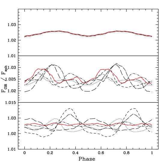
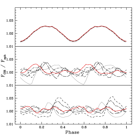
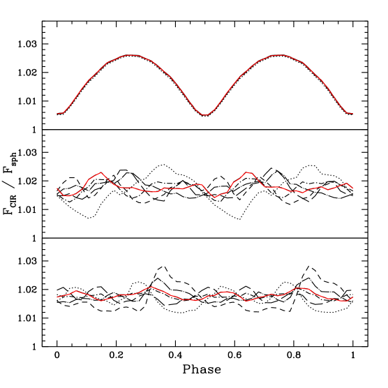
Figure 2: Model calculations for the radio flux as a function of rotational phase from a wind threaded by an equatorial CIR. From left to right, the panels are for 3 different viewing inclinations of $i=30^{\circ}$, $60^{\circ}$, and $90^{\circ}$. From top to bottom, the 3 panels are for different stellar rotation rates. The light curves are for different wavelengths, with red being the longest wavelength of the simulation at 31.6 cm and black dotted being the shortest at 1 mm (see text for more details). The curves are fluxes normalized to that of a spherical wind at each respective wavelength and plotted with rotation phase. Tab. LABEL:tab1 details specific parameters for each panel.

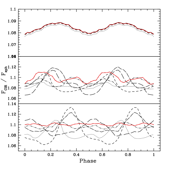
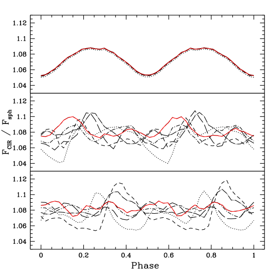
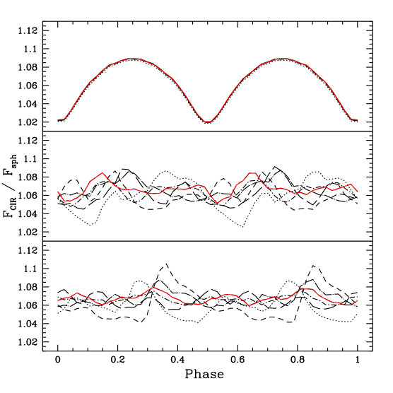
Figure 3: Same as Fig. 2, but with a different density contrast (see Tab. LABEL:tab1).

3 Discussion

Using the model of the preceding section, we simulated a large number of radio light curves. The parameter space is extensive, including the half-opening angle $\beta_{0}$, the viewing inclination $i_{0}$, the wind optical depth $\tau_{0}$, the co-latitude of the CIR $\vartheta$, the stellar rotation speed $v_{\rm rot}$ relative to the wind speed, and the density contrast between the CIR and the wind $\eta$. Note that the latter is defined as

$$\eta=\frac{n_{CIR}-n_{\rm sph}}{n_{\rm sph}},$$ (18)

where $n_{CIR}$ is the number density inside the CIR structure, and $n_{\rm sph}$ is the number density in the otherwise spherical wind. It is assumed that $\eta$ is a constant across the CIR, and with distance from the star. In addition to all these parameters, one further expects the detailed characteristics of the radio light curve to be a function of wavelength. Finally, one could even allow for multiple CIRs in the wind.

To keep the parameter space manageable, we have adopted a few simplications. First, we consider a wind with just one equatorial CIR, hence $\vartheta=90^{\circ}$. Second, noting that a pole-on view produces no variation of flux with rotational phase, we evaluate simulations for just three viewing inclinations of $i_{0}=30^{\circ}$ (nearly pole-on), $60^{\circ}$ (mid-perspective), and $90^{\circ}$ (edge-on). We consider only two density contrasts of $\eta=3$ and 9. We also consider just two half-width opening angles of $\beta_{0}=15^{\circ}$ and $25^{\circ}$.

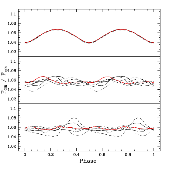
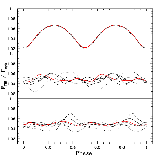
Figure 4: Same as Fig. 2, but now with a different opening angle (see Tab. LABEL:tab1).

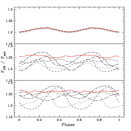
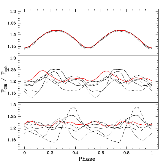
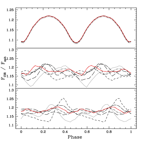
Figure 5: Same as Fig. 4, but now with a different density contrast (see Tab. LABEL:tab1).

Finally, we allow for three rotation speeds of 0, 52, and 175 km s^-1. A near-zero rotation speed represents a strict conical CIR. Consequently, the structure has no curvature, so the perturbation to the wind is self-similar with wavelength. The other two values represent low and medium rotations. A fast rotation case is not included for reasons that will soon be explained. In all models the wind terminal speed is fixed at $v_{\infty}=1750$ km s^-1, an intermediate value among WR stars, considering WN and WC subtypes.

Figures 2-5 display the model light curves and Table LABEL:tab1 details the various model parameters corresponding to the figures. In all cases, the spherical wind is assumed to have the same optical scale of $\tau_{0}=1.25\times 10^{5}$ at $\lambda=1$ cm. This value was chosen as typical of WR stars. The basis for this value derives from Figure 6 which displays a histogram for $r_{1}/R_{\ast}$ for both WN and WC stars using stellar and wind parameters from Hamann et al. (2019) and Sander et al. (2019) respectively. In calculating $r_{1}/R_{\ast}$ shown in this figure, representative values were adopted for mean molecular weights of WN and WC stars.

A typical volume filling factor of $f_{V}=0.1$ was adopted. Overall, an average value of $\langle r_{1}/R_{\ast}\rangle=35$ was determined. While there is some tail in the histogram, there is a fairly tight average value for the majority of stars. Our selection of a single $\tau_{0}$ corresponds to this typical value for $r_{1}/R_{\ast}$.

Turning back to the model light curves in Figures 2-5, each figure shows 3 sets of panels. The left set is for $i=30^{\circ}$; the center set is for $i=60^{\circ}$; and the right set is for $i=90^{\circ}$. For a given inclination, each of the 3 panels display radio light curves for different rotational phases. The top panel is for near-zero rotation speed; middle is for the low speed case; bottom is for the modest speed case. Table LABEL:tab1 identifies the moderl parameters for each panel, by identifying the figure, the set of panels (left, center, or right), and the specific panel (top, middle or “mid”, and bottom or “bot”). All light curves are plotted as fluxes normalized to what a strictly spherical wind would produce at the same wavelength. Each panel has multiple light curves for different wavelengths. The wavelengths range from 1 mm (dotted line) to 31.6 cm (red line) in logarithmic intervals of 0.5 dex.

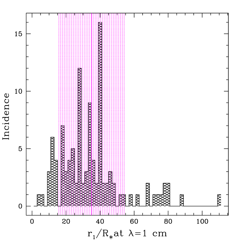
Figure 6: Shows the distribution of radio photospheres at $\lambda=1$ cm for single Galactic WN and WC stars. The vertical magenta line is the average for the distribution. The hashed magenta zone is $\pm 1$ standard deviation about the average for the distribution. Refer to text for further details.

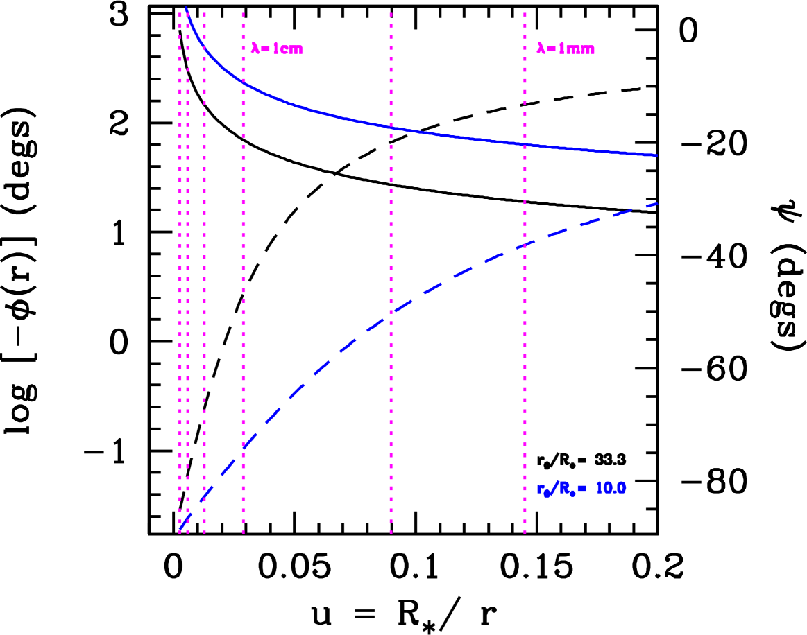
Figure 7: The left axis shows the wrapping of the CIR, $\phi$, in degrees in the log shown as the solid curve. The black and blue curves are for winding radii, $r_{0}/R_{\ast}$, as indicated; these correspond to the slower and faster rotation speeds associated with the light curves of Figs. 2-5. Note that 1 full wrapping of the CIR about the star is $360^{\circ}$ or about 2.56 in the log. The right axis is for the orientation of the unit tangent vector to the CIR, with $\psi=0^{\circ}$ being radial and $\psi=-90^{\circ}$ being backward azimuthal. The solutions for $\psi$ are displayed as dashed lines. The vertical magenta lines are for $r_{1}/R_{\ast}$ at the 6 wavelengths used for the light curve simulations, with the 1 mm and 1 cm lines labeled.

The results of the simulations can be summarized in four main points:

1. In all cases a CIR produces a flux offset. This is the same effect that stochastic clumping would have on the wind. In effect, a CIR can be considered as a clump with an organized geometry that produces systematic effects with rotation. The extent of the excess relative to a spherical wind scales with the gross properties of the CIR, such as density contrast $\eta$ and opening angle. For the parameters used in this study, excesses range from a few percent up to a few tens of percent. However, in the radio band, the presence of a CIR is betrayed through cyclic radio variability, with detectability set by the peak-to-trough variations of the excess. Those variations tend to be on the order of 10% or less, again for the adopted parameters.

2. The top panels of each figure is for a conical CIR. The assumption here is that rotation is so slow that the CIR has essentially no curvature. Two points are notable. First, we expect two peaks per rotation corresponding to when the CIR is in the plane of the sky. The simulations adopt zero phase as being when the footpoint of the CIR is on the near-side of the star. Then phase of 0.5 has the footpoint rear of the star; 0.25 has the footpoint in the plane of sky; and 0.75 is also in the sky plane but opposite of 0.25. The sense of rotation is counterclockwise as seen from above, hence if viewed edge-on, phase of 0.25 is rightside in the sky, and 0.75 is leftside, with the rotation axis lying in the plane of the sky and directed up to define right and left. Recall that the radio photosphere grows in extent with increasing wavelength. The absence of curvature for a conical CIR means that at every wavelength, the light curve samples the exact same relative geometry (i.e., the CIR is azimuthally aligned with its footpoint at all radii).

3. The middle and bottom panels allow for curvature of the CIR. With increasing radius, the CIR is becoming more “wound up”. At short wavelengths the radio photosphere forms where the CIR is less wound up; at long wavelengths, the photosphere is sampling a CIR that has a greater degree of spiral morphology, which depends on the ratio $v_{\rm rot}/v_{\infty}$. In general, this means that the emergence of the CIR at the wavelength-dependent photosphere becomes increasing lagged in azimuth as compared to the CIR footpoint. For example, when the footpoint is at a phase of 0.25, the CIR is backwinding and could emerge at the radio photosphere more in front of the star.

4. The asymptotic effect of a highly wound CIR is no longer to produce a variation with rotational phase. There is still an excess of flux above the spherical value, yet the light curve develops a variety of small peaks and troughs. Variability is suppressed because many wrappings of the CIR means that the projected radio photosphere, if it could be resolved, looks mostly the same at every wavelength. The many wrappings approximate a structure that becomes nearly axisymmetric. This can be seen in long-wavelength light curves (red) for the bottom panels. And it is why fast rotation speed cases were not included in the study, since these would only give low-variability behavior.

To illustrate how different wavelengths probe different geometries of the wind, Figure 7 displays the radii of the radio photospheres for the six wavelengths used with the simulated light curves in relation to how wrapped up the CIR has become. The horizontal axis is inverse radius, $u$, in the wind. The vertical magenta lines are the $u_{1}=R_{\ast}/r_{1}(\lambda)$ values for the six wavelengths, with 1 mm and 1 cm cases labeled. The leftside axis is for the azimuth of the center of the CIR as a function of radius from equation (12). However, it is plotted here in the log of $-\phi$, since by convention the CIR is backwinding relative to the stellar rotation. (Note that $-\phi=360^{\circ}$ is 2.56 in the log.) The rightside axis is for the orientation, $\psi$ of the local tangent to the CIR, with

$$\tan\psi=\frac{v_{\phi}(r)-\Omega\,r}{v_{\rm r}}.$$ (19)

If the CIR were radial, $\psi=0^{\circ}$; if it were purely azimuthal, $\psi=-90^{\circ}$, with the negative appearing because the CIR is backwinding.

Figure 7 shows two sets of curves. Black and blue colors are for values of the winding radius, $r_{0}$, as indicated in the figure. Solid is for $\phi$ and dashed is for $\psi$. The figure makes clear that owing to the increasing opacity with wavelength, radio data probe different degrees of curvature of the CIR, possibly even multiple wrappings, with $\lambda$.

4 Conclusion

There is unambiguous evidence today that radiatively driven winds are far more complex than the homogeneous, spherically symmetric flows originally envisioned (e.g. Castor et al., 1975). Instead, they have been shown to contain optically thick structures which may be quite small (micro-structures) or very large (macro-structures). Unraveling the details of these flows is a prerequisite to translating observational diagnostics into reliable physical quantities such as mass-loss rates. To progress, a firm grasp of the underlying physical mechanisms that determine the wind structures is needed. Specifically, the passage of CIR spiral arms across the line of sight to the stellar disk accounts for the wind line UV variability, and in that context they undoubtedly strongly affect the observational diagnostics used to determine the true mass-loss rates. The CIR density enhancements also provide a potentially powerful, but untested, means for producing radio variability.

We have demonstrated here that temporal radio continuum (multi-frequency) datasets can potentially provide a powerful new key to developing a coherent picture of wind flows, their large-scale structure and how they fit together. It is important to note that several simplifications have been invoked in order to facillitate a broad parameter study in terms of CIR geometry, density compression, and viewing inclination along with creating simulated multi-wavelength light curves. We recognize that hydrodynamic models for CIRs show not only compressions but also rarefactions. We anticipate a follow-up study to explore the impact of rarefactions for the light curves. A sector of depressed density acts in opposition to a sector where density is enhanced. The latter extends the radio photosphere; the former contracts it. One may expect that a rarefaction will lower the overall radio excess of a wind with a CIR as compared to a spherical wind. Correspondingly, variability is driven by how the projected radio photosphere changes with rotational phase. With both extension and contraction available, inclusion of rarefaction may increase the relative variability, although this is likely sensitive to viewing inclination.

What has been demonstrated is that new perspectives on large-scale wind structure can be provided by monitoring the radio continuum emission of WR and luminous O stars simultaneously at multi-radio bands (e.g., 1 cm, 6 cm, and 21 cm) over CIR (essentially stellar rotation) timescales. The variability from a CIR derives from a phase dependence of the projected and non-centrosymmetric photosphere with rotation. For an equatorial CIR that is quite over-dense compared to its surroundings, the overall variation in flux for the unresolved source could achieve variations of 10–20%. From an observational perspective, curvature due to a spiral-CIR results in the development of a potentially exploitable phase lag, provided the bands have sufficient dynamic range in wavelength and are monitored contemporaneously. Another prediction of the model is that the amplitude decreases as the photosphere grows with wavelength, because more winding up of the spiral leads to less relative variability. So at short wavelength, there are two peaks because the CIR is more nearly like a cone and results in maximum flux excess when the cone is on either side of the star in the plane of sky. By contrast, at truly long wavelengths, which diagnose a CIR that is very wrapped up, there is indeed a flux enhancement but no variability.

Ultimately, powerful radio astronomy facilities such as the Square Kilometre Array (SKA) will open up new avenues such time-domain surveys of massive star winds. The interpretation of these very rich datasets will require an understanding of the contribution of large-scale wind structures to the thermal and non-thermal emission in the radio.

Data Availability Statement

The data underlying this article will be shared on reasonable request to the corresponding author.

References

- Aldoretta et al. (2016) Aldoretta E. J., et al., 2016, MNRAS, 460, 3407
- Blomme (2011) Blomme R., 2011, Bulletin de la Societe Royale des Sciences de Liege, 80, 67
- Carlberg (1980) Carlberg R. G., 1980, ApJ, 241, 1131