The dynamics of liquid films, as described by the diffuse-interface model

Abstract

The dynamics of a thin layer of liquid, between a flat solid substrate and an infinitely-thick layer of saturated vapor, is examined. The liquid and vapor are two phases of the same fluid, governed by the diffuse-interface model. The substrate is maintained at a fixed temperature, but in the bulk of the fluid the temperature is allowed to vary. The slope $\varepsilon$ of the liquid/vapor interface is assumed to be small, as is the ratio of its thickness to that of the film. Three asymptotic regimes are identified, depending on the vapor-to-liquid density ratio $\rho_{v}/\rho_{l}$. If $\rho_{v}/\rho_{l}\sim 1$ (which implies that the temperature is comparable, but not necessarily close, to the critical value), the evolution of the interface is driven by the vertical flow due to liquid/vapor phase transition, with the horizontal flow being negligible. In the limit $\rho_{v}/\rho_{l}\rightarrow 0$, it is the other way around, and there exists an intermediate regime, $\rho_{v}/\rho_{l}\sim\varepsilon^{4/3}$, where the two effects are of the same order. Only the $\rho_{v}/\rho_{l}\rightarrow 0$ limit is mathematically similar to the case of incompressible (Navier–Stokes) liquids, whereas the asymptotic equations governing the other two regimes are of different types.

I Introduction

The diffuse-interface model (DIM) originates from the idea of van der Waals van der Waals (1893) and Korteweg Korteweg (1901) that intermolecular attraction in fluids can be modeled by relating it to macroscopic variations of the fluid density. In recent times, this approach was incorporated into hydrodynamics: more comprehensive models have been developed for multi-component fluids with variable temperature Anderson, McFadden, and Wheeler (1998); Thiele, Madruga, and Frastia (2007) – and simpler ones, for single-component isothermal fluidsPismen and Pomeau (2000)) or single-component isothermal and incompressible fluids Jasnow and Viñals (1996); Jacqmin (1999); Ding and Spelt (2007); Madruga and Thiele (2009) (in the last case, the van der Waals force does not depend on the (constant) density, but on a certain “order parameter” satisfying the Cahn–Hilliard equation).

Various versions of the DIM have been used in applications, such as nucleation, growth, and collapse of vapor bubbles Magaletti, Marino, and Casciola (2015); Magaletti et al. (2016); Gallo, Magaletti, and Casciola (2018); Gallo et al. (2020), drops impacting on a solid wall Gelissen et al. (2020), and contact lines in fluids Seppecher (1996); Ding and Spelt (2007); Yue, Zhou, and Feng (2010); Yue and Feng (2011); Sibley et al. (2013a, b, 2014); Kusumaatmaja, Hemingway, and Fielding (2016); Fakhari and Bolster (2017); Borcia et al. (2019).

When studying contact lines, a boundary condition describing the interaction of the fluid and substrate is needed. Two version of such have been suggested: one involving the near-substrate density Seppecher (1996) and its normal derivative, and another prescribing just the density Pismen and Pomeau (2000). The former is based on minimisation of the wall free energy Pismen and Pomeau (2000), whereas the latter can be obtained through an asymptotic expansion of the non-local representation of the van der Waals force Benilov (2020a). In the present paper, the latter (simpler) boundary condition is used.

The DIM has been also adapted for the case of liquid films, where the liquid phase is confined to a thin layer bounded by a liquid/vapor interface and a solid substrate. Assuming that the flow is isothermal and the saturated-vapor density $\rho_{v}$ is much smaller that the liquid density $\rho_{l}$, Pismen and Pomeau Pismen and Pomeau (2000) derived an asymptotic version of the DIM similar to the thin-film approximation of the Navier–Stokes equations for incompressible fluids.

It has been argued, however, that in some, if not most, common fluids including water, liquid/vapor interfaces are not isothermal. Using a non-isothermal version of the DIM, Refs. Benilov (2020a, b) estimated the density and pressure change near the interface and showed that the resulting temperature change is order-one. It is unclear, however, whether this conclusion affects liquid films, as a thin liquid layer can behave differently from the general case – especially, if the substrate is maintained at a fixed temperature, acting as a thermostat for the adjacent fluid.

There are two more omissions in the existing literature on liquid films with a diffuse interface. Firstly, no thin-film models exist for the regime with $\rho_{v}\sim\rho_{l}$ observed at medium and high temperatures. Secondly, no-one has examined the implications for films of a recently-identified contradiction between the DIM and the Navier–Stokes equations: as shown in Ref. Benilov (2020c), the former does not admit solutions describing static two-dimensional sessile drops (also called liquid ridges), whereas the latter do. A similar comparison between the thin-film asymptotics of the two models should clarify the nature of the discrepancy, as asymptotic models are much simpler than the exact ones.

The present paper tackles the above omissions. It is shown that, if $\rho_{v}\sim\rho_{l}$, the heat released (consumed) due to the fluid compression (expansion) near the interface makes non-isothermality important, so the thin-film asymptotics in this case differs from that derived in Ref. Pismen and Pomeau (2000). In the limit $\rho_{v}/\rho_{l}\rightarrow 0$, however, liquid films are essentially isothermal and the thin-film approximation of the DIM coincides with that of the Navier–Stokes equations. This implies that liquid ridges exist in the former model as quasi-static states, i.e., they evolve, but so slowly that the evolution is indistinguishable from, say, evaporation.

The present paper is structured as follows. In Sect. II, the problem is formulated mathematically, and in Sect. III, the simplest case of static interfaces is examined. The regimes $\rho_{v}\sim\rho_{l}$ and $\rho_{v}\ll\rho_{l}$ are examined in Sects. IV and V, respectively. Since these sections include a lot of cumbersome algebra, a brief summary of the results, plus their extensions to three-dimensional flows, are presented in Sect. VI.

II Formulation

Consider a compressible fluid flow characterized by the density $\rho(\mathbf{r},t)$, velocity $\mathbf{v}(\mathbf{r},t)$, and temperature $T(\mathbf{r},t)$, where $\mathbf{r}$ is the position vector and $t$, the time. Let the pressure $p$ be related to $\rho$ and $T$ by the the van der Waals equation of state,

$$p=\frac{RT\rho}{1-b\rho}-a\rho^{2},$$ (1)

where $R$ is the specific gas constant, and $a$ and $b$ are fluid-specific constants ($b$ is the reciprocal of the maximum allowable density). Eq. (1) was chosen for its simplicity, with all of the results obtained below being readily extendable to general non-ideal fluids.

The diffuse-interface model in application to compressible Newtonian fluid is Anderson, McFadden, and Wheeler (1998)

$$\frac{\partial\rho}{\partial t}+\boldsymbol{\boldsymbol{\nabla}}\cdot\left(\rho\mathbf{v}\right)=0,$$ (2)

$$\rho\left[\frac{\partial\mathbf{v}}{\partial t}+\left(\mathbf{v}\cdot\boldsymbol{\boldsymbol{\nabla}}\right)\mathbf{v}\right]+\boldsymbol{\boldsymbol{\nabla}}p-\boldsymbol{\boldsymbol{\nabla}}\cdot\boldsymbol{\Pi}=K\rho\boldsymbol{\boldsymbol{\nabla}}\nabla^{2}\rho,$$ (3)

$$\rho c_{V}\left(\frac{\partial T}{\partial t}+\mathbf{v}\cdot\boldsymbol{\boldsymbol{\nabla}}T\right)+\left[\mathbf{I}\left(p+a\rho^{2}\right)-\boldsymbol{\Pi}\right]:\boldsymbol{\boldsymbol{\nabla}}\mathbf{v}\\ -\boldsymbol{\boldsymbol{\nabla}}\cdot\left(\kappa\boldsymbol{\boldsymbol{\nabla}}T\right)=0,$$ (4)

where $\mathbf{I}$ is the identity matrix,

$$\boldsymbol{\Pi}=\mu_{s}\left[\boldsymbol{\boldsymbol{\nabla}}\mathbf{v}+\left(\boldsymbol{\boldsymbol{\nabla}}\mathbf{v}\right)^{T}-\frac{2}{3}\mathbf{I}\left(\boldsymbol{\boldsymbol{\nabla}}\cdot\mathbf{v}\right)\right]+\mu_{b}\,\mathbf{I}\left(\boldsymbol{\boldsymbol{\nabla}}\cdot\mathbf{v}\right)$$ (5)

is the viscous stress tensor, $K$ is the so-called Korteweg parameter, $\mu_{s}$ ($\mu_{b}$) is the shear (bulk) viscosity, $c_{V}$ is the specific heat capacity, and $\kappa$, the thermal conductivity. Note that, generally, $\mu_{s}$, $\mu_{b}$, $c_{V}$, and $\kappa$ depend on $\rho$ and $T$, whereas $K$ is a constant.

In what follows, two-dimensional flows will be mainly explored, so $\mathbf{r}=\left[x,z\right]$ and $\mathbf{v}=\left[u,w\right]$ where $x$ and $u$ are the horizontal components of the corresponding vectors, and $z$ and $w$ are their vertical components. The three-dimensional extensions of the results obtained will be presented without derivation in Sect. VI.

Assume that the fluid is bounded below by a solid substrate located at $z=0$, so the flow is constrained by

$$\mathbf{v}=\mathbf{0}\qquad\text{at}\qquad z=0,$$ (6)

$$T=T_{0}\qquad\text{at}\qquad z=0,$$ (7)

$$\rho=\rho_{0}\qquad\text{at}\qquad z=0.$$ (8)

(6) is the no-flow boundary condition, (7) implies that the substrate is maintained at a fixed temperature $T_{0}$, and the near-wall density $\rho_{0}$ in (8) is a phenomenological parameter (in the diffuse-interface model Pismen and Pomeau (2000); Benilov (2020a), it is assumed to be known). Note that the parameter $\rho_{0}$ is specific to the fluid–substrate combination under consideration and is uniquely related to the contact angle.

Given a suitable initial condition, the boundary-value problem (1)-(8) determines the unknowns $\rho(\mathbf{r},t)$, $\mathbf{v}(\mathbf{r},t)$, and $T(\mathbf{r},t)$.

III Static films

Before examining the evolution of liquid films, it is instructive to briefly review the properties of static films.

Letting $\mathbf{v}=\mathbf{0}$ and $\partial\rho/\partial t=0$, and taking into account that only isothermal films can be static (hence, $T=T_{0}$), one can reduce Eqs. (1)-(5) to a single equation

$$RT_{0}\left(\ln\frac{b\rho}{1-b\rho}+\frac{1}{1-b\rho}\right)-2a\rho-K\nabla^{2}\rho=G,$$ (9)

where $G$ is a constant of integration (physically, the free-energy density). Once Eq. (9) is complemented with boundary conditions, one can determine $G$ together with the solution $\rho$.

The one- and two-dimensional solutions of Eq. (9) will be examined in Sects. III.1 and III.2, respectively.

III.1 Films with flat interfaces

Let $\rho$ be independent of $x$, so that $\rho(z)$ describes a flat interface parallel to the substrate. The following nondimensional variables will be used:

$$\rho_{nd}=b\rho,\qquad z_{nd}=\frac{z}{z_{0}},$$ (10)

where

$$z_{0}=\sqrt{\frac{K}{a}}$$ (11)

is, physically, the characteristic thickness of liquid/vapor interfaces. Estimates of $z_{0}$ for specific applications presented in Refs. Magaletti et al. (2016); Benilov (2020a) show that $z_{0}$ is on a nanometer scale; hereinafter it will be referred to as “microscopic”.

It is convenient to also introduce the nondimensional analogues of the parameters $\rho_{0}$ and $G$,

$$\left(\rho_{0}\right)_{nd}=b\rho_{0},\qquad G_{nd}=\frac{b}{a}G.$$ (12)

In nondimensional form, Eq. (9) is (the subscript _nd omitted)

$$\tau\left(\ln\frac{\rho}{1-\rho}+\frac{1}{1-\rho}\right)-2\rho-\frac{\mathrm{d}^{2}\rho}{\mathrm{d}z^{2}}=G,$$ (13)

where the first two terms on the left-hand side represent the nondimensional free-energy density of the van der Waals fluid, and

$$\tau=\frac{RT_{0}b}{a}$$ (14)

is the nondimensional temperature. The nondimensional version of the boundary condition (8) will not be presented as it looks exactly as its dimensional counterpart. One should also impose the requirement of zero Korteweg stress at infinity,

$$\frac{\mathrm{d}\rho}{\mathrm{d}z}\rightarrow 0\qquad\text{as}\qquad z\rightarrow\infty.$$ (15)

Due to the presence of the undetermined constant $G$, Eq. (13) and the boundary conditions (8), (15) do not fully determine the solution. The most convenient way to fix $\rho(z)$ consists in prescribing the height $h$ of the interface through the requirement

$$\rho(h)=\frac{\max\left\{\rho(z)\right\}+\min\left\{\rho(z)\right\}}{2}.$$ (16)

In what follows, the solution of the boundary-value problem (13), (8), (15)-(16) will be denoted by $\rho(z|h)$. Several examples of $\rho(z|h)$ with increasing $h$ are shown in Fig. 1.

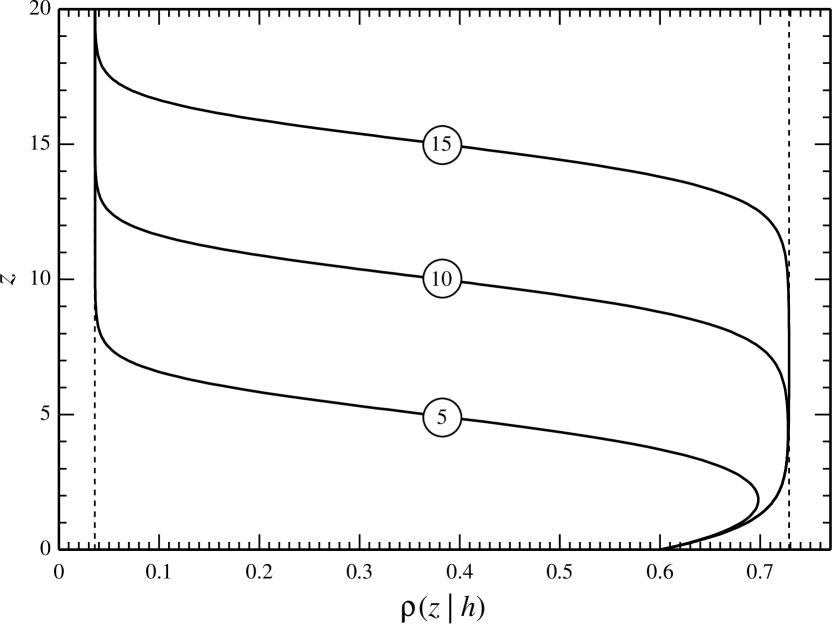
Figure 1: The function $\rho(z|h)$ [determined by (13), (8), (15)-(16)] for $\tau=0.2$ and $\rho_{0}=0.6$. The curves are labelled with the corresponding values of $h$. The dotted lines show $\rho_{v}$ and $\rho_{l}$.

In this work, the following properties of $\rho(z|h)$ will be needed:

(1) Since $z$ was nondimensionalized on a microscopic scale, macroscopic films correspond to $h\gg 1$, making this limit important for applications – both industrial (e.g., paint or polymer coating) and natural (e.g., rainwater flowing down a rockface).

For large $h$, the interface is located far from the substrate, so the interfacial profile is similar to that in an unbounded fluid. Mathematically, this means

$$\rho(z|h)\rightarrow\bar{\rho}(z-h)\qquad\text{as}\qquad z,h\rightarrow\infty,$$ (17)

where $\bar{\rho}(z)$ satisfies the same equation as $\rho(z,h)$ and the open-space boundary conditions,

$$\tau\left(\ln\frac{\bar{\rho}}{1-\bar{\rho}}+\frac{1}{1-\bar{\rho}}\right)-2\bar{\rho}-\frac{\mathrm{d}^{2}\bar{\rho}}{\mathrm{d}z^{2}}=G,$$ (18)

$$\bar{\rho}(z) \rightarrow\rho_{l}\qquad\,\text{as}\qquad z\rightarrow-\infty,$$ (19)

$$\bar{\rho}(z) \rightarrow\rho_{v}\qquad\text{as}\qquad z\rightarrow\infty,$$ (20)

$$\bar{\rho}(0)=\frac{\rho_{l}+\rho_{v}}{2}.$$ (21)

Eqs. (18)-(21) fix $\bar{\rho}(z)$, as well as $\rho_{v}$ and $\rho_{l}$ (which represent the nondimensional densities of saturated vapor and liquid, respectively).

As observed in Ref. Pismen and Pomeau (2000), the influence of the substrate decays exponentially with the distance, which implies that the asymptotic formula (17) is accurate even for moderate (logarithmically large) $h$. However, even though $\bar{\rho}(z-h)$ approximates $\rho(z|h)$ well in the interfacial region, $\bar{\rho}(z-h)$ does not generally satisfy the boundary condition at the substrate. The only exception is the case where $\rho_{0}$ is close to $\rho_{l}$, which implies that near the substrate, $\rho(z|h)\approx\bar{\rho}(z-h)+\mathcal{O}(\varepsilon)$, where $\varepsilon=\rho_{l}-\rho_{0}$. Merging this result with (17) (which is exponentially accurate in both $1/h$ and $\varepsilon$), one obtains

$$\rho(z|h)=\bar{\rho}(z-h)+\mathcal{O}(\varepsilon)\qquad\text{if}\qquad h\gg 1,$$ (22)

which applies to all $z$. Note also that the limit of small $\varepsilon$ is important as it corresponds to the approximation of small contact angle (more details are given below).

(2) $\rho_{l}$ and $\rho_{v}$ can be computed without calculating $\bar{\rho}(z)$, through the so-called Maxwell construction. In the low-temperature limit $\tau\rightarrow 0$, it yields (see Appendix A)

$$\rho_{l}=\frac{1+\sqrt{1-4\tau}}{2}+\mathcal{O}(\operatorname{e}^{-1/\tau}),$$ (23)

$$\rho_{v}=\frac{1+\sqrt{1-4\tau}}{1-\sqrt{1-4\tau}}\operatorname{e}^{-1/\tau}+\mathcal{O}(\tau^{-1}\operatorname{e}^{-2/\tau}).$$ (24)

Thus, if $\tau$ is small, $\rho_{v}$ is exponentially small.

If $\tau$ increases, $\rho_{v}$ grows and $\rho_{l}$ decays; eventually, they merge at the critical point $\left(\rho_{v}\right)_{cr}=\left(\rho_{l}\right)_{cr}=1/3$, $\tau_{cr}=8/27$. For larger $\tau$, only one phase exists, so liquid films do not exists.

For $\tau\ll 1$, one can also obtain an exponentially accurate expression for the whole solution $\bar{\rho}(z)$, but it is bulky and implicit. In what follows, an algebraically accurate but explicit expression will be used,

$$\bar{\rho}(z)=\left\{\begin{tabular}[c]{ll}$1+\mathcal{O}(\tau\ln\tau)\vskip 6.0pt plus 2.0pt minus 2.0pt$&if$\qquad z\leq-2^{-3/2}\pi,$\\ $\frac{1}{2}\left(1-\sin 2^{1/2}z\right)+\mathcal{O}(\tau\ln\tau)\vskip 6.0pt plus 2.0pt minus 2.0pt\qquad$&if$\qquad z\in\left[-2^{-3/2}\pi,~{}2^{-3/2}\pi\right],$\\ $0+\mathcal{O}(\tau\ln\tau)$&if$\qquad z\geq 2^{-3/2}\pi.$\end{tabular}\ \right.$$ (25)

This solution follows from Eq. (18) with $\tau=0$ and the boundary conditions (19)-(20) with $\rho_{l}=1$ and $\rho_{v}=0$.

The low-temperature limit is important, as $\tau$ is indeed small for many common liquids. For water at $20^{\circ}\mathrm{C}$, for example, estimates of $\tau$ vary from $0.064$ to $0.14$ (depending on the equation of state used – see Refs. Benilov (2020a, b)).

(3) In what follows, the function

$$\rho^{\prime}(h)=\frac{1}{\rho_{l}-\rho_{0}}\left[\frac{\mathrm{d}\rho(z|h)}{\mathrm{d}z}\right]_{z=0}$$ (26)

plays an important role. It can be readily computed – see examples shown in Fig. 2. Evidently, $\rho^{\prime}(h)$ is bounded above, and its precise upper bound is (see Appendix B)

$$\rho^{\prime}(h)<\frac{\sqrt{2}}{\rho_{l}-\rho_{0}}\\ \times\sqrt{\tau\left[\rho_{0}\ln\dfrac{\rho_{0}\left(1-\rho_{v}\right)}{\rho_{v}\left(1-\rho_{0}\right)}-\frac{\rho_{0}-\rho_{v}}{1-\rho_{v}}\right]-\left(\rho_{0}-\rho_{v}\right)^{2}}.$$ (27)

As follows from Fig. 2, $\rho^{\prime}(h)$ tends to its maximum as $h\rightarrow\infty$. What happens in this limit with $\rho(z|h)$ has been illustrated in Fig. 1.

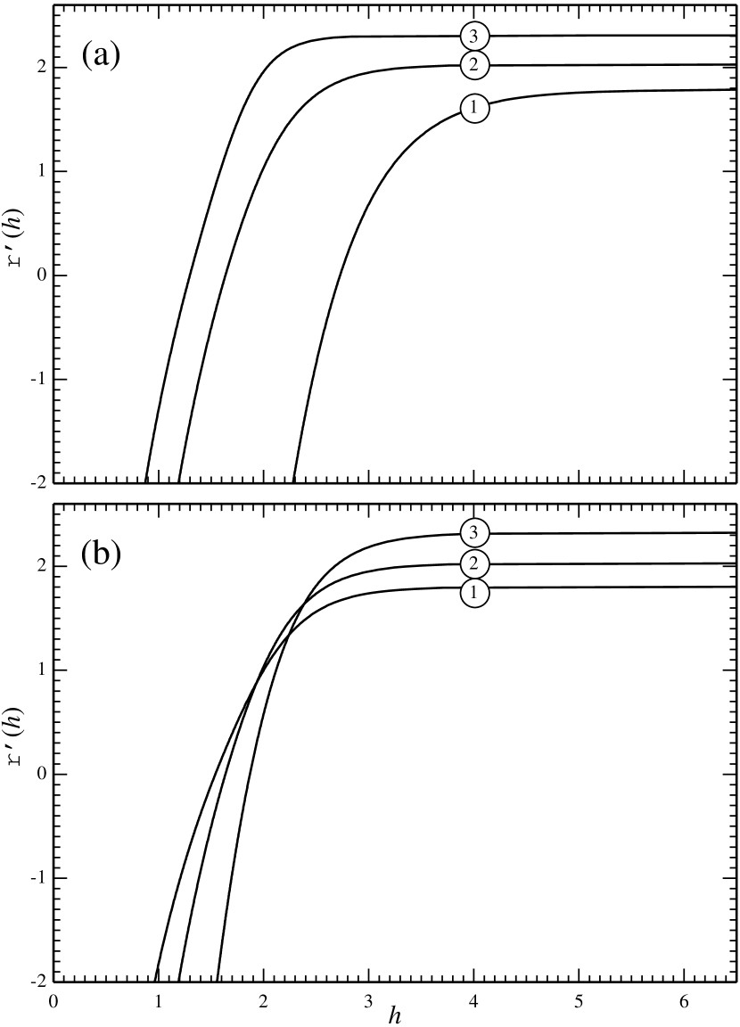
Figure 2: The function $\rho^{\prime}(h)$. Panel (a): $\rho_{0}=0.8$, curves 1-3 correspond to $\tau=0.15,~{}0.1,~{}0.05$; Panel (b): $\tau=0.1$, curves 1-3 correspond to $\rho_{0}=0.75,~{}0.8,~{}0.85$.

Note that $\rho^{\prime}(h)$ remains order-one in the limit $\rho_{0}\rightarrow\rho_{l}$. Indeed, letting

$$\rho_{0}=\rho_{l}-\varepsilon$$ (28)

and expanding estimate (27) in powers of $\varepsilon$, one can take into account the Maxwell construction (104)-(105) and see that the first two orders of the expansion in $\varepsilon$ vanish, so that (27) becomes

$$\rho^{\prime}(h)<\sqrt{\frac{\tau}{\rho_{l}\left(1-\rho_{l}\right)^{2}}-2}+\mathcal{O}(\varepsilon).$$ (29)

The limit $\varepsilon\ll 1$ is particularly important, as it corresponds to the contact angle being small Pismen and Pomeau (2000).

III.2 Films with slightly curved interfaces

Consider the full (two-dimensional) equation (9) and assume that the interface is curved, but its slope is small. This can only occur if the contact angle is small – which, in turn, implies that $\rho_{0}$ is close to, but still smaller than, the liquid density $\rho_{l}$.

Given scaling (10) of the vertical coordinate $z$, the scaling of the horizontal coordinate should be

$$x_{nd}=\frac{\varepsilon x}{z_{0}},$$ (30)

where $\varepsilon\ll 1$ is related to the physical parameters by (28), but also playes the role of the slope of the interace. Rewriting Eq. (9) in terms of the nondimensional variables (10)-(12) and (30), one obtains (the subscript _nd omitted)

$$\tau\left(\ln\frac{\rho}{1-\rho}+\frac{1}{1-\rho}\right)-2\rho-\varepsilon^{2}\frac{\partial^{2}\rho}{\partial x^{2}}-\frac{\partial^{2}\rho}{\partial z^{2}}=G.$$ (31)

In addition to the boundary condition (8) at the wall, a condition is required as $z\rightarrow\infty$. Assuming that the liquid film is bounded above by an infinite layer of saturated vapor, require

$$\rho\rightarrow\rho_{v}\qquad\text{as}\qquad z\rightarrow\infty.$$ (32)

This boundary condition is consistent with Eq. (31) only if

$$G=\tau\left(\ln\frac{\rho_{v}}{1-\rho_{v}}+\frac{1}{1-\rho_{v}}\right)-2\rho_{v}.$$ (33)

The difference between Eq. (31) and its one-dimensional counterpart (13) is $\mathcal{O}(\varepsilon^{2})$ – hence, the solution of the former can be sought using that of the latter,

$$\rho(x,z)=\rho(z|h)+\mathcal{O}(\varepsilon^{2}),$$ (34)

where $h=h(x)$ is an undetermined function. Physically, solution (34) describes a liquid film with a slowly changing thickness.

Let $h\gg 1$, in which case expressions (34) and (22) yield

$$\rho=\bar{\rho}(z-h)+\mathcal{O}(\varepsilon).$$ (35)

This approximation will be used everywhere in this paper. It applies to films whose dimensional thickness exceeds the thickness $z_{0}$ of the liquid/vapor interface given by (11) – hence, since $z_{0}$ is of on a nanometer scale, this assumption is not very restrictive.

There are two ways to determine $h(x)$. Firstly, one can expand the solution in $\varepsilon$, with the leading order determined by (35) – then try to find the next-to-leading-order solution. The latter is likely to exist only subject to $h(x)$ satisfying a certain differential equation.

Secondly, one can try to rearrange the exact boundary-value problem in such a way that all leading-order terms cancel; then substitute the leading-order solution (35) in the resulting equation(s). For the static case, the second approach is only marginally simpler – but, for evolving films, it is much simpler, and so will be used in both cases.

To eliminate the leading-order terms from Eq. (31), multiply it by $\partial\rho/\partial z$, integrate from $z=0$ to $z=\infty$, then take into account the boundary conditions (32), (8) and expression (33) for $G$. After straightforward algebra, one obtains

$$-\varepsilon^{2}\frac{\mathrm{d}}{\mathrm{d}x}\int_{0}^{\infty}\frac{\partial\rho}{\partial x}\frac{\partial\rho}{\partial z}\mathrm{d}z=C-\frac{1}{2}\left[\left(\frac{\partial\rho}{\partial z}\right)_{z=0}\right]^{2},$$ (36)

where

$$C=\tau\left[\rho_{0}\left(\ln\frac{\rho_{0}}{1-\rho_{0}}-\ln\frac{\rho_{v}}{1-\rho_{v}}\right)-\frac{\rho_{0}-\rho_{v}}{1-\rho_{v}}\right]\\ -\left(\rho_{0}-\rho_{v}\right)^{2}.$$ (37)

Next, substitute (28) into (37), expand it in $\varepsilon$, take into account the Maxwell construction (104)-(105), and thus obtain

$$C=\varepsilon^{2}\left[\frac{\tau}{2\rho_{l}\left(1-\rho_{l}\right)^{2}}-1\right]+\mathcal{O}(\varepsilon^{3}).$$ (38)

Observe that, even though the exact expression for $C$ involves $\rho_{v}$, the approximate one involves $\rho_{l}$ (which occurs due to the use of the Maxwell construction inter-relating these parameters).

Now, substitute the leading-order solution (35) into Eq. (36) and take into account (38). Omitting small terms, one obtains

$$\frac{\mathrm{d}}{\mathrm{d}x}\left(\sigma\frac{\mathrm{d}h}{\mathrm{d}x}\right)=\frac{\tau}{2\rho_{l}\left(1-\rho_{l}\right)^{2}}-1-\frac{1}{2}\rho^{\prime 2}(h),$$ (39)

where the function $\rho^{\prime}(h)$ is defined by (26) and (28), and

$$\sigma=\int_{0}^{\infty}\left[\frac{\partial\bar{\rho}(z-h)}{\partial z}\right]^{2}\mathrm{d}z.$$

Since $h\gg 1$, one can extend the above integral to $-\infty$ (without altering significantly its value),

$$\sigma=\int_{-\infty}^{\infty}\left[\frac{\partial\bar{\rho}(z)}{\partial z}\right]^{2}\mathrm{d}z.$$ (40)

This expression does not depend on $h$ and coincides with the capillary coefficient (see Ref. Pismen and Pomeau (2000)).

Finally, substituting (38) into (39) one obtains

$$2\sigma\frac{\mathrm{d}^{2}h}{\mathrm{d}x^{2}}=\frac{\tau}{\rho_{l}\left(1-\rho_{l}\right)^{2}}-2-\rho^{\prime 2}(h).$$ (41)

This equation determines the profile $h(x)$ of a liquid film. Bar notation, it coincides with Eq. (42) of Ref. Pismen and Pomeau (2000), and they both are thin-film reductions of the requirement that a steady distribution of density must have homogeneous chemical potential.

III.3 Does Eq. (41) admit ridge solutions?

The most surprising feature of Eq. (41) is that it does not admit solutions describing two-dimensional sessile drops (also called liquid ridges). This conclusion is highly counter-intuitive, as the Navier–Stokes equations do admit such solutions. This paradox will be resolved in Sect. V.

To prove the nonexistence of ridge solutions, note that the DIM does not allow the substrate to be completely dry Pismen and Pomeau (2000). Hence, ridge solutions should involve a “precursor film”, i.e.,

$$h\rightarrow h_{pf}\qquad\text{as}\qquad x\rightarrow\pm\infty,$$ (42)

where $h_{pf}$ is the precursor film’s thickness. This boundary condition is consistent with Eq. (41) only if $h_{pf}$ satisfies either

$$\rho^{\prime}(h_{pf})=-\sqrt{\frac{\tau}{\rho_{l}\left(1-\rho_{l}\right)^{2}}-2}$$ (43)

or

$$\rho^{\prime}(h_{pf})=\sqrt{\frac{\tau}{\rho_{l}\left(1-\rho_{l}\right)^{2}}-2}.$$ (44)

It can be deduced from the Maxwell construction that

$$\frac{\tau}{\rho_{l}\left(1-\rho_{l}\right)^{2}}>2\qquad\text{if}\qquad\tau<\frac{8}{27},$$

hence, Eq. (43) admits a real solution for $h_{pf}$. Eq. (44), on the other hand, does not admit real solutions due to inequality (29).

The mere fact that there exists only one value of $h$ such that the right-hand side of Eq. (41) vanishes disallows the existence of ridge solutions. Indeed, let the ridge’s crest be located at $x=0$, i.e.,

$$\frac{\mathrm{d}h}{\mathrm{d}x}=0,\qquad h>h_{pf}\qquad\text{at}\qquad x=0,$$

and assume that $h(x)$ monotonically grows in $\left(-\infty,0\right)$ and decays in $\left(0,\infty\right)$. This implies existence of two inflection points, where $\mathrm{d}^{2}h/\mathrm{d}x^{2}=0$ and $h>h_{pf}$. The former condition can only hold if the right-hand side of Eq. (41) vanishes at the inflection points – which is, however, impossible since it vanishes only if $h=h_{pf}$.

If the ridge profile involves oscillations and, thus, several pairs of inflection points, the same argument applies to the farthest one from the crest (because $h$ at this inflection point certainly differs from $h_{pf}$). Overall, the conclusion about the nonexistence of thin ridges agrees with a similar result proved in Ref. Benilov (2020c) for arbitrary ridges. The physical implications of the non-existence of steady ridge solutions will be discussed in the end of Sect. V.3.

Eq. (41) still admits solutions such that

$$h\sim\theta x\qquad\text{as}\qquad x\rightarrow+\infty,$$ (45)

where the constant $\theta$ can be identified with the contact angle (strictly speaking, the contact angle equals $\arctan\theta$, but under the thin-film approximation $\arctan\theta\approx\theta$). Examples of the solution of the boundary-value problem (41), (42), (45) has been computed numerically and are shown in Fig. 3. Evidently, with increasing temperature, the precursor film becomes thicker (see Fig. 3a), whereas the contact angle becomes smaller (see Fig. 3b). The latter conclusion agrees with the results of Ref. Benilov (2020a) obtained for a realistic equation of state for water.

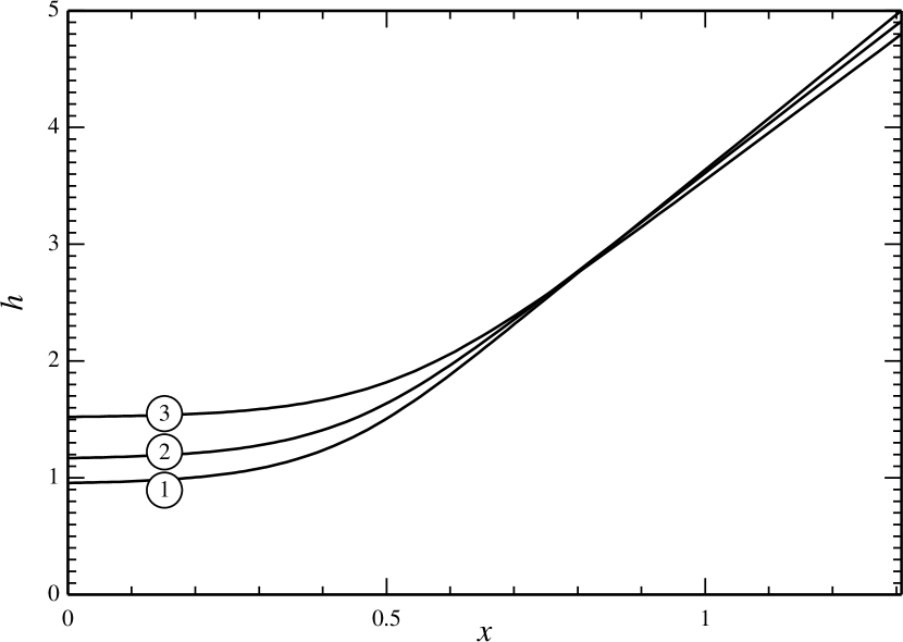
Figure 3: The solution of the boundary-value problem (41)-(42), (45) for $\rho_{0}=0.85$ and (1) $\tau=0.05$, (2) $\tau=0.1$, (3) $\tau=0.15$.

IV Evolving interfaces: the regime with $\rho_{v}\sim\rho_{l}$

Dynamics of liquid films depends strongly on the vapor-to-liquid density ratio. The regime $\rho_{v}/\rho_{l}=\mathcal{O}(1)$ – which occurs if $\tau=\mathcal{O}(1)$ (i.e., the dimensional temperature $T$ is comparable to the fluid’s critical temperature $T_{cr}$) – will be examined first. The reader will see that, in this case, diffuse-interface films behave very differently from their Navier–Stokes counterparts.

The asymptotic limit $T\ll T_{cr}$ will be examined in Sec. V.

IV.1 Nondimensionalization

In addition to the nondimensional versions of coordinates (10), density (12), and parameter $\rho_{0}$ (30), introduce

$$t_{nd}=\frac{\varepsilon^{2}v_{0}}{z_{0}}t,\qquad u_{nd}=\frac{u}{\varepsilon^{3}v_{0}},\qquad w_{nd}=\frac{w}{\varepsilon^{2}v_{0}},$$ (46)

$$T_{nd}=\frac{T}{T_{0}},\qquad p_{nd}=\frac{b^{2}}{a}p,$$ (47)

$$\left(\mu_{s}\right)_{nd}=\frac{\mu_{s}}{\mu_{0}},\qquad\left(\mu_{b}\right)_{nd}=\frac{\mu_{b}}{\mu_{0}},\qquad\kappa_{nd}=\frac{\kappa}{\kappa_{0}},$$ (48)

where the shear and bulk viscosities are assumed to be of the same order ($\mu_{s}\sim\mu_{b}\sim\mu_{0}$) and

$$v_{0}=\frac{az_{0}}{\mu_{0}b^{2}}$$ (49)

is the general-case velocity scale (which applies when the film’s slope $\varepsilon$ and thickness $h$ are both order-one). Note that the powers of $\varepsilon$ in (46) have been chosen through the trial-and-error approach, so that a consistent asymptotic model would be obtained in the end.

In terms of the nondimensional variables, the boundary-value problem (1)-(8) becomes (the subscript _nd omitted)

$$\frac{\partial\rho}{\partial t}+\framebox{$\varepsilon^{2}$}\frac{\partial\left(\rho u\right)}{\partial x}+\frac{\partial\left(\rho w\right)}{\partial z}=0,$$ (50)

$$\framebox{$\alpha\varepsilon^{4}$}\left(\frac{\partial u}{\partial t}+\framebox{$\varepsilon^{2}$}u\frac{\partial u}{\partial x}+w\frac{\partial u}{\partial z}\right)+\frac{1}{\rho}\frac{\partial}{\partial x}\left(\frac{\framebox{$\tau$}T\rho}{1-\rho}-\rho^{2}\right)-\frac{\partial}{\partial x}\left(\framebox{$\varepsilon^{2}$}\frac{\partial^{2}\rho}{\partial x^{2}}+\frac{\partial^{2}\rho}{\partial z^{2}}\right)\\ =\frac{\framebox{$\varepsilon^{2}$}}{\rho}\frac{\partial}{\partial x}\left[2\framebox{$\varepsilon^{2}$}\mu_{s}\frac{\partial u}{\partial x}+\left(\mu_{b}-\frac{2}{3}\mu_{s}\right)\left(\framebox{$\varepsilon^{2}$}\frac{\partial u}{\partial x}+\frac{\partial w}{\partial z}\right)\right]+\framebox{$\varepsilon^{2}$}\frac{\partial}{\partial z}\left[\mu_{s}\left(\frac{\partial u}{\partial z}+\frac{\partial w}{\partial x}\right)\right],$$ (51)

$$\framebox{$\alpha\varepsilon^{4}$}\left(\frac{\partial w}{\partial t}+\framebox{$\varepsilon^{2}$}u\frac{\partial w}{\partial x}+w\frac{\partial w}{\partial z}\right)+\frac{1}{\rho}\frac{\partial}{\partial z}\left(\frac{\framebox{$\tau$}T\rho}{1-\rho}-\rho^{2}\right)-\frac{\partial}{\partial z}\left(\framebox{$\varepsilon^{2}$}\frac{\partial^{2}\rho}{\partial x^{2}}+\frac{\partial^{2}\rho}{\partial z^{2}}\right)\\ =\frac{\framebox{$\varepsilon^{4}$}}{\rho}\frac{\partial}{\partial x}\left[\mu_{s}\left(\frac{\partial u}{\partial z}+\frac{\partial w}{\partial x}\right)\right]+\framebox{$\varepsilon^{2}$}\frac{\partial}{\partial z}\left[2\mu_{s}\frac{\partial w}{\partial z}+\left(\mu_{b}-\frac{2}{3}\mu_{s}\right)\left(\framebox{$\varepsilon^{2}$}\frac{\partial u}{\partial x}+\frac{\partial w}{\partial z}\right)\right],$$ (52)

$$\framebox{$\alpha\gamma\varepsilon^{2}$}\rho C_{V}\left(\frac{\partial T}{\partial t}+\framebox{$\varepsilon^{2}$}u\frac{\partial T}{\partial x}+w\frac{\partial T}{\partial z}\right)+\framebox{$\beta\varepsilon^{2}$}\frac{\framebox{$\tau$}T\rho}{1-\rho}\left(\framebox{$\varepsilon^{2}$}\frac{\partial u}{\partial x}+\frac{\partial w}{\partial z}\right)\\ =\framebox{$\beta\varepsilon^{4}$}\left\{\mu_{s}\left[2\framebox{$\varepsilon^{4}$}\left(\frac{\partial u}{\partial x}\right)^{2}+\framebox{$\varepsilon^{2}$}\left(\frac{\partial u}{\partial z}+\frac{\partial w}{\partial x}\right)^{2}+2\left(\frac{\partial w}{\partial z}\right)^{2}\right]+\left(\mu_{b}-\frac{2}{3}\mu_{s}\right)\left(\framebox{$\varepsilon^{2}$}\frac{\partial u}{\partial x}+\frac{\partial w}{\partial z}\right)^{2}\right\}\\ +\framebox{$\varepsilon^{2}$}\frac{\partial}{\partial x}\left(\kappa\frac{\partial T}{\partial x}\right)+\frac{\partial}{\partial z}\left(\kappa\frac{\partial T}{\partial z}\right),$$ (53)

$$u=0,\qquad w=0\qquad\text{at}\qquad z=0,$$ (54)

$$\rho=\rho_{0},\qquad T=1\qquad\text{at}\qquad z=0,$$ (55)

where $\tau$ is given by (14) and

$$\alpha=\frac{K}{\mu_{0}^{2}b^{3}},\qquad\beta=\dfrac{aK}{\mu_{0}\kappa_{0}T_{0}b^{4}},$$ (56)

$$\gamma=\frac{c_{V}\mu_{0}}{\kappa_{0}},\qquad C_{V}=\frac{c_{V}}{R}.$$ (57)

Physically, $\alpha$ is the Reynolds number, $\gamma$ is the Prandtl number, $C_{V}$ is the nondimensional heat capacity, and $\beta$ characterizes heat release due to viscosity and fluid compression or cooling due to fluid expansion.

The parameter $\beta$ was first introduced in Refs. Benilov (2020a, b) for the case where the flow’s aspect ratio was order-one. It was concluded that $\beta$ is an ‘isothermality indicator’: if $\beta\sim 1$, the effect of variable temperature is strong. The same is true for liquid films – despite the fact that Eq. (53) and the boundary condition (55) suggest that the temperature is almost uniform – i.e.,

$$T=1+\varepsilon^{2}\tilde{T}(x,z,t).$$ (58)

Yet, as seen below, the small variation $\tilde{T}$ affects the leading-order film dynamics.

There is still a slight difference between liquid films and the general case: in the latter, the heat production/consumption due to compressibility is comparable to the heat production due to viscosity. In the liquid-film equation (53), on the other hand, the compressibility term exceeds the viscosity term by an order of magnitude ($\varepsilon^{2}\beta$ to $\varepsilon^{4}\beta$, respectively).

In what follows, $\beta$ is assumed to be order-one – which it indeed is for many common fluids (including water) at room temperature Benilov (2020b). As for $\alpha$ and $\gamma$, they appear in the governing equations only in a product with a power of $\varepsilon$ – so their values are unimportant as long as they are not large (and, for common fluids, they are not Benilov (2020b)). Finally, the nondimensional heat capacity $C_{V}$ will be assumed to be order-one.

Another important feature of the proposed scaling is that the divergence terms in the density equation (50) are not of the same order (as they would be for Navier–Stokes films). This is due to the fact that, under the regime considered, the interface is not driven by horizontal advection – but rather by evaporation and condensation, making it move vertically.

IV.2 The asymptotic equation

Assume that the flow far above the substrate is not forced, so the viscous stress is zero,

$$\frac{\partial u}{\partial z}\rightarrow 0,\qquad\frac{\partial w}{\partial z}\rightarrow 0\qquad\text{as}\qquad z\rightarrow\infty,$$ (59)

and, as before, let

$$\rho\rightarrow\rho_{v}\qquad\text{as}\qquad z\rightarrow\infty.$$ (60)

In the study of static films in Sect. III.2, an ‘asymptotic shortcut’ has been used, and a similar one will be used for evolving films.

To derive it, multiply Eq. (52) by $\left(\rho-\rho_{0}\right)$ and integrate it from $z=0$ to $z=\infty$. Integrating the viscous term for $w$ by parts and taking into account ansatz (58) and the boundary conditions (54)-(55), (59)-(60), one obtains

$$\varepsilon^{-2}\left\{C-\frac{1}{2}\left[\left(\frac{\partial\rho}{\partial z}\right)_{z=0}\right]^{2}\right\}+\frac{\partial}{\partial x}\int_{0}^{\infty}\frac{\partial\rho}{\partial z}\frac{\partial\rho}{\partial x}\mathrm{d}z+\tau\int_{0}^{\infty}\frac{\rho-\rho_{0}}{\rho}\frac{\partial}{\partial z}\left(\frac{\tilde{T}\rho}{1-\rho}\right)\mathrm{d}z+\int_{0}^{\infty}\frac{\rho_{0}}{\rho^{2}}\frac{\partial\rho}{\partial z}\,\mu\frac{\partial w}{\partial z}\mathrm{d}z=\mathcal{O}(\varepsilon^{2}),$$ (61)

where $C$ is given by (37) and

$$\mu=\mu_{b}+\frac{4}{3}\mu_{s}.$$

Next, observe that, to leading order, the dynamics equations (51)-(52) coincide with their static counterparts. As a result, the density field of an evolving film is quasi-static and described by the static-film expressions (34) and (17). The only difference is that, the evolving-film thickness $h$ should depend on $t$ as well as $x$, so

$$\rho=\bar{\rho}(z-h(x,t))+\mathcal{O}(\varepsilon).$$ (62)

To obtain a closed-form equation for $h(x,t)$, it remains to express $\tilde{T}$ and $w$ through $\rho$ and insert them into Eq. (61).

To find $w$, substitute (62) into Eq. (53) and, taking into account the boundary condition (54), obtain

$$w=\frac{\partial h}{\partial t}\frac{\bar{\rho}(z-h)-\rho_{0}}{\bar{\rho}(z-h)}+\mathcal{O}(\varepsilon).$$ (63)

Substitution of this expression and (62) into Eq. (53) yields

$$\beta\tau\frac{\partial h}{\partial t}\frac{\rho_{0}\bar{\rho}(z-h)}{1-\bar{\rho}(z-h)}\frac{\partial\bar{\rho}(z-h)}{\partial z}\\ =\frac{\partial}{\partial z}\left[\kappa(\bar{\rho}(z-h),1)\frac{\partial\tilde{T}}{\partial z}\right]+\mathcal{O}(\varepsilon),$$ (64)

where it has been taken into account that the dependence of the thermal conductivity on the temperature is weak due to the near-isothermality condition (58).

One should assume that heat is neither coming from, nor going to, infinity,

$$\frac{\partial\tilde{T}}{\partial z}\rightarrow 0\qquad\text{as}\qquad z\rightarrow\infty,$$

and also substitute (58) into (55) which yields

$$\tilde{T}=0\qquad\text{at}\qquad z=0.$$

Solving Eq. (64) with these boundary conditions, one obtains

$$\tilde{T}=\beta\tau\frac{\partial h}{\partial t}\int_{0}^{z}\frac{\rho_{0}}{\kappa(\bar{\rho}(z_{1}-h),1)}\\ \times\left[\ln\frac{\bar{\rho}(z_{1}-h)}{1-\bar{\rho}(z_{1}-h)}-\ln\frac{\rho_{v}}{1-\rho_{v}}\right]\mathrm{d}z_{1}+\mathcal{O}(\varepsilon).$$ (65)

Substituting expressions (63) and (65) into Eq. (61) and keeping the leading-order terms only (which implies replacing $\rho_{0}$ with $\rho_{l}$), one obtains, after cumbersome but straightforward algebra,

$$\frac{\tau}{2\rho_{l}\left(1-\rho_{l}\right)^{2}}-1-\frac{1}{2}\rho^{\prime 2}-\frac{\partial^{2}h}{\partial x^{2}}\int_{0}^{\infty}\left[\frac{\partial\bar{\rho}(z-h)}{\partial z}\right]^{2}\mathrm{d}z+\frac{\partial h}{\partial t}\int_{0}^{\infty}\frac{\rho_{l}^{2}\mu(\bar{\rho}(z-h),1)}{\bar{\rho}^{4}(z-h)}\left[\frac{\partial\bar{\rho}(z-h)}{\partial z}\right]^{2}\mathrm{d}z\\ +\beta\tau^{2}\dfrac{\partial h}{\partial t}\int_{0}^{\infty}\frac{\rho_{l}}{\kappa(\bar{\rho}(z-h),1)}\left[\ln\frac{\bar{\rho}(z-h)}{1-\bar{\rho}(z-h)}-\ln\frac{\rho_{v}}{1-\rho_{v}}\right]\left\{\rho_{l}\left[\ln\frac{\bar{\rho}(z-h)}{1-\bar{\rho}(z-h)}-\ln\frac{\rho_{v}}{1-\rho_{v}}\right]-\frac{\rho_{l}-\rho_{v}}{1-\rho_{v}}\right\}\mathrm{d}z\\ =0,$$ (66)

where $\rho^{\prime}(h)$ is the same function as its static-film counterpart defined by (26).

The integrals in this equality can be simplified using the assumption that $h$ exceeds the interfacial thickness. In the first two integrals, one can simply move the lower limit to $-\infty$ and then replace $z-h$ with $z$ [the first integral after that becomes equal to the surface tension $\sigma$ given by (40)].

If, however, the same procedure is applied to the third integral in Eq. (66), it will diverge. To avoid the divergence and still take advantage of $h$ being large, one should first use integration by parts (so that the integrand is replaced by its derivative multiplied by $z$) and only after that move the lower limit to $-\infty$. Eventually, one can transform Eq. (66) into

$$\frac{\tau}{2\rho_{l}\left(1-\rho_{l}\right)^{2}}-1-\frac{1}{2}\rho^{\prime 2}(h)-\sigma\frac{\partial^{2}h}{\partial x^{2}}+\left[A_{1}+\beta\left(A_{2}+Bh\right)\right]\dfrac{\partial h}{\partial t}=0,$$ (67)

where

$$A_{1}(\tau)=\int_{-\infty}^{\infty}\frac{\rho_{l}^{2}\mu(\bar{\rho}(z),1)}{\bar{\rho}^{4}(z)}\left[\frac{\mathrm{d}\bar{\rho}(z)}{\mathrm{d}z}\right]^{2}\mathrm{d}z,$$ (68)

$$A_{2}(\tau)=-\tau^{2}\int_{-\infty}^{\infty}z\frac{\mathrm{d}}{\mathrm{d}z}\left(\frac{\rho_{l}^{2}}{\kappa(\bar{\rho}(z),1)}\left\{\frac{\bar{\rho}(z)\left(1-\rho_{v}\right)}{\rho_{v}\left[1-\bar{\rho}(z)\right]}-\frac{\rho_{l}-\rho_{v}}{\rho_{l}\left(1-\rho_{v}\right)}\right\}\ln\frac{\bar{\rho}(z)\left(1-\rho_{v}\right)}{\rho_{v}\left[1-\bar{\rho}(z)\right]}\right)\mathrm{d}z,$$ (69)

$$B(\tau)=\frac{\tau^{2}\rho_{l}^{2}}{\kappa(\rho_{l},1)}\left[\ln\frac{\rho_{l}\left(1-\rho_{v}\right)}{\rho_{v}\left(1-\rho_{l}\right)}-\frac{\rho_{l}-\rho_{v}}{\rho_{l}\left(1-\rho_{v}\right)}\right]\ln\frac{\rho_{l}\left(1-\rho_{v}\right)}{\rho_{v}\left(1-\rho_{l}\right)}.$$ (70)

Eq. (67) is the desired asymptotic equation governing $h(x,t)$; physically, it describes diffusion of chemical potential on its way toward homogeneity.

IV.3 Discussion

(1) Let us identify the physical meaning of the time-derivative term of Eq. (67) [the rest of the terms are the same as in the steady-state equation (41)].

The term involving $A_{1}$ describes the interface’s vertical motion driven by evaporation and condensation, and the two terms multiplied by $\beta$ describe heating/cooling of the fluid caused by its expansion/compression. Neither of these effects is present in the Navier–Stokes films.

(2) Mathematically, Eq. (67) is also very different from the equation describing Navier–Stokes films. Even if the latter accounts for variable temperature (as Eq. (1) of Ref. Thiele and Knobloch (2004)), it does not involve anything like the above-mentioned factor in front of $\partial h/\partial t$; besides, it is of the fourth order in $x$, whereas Eq. (67) is of the second order. The dynamics described by the two models should be completely different (this work is in progress).

(3) It is instructive to compute the coefficients of Eq. (67). To do so, one has to specify the effective viscosity $\mu$ and thermal conductivity $\kappa$ – for example, assume that they are proportional to the fluid density. The proportionality coefficients should generally depend on the temperature, but due to the near-isothermality ansatz (58) the temperature is close to being constant – hence, can be eliminated by a proper choice of the nondimensionalization scales $\mu_{0}$ and $\kappa_{0}$. Thus, one can simply let

$$\mu(\rho,1)=\rho,\qquad\kappa(\rho,1)=\rho.$$ (71)

The coefficients $A_{1}$, $A_{2}$, $B$, and $\sigma$ – given by (68)-(70) and (40), respectively – have been computed and are plotted in Fig. 4. Observe that, as $\tau\rightarrow 0$, the coefficient $A_{1}$ grows, as does $A_{2}$ (although much slower than $A_{1}$) – whereas $B$ and $\sigma$ remain finite. The limits of the latter two can be calculated using the small-$\tau$ asymptotics (23)-(25), which yield

$$B\rightarrow 1,\qquad\sigma\rightarrow 2^{-5/2}\pi\qquad\text{as}\qquad\tau\rightarrow 0.$$ (72)

The reason why $A_{1}$ and $A_{2}$ are singular as $\tau\rightarrow 0$ can be readily seen from expressions (68) and (69), which both involve division by $\bar{\rho}(z)$ – whose minimum value, $\rho_{v}$, tends to zero as $\tau\rightarrow 0$. In fact, one can derive asymptotically (see Appendix C) that

$$A_{1}\approx 0.36994\,\tau^{1/2}\rho_{{}_{v}}^{-3/2}\qquad\text{if}\qquad\tau\ll 1.$$ (73)

$$A_{2}\approx 0.75918\,\tau^{3/2}\rho_{v}^{-1/2}\qquad\text{if}\qquad\tau\ll 1.$$ (74)

The singular behavior of $A_{1}$ and $A_{2}$ indicates that Eq. (67) fails when the temperature is low enough to make $\rho_{v}$ small; in terms of the dimensional variables, Eq. (67) fails when the vapor-to-liquid density ratio is small. What happens in this case is examined in the next section.

Figure 4: The coefficients of Eq. (67) [with $\mu$ and $\kappa$ given by (71)] vs. the nondimensional temperature $\tau$. (a) $A_{1}$ given by (68), (b) $A_{2}$ given by (69), (c) $B$ given by (70), (d) $\sigma$ (the surface tension) given by (39).

V Regime(s) with $\rho_{v}\ll\rho_{l}$

It turns out that the asymptotic regime corresponding to the limit

$$\rho_{v}\rightarrow 0,\qquad\varepsilon=\operatorname{const}$$ (75)

does not ‘overlap’ with the limit

$$\rho_{v}=\operatorname{const},\qquad\varepsilon\rightarrow 0$$

examined previously. This suggests that there exists an intermediate regime, where $\rho_{v}$ is small, but is still comparable to, say, a certain power of $\varepsilon$.

It is worth noting that, in all three regimes, the leading-order solution is represented by $\bar{\rho}(z-h)$ where $\bar{\rho}(z)$ decribes a liquid/vapor interface in an unbounded space. The difference in the value of $\tau$, however, makes $\bar{\rho}(z)$ specific to the corresponding regime – which, in turn, affects higher orders.

In what follows, limit (75) will be examined in Sects. V.1-V.3, whereas the intermediate regime will be examined in Sects. V.4-V.5.

V.1 Regime (75): the nondimensionalization

As seen earlier, smallness of $\tau$ implies exponential smallness of $\rho_{v}$ – thus, when they appear in the same expression, the former should be by comparison treated as an order-one quantity. Another important point is that the smallness of $\rho_{v}$ does not affect the scaling of $\rho(x,z,t)$ whose maximum value remains to be order-one. In fact, only the velocity and time need to be rescaled – by switching to the same scaling as that for the Navier–Stokes films.

Summarizing the above, one should revise the finite-$\rho_{v}$ scaling by replacing (46) with

$$t_{nd}=\frac{\varepsilon^{4}v_{0}}{z_{0}}t,\qquad u_{nd}=\frac{u}{\varepsilon^{3}v_{0}},\qquad w_{nd}=\frac{w}{\varepsilon^{4}v_{0}}.$$ (76)

The resulting nondimensional equations are

$$\frac{\partial\rho}{\partial t}+\frac{\partial\left(\rho u\right)}{\partial x}+\frac{\partial\left(\rho w\right)}{\partial z}=0,$$ (77)

$$\framebox{$\alpha\varepsilon^{6}$}\left(\frac{\partial u}{\partial t}+u\frac{\partial u}{\partial x}+w\frac{\partial u}{\partial z}\right)+\frac{1}{\rho}\frac{\partial}{\partial x}\left(\frac{\tau T\rho}{1-\rho}-\rho^{2}\right)-\frac{\partial}{\partial x}\left(\framebox{$\varepsilon^{2}$}\frac{\partial^{2}\rho}{\partial x^{2}}+\frac{\partial^{2}\rho}{\partial z^{2}}\right)\\ =\frac{\framebox{$\varepsilon^{4}$}}{\rho}\frac{\partial}{\partial x}\left[2\mu_{s}\frac{\partial u}{\partial x}+\left(\mu_{b}-\frac{2}{3}\mu_{s}\right)\left(\frac{\partial u}{\partial x}+\frac{\partial w}{\partial z}\right)\right]+\frac{\framebox{$\varepsilon^{2}$}}{\rho}\frac{\partial}{\partial z}\left[\mu_{s}\left(\frac{\partial u}{\partial z}+\framebox{$\varepsilon^{2}$}\frac{\partial w}{\partial x}\right)\right],$$ (78)

$$\framebox{$\alpha\varepsilon^{8}$}\left(\frac{\partial w}{\partial t}+u\frac{\partial w}{\partial x}+w\frac{\partial w}{\partial z}\right)+\frac{1}{\rho}\frac{\partial}{\partial z}\left(\frac{\tau T\rho}{1-\rho}-\rho^{2}\right)-\frac{\partial}{\partial z}\left(\framebox{$\varepsilon^{2}$}\frac{\partial^{2}\rho}{\partial x^{2}}+\frac{\partial^{2}\rho}{\partial z^{2}}\right)\\ =\frac{\framebox{$\varepsilon^{4}$}}{\rho}\left\{\frac{\partial}{\partial x}\left[\mu_{s}\left(\frac{\partial u}{\partial z}+\framebox{$\varepsilon^{2}$}\frac{\partial w}{\partial x}\right)\right]+\frac{\partial}{\partial z}\left[2\mu_{s}\frac{\partial w}{\partial z}+\left(\mu_{b}-\frac{2}{3}\mu_{s}\right)\left(\frac{\partial u}{\partial x}+\frac{\partial w}{\partial z}\right)\right]\right\},$$ (79)

$$\framebox{$\alpha\gamma\varepsilon^{4}$}\rho C_{V}\left(\frac{\partial T}{\partial t}+u\frac{\partial T}{\partial x}+w\frac{\partial T}{\partial z}\right)+\framebox{$\beta\varepsilon^{4}$}\frac{\tau T\rho}{1-\rho}\left(\frac{\partial u}{\partial x}+\frac{\partial w}{\partial z}\right)\\ =\framebox{$\beta\varepsilon^{6}$}\left\{\mu_{s}\left[2\framebox{$\varepsilon^{2}$}\left(\frac{\partial u}{\partial x}\right)^{2}+\left(\frac{\partial u}{\partial z}+\framebox{$\varepsilon^{2}$}\frac{\partial w}{\partial x}\right)^{2}+2\framebox{$\varepsilon^{2}$}\left(\frac{\partial w}{\partial z}\right)^{2}\right]+\framebox{$\varepsilon^{2}$}\left(\mu_{b}-\frac{2}{3}\mu_{s}\right)\left(\frac{\partial u}{\partial x}+\frac{\partial w}{\partial z}\right)^{2}\right\}\\ +\framebox{$\varepsilon^{2}$}\frac{\partial}{\partial x}\left(\kappa\frac{\partial T}{\partial x}\right)+\frac{\partial}{\partial z}\left(\kappa\frac{\partial T}{\partial z}\right),$$ (80)

where the parameters $\tau$, $\alpha$, $\beta$, $\gamma$, and $C_{V}$ are determined by (14) and (56)-(57). The boundary conditions look the same as those for the finite-$\rho_{v}$ regime – see (54)-(55) and (59)-(60).

V.2 Regime (75): the asymptotic equation

Eq. (80) suggests that

$$T=1+\varepsilon^{4}\tilde{T}(x,z,t),$$ (81)

Comparison of ansatz (81) and its the finite-$\rho_{v}$ analogue (58) shows that the temperature variations are now weaker than those in the finite-$\rho_{v}$ regime.

Substituting (81) into Eqs. (78)-(79), one can rewrite them in the form

$$\frac{\partial}{\partial x}\left[\tau\left(\ln\frac{\rho}{1-\rho}+\frac{1}{1-\rho}\right)-2\rho-\varepsilon^{2}\frac{\partial^{2}\rho}{\partial x^{2}}-\frac{\partial^{2}\rho}{\partial z^{2}}\right]\\ =\frac{\varepsilon^{2}}{\rho}\frac{\partial}{\partial z}\left[\mu_{s}(\rho,1)\frac{\partial u}{\partial z}\right]+\mathcal{O}(\varepsilon^{4}),$$ (82)

$$\frac{\partial}{\partial z}\left[\tau\left(\ln\frac{\rho}{1-\rho}+\frac{1}{1-\rho}\right)-2\rho-\varepsilon^{2}\frac{\partial^{2}\rho}{\partial x^{2}}-\frac{\partial^{2}\rho}{\partial z^{2}}\right]\\ =\mathcal{O}(\varepsilon^{4}),$$ (83)

Observe that $\tilde{T}$ does not appear in the leading and next-to-leading orders of these equation, with the implication that the non-isothermality effect is now too weak to affect interfacial dynamics.

It follows from Eq. (83) that, to leading order, the expression in the square brackets is a function of $x$ and $t$ (but not $z$), with Eq. (82) suggesting that this function is $\mathcal{O}(\varepsilon^{2})$. Thus, denoting it by $\varepsilon^{2}F(x,t)$, one can rewrite Eqs. (82)-(83) in the form

$$\varepsilon^{2}\frac{\partial F(x,t)}{\partial x}=\frac{\varepsilon^{2}}{\rho}\frac{\partial}{\partial z}\left[\mu_{s}(\rho,1)\frac{\partial u}{\partial z}\right]+\mathcal{O}(\varepsilon^{4}),$$ (84)

$$\tau\left(\ln\frac{\rho}{1-\rho}+\frac{1}{1-\rho}\right)-2\rho-\varepsilon^{2}\frac{\partial^{2}\rho}{\partial x^{2}}-\frac{\partial^{2}\rho}{\partial z^{2}}\\ =\varepsilon^{2}F(x,t)+\mathcal{O}(\varepsilon^{4}).$$ (85)

Assuming as before that $h\gg 1$, one can replace $\rho$ with $\bar{\rho}(z-h)$ and then use Eq. (85) to relate $F$ to $h$. To do so, multiply (85) by $\partial\rho/\partial z$, integrate with respect to $z$ from $0$ to $\infty$, and use the boundary conditions, which yields

$$F(x,t)=\frac{1}{\rho_{0}-\rho_{v}}\left[\sigma\frac{\partial^{2}h}{\partial x^{2}}+\frac{1}{2}\rho_{0}^{\prime 2}(h)\right]\\ +\operatorname{const}+\mathcal{O}(\varepsilon^{2}),$$ (86)

where the surface tension $\sigma$ is given by (40) and the specific expression for $\operatorname{const}$ will not be needed.

Under the same assumption $h\gg 1$, one can let $\rho=\bar{\rho}(z-h)+\mathcal{O}(\varepsilon)$ and $\bar{\rho}(-h)=\rho_{l}+\mathcal{O}(\varepsilon)$. Keeping in mind these equalities, one can use Eqs. (85), (77), and the boundary conditions to deduce

$$u=-\frac{\partial F}{\partial x}\int_{0}^{z}\frac{1}{\mu_{s}(\bar{\rho}(z_{2}-h),1)}\int_{z_{2}}^{\infty}\left[\bar{\rho}(z_{1}-h)-\rho_{v}\right]\mathrm{d}z_{1}\mathrm{d}z_{2}+\mathcal{O}(\varepsilon),$$ (87)

$$w=\frac{1}{\bar{\rho}(z-h)}\left\{\left[\rho_{l}-\bar{\rho}(z-h)\right]\frac{\partial h}{\partial t}+\frac{\partial}{\partial x}\int_{0}^{z}\bar{\rho}(z_{1}-h)\,u(x,z_{1},t)\,\mathrm{d}z_{1}\right\}+\mathcal{O}(\varepsilon).$$ (88)

Substituting the former expression into the latter and introducing an auxiliary function

$$\bar{\varrho}(z)=\int_{z}^{\infty}\left[\bar{\rho}(z_{1})-\rho_{v}\right]\mathrm{d}z_{1},$$ (89)

one can obtain (after straightforward algebra)

$$w=-\frac{1}{\bar{\rho}(z-h)}\left\{\left[\bar{\rho}(z-h)-\rho_{l}\right]\frac{\partial h}{\partial t}+\frac{\partial}{\partial x}\left[\frac{\partial F}{\partial x}\int_{0}^{z}\frac{\bar{\varrho}(z-h)-\bar{\varrho}(z_{1}-h)}{\mu_{s}(\bar{\rho}(z_{1}-h),1)}\bar{\varrho}(z_{1}-h)\,\mathrm{d}z_{1}\right]\right\}+\mathcal{O}(\varepsilon).$$ (90)

One can now take advantage of the assumption $\tau\ll 1$ and, thus, replace $\bar{\rho}$ with asymptotic (25). Among other things, it implies that $\bar{\rho}(z-h)\rightarrow 0$ as $z\rightarrow h+2^{-3/2}\pi$ – which gives rise to a singularity in expression (90). To avoid the singularity, one has to assume

$$\rho_{l}\frac{\partial h}{\partial t}+\frac{\partial}{\partial x}\left[\frac{\partial F}{\partial x}\int_{0}^{h+2^{-3/2}\pi}\frac{\bar{\varrho}^{2}(z_{1}-h)}{\mu_{s}(\bar{\rho}(z_{1}-h),1)}\mathrm{d}z_{1}\right]\\ =0.$$ (91)

To simplify this equation, observe that expressions (23) and (28) imply

$$\rho_{l}=1+\mathcal{O}(\tau),\qquad\rho_{0}=1+\mathcal{O}(\tau,\varepsilon).$$

Now, replacing in Eq. (91) $F$ and $\varrho$ with expressions (86) and (89), respectively, and keeping the leading-order terms only, one obtains

$$\frac{\partial h}{\partial t}+\frac{\partial}{\partial x}\left[Q(h)\frac{\partial}{\partial x}\left(\sigma\frac{\partial^{2}h}{\partial x^{2}}+\frac{1}{2}\rho^{\prime 2}\right)\right]=0,$$ (92)

where

$$Q(h)=\int_{-h}^{2^{-3/2}\pi}\left[\int_{z}^{2^{-3/2}\pi}\bar{\rho}(z_{1})\,\mathrm{d}z_{1}\right]^{2}\frac{\mathrm{d}z}{\mu_{s}(\bar{\rho}(z),1)},$$ (93)

and $\bar{\rho}(z)$ is given by (25). Eq. (92) is the desired asymptotic equation for $h(x,t)$.

It is instructive to calculate the function $Q(h)$ for a particular case – say,

$$\mu_{s}(\rho,1)=q\rho,$$

where $q$ is a constant. Then, expression (93) yields

$$Q(h) =q^{-1}\left[\frac{1}{3}h^{3}+2^{-1/2}\pi\left(1-\ln 2\right)-2^{-9/2}3^{-1}\pi^{3}\right]$$

$$\approx q^{-1}\left(\frac{1}{3}h^{3}+0.22489\right).$$ (94)

Even though this expression was derived under the assumption that $h$ is large, $h$ may be logarithmically large – hence, the retainment of the constant in the above expression is justified. For the same reason one may want to keep in Eq. (92) $\sigma$ instead of replacing it with its small-$\tau$ limit (72).

V.3 Regime (75): existence of liquid ridges

Steady-state solutions of Eq. (92) satisfy

$$\sigma\frac{\mathrm{d}^{2}h}{\mathrm{d}x^{2}}+\frac{1}{2}\rho^{\prime 2}=D,$$ (95)

where $h=h(x)$ and $D>0$ is a constant of integration. The mere fact that Eq. (95) involves an arbitrary constant [unlike its finite-$\rho_{v}$ counterpart (41)] allows the ridge solution to exist. It can be readily shown that, if

$$0<\left(2D\right)^{1/2}<\max\left\{\rho^{\prime}(h)\right\},$$

(95) admits a symmetric solution such that

$$h\rightarrow h_{pf}\qquad\text{as}\qquad x\rightarrow\pm\infty,$$

where $h_{pf}$ is the smaller root of the equation

$$\rho^{\prime 2}(h_{pf})=2D.$$

In addition to $h_{pf}$, this equation has another (larger) root – say, $h_{i}$. Recalling Fig. 2 (which shows what the graph of the function $\rho^{\prime}(h)$ looks like), one can see $\rho^{\prime}(h_{pf})<0$, whereas $\rho^{\prime}(h_{i})>0$. Obviously, $h_{i}$ corresponds to the inflection point of $h(x)$.

The ridge solution can be found in an implicit form by reducing (95) to a first-order separable equation.

Thus, the asymptotic model for the case $\rho_{v}/\rho_{l}\ll 1$ admits steady solutions – whereas the $\rho_{v}/\rho_{l}\sim 1$ model (examined in Sect. III.3) does not. This suggests that, in the exact equations, the ridges exist as quasi-steady solutions: generally, they evolve (so are not steady) – but, if $\rho_{v}/\rho_{l}\ll 1$, their evolution is slow and indistinguishable from, say, evaporation. Given that, for a drop of water on one’s kitchen table, $\rho_{v}/\rho_{l}$ is indeed small, this argument should help to reconcile the unexpected mathematical results obtained in this paper and Ref. Benilov (2020c) with one’s everyday intuition.

V.4 The intermediate regime: the asymptotic equation

Note that the small-$\rho_{v}$ equation (92) cannot be obtained from its finite-$\rho_{v}$ counterpart (67) by letting $\rho_{v}\rightarrow 0$. This suggest that there may exist an intermediate regime.

Finding this regime is not straightforward, however. Firstly, there are three small parameters in the problem: $\varepsilon$, $\rho_{v}$, and $1/h$, making a formal expansion cumbersome even if $\tau$ [related to $\rho_{v}$ through equality (24)] is treated as an order-one parameter. Secondly, the regions where $\rho\sim 1$ and $\rho\ll 1$ are to be examined differently, implying a convoluted matching procedure.

To find a reasonably simple approach to exploring the intermediate regime, recall that the finite- and small-$\rho_{v}$ limits differ by the scaling of the vertical velocity $w$ [compare (46) and (76)]. Thus, the intermediate regime can be found by considering the small-$\rho_{v}$ equations (77)-(80), but retaining the terms involving $w$ even if they appear to be of a higher-order in $\varepsilon$.

Accordingly, rewrite Eqs. (78)-(79) in the form

$$\frac{\partial}{\partial x}\left[\tau\left(\ln\frac{\rho}{1-\rho}+\frac{1}{1-\rho}\right)-2\rho-\varepsilon^{2}\frac{\partial^{2}\rho}{\partial x^{2}}-\frac{\partial^{2}\rho}{\partial z^{2}}\right]=\frac{\varepsilon^{4}}{\rho}\frac{\partial}{\partial x}\left[\left(\mu_{b}-\frac{2}{3}\mu_{s}\right)\frac{\partial w}{\partial z}\right]\\ +\frac{\varepsilon^{2}}{\rho}\frac{\partial}{\partial z}\left[\mu_{s}(\rho,1)\left(\frac{\partial u}{\partial z}+\varepsilon^{2}\frac{\partial w}{\partial x}\right)\right]+\mathcal{O}(\varepsilon^{4},\varepsilon^{6}w),$$ (96)

$$\frac{\partial}{\partial z}\left[\tau\left(\ln\frac{\rho}{1-\rho}+\frac{1}{1-\rho}\right)-2\rho-\varepsilon^{2}\frac{\partial^{2}\rho}{\partial x^{2}}-\frac{\partial^{2}\rho}{\partial z^{2}}\right]=\frac{\varepsilon^{4}}{\rho}\frac{\partial}{\partial z}\left[\mu(\rho,1)\frac{\partial w}{\partial z}\right]+\mathcal{O}(\varepsilon^{4},\varepsilon^{6}w),$$ (97)

where, as before, $\mu=\mu_{b}+4\mu_{s}/3$. Eq. (97) can be used to derive the ‘asymptotic shortcut’: multiplying (97) by $\left(\rho-\rho_{0}\right)$ and carrying out straightforward algebra [similar to that in Sects. III.2 and IV.2)], one obtains

$$\frac{\tau}{2\rho_{l}\left(1-\rho_{l}\right)^{2}}-1-\frac{1}{2}\rho^{\prime 2}-\sigma\frac{\partial^{2}h}{\partial x^{2}}+\varepsilon^{2}\int_{0}^{\infty}\frac{\rho_{l}}{\bar{\rho}^{2}(z-h)}\frac{\partial\bar{\rho}(z-h)}{\partial z}\mu(\bar{\rho}(z-h),1)\frac{\partial w}{\partial z}\mathrm{d}z=\mathcal{O}(\varepsilon^{2},\varepsilon^{4}w).$$ (98)

To reduce Eq. (98) to a closed-form equation for $h$, one should first use Eq. (77) to relate $w$ to $\bar{\rho}(z-h)$ and $u$, and then use Eq. (96) to relate $u$ to $\bar{\rho}(z-h)$. Unfortunately, the latter equation – unlike its small-$\rho_{v}$ counterpart (82) – includes $w$, making it impossible to eliminated it after all.

Luckily, the contribution of $w$ to Eq. (96) turns out to be negligible.

To understand why, recall that expression (88) for $w$ applies to both previously-considered limits – hence, it applies to the intermediate regime also. Using it and the leading-order solution (25) for $\bar{\rho}$, one obtains

$$w=\mathcal{O}(\rho_{v}^{-1})\qquad\text{at}\qquad z\approx h+2^{-3/2}\pi,$$

$$w=\mathcal{O}(1)\qquad\text{at}\qquad z\not\approx h+2^{-3/2}\pi.$$

Thus, $w$ has a peak near $z=h+2^{-3/2}\pi$, and it can be further estimated (see Appendix D) that the characteristic width of this peak is $\tau^{-1/2}\rho_{v}^{1/2}$.

Next, the expression in the square brackets in Eq. (96) can be denoted (as before) by $\varepsilon^{2}F(x,t)$. Considering the resulting equation as a means of finding $u$, one can see that it involves two components:

1. a contribution of the term involving $F$ (this component is of order-one and is spread between $z=0$ and $z\approx h+2^{-3/2}\pi$), and

2. a contribution of the term involving $w$ (of amplitude $\varepsilon^{2}\rho_{v}^{-1}$ and width $\tau^{-1/2}\rho_{v}^{1/2}$ localized near the point $z=h+2^{-3/2}\pi$).

Once $u$ is substituted into Eq. (88), both components are multiplied by $\bar{\rho}(z-h)$ and integrated – thus, component 1 contributes $\mathcal{O}(1)$, whereas component 2 contributes $\mathcal{O}(\varepsilon^{2}\rho_{v}^{1/2}\tau^{-1/2})$. The latter is smaller – which effectively means that the $w$-involving terms in Eq. (96) can be omitted – which effectively means that, in the intermediate regime, $w$ can still be approximated by the small-$\rho_{v}$ expression (90).

Substituting (90) into Eq. (98), one obtains

$$\frac{\tau}{2\rho_{l}\left(1-\rho_{l}\right)^{2}}-1-\frac{1}{2}\rho^{\prime 2}-\sigma\frac{\partial^{2}h}{\partial x^{2}}+\varepsilon^{2}A_{1}\left\{\frac{\partial h}{\partial t}+\frac{\partial}{\partial x}\left[Q(h)\frac{\partial}{\partial x}\left(\sigma\frac{\partial^{2}h}{\partial x^{2}}+\frac{1}{2}\rho^{\prime 2}\right)\right]\right\}=0,$$ (99)

where $A_{1}$ is given by expression (68) and $Q(h)$, by (93).

Eq. (99) is the asymptotic equation governing the intermediate regime.

V.5 The intermediate regime: discussion

(1) In principle, $\rho_{l}$, $\sigma$, and $A_{1}$ in Eq. (99) can be replaced with their small-$\tau$ estimates (23), (72), and (73), respectively. Using the last of the three estimates and, for simplicity, treating $\tau$ as an order-one parameter, one can see that the last term in (99) is order-one when

$$\rho_{{}_{v}}\sim\varepsilon^{4/3}.$$ (100)

This is the applicability condition of the intermediate regime examined in this section, whereas the finite-$\rho_{v}$ regime and the small-$\rho_{v}$ limit are valid if $\rho_{v}\gg\varepsilon^{4/3}$ and $\rho_{v}\ll\varepsilon^{4/3}$, respectively.

(2) Note that Eq. (99) was obtained under the assumption that the near-isothermality ansatz (81) used for the small-$\rho_{v}$ regime applies to the intermediate regime as well. This can be verified through an asymptotic analysis of the temperature equation (80), in a manner similar to how Eq. (96) was analyzed.

(3) It is unlikely that Eq. (99) admits solutions describing liquid ridges, but their nonexistence it is not easy to prove.

VI Three-dimensional liquid films

Even though the asymptotic equations (67), (92), and (99) have been derived for two-dimensional films, they can be readily extended to three dimensions. In what follows, these 3D extensions are summarized.

In the main body of the paper, two of the asymptotic equations derived are written in nondimensional variables that are different from those of the third equation. In this section, all equations are written in terms of the variables for the small-$\rho_{v}$ regime [i.e., those given by (10)-(11), (30), (76), and (47)-(49)].

The nondimensional parameter space of the problem involves the vapor-to-liquid density ratio, $\rho_{v}/\rho_{l}$, and the parameter $\varepsilon$ defined by (28) (physically, the latter is proportional to the contact angle). Since this paper deals with thin liquid films, $\varepsilon\ll 1$.

The limit $\rho_{v}/\rho_{l}\gg\varepsilon^{4/3}$ was examined in Sect. IV, and the 3D extension of the asymptotic equation (67) derived there is

$$\varepsilon^{2}\left[A_{1}+\beta\left(A_{2}+Bh\right)\right]\dfrac{\partial h}{\partial t}\\ -\sigma\nabla^{2}h+\frac{\tau}{2\rho_{l}\left(1-\rho_{l}\right)^{2}}-1-\frac{1}{2}\rho^{\prime 2}(h)=0,$$ (101)

where the nondimensional temperature $\tau$ is given by (14), the surface tension $\sigma$ and the coefficients $A_{1}$, $A_{2}$, and $B$ depend on $\tau$ and are given by expressions (40) and (68)-(70), respectively. The function $\rho^{\prime}(h)$ (see examples in Fig. 2) is defined by (26) and determined by the boundary-value problem (18)-(21).

The regime $\rho_{v}/\rho_{l}\sim\varepsilon^{4/3}$ was examined in Sects. V.4-V.5. The 3D extension of the asymptotic equation (99) is

$$\varepsilon^{2}A_{1}\left(\frac{\partial h}{\partial t}+\mathbf{\nabla}\cdot\left\{Q(h)\mathbf{\nabla}\left[\sigma\nabla^{2}h+\frac{1}{2}\rho^{\prime 2}(h)\right]\right\}\right)\\ -\sigma\nabla^{2}h+\frac{\tau}{2\rho_{l}\left(1-\rho_{l}\right)^{2}}-1-\frac{1}{2}\rho^{\prime 2}(h)=0,$$ (102)

where the function $Q(h)$ is determined by (93).

Finally, the limit $\rho_{v}/\rho_{l}\ll\varepsilon^{4/3}$ was examined in Sects. V.1-V.3, and the 3D extension of the asymptotic equation (92) is

$$\frac{\partial h}{\partial t}+\mathbf{\nabla}\cdot\left\{Q(h)\mathbf{\nabla}\left[\sigma\nabla^{2}h+\frac{1}{2}\rho^{\prime 2}(h)\right]\right\}=0.$$ (103)

For macroscopic films – such that the film thickness exceeds that of the liquid/vapor interface by several order of magnitude – one can assume in expression (93) that $\bar{\rho}\approx\rho_{l}$ and thus obtain

$$Q(h)\approx\frac{\rho_{l}^{2}}{3\mu_{s}}h^{3},$$

where $\mu_{s}$ is the nondimensional shear viscosity of the liquid phase. Furthermore, in the limit $h\rightarrow\infty$, the function $\rho^{\prime}(h)$ tends to a constant (see Fig. 2). As a result, Eq. (103) reduces to the equation for the usual Navier–Stokes films,

$$\frac{\partial h}{\partial t}+\frac{\rho_{l}^{2}\sigma}{3\mu_{s}}\mathbf{\nabla}\cdot\left(h\mathbf{\nabla}\nabla^{2}h\right)=0.$$

This conclusion helps to understand why the Navier–Stokes equations follow from the DIM in the incompressibility limit, but – unlike the DIM – admit solutions describing liquid ridges.

Indeed, for common fluids at room temperature, $\rho_{v}/\rho_{l}$ is very small: for water at $T=20^{\circ}\mathrm{C}$, for example, $\rho_{v}/\rho_{l}\approx 1.7\times 10^{-5}$. An estimate of $\varepsilon$, in turn, can be deduced from the fact that contact angles of common fluids on commonly used substrates are unlikely to be smaller than $5^{\circ}$. This implies that liquid ridges can be modelled using Eq. (102) with (sic!) $\varepsilon^{2}A_{1}\gg 1$. Consequently, the terms in Eq. (102) that prevent liquid ridges from being steady are small and the resulting evolution is slow – probably indistinguishable from evaporation and other effects not taken into account by the present model.

VII Concluding remarks

Thus, three parameter regimes have been identified and three asymptotic models have been derived for liquid films. Two points are still in order: one on the results obtained and another, on how to improve them.

(1) One should realize that the diffuse-interface model (used to derive all of the results of the present work) does not include any adjustable parameters, i.e., such that could be used to optimize the results to fit a specific phenomenon. In addition to the equation of state (typically, known from thermodynamics handbooks), the DIM includes only the Korteweg parameter $K$ and the near-wall density $\rho_{0}$. The former is uniquely linked to the surface tension of the fluid under consideration and the latter, to the static contact angle.

(2) Before applying the present results to a specific fluid, one should make them more realistic – by extending them to a mixture of several fluids and assume the temperature to be subcritical for one fluid and supercritical for all the others. Such a model should provide a sufficient accurate description of, say, a water droplet surrounded by air, at a room temperature.

VIII Data availability

The data that support the findings of this study are available from the corresponding author upon reasonable request.

Appendix A The Maxwell construction

It follows from (18)-(20) that

$$\tau\left(\ln\frac{\rho_{v}}{1-\rho_{v}}+\frac{1}{1-\rho_{v}}\right)-2\rho_{v}\\ =\tau\left(\ln\frac{\rho_{l}}{1-\rho_{l}}+\frac{1}{1-\rho_{l}}\right)-2\rho_{l}.$$ (104)

Physically, Eq. (104) means that the free-energy density of the vapor phase equals that of the liquid.

Another equation inter-relating $\rho_{v}$ and $\rho_{l}$ can be obtained by considering

$$\int_{-\infty}^{\infty}\bar{\rho}\times\frac{\mathrm{d}}{\mathrm{d}z}\left(\ref{3.10}\right)\mathrm{d}z.$$

Integrating the term involving $\mathrm{d}^{2}\bar{\rho}/\mathrm{d}z^{2}$ by parts and taking into account the boundary conditions (19)-(20), one obtains

$$\frac{\tau\rho_{v}}{1-\rho_{v}}-\rho_{v}^{2}=\frac{\tau\rho_{l}}{1-\rho_{l}}-\rho.$$ (105)

Physically, (105) is the condition of equality of the pressure in the vapor phase to that in the liquid phase. In this paper, Eqs. (104)-(105) are referred to as the Maxwell construction.

In the low-temperature limit, one expects

$$\rho_{v}\rightarrow 0,\qquad\rho_{l}\rightarrow 1\qquad\tau\rightarrow 0.$$ (106)

Under the assumption that, as $\tau\rightarrow\infty$, $\rho_{v}$ becomes exponentially small (to be verified later), Eq. (105) yields

$$\rho_{l}=\frac{1+\sqrt{1-4\tau}}{2}+\mathcal{O}(\tau\rho_{v}).$$ (107)

Next, rearranging Eq. (104) using (106), one obtains

$$\rho_{v}=\frac{\rho_{l}}{1-\rho_{l}}\exp\left[-\frac{2\rho_{l}}{\tau}+\frac{\rho_{l}}{1-\rho_{l}}+\mathcal{O}(\rho_{v})\right].$$ (108)

Using the leading-order term of (107) to rearrange the leading-order term of (108) and using the leading-order term of the latter to rearrange the error in both expressions, one obtains (23)-(24) as required.

Appendix B Properties of $\rho(z|h)$

The function $\rho(z|h)$ is determined by the boundary-value problem (13), (8), (15)-(16) – which can actually be solved analytically, albeit in an implicit form. To do so, multiply (13) by $\mathrm{d}\rho/\mathrm{d}z$, integrate with respect to $z$ and, recalling condition (8) and definition (26) of $\rho^{\prime}(h)$ obtain

$$\left(\frac{\mathrm{d}\rho}{\mathrm{d}z}\right)^{2}=F(\rho),$$ (109)

where

$$F(\rho)=\left(\rho_{l}-\rho_{0}\right)^{2}\rho^{\prime 2}+2\left[\rho_{0}^{2}-\rho^{2}-G\left(\rho-\rho_{0}\right)\vphantom{\left(\frac{\rho}{1-\rho}\right)}\right.\\ +\left.\tau\left(\rho\ln\frac{\rho}{1-\rho}-\rho_{0}\ln\frac{\rho_{0}}{1-\rho_{0}}\right)\right].$$ (110)

Eq. (109) is separable (hence, can be solved analytically), but it involves an unknown constant $G$. To determine it, introduce

$$\rho_{{}_{\infty}}=\lim\limits_{z\rightarrow\infty}\rho(z|h)$$ (111)

(note that, generally, $\rho_{\infty}\neq\rho_{v}$), and observe that Eq. (13) implies that

$$G=\tau\left(\ln\frac{\rho_{\infty}}{1-\rho_{\infty}}+\frac{1}{1-\rho_{\infty}}\right)-2\rho_{{}_{\infty}}.$$ (112)

Note also that (111) is consistent with Eq. (109) only if $F(\rho_{\infty})=0$ – which yields [together with expressions (110) and (112)]

$$\left(\rho_{l}-\rho_{0}\right)^{2}\rho^{\prime 2}+2\left(\rho_{0}-\rho_{\infty}\right)^{2}+2\tau\left[\rho_{0}\ln\dfrac{\rho_{\infty}\left(1-\rho_{0}\right)}{\rho_{0}\left(1-\rho_{\infty}\right)}+\frac{\rho_{0}-\rho_{\infty}}{1-\rho_{\infty}}\right]=0.$$ (113)

This equation relates $\rho_{\infty}$ to $\rho_{0}$ and $\rho^{\prime}$. If $\rho^{\prime}<0$, $\rho(z|h)$ monotonically decays with $z$ – but, if $\rho^{\prime}>0$, $\rho(z|h)$ has a maximum. Common sense and numerical experiments suggest that, when increasing $\rho^{\prime}$, this maximum approaches $\rho_{l}$, whereas $\rho_{\infty}$ approaches $\rho_{v}$ (while the distance $h$ between the substrate and interface tends to infinity). Thus, denoting the upper bound of $\rho^{\prime}$ by $\rho_{max}^{\prime}$, one can find it by substituting $\rho^{\prime}=\rho_{max}^{\prime}$ and $\rho_{\infty}=\rho_{v}$ into (113). Finally, expressing $\rho_{max}^{\prime}$ from the resulting equation, one can obtain estimate (27) as required.

Appendix C Estimates (73)-(74)

In a manner similar to how Eqs. (109)-(110) were obtained, one can use Eq. (18) and the boundary condition (20) to obtain

$$\frac{\mathrm{d}\bar{\rho}}{\mathrm{d}z}=-2^{1/2}\left\{\tau\left[\bar{\rho}\ln\frac{\bar{\rho}\left(1-\rho_{v}\right)}{\rho_{v}\left(1-\bar{\rho}\right)}-\frac{\bar{\rho}-\rho_{{}_{v}}}{1-\rho_{v}}\right]-\left(\bar{\rho}-\rho_{{}_{v}}\right)^{2}\right\}^{1/2}.$$

Using this equality and omitting overbars, one can rewrite (68)-(69) and (71) in the form

$$A_{1}=2^{1/2}\rho_{l}^{2}\int_{\rho_{v}}^{\rho_{l}}\frac{1}{\rho^{3}\left(1-\rho\right)}\left\{\tau\left[\rho\ln\frac{\rho\left(1-\rho_{v}\right)}{\rho_{v}\left(1-\rho\right)}-\frac{\rho-\rho_{{}_{v}}}{1-\rho_{v}}\right]-\left(\rho-\rho_{{}_{v}}\right)^{2}\right\}^{1/2}\mathrm{d}\rho,$$ (114)

$$A_{2}=\tau^{2}\rho_{l}^{2}\int_{\rho_{l}}^{\rho_{v}}\frac{z(\rho)}{\rho^{2}}\left\{\left[\ln\frac{\rho\left(1-\rho_{v}\right)}{\rho_{v}\left(1-\rho\right)}-\frac{\rho_{l}-\rho_{v}}{\rho_{l}\left(1-\rho_{v}\right)}-\frac{2}{1-\rho}\right]\ln\frac{\rho\left(1-\rho_{v}\right)}{\rho_{v}\left(1-\rho\right)}+\frac{\rho_{l}-\rho_{v}}{\rho_{l}\left(1-\rho_{v}\right)\left(1-\rho\right)}\right\}\mathrm{d}\rho.$$ (115)

Observe that, in (115), $z$ is a function of $\rho$.

In the limit $\tau\rightarrow 0$, the main contribution in integrals (114)-(115) comes from the neighborhood of the point $\rho=\rho_{v}$, which suggests the substitution: $\rho=\rho_{{}_{v}}\xi$. Keeping in (114)-(115) the leading order only, one obtains

$$A_{1}=\frac{2^{1/2}\tau^{1/2}}{\rho_{{}_{v}}^{3/2}}\int_{1}^{\infty}\frac{1}{\xi^{3}}\left[\xi\left(\ln\xi-1\right)+1\right]^{1/2}\mathrm{d}\xi,$$ (116)

$$A_{2}=-\frac{\tau^{2}}{\rho_{v}}\int_{1}^{\infty}\frac{z(\rho_{{}_{v}}\xi)}{\xi^{2}}\left[\left(\ln\xi-3\right)\ln\xi+1\right]\mathrm{d}\xi,$$ (117)

Evaluating the integral in (117) numerically, one obtains (73).

To derive (74), observe that it follows from the linearized version of Eq. (18) that

$$\bar{\rho}\sim\rho_{v}\\ +\Delta\exp\left[-\sqrt{\frac{\tau}{\rho_{v}\left(1-\rho_{v}\right)^{2}}-2}z\right]\qquad\text{as}\qquad z\rightarrow\infty,$$

whereas monotonicity of $\bar{\rho}(z)$ implies that the constant $\Delta$ is positive. Letting $\bar{\rho}=\rho_{{}_{v}}\xi$ and taking into account that $\rho_{v}\ll 1$, one obtains

$$z\sim-\rho_{v}^{1/2}\tau^{-1/2}\ln\left(\xi-1\right)-\ln\Delta.$$ (118)

Substituting (118) into (117), one can verify that the integral involving $D$ vanishes, and

$$A_{2}=\rho_{v}^{-1/2}\tau^{3/2}\int_{1}^{\infty}\frac{\ln\left(\xi-1\right)}{\xi^{2}}\left[\left(\ln\xi-3\right)\ln\xi+1\right]\mathrm{d}\xi.$$

Finally, evaluating the integral in the above expression numerically, one obtains (74), as required.

Appendix D The asymptotics of $\bar{\rho}(z)$ as $\bar{\rho}\rightarrow\rho_{v}$

The asymptotics of the peak of $w$ [given by expression (88)] is determined by the region where $\bar{\rho}(z)$ is small. To examine it, consider Eq. (18) for $\bar{\rho}(z)$ and let $\bar{\rho}=\rho_{v}\tilde{\rho}$. Then, taking into account (33) and keeping the leading-order terms only, one obtains

$$\ln\tilde{\rho}+\frac{\rho_{v}}{\tau}\frac{\mathrm{d}^{2}\tilde{\rho}}{\mathrm{d}z^{2}}=0.$$

Evidently, all small parameters can be scaled out from this equation by changing $z$ to $\xi$ such that

$$\xi=\left(\frac{\tau}{\rho_{v}}\right)^{1/2}\left(z-2^{-3/2}\right).$$

This effectively means that the characteristic width of the small-$\bar{\rho}$ region is $\left(\rho_{v}/\tau\right)^{1/2}$.

References

- van der Waals (1893) J. D. van der Waals, “The thermodynamic theory of capillarity flow under the hypothesis of acontinuous variation of density,” Verhandel. Konink. Akad. Weten. Amsterdam 1 (1893), english translation by J. S. Rowlinson in J. Statist. Phys., vol. 20 (1979), 197–244.
- Korteweg (1901) D. J. Korteweg, “Sur la forme que prennent les équations du mouvement des fluides si l’on tient compte des forces capillaires causées par des variations de densité considérables mais continues et sur la théorie de la capillarité dans l’hypothése d’une variation continue de la densité,” Arch. Néerl. Sci. Ex. Nat. Ser. 2 6, 1–24 (1901).
- Anderson, McFadden, and Wheeler (1998) D. M. Anderson, G. B. McFadden, and A. A. Wheeler, “Diffuse-interface methods in fluid mechanics,” Annu. Rev. Fluid Mech. 30, 139–165 (1998).
- Thiele, Madruga, and Frastia (2007) U. Thiele, S. Madruga, and L. Frastia, “Decomposition driven interface evolution for layers of binary mixtures. I. Model derivation and stratified base states,” Phys. Fluids 19, 122106 (2007).
- Pismen and Pomeau (2000) L. M. Pismen and Y. Pomeau, “Disjoining potential and spreading of thin liquid layers in the diffuse-interface model coupled to hydrodynamics,” Phys. Rev. E 62, 2480–2492 (2000).
- Jasnow and Viñals (1996) D. Jasnow and J. Viñals, “Coarse-grained description of thermo-capillary flow,” Phys. Fluids 8, 660–669 (1996).
- Jacqmin (1999) D. Jacqmin, “Calculation of two-phase Navier–Stokes flows using phase-field modeling,” J. Comput. Phys. 155, 96–127 (1999).
- Ding and Spelt (2007) H. Ding and P. D. M. Spelt, “Wetting condition in diffuse interface simulations of contact line motion,” Phys. Rev. E 75, 046708 (2007).
- Madruga and Thiele (2009) S. Madruga and U. Thiele, “Decomposition driven interface evolution for layers of binary mixtures. II. Influence of convective transport on linear stability,” Phys. Fluids 21, 062104 (2009).
- Magaletti, Marino, and Casciola (2015) F. Magaletti, L. Marino, and C. M. Casciola, “Shock wave formation in the collapse of a vapor nanobubble,” Phys. Rev. Lett. 114, 064501 (2015).
- Magaletti et al. (2016) F. Magaletti, M. Gallo, L. Marino, and C. M. Casciola, “Shock-induced collapse of a vapor nanobubble near solid boundaries,” Int. J. Multiphase Flow 84, 34–45 (2016).
- Gallo, Magaletti, and Casciola (2018) M. Gallo, F. Magaletti, and C. M. Casciola, “Thermally activated vapor bubble nucleation: The landau-lifshitz–van der waals approach,” Phys. Rev. Fluids 3, 053604 (2018).
- Gallo et al. (2020) M. Gallo, F. Magaletti, D. Cocco, and C. M. Casciola, “Nucleation and growth dynamics of vapour bubbles,” J. Fluid Mech. 883, A14 (2020).
- Gelissen et al. (2020) E. J. Gelissen, C. W. M. van der Geld, M. W. Baltussen, and J. G. M. Kuerten, “Modeling of droplet impact on a heated solid surface with a diffuse interface model,” Int. J. Multiphase Flow 123, 103173 (2020).
- Seppecher (1996) P. Seppecher, “Moving contact lines in the Cahn-Hilliard theory,” Int. J. Eng. Sci. 34, 977–992 (1996).
- Yue, Zhou, and Feng (2010) P. Yue, C. Zhou, and J. J. Feng, “Sharp-interface limit of the Cahn–Hilliard model for moving contact lines,” J. Fluid Mech. 645, 279–294 (2010).
- Yue and Feng (2011) P. Yue and J. J. Feng, “Can diffuse-interface models quantitatively describe moving contact lines?” Eur. Phys. J. Spec. Top. 197, 37–46 (2011).
- Sibley et al. (2013a) D. N. Sibley, A. Nold, N. Savva, and S. Kalliadasis, “On the moving contact line singularity: Asymptotics of a diffuse-interface model,” Eur. Phys. J. E 36, 26 (2013a).
- Sibley et al. (2013b) D. N. Sibley, A. Nold, N. Savva, and S. Kalliadasis, “The contact line behaviour of solid-liquid-gas diffuse-interface models,” Phys. Fluids 25, 092111 (2013b).
- Sibley et al. (2014) D. N. Sibley, A. Nold, N. Savva, and S. Kalliadasis, “A comparison of slip, disjoining pressure, and interface formation models for contact line motion through asymptotic analysis of thin two-dimensional droplet spreading,” J. Eng. Math. 94, 19–41 (2014).
- Kusumaatmaja, Hemingway, and Fielding (2016) H. Kusumaatmaja, E. J. Hemingway, and S. M. Fielding, “Moving contact line dynamics: from diffuse to sharp interfaces,” J. Fluid Mech. 788, 209–227 (2016).
- Fakhari and Bolster (2017) A. Fakhari and D. Bolster, “Diffuse interface modeling of three-phase contact line dynamics on curved boundaries: A lattice Boltzmann model for large density and viscosity ratios,” J. Comput. Phys. 334, 620–638 (2017).
- Borcia et al. (2019) R. Borcia, I. D. Borcia, M. Bestehorn, O. Varlamova, K. Hoefner, and J. Reif, “Drop behavior influenced by the correlation length on noisy surfaces,” Langmuir 35, 928–934 (2019).
- Benilov (2020a) E. S. Benilov, “The dependence of the surface tension and contact angle on the temperature, as described by the diffuse-interface model,” Phys. Rev. E 101, 042803 (2020a).
- Benilov (2020b) E. S. Benilov, “Asymptotic reductions of the diffuse-interface model, with applications to contact lines in fluids,” Phys. Rev. Fluids 5, 084003 (2020b).
- Benilov (2020c) E. S. Benilov, “Nonexistence of two-dimensional sessile drops in the diffuse-interface model,” Phys. Rev. E 102, 022802 (2020c).
- Thiele and Knobloch (2004) U. Thiele and E. Knobloch, “Thin liquid films on a slightly inclined heated plate,” Physica D 190, 213–248 (2004).