Mixing and localisation in random time-periodic quantum circuits of Clifford unitaries

Abstract

How much does local and time-periodic dynamics resemble a random unitary? In the present work we address this question by using the Clifford formalism from quantum computation. We analyse a Floquet model with disorder, characterised by a family of local, time-periodic, random quantum circuits in one spatial dimension. We observe that the evolution operator enjoys an extra symmetry at times that are a half-integer multiple of the period. With this we prove that after the scrambling time, namely when any initial perturbation has propagated throughout the system, the evolution operator cannot be distinguished from a (Haar) random unitary when all qubits are measured with Pauli operators. This indistinguishability decreases as time goes on, which is in high contrast to the more studied case of (time-dependent) random circuits. We also prove that the evolution of Pauli operators displays a form of mixing. These results require the dimension of the local subsystem to be large. In the opposite regime our system displays a novel form of localisation, produced by the appearance of effective one-sided walls, which prevent perturbations from crossing the wall in one direction but not the other.

I Introduction

The distinction between chaotic and integrable quantum dynamics Giannoni (Editor) plays a central role in many areas of physics, like the study of equilibration Short and Farrelly (2012), thermalisation Rigol et al. (2008), and related topics like the eigenstate thermalisation hypothesis D’Alessio et al. (2016); Deutsch et al. (2013), quantum scars Turner et al. (2018); Moudgalya et al. (2021), and the generalised Gibbs ensemble Essler and Fagotti (2016). This distinction is also important in the characterisation of many-body localisation Imbrie (2016), the holographic correspondence between gravity and conformal field theory Maldacena (1999), and in arguments concerning the black-hole information paradox Hayden and Preskill (2007); Maldacena and Susskind (2013). Despite all this, the precise definitions of quantum chaos and integrability are still being debated Prosen (2007); Caux and Mossel (2011); Scaramazza et al. (2016). However, it is well established that the dynamics of quantum chaotic systems shares important features with random unitaries Haake (2010). These are the unitaries obtained with high probability when sampling from the unitary group of the total Hilbert space of the many-body system according to the uniform distribution (Haar measure Simon (1996)).

In order to find signatures of quantum chaos in physically relevant systems, it is a common practice to identify in them aspects of random unitaries. Some of these are: the presence of eigenvalue repulsion in the Hamiltonian Kos et al. (2018); Mondal and Shukla (2019), fast decay of out-of-time order correlators Maldacena et al. (2016); Gu and Kitaev (2019); Chan et al. (2018), entanglement spreading Bertini et al. (2019), operator entanglement Bertini et al. (2020), entanglement spectrum Chamon et al. (2014); Zhou et al. (2020), and Loschmidt echo Yan et al. (2020). In this work we take a more operational approach and analyse setups in which the evolution operator of a system is physically indistinguishable from a random unitary. We quantify this indistinguishability with a variant of the quantum-information notion of unitary $2$-design Gross et al. (2007). A set of unitaries $\mathcal{U}\subset{\rm SU}(2^{n})$ forms a $2$-design if, despite having access to $2$ copies of a given unitary $U$, we cannot discriminate between the case where $U$ is sampled from $\mathcal{U}$ or from ${\rm SU}(2^{n})$. Because of this, unitaries sampled from $\mathcal{U}$ are called pseudo-random. In our weaker variant of $2$-design we restrict the class of measurements available for this discrimination process to multi-qubit Pauli operators. To define our set $\mathcal{U}$ we consider a model with (spatial) disorder, where each element of $\mathcal{U}$ is the evolution operator $W(t)$ at a fixed time $t$ generated by a particular configuration of the disorder (see Figure 1 for $W(2)$).

Figure 1: Time-periodic local dynamics. This figure illustrates the physical model analysed in this work. The circles on top represent lattice sites, each consisting of $N$ qubits. Coloured blocks represent two-site unitaries, and different colours stand for independently and identically distributed Clifford unitaries, representing the spatial disorder. After the first two half time-steps the dynamics repeats itself.

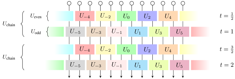
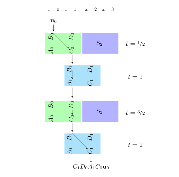
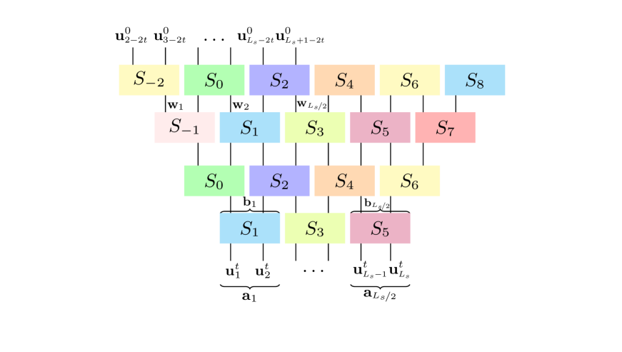
In this work we consider a spin chain with $L$ sites and periodic boundary conditions, where each site contains $N$ modes or qubits. The first dynamical period consists of two half-steps. In the first half-step each even site interacts with its right neighbour with a random Clifford unitary (for the definition of the Clifford group see Appendix A or Koenig and Smolin (2014)) and in the second half-step each odd site interacts with its right neighbour with a random Clifford unitary. These $L$ Clifford unitaries are independent and uniformly sampled from the $2N$-qubit Clifford group. The subsequent periods of the dynamics are repetitions of the first period, as illustrated in Figure 1. If we denote by $U_{x}$ the above-mentioned unitary action on sites $x$ and $x+1$ (modulo $L$ due to periodic boundary conditions) then the evolution operator after an integer time $t$ is

$$W(t) =\big{[}(U_{1}\otimes U_{3}\otimes\cdots\otimes U_{L-1})(U_{0}\otimes U_{2}\otimes\cdots\otimes U_{L-2})\big{]}^{t}$$ (1)

$$=(U_{\text{odd}}U_{\text{even}})^{t}=(U_{\text{chain}})^{t}\ ,$$

and after a half-integer time $t$ is

$$W(t)=U_{\text{even}}\,(U_{\text{chain}})^{t-1/2}\ .$$ (2)

This evolution operator can also be generated by a time-periodic Hamiltonian $H(t)$ with nearest-neighbour interactions

$$W(t)=\mathcal{T}e^{-\mathrm{i}\int_{0}^{t}d\tau H(\tau)}\ ,$$ (3)

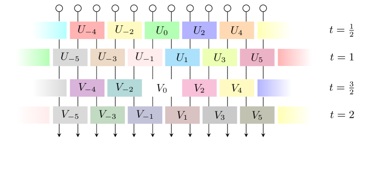
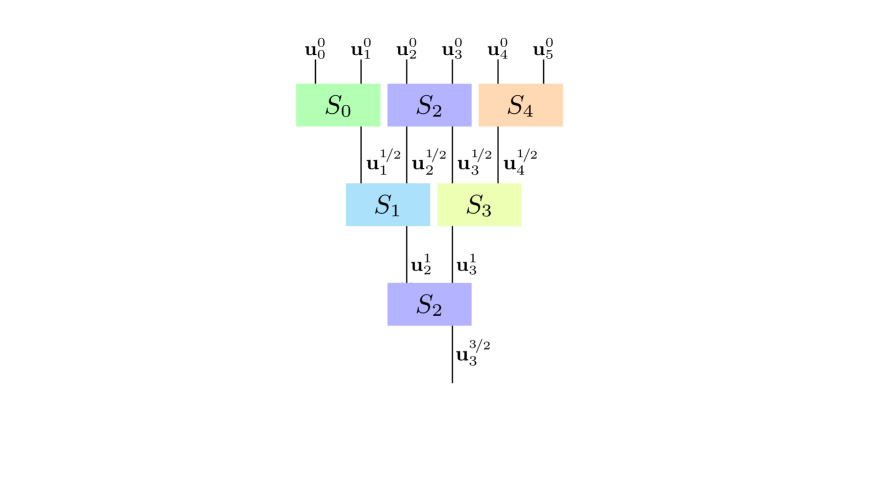
where $\mathcal{T}$ is the time-ordering operator. This type of dynamics is called Floquet. Floquet dynamics in relation with the phenomenon of quantum chaos has been studied, among others, by Prosen and coauthors Kos et al. (2018); Bertini et al. (2018, 2019, 2020), with the review Prosen (2007). A general review on quantum Floquet systems is reference Bukov et al. (2015). In the quantum information community the term QCA, quantum cellular automaton, commonly denotes such periodic systems Schlingemann et al. (2008), a review is Farrelly (2020). The authors of Sünderhauf et al. (2018) considered a QCA, with the same structure as us but with Haar-distributed unitaries gates instead of Cliffords. (Another Floquet-Clifford model has been studied in Chandran and Laumann (2015).) It is important to stress that this time-periodic model is very different from the much more studied time-dependent “random circuits” Harrow and Low (2009); Harrow and Mehraban (2018); Brandão et al. (2016a, b); Hunter-Jones (2019); Nakata et al. (2017); Brandão et al. (2021) depicted in Figure 2. Time-periodic circuits are more difficult to analyse but more relevant to physics; since they enjoy a (discrete) time translation symmetry.

Figure 2: Time-dependent local dynamics. In contrast to Figure 1 the pictured circuit is not periodic in time: different time steps are independently sampled.

We show that the ensemble of evolution operators at half-integer time (2) has a larger symmetry than that at integer times (1). This allows us to prove approximate Pauli mixing Webb (2016): each Pauli operator evolving with the random dynamics (2) reaches any other Pauli operator inside its light cone with approximately equal probability. In the integer-time case this only holds for a restricted class of initial operators, which includes local ones. We also prove that at any half-integer time after the scrambling time $t_{\rm scr}$, the ensemble of evolution operators (2) cannot be operationally distinguished from Haar-random unitaries (in the sense specified above). We define the scrambling time $t_{\rm scr}$ as the smallest time allowing for any local perturbation to reach the entire system (in our model $t_{\rm scr}=L/4$). In all these results, the degree of approximation increases with $N$ and decreases with time $t$.

Besides many-body physics, our results are relevant to the field of quantum information. The authors of Emerson et al. (2003) design a protocol to generate pseudo-random unitaries. Many quantum information tasks make use of unitary designs (entanglement distillation Bennett et al. (1996), quantum error correction Abeyesinghe et al. (2009); Brandão et al. (2016b), randomised benchmarking Magesan et al. (2011), quantum process tomography Scott (2008), quantum state decoupling Brown and Fawzi (2015) and data-hiding DiVincenzo et al. (2002)). In most current implementations of quantum information processing qubits are measured in a fixed basis, a particular case of our Pauli measurements. Hence we expect that our variant of 2-designs restricted to Pauli measurements will be useful in some of these applications, in particular on architectures where a time-periodic drive is more feasible than a time-dependent drive. It is worth mentioning that Google’s quantum supremacy demonstration Arute et al. (2019) is based on the statistics of multi-qubit Pauli measurements after pseudo-random unitary dynamics; and that their random circuit consists of time-dependent single-qubit gates and time-periodic two-qubit gates.

In the model under consideration, the number of modes per site $N$ is a free parameter that controls the behaviour of the system. In the large-$N$ regime ($N\gg\log L$) we obtain the above-mentioned indistinguishability between the evolution operator (2) and a Haar-random unitary, which increases with $N$. (We recall that large-$N$ is the relevant regime in holographic quantum gravity.) In the opposite regime ($N\ll\log L$) our model displays a novel form of localisation produced by the appearance of effective one-sided walls that prevent perturbations from crossing the wall in one direction but not the other. Interestingly, this localised phase seems to challenge the existing classification. On one hand, our model is not a system of free or interacting particles, so it does not fit in the framework of Anderson localisation. On the other hand, the evolution of each local operator is strictly confined to a finite region, so it does not behave as many-body localised. See Imbrie (2016) for the description of the differences among Anderson and many-body localisation and Nandkishore and Huse (2015) for a recent physicists’ review on localisation phenomena.

This model also challenges the classification of integrable and chaotic quantum systems. On one hand, it has a phase-space description of the dynamics like that of quasi-free bosons and fermions, and it can be efficiently simulated on a classical computer Aaronson and Gottesman (2004); Gottesman (1998). See reference Koenig and Smolin (2014) for an algorithmic classification of the elements of the Clifford group and appendix A for the description of the Clifford group phase space. On the other hand, this model does not have anything close to local (or low-weight) integrals of motions, and it behaves like Haar-random dynamics in a way that quasi-free systems do not. Therefore, we believe that Clifford dynamics is valuable for mapping the landscape of many-body phenomena. It is also important to recall that we live in the age of synthetic quantum matter, see the review Bloch et al. (2012), and models similar to ours have actually been implemented on quantum simulators, like in the recent Google’s experiment Arute et al. (2019).

In the following section we present our results on mixing (sections II.2 and II.3), pseudo-random unitaries (Section II.4) and strong localisation (Section II.5). In order to do so we introduce a few mathematical notions beforehand (Section II.1). The proofs of the theorems presented in the Section II are presented in sections V, V.2, V.3, V.4, VI, VII, together with several other lemmas. In Section VIII.1 we discuss the physical significance of the scrambling time. In Section VIII.2 we discuss the difficulties with classifying our model as integrable or chaotic. We compare time-periodic and time-independent circuits in Section VIII.3. In Section IX we provide the conclusions of our work. The appendices include an introduction to the Clifford formalism, appendix A, and some additional lemmas, appendix B and C.

II Results

II.1 Preliminaries

An $n$-qubit Pauli operator is a tensor product of Pauli sigma matrices and one-qubit identities times a global phase $\lambda\in\{1,\mathrm{i},-1,-\mathrm{i}\}$. In what follows we ignore this global phase $\lambda$, so each Pauli operator is represented by a binary vector ${\bf u}=(q_{1},p_{1},q_{2},p_{2},\ldots,q_{n},p_{n})\in\{0,1\}^{2n}$ as

$$\sigma_{\bf u}=\bigotimes_{i=1}^{n}(\sigma_{x}^{q_{i}}\sigma_{z}^{p_{i}})\ .$$ (4)

Ignoring the global phase $\lambda$ allows us to write the product of Pauli operators as the simple rule $\sigma_{\bf u}\sigma_{{\bf u}^{\prime}}=\lambda\,\sigma_{{\bf u}+{\bf u}^{\prime}}$, where addition in the vector space $\{0,1\}^{2n}$ is modulo 2. This defines the Pauli group, which is the discrete analog of the Weyl group, or the displacement operators used in quantum optics.

The $n$-qubit Clifford group $\mathcal{C}_{n}\subseteq{\rm SU}(2^{n})$ is the set of unitaries $U$ which map each Pauli operator onto another Pauli operator $U\sigma_{\bf u}U^{\dagger}=\lambda\,\sigma_{{\bf u}^{\prime}}$. Each Clifford unitary $U$ can be represented by a $2n\times 2n$ symplectic matrix $S$ with entries in $\{0,1\}$ such that its action on Pauli operators can be calculated in phase space

$$U\sigma_{\bf u}U^{\dagger}=\lambda\,\sigma_{S{\bf u}}\ ,$$ (5)

where the matrix product $S{\bf u}$ is defined modulo 2. We call the binary vectors ${\bf u}\in\{0,1\}^{2n}$ the phase space representation of the Pauli operator $\sigma_{\bf u}$ because of its analogy with quasi-free bosons, where dynamics is also linear and symplectic. A detailed introduction to the discrete phase space and Clifford and Pauli groups is provided in Appendix A, see also the references Koenig and Smolin (2014); Aaronson and Gottesman (2004); Gottesman (1998). Note that Clifford unitaries are easy to implement in several quantum computation and simulation architectures.

Our model is an $L$-site lattice with even $L$ and periodic boundary conditions. The corresponding phase space can be written as

$$\mathcal{V}_{\rm chain}=\bigoplus_{x\in\mathbb{Z}_{L}}\mathcal{V}_{x}\ ,$$ (6)

where $\mathcal{V}_{x}\cong\mathbb{Z}_{2}^{2N}$ is the phase space of site $x\in\mathbb{Z}_{L}$, which represents $N$ qubits. A local Pauli operator $\sigma_{\bf u}$ at site $x$ is represented by a phase-space vector contained in the corresponding subspace ${\bf u}\in\mathcal{V}_{x}\subseteq\mathcal{V}_{\rm chain}$. The identity operator corresponds to the zero vector. (See Section III for a collated description of the model and its phase space description). In the following we will denote $S(t)$ the symplectic matrix acting on the space $\mathcal{V}_{\rm chain}$ associated with the evolution operator $W(t)$ as defined by equations (1) and (2).

II.2 Approximate Pauli mixing

A set of unitaries $\mathcal{U}$ is Pauli mixing if a uniformly sampled unitary $U\in\mathcal{U}$ maps any non-identity Pauli operator $\sigma_{\bf u}$ to any other $\sigma_{{\bf u}^{\prime}}=U\sigma_{\bf u}U^{\dagger}$ with uniform distribution Webb (2016). Let us see that our model displays an approximate form of this property.

Each sequence of two-site Clifford unitaries $U_{0},\ldots,U_{L-1}$ defines an evolution operator $W(t)$ via equations (1-2), which maps each Pauli operator $\sigma_{\bf u}$ to another Pauli operator $\sigma_{{\bf u}^{\prime}}=\lambda W(t)\sigma_{\bf u}W(t)^{\dagger}$. This deterministic map ${\bf u}\mapsto{\bf u}^{\prime}$ becomes probabilistic when we let $U_{0},\ldots,U_{L-1}$ be random. In this case, the probability that ${\bf u}$ evolves onto ${\bf u}^{\prime}$ after a time $t$ is

$$P_{t}({\bf u}^{\prime}|{\bf u})=\mathop{\mathbb{E}}_{\{U_{x}\}}\left|2^{-NL}\tr(\sigma_{{\bf u}^{\prime}}W(t)\sigma_{{\bf u}}W(t)^{\dagger})\right|\ ,$$ (7)

where we use the orthogonality of Paulies $\tr(\sigma_{{\bf u}^{\prime}}\sigma_{{\bf u}})=2^{NL}\delta_{{\bf u}^{\prime}{\bf u}}$. The locality of the dynamics (see Figure 1) implies that only operators inside the light cone of the initial operator $\sigma_{\bf u}$ have non-zero probability (7). For example, if the initial operator $\sigma_{\bf u}$ is supported at the origin $x=0$, then after a time $t$, the evolved operator $\sigma_{{\bf u}^{\prime}}$ must be fully supported inside the light cone $-2t+1\leq x\leq 2t$. This means that the corresponding phase space vector ${\bf u}^{\prime}$ is in the causal subspace

$${\bf u}^{\prime}\in\bigoplus_{x\in[-2t+1,2t]}\mathcal{V}_{x}\ .$$ (8)

The time $t$ at which the causal subspace becomes the whole system is the scrambling time $t_{\rm scr}=L/4$. Section VIII.1 discusses the physical significance of this time scale.

When the distribution (7) is approximately uniform inside the light cone we say that the random dynamics displays approximate Pauli mixing. Let $Q_{t}({\bf u}^{\prime})$ denote the uniform distribution over all non-zero vectors ${\bf u}^{\prime}$ in the causal subspace (8), therefore after the scrambling time $t\geq t_{\rm scr}$, $Q_{t}({\bf u}^{\prime})$ is the uniform distribution over all non-zero vectors in the total phase space $\mathcal{V}_{\rm chain}$. The following theorem from Section V.3 proves approximate Pauli mixing for initially local operators.

Theorem 18 (Approximate Pauli mixing). If the initial Pauli operator $\sigma_{\bf u}$ is supported at site $x=0$ then the probability distribution (7) for its evolution $\sigma_{{\bf u}^{\prime}}$ is close to uniform inside the light cone, that is,

$$\sum_{{\bf u}^{\prime}}\left|P_{t}({\bf u}^{\prime}|{\bf u})-Q_{t}({\bf u}^{\prime})\right|\ \leq\ 130\times t^{2}\,2^{-N}\ ,$$ (9)

for any integer or half-integer time $t\in[1/2,2t_{\rm scr}]$. An analogous statement holds for any other initial location $x\neq 0$.

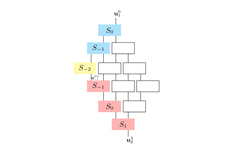
The above bound is useful in the large-$N$ limit ($N\gg\log t$). In the opposite regime ($N\ll\log L$) mixing cannot take place, since the system displays a strong form of localisation, in which local operators are mapped onto quasi-local operators. This phenomenon is illustrated in Figure 3 and detailed in Section II.5.

The error (9) increases with time due to time correlations and dynamical recurrences (see Section VIII.1). Hence, as time goes on the character of the system is less mixing, which is the opposite of what happens in time-dependent dynamics (see Section VIII.3). Also note that at integer times $t$ our model can be considered to be time-independent (instead of time-periodic) with discrete time.

The above mixing result only applies to local initial operators. Next, we present a different result that applies to a large class of non-local initial operators. However, due to the complexity of the problem, we only analyse their evolution inside a region $\mathcal{R}=\{1,\ldots,L_{\mathrm{s}}\}\subset\mathbb{Z}_{L}$.

Theorem 20. Consider an initial vector ${\bf u}^{0}\in\mathcal{V}_{\rm chain}$ with non-zero support in all lattice sites (${\bf u}_{x}^{0}\neq{\bf 0}$ for all $x\in\mathbb{Z}_{L}$). Consider the evolved vector ${\bf u}^{t}=S(t){\bf u}^{0}$ inside a region $x\in\{1,\ldots,L_{\mathrm{s}}\}\subseteq\mathbb{Z}_{L}$ where $L_{\mathrm{s}}$ is even and the time is $t\leq\frac{L-L_{\mathrm{s}}}{4}$. If ${\bf u}^{t}_{[1,Ls]}$ is the projection of ${\bf u}^{t}$ in the subspace $\bigoplus_{x=1}^{L_{\mathrm{s}}}\mathcal{V}_{x}$ then

$$\sum_{{\bf v}\in\mathbb{Z}_{2}^{2NL_{\mathrm{s}}}}\left|{\rm prob}\{{\bf v}={\bf u}^{t}_{[1,Ls]}\}-\frac{1}{2^{2NL_{\mathrm{s}}}}\right|\leq 32\,t\,2^{-N}(2L_{\mathrm{s}}+3^{\frac{L_{\mathrm{s}}}{2}+1})+4L2^{-2N}\ .$$ (10)

II.3 Pauli mixing at half-integer time

The evolution operator of our model $W(t)$ has an extra symmetry at half-integer time $t$ (see Section V.1). This allows us to prove a mixing result that is stronger than those of the previous section. Specifically, the following theorem (from Section V.2) applies to any initial Pauli operator instead of only local ones.

Theorem 14. Let $\sigma_{{\bf u}^{\prime}}=\lambda W(t)\sigma_{\bf u}W(t)^{\dagger}$ be the evolution of any initial Pauli operator $\sigma_{\bf u}\neq\mathbbm{1}$. At any half-integer time $t$ larger than the scrambling time, in the interval $t\in[t_{\rm scr},2t_{\rm scr}]$ the probability distribution (7) for the evolved operator $\sigma_{{\bf u}^{\prime}}$ is close to uniform, that is,

$$\sum_{{\bf u}^{\prime}}\left|P_{t}({\bf u}^{\prime}|{\bf u})-Q_{t}({\bf u}^{\prime})\right|\ \leq\ 33\times t\,L\,2^{-N}\ .$$ (11)

The fact that mixing is more prominent at half-integer multiples of the period is not restricted to Clifford dynamics, since it applies to a large class of periodic random quantum circuit or Floquet dynamics with disorder. In particular, it holds in any circuit where the two-site random interaction $U_{x}$ includes one-site random gates $V_{x}$ that are a 1-design. That is, when the random variable $U_{x}$ follows the same statistics than the random variable $U^{\prime}_{x}=U_{x}(V_{x}\otimes V_{x+1})$. This fact could be useful for implementing pseudo-random unitaries in quantum circuits with a periodic driving.

II.4 Pseudo-random unitaries

In this section we prove a consequence of the previous result: the evolution operator $W(t)$ at half-integer times $t$ is hard to physically distinguish from a Haar-random unitary $U\in{\rm SU}(2^{NL})$ when the available measurements are Pauli operators. More precisely, imagine that it is given a unitary transformation $V$ which has been sampled from either the set of evolution operators $\{W(t)\}$ or the full unitary group ${\rm SU}(2^{NL})$. The task is to choose a state $\rho$, process it with the given transformation $\rho\mapsto V\rho V^{\dagger}$, measure the result with a Pauli operator $\sigma_{\bf u}$, and guess whether $V$ has been sampled from the set of evolution operators $\{W(t)\}$ or from the full unitary group ${\rm SU}(2^{NL})$. In order to sharpen this discrimination procedure, two uses of the transformation $V$ are permitted, which allows for feeding each of them with half of an entangled state $\rho$ (describing two copies of the system). The following result tells us that, in the large-$N$ limit, the optimal guessing probability for the above task is almost as good as a random guess. (Recall that a random guess gives $p_{\rm guess}=1/2$). The proof is given in Section VI.

Theorem 21. Consider the task of discriminating between two copies of $W(t)$ and two copies of a Haar-random unitary $U$ with measurements restricted to Pauli operators, when $t\in[t_{\rm scr},2t_{\rm scr}]$ is half-integer. The success probability for correctly guessing the given pair of unitaries satisfies

$$p_{\rm guess}=\ \frac{1}{2}+\frac{1}{4}\ \max_{\rho,{\bf u},{\bf v}}\ \tr\!\left(\!\sigma_{\bf u}\otimes\sigma_{\bf v}\!\left[\mathop{\mathbb{E}}_{W(t)}W(t)^{\otimes 2}\rho\,W(t)^{\otimes 2\dagger}-\int_{{\rm SU}(d)}dU\,U^{\otimes 2}\rho\,U^{\otimes 2\dagger}\right]\right)$$

$$\leq\ 1/2+9\,tL2^{-N}\ .$$ (12)

The proof that the optimal guessing probability is given by formula (12) can be found in Nielsen and Chuang (2010). If in Theorem 21, measurements were not restricted then $W(t)$ would be an $(8\,tL2^{-N})$-approximate unitary 2-design. The precise definition of approximate 2-design allows for using an ancillary system in the discrimination process Gross et al. (2007). However, we have not included this ancillary system in Theorem 21 because it does not provide any advantage.

II.5 Strong localisation ($N\ll\log L$)

The model under consideration has the property that certain combinations of gates in consecutive sites (e.g. $U_{x},U_{x+1},\ldots,U_{x+l}$) generate right- or left-sided walls. These are defined as follows: a right-sided wall at site $x$ stops the growth towards the right of any operator that arrives at $x$ from the left, but it does not necessarily stop the growth towards the left of any operator that arrives at $x$ from the right. The analogous thing happens for left-sided walls (see Figure 3).

These gate configurations have a non-zero probability, hence, they will appear in a sufficiently long chain with a typical circuit. Below we provide bounds to this probability. The inverse of this probability is the average distance between walls, which can be understood as the localisation length scale, and it quantifies the width of the lightcones displayed in Figure 3.

Figure 3: Strong localisation. This figure displays the Heisenberg evolution of the initial operator $\sigma_{z}$ at site $x=1$. Each lattice site consists of one qubit ($N=1$) with first-neighbour interactions. After a phase of linear growth the lateral wings collide with left- and right-sided walls with penetration length $l=1$, that confine the evolution for all times. This confinement affects all (not necessarily local or Pauli) operators between the two walls. Inside the confined region evolution seems to be mixing.

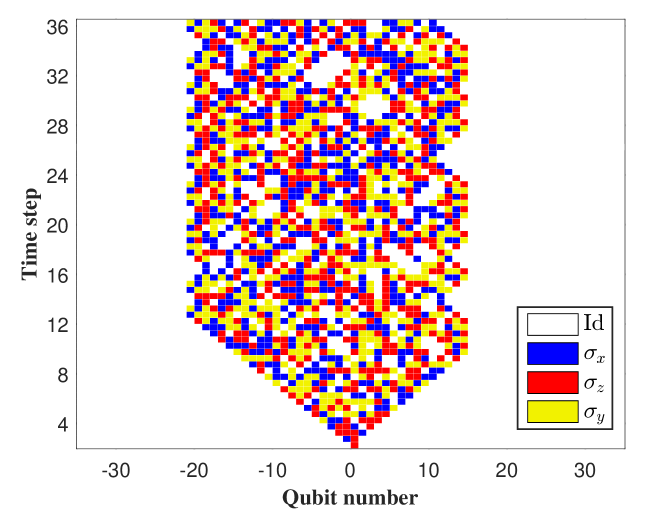
Each one-sided wall has some penetration length $l\geq 1$ into the forbidden region. Suppose that a realisation of $U_{\rm chain}$ contains a right-sided wall at site $x=0$ with penetration length $l$. Then any operator with support on the sites $x\leq 0$ (and identity on $x>0$) is mapped by $(U_{\rm chain})^{t}$ to an operator with support on $x\leq l$ contained in a specific subspace within the interval $x\in[1,l]$ such that entering into region $x>l$ is impossible for all $t\geq 1$. (The restriction to this subspace within the forbidden region can be seen in Figure 3 (with $l=1$) by the fact that the right-most points are either yellow followed by red, or white followed by white. And the left-most points are either blue followed by yellow, or white followed by white.) An initial operator with support on the interval $x\in[1,l]$ which does not have the specific structure mentioned above can pass through and reach the side $x>l$.

Now let us characterize the pairs of gates $U_{0},U_{1}$ (which act on sites $\{0,1\}$ and $\{1,2\}$ respectively) that generate a right-sided wall at $x=0$ with penetration length $l\leq 1$. Let $S_{0},S_{1}$ be the phase-space representation of $U_{0},U_{1}$. Next we use the fact that in phase space subsystems decompose with the direct sum (not the tensor product) rule, which allows to decompose $S_{0},S_{1}$ in $2N$-dimensional blocks

$$S_{x}=\left(\begin{array}[]{cc}A_{x}&B_{x}\\ C_{x}&D_{x}\end{array}\right)\ .$$ (13)

The flow of information caused by $S_{x}$ is easily seen by the action of $S_{x}$ on the vector $({\bf u}_{x},{\bf u}_{x+1})^{T}$:

$$\left(\begin{array}[]{cc}A_{x}&B_{x}\\ C_{x}&D_{x}\end{array}\right)\ \left(\begin{array}[]{cc}{\bf u}_{x}\\ {\bf u}_{x+1}\end{array}\right)\ =\left(\begin{array}[]{cc}A_{x}{\bf u}_{x}+B_{x}{\bf u}_{x+1}\\ C_{x}{\bf u}_{x}+D_{x}{\bf u}_{x+1}\end{array}\right)\$$ (14)

Block $A_{0}$ ($D_{0}$) represents the local dynamics at site $x=0$ ($x=1$) in the first half step. Block $C_{0}$ represents the flow from $x=0$ to $x=1$ in the first half step, and block $C_{1}$ represents the flow from $x=1$ to $x=2$ in the second half step.

Figure 4: The flow of information starting from $x=0$ at $t=0$ shows that with $C_{1}C_{0}=0$ there is no information reaching $x=2$ at $t=1$.

Figure 5: As illustrated in Figure 4, the condition $C_{1}C_{0}=0$ stops the information flow from $x=0$ at $t=0$ to $x=2$ at $t=1$. To prevent this from happening also at $t=2$ we demand that $C_{1}D_{0}A_{1}C_{0}=0$.

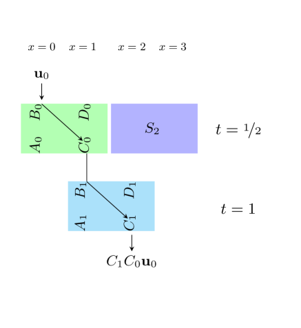
Imposing that nothing arrives at $x=2$ after the first whole step amounts to $C_{1}C_{0}=0$. This is illustrated in Figure 4. Imposing that nothing arrives at $x=2$ after the first two whole steps amounts to

$$C_{1}D_{0}A_{1}C_{0}=0\ \mbox{ and }\ C_{1}C_{0}=0\ .$$ (15)

This is illustrated in Figure 5. Finally, imposing that nothing arrives at $x=2$ after any number $(t+1)$ of whole steps amounts to

$$C_{1}(D_{0}A_{1})^{t}C_{0}=0\,,$$ (16)

for all integers $t\geq 0$. However, it is proven in Lemma 24 (Section VII) that this infinite family of conditions (16) is implied by the cases $t=0,1,\ldots,(2^{4N}-1)$. And for the simplest case $N=1$, Theorem 25 shows that all conditions (16) follow from the two conditions (15).

Equations (15) and (16) can be understood as characterising a pattern of destructive interference due to disorder which causes localisation.

The following pair of Clifford unitearies $U_{0},U_{1}$

$$U_{0}=\frac{1}{\sqrt{2}}\begin{pmatrix}i&0&0&-i\\ 0&i&-i&0\\ 1&0&0&1\\ 0&1&1&0\\ \end{pmatrix},\ \ \ \ U_{1}=\frac{1}{2}\begin{pmatrix}1&-1&1&1\\ -1&1&1&1\\ 1&1&1&-1\\ 1&1&-1&1\\ \end{pmatrix},$$ (17)

has phase-space representation

$$S_{0}=\begin{pmatrix}1&1&0&1\\ 0&1&0&1\\ 1&0&1&0\\ 0&0&0&1\\ \end{pmatrix},\ \ \ \ S_{1}=\begin{pmatrix}1&0&0&1\\ 0&1&0&0\\ 0&1&1&0\\ 0&0&0&1\\ \end{pmatrix}.$$ (18)

It can be checked that this pair of matrices satisfies conditions (15), which implies (16).

The following theorem provides the exact value of the probability for the appearance of a one-sided wall with penetration length $l=1$, in the case $N=1$.

Theorem 25. For $N=1$ the conditions

$$C_{x+1}\left(D_{x}A_{x+1}\right)^{k}C_{x}=0,$$ (19)

for $k\in\{0,1,2,\ldots\}$ are implied by the two conditions

$$C_{x+1}C_{x}=0\quad\text{ and }\quad C_{x+1}D_{x}A_{x+1}C_{x}=0\ .$$ (20)

Furthermore the probability of this is given exactly by

$${\rm prob}\{C_{x+1}C_{x}=0,C_{x+1}D_{x}A_{x+1}C_{x}=0\}=0.12\ \ ,$$ (21)

which includes trivial localisation.

The probability given in equation (21) is obtained numerically. It is worth mentioning that this model also displays walls with zero penetration length ($l=0$), which are necessarily two-sided. These walls happen when a two-site gate $U_{x}$ is of product form $U_{x}=V_{x}\otimes V_{x+1}$. This prevents the interaction between the two sides of the gate, and hence, it produces a trivial type of localisation. The following theorem (proven in Section VII) shows that the probability of these trivial walls is very small.

Theorem 23 The probability that a Clifford unitary $U\in\mathcal{C}_{2N}$ is of product form is

$$\frac{1}{2}\,2^{-4N^{2}}\leq{\rm prob}\{U\ {\rm is\ product}\}\leq 2^{-4N^{2}}\ .$$ (22)

We expect that $(l=0)$-walls are much less likely, except in the case $N=1$, than $(l\geq 1)$-walls. This would allow for a regime of $(L,N)$ where the system displays non-trivial localisation.

II.6 Absence of localisation ($N\gg\log L$)

The following theorem provides an upper bound for the probability that one-sided walls appear at a particular location. This upper bound implies that when $N\gg\log L$ a typical circuit has no localisation.

Theorem 27. The conditions

$$C_{x+1}\left(D_{x}A_{x+1}\right)^{k}C_{x}=0\ \ \mbox{ for all }\ \ k\in\{0,1,2,\ldots\}\ ,$$ (23)

are sufficient to prevent all right-wards propagation past position $x$ at any time. The probability that this family of constrains holds is upper-bounded by

$${\rm prob}\{C_{x+1}\left(D_{x}A_{x+1}\right)^{k}C_{x}=0,\ \forall k\in\mathbb{N}\}$$

$$\leq\ {\rm prob}\{C_{x+1}C_{x}=0\}\ \leq\ \frac{2N+1}{(1-2^{-2N})^{2N}}\,2^{2N-2N^{2}}.$$ (24)

By symmetry, left-sided walls have the same probabilities.

If the system is finite ($L<\infty$), a sufficiently large $N$ will eliminate the presence of localisation in most realisations of the dynamics $U_{\rm chain}$. This fact is crucial in the mixing results of the previous sections. Our previous results showing the mixing property in the regime $N\gg\log L$, suggest that in this regime the probability that the whole system has a wall of any type vanishes.

III Description of the model

In this section we further specify the model analysed in this work.

III.1 Locality, time-periodicity and disorder

Consider a spin chain with an even number $L$ of sites and periodic boundary conditions. Each site is labeled by $x\in\mathbb{Z}_{L}$ and contains $N$ qubits (Clifford modes), so the Hilbert space of each site has dimension $2^{N}$. The dynamics of the chain is discrete in time, and hence, it is characterised by a unitary $U_{\rm chain}$, not a Hamiltonian. Locality is imposed by the fact that $U_{\rm chain}$ is generated by first-neighbour interactions in the following way

$$U_{\rm chain}=\left(\mbox{$\bigotimes_{x{\rm\,odd}}$}U_{x}\right)\left(\mbox{$\bigotimes_{x{\rm\,even}}$}U_{x}\right)$$ (25)

where the unitary $U_{x}$ only acts on sites $x$ and $x+1$ ($\bmod L$ is understood). The expression (25) tells us that each time step decomposes in two half steps: in the first half each even site interacts with its right neighbor, and in the second half each even site interacts with its left neighbor. This is illustrated in Figure 1.

We define the evolution operator at integer and half-integer times $t\in\mathbb{Z}/2$ in the following way

$$W(t)=\left\{\begin{array}[]{ll}(U_{\rm chain})^{t}&\ \mbox{integer $t$}\\ (\mbox{$\bigotimes_{x{\rm\,even}}$}U_{x})(U_{\rm chain})^{t-1/2}&\ \mbox{half-integer $t$}\end{array}\right.\ .$$ (26)

We understand that $t$ is half-integer when $t-1/2\in\mathbb{Z}$.

Translation invariance amounts to imposing that all $U_{x}$ with even $x$ are identical, and all $U_{x}$ with odd $x$ are identical too. However, in this work we are interested in disordered systems, where the translation invariance is broken. In fact, here we break the translation invariance in the strongest possible form, since each two-site unitary $U_{x}$ is independently sampled from the uniform distribution over the Clifford group.

III.2 Phase-space description

The phase space of the whole chain is

$$\mathcal{V}_{\rm chain}=\mbox{$\bigoplus_{x}$}\mathcal{V}_{x}\cong\mathbb{Z}_{2}^{2NL}\ ,$$ (27)

where $\mathcal{V}_{x}\cong\mathbb{Z}_{2}^{2N}$ is the phase space of site $x$. The phase-space representation of $U_{x}$ is the symplectic matrix $S_{x}\in\mathcal{S}_{2N}$, where $S_{x}$ acts on the subspace $\mathcal{V}_{x}\oplus\mathcal{V}_{x+1}$. Using this direct-sum decomposition we can write

$$S_{x}=\left(\begin{array}[]{cc}A_{x}&B_{x}\\ C_{x}&D_{x}\end{array}\right)\ ,$$ (28)

where $A_{x},B_{x},C_{x},D_{x}$ are $2N\times 2N$ matrices, with $A_{x}:\mathcal{V}_{x}\rightarrow\mathcal{V}_{x}$, $B_{x}:\mathcal{V}_{x+1}\rightarrow\mathcal{V}_{x}$, $C_{x}:\mathcal{V}_{x}\rightarrow\mathcal{V}_{x+1}$, $D_{x}:\mathcal{V}_{x+1}\rightarrow\mathcal{V}_{x+1}$. The phase-space representation of $U_{\rm chain}$ given in (25) is

$$S_{\rm chain}=\left(\mbox{$\bigoplus_{x\,{\rm odd}}$}S_{x}\right)\left(\mbox{$\bigoplus_{x\,{\rm even}}$}S_{x}\right)\ .$$ (29)

Note that the tensor product becomes a direct sum, in analogy with the quantum optics formalism. Using the single-site decomposition (27) and (28) we can write the two half steps in (29) as

$$\bigoplus_{x\,{\rm even}}\mathcal{S}_{x} =\left(\begin{array}[]{ccccccc}A_{0}&B_{0}&&&&&\\ C_{0}&D_{0}&&&&&\\ &&A_{2}&B_{2}&&&\\ &&C_{2}&D_{2}&&&\\ &&&&\ddots&&\\ &&&&&A_{L-2}&B_{L-2}\\ &&&&&C_{L-2}&D_{L-2}\\ \end{array}\right),$$ (37)

$$\bigoplus_{x\,{\rm odd}}\mathcal{S}_{x} =\left(\begin{array}[]{ccccccc}D_{L-1}&&&&&&C_{L-1}\\ &A_{1}&B_{1}&&&&\\ &C_{1}&D_{1}&&&&\\ &&&\ddots&&&\\ &&&&A_{L-3}&B_{L-3}&\\ &&&&C_{L-3}&D_{L-3}&\\ B_{L-1}&&&&&&A_{L-1}\\ \end{array}\right),$$ (45)

where the blank spaces represent blocks with zeros. The “phase space evolution operator” is then

$$S(t)=\left\{\begin{array}[]{ll}(S_{\rm chain})^{t}&\ \mbox{integer $t$}\\ (\mbox{$\bigoplus_{x{\rm\,even}}$}S_{x})(S_{\rm chain})^{t-1/2}&\ \mbox{half-integer $t$}\end{array}\right.\ .$$ (46)

IV Random symplectic matrices

In this section we discuss results relating to (uniformly) random symplectic matrices. These results will then be used in the Section V to show that the random local circuit model we consider approximately satisfies the requirement of Pauli mixing: it maps any initial Pauli operator to the uniform distribution over all Pauli operators.

An equivalent way to write the symplectic condition $S^{T}JS=J$ is that the columns of the matrix $S=({\bf u}_{1},{\bf v}_{1},{\bf u}_{2},{\bf v}_{2},\ldots,{\bf u}_{n},{\bf v}_{n})$ satisfy

$$\langle{\bf u}_{i},{\bf u}_{j}\rangle=\langle{\bf v}_{i},{\bf v}_{j}\rangle =0\ ,$$ (47)

$$\langle{\bf u}_{i},{\bf v}_{j}\rangle =\delta_{ij}\ .$$ (48)

We recall the notation $\langle{\bf r},{\bf s}\rangle\equiv{\bf r}^{T}J{\bf s}$, for all ${\bf r},{\bf s}\in\mathbb{Z}_{2}^{2n}$. Using this, we can uniformly sample from $\mathcal{S}_{n}$ by sequentially generating the columns of $S$.

Lemma 1.

The following algorithm allows to uniformly sample from the symplectic group $\mathcal{S}_{n}$.

1. Generate ${\bf u}_{1}$ by picking any of the $(2^{2n}-1)$ non-zero vectors in $\mathbb{Z}_{2}^{2n}$.

2. Generate ${\bf v}_{1}$ by picking any of the $2^{2n-1}$ vectors satisfying $\langle{\bf u}_{1},{\bf v}_{1}\rangle=1$.

3. Generate ${\bf u}_{2}$ by picking any of the $(2^{2n-2}-1)$ non-zero vectors satisfying $\langle{\bf u}_{1},{\bf u}_{2}\rangle=\langle{\bf v}_{1},{\bf u}_{2}\rangle=0$.

4. Generate ${\bf v}_{2}$ by picking any of the $2^{2n-3}$ vectors satisfying $\langle{\bf u}_{1},{\bf v}_{2}\rangle=\langle{\bf v}_{1},{\bf v}_{2}\rangle=0$ and $\langle{\bf u}_{2},{\bf v}_{2}\rangle=1$.

5. Continue generating ${\bf u}_{3},{\bf v}_{3},\ldots,{\bf u}_{n},{\bf v}_{n}$ in analogous fashion, completing the matrix $S=({\bf u}_{1},{\bf v}_{1},{\bf u}_{2},{\bf v}_{2},\ldots,{\bf u}_{n},{\bf v}_{n})$.

Proof.

We first look at the number of vectors $({\bf u}_{1},{\bf v}_{1},{\bf u}_{2},{\bf v}_{2},\ldots,{\bf u}_{n},{\bf v}_{n})$, as stated above, that ensures $S$ symplectic.

${\bf v}_{1}$ has $2n$ components, since there is one constraint, the number of independent components is $2n-1$, each component belongs to $\mathbb{Z}_{2}$, therefore the number of vectors ${\bf v}_{1}$ equals $2^{2n-1}$. Notice that since ${\bf u}_{1}$ is non vanishing, a vanishing ${\bf v}_{1}$ cannot solve $\langle{\bf u}_{1},{\bf v}_{1}\rangle=1$.

${\bf u}_{2}$ must satisfy two constraints, the number of independent components is $2n-2$, then there are $2^{2n-2}$ solutions, this includes also the case that ${\bf u}_{2}$ is vanishing, but since $S$ must be full rank we need to exclude it, therefore there are $2^{2n-2}-1$ admissible ${\bf u}_{2}$ vectors. And so on.

We now proof that the distribution of simplectic matrices $S$ generated with the algorithm is uniform. Let us see that the number of symplectic matrices whose first column is the non-zero vector ${\bf u}_{1}$ is independent of ${\bf u}_{1}$.

1. The number of vectors ${\bf v}_{1}$ satisfying $\langle{\bf u}_{1},{\bf v}_{1}\rangle=1$ is independent of which non-zero ${\bf u}_{1}$ we choose.

2. The number of vectors ${\bf u}_{2}$ satisfying $\langle{\bf u}_{1},{\bf u}_{2}\rangle=1$ and $\langle{\bf u}_{2},{\bf v}_{1}\rangle=0$ is independent of the pair ${\bf u}_{1},{\bf v}_{1}$ (being both non-zero and $\langle{\bf u}_{1},{\bf v}_{1}\rangle=1$) that we choose.

3. And analogously for ${\bf v}_{2},{\bf u}_{3}$, and so on.

This shows that the number of matrices having a fixed first column ${\bf u}_{1}$ is independent of ${\bf u}_{1}$. Therefore, all first columns ${\bf u}_{1}$ need to have the same probability. Using the steps 1,2,3 in a similar fashion we can analogously conclude that all second columns ${\bf v}_{1}$ need to have the same probability. And analogously, all vectors for column $k$ (compatible with columns $1,2,...,k-1$) need to have the same probability. This shows the uniformity provided by the sampling algorithm of Lemma 6.

∎

To obtain the above numbers, we use the fact that when $\langle{\bf u},{\bf v}\rangle=1$ both, ${\bf u}$ and ${\bf v}$, are non-zero. From these same numbers the next result follows.

Lemma 2.

The order of the symplectic group is

$$|\mathcal{S}_{n}|=(2^{2n}-1)2^{2n-1}(2^{2n-2}-1)2^{2n-3}\cdots(2^{2}-1)2^{1}\ ,$$ (49)

and it satisfies

$$a(n)\,2^{2n^{2}+n}\ \leq\ |\mathcal{S}_{n}|\ \leq\ b(n)\,2^{2n^{2}+n}\$$ (50)

with $0.64<a(n)<b(n)<0.78$.

The proof of (49) is a classic result to be found for example in Artin (1957), it also directly follows from Lemma 1. The proof of equation (50) is in the appendix B.

Finally, the next Lemma shows that uniformly distributed symplectic matrices have random outputs.

Lemma 3 (Uniform output).

If $S\in\mathcal{S}_{n}$ is uniformly distributed, then for any pair of non-zero vectors ${\bf u},{\bf u}^{\prime}\in\mathbb{Z}_{2}^{2n}$ we have

$${\rm prob}\{{\bf u}^{\prime}=S{\bf u}\}=(2^{2n}-1)^{-1}\ .$$ (51)

Proof.

Let us first consider the case ${\bf u}=(1,0,\ldots,0)^{T}$. If we follow the algorithm of Lemma 1, then the image of $(1,0,\ldots,0)^{T}$ is uniformly distributed over the $(2^{2n}-1)$ non-zero vectors, and hence, it follows (51). To show (51) for any given ${\bf u}$, take any $S_{0}\in\mathcal{S}_{n}$ such that $S_{0}{\bf u}=(1,0,\ldots,0)^{T}$, and note that, if $S$ is uniformly distributed then so is $SS_{0}$. ∎

IV.1 Rank of sub-matrices of $S$

Lemma 4.

Any given $S\in\mathcal{S}_{2n}$ can be written in block form

$$S=\left(\begin{array}[]{cc}A&B\\ C&D\end{array}\right),$$ (52)

according to the local decomposition $\mathbb{Z}_{2}^{4n}=\mathbb{Z}_{2}^{2n}\oplus\mathbb{Z}_{2}^{2n}$. If $S$ is uniformly distributed this then induces a distribution on the sub-matrices $A,B,C,D$. For each of them ($E=A,B,C,D$) the induced distribution satisfies

$${\rm prob}\big{\{}{\rm rank}\,E\leq 2n-k\big{\}}\ \leq\ \min\{2^{k},4\}\frac{2^{-k^{2}}}{(1-2^{-2n})^{k}}\approx 4\times 2^{-k^{2}}\ .$$ (53)

Proof.

We proceed by studying the rank of $C$ and later generalizing the results to $A,B,D$. Equation (53) is trivial for $k=0$, so in what follows we assume $k\geq 1$. Let us start by counting the number of matrices $S\in\mathcal{S}_{2n}$ with a sub-matrix $C$ satisfying $C{\bf u}={\bf 0}$ for a given (arbitrary) non-zero vector ${\bf u}\in\mathbb{Z}_{2}^{2n}$. Let $r$ denote the position of the last “1” in ${\bf u}$, so that it can be written as:

$${\bf u}=\big{(}\underbrace{{\bf u}^{1},\ldots,{\bf u}^{r-1}}_{r-1},1,\underbrace{0,\ldots,0}_{2n-r}\big{)}^{T}\ ,$$ (54)

where ${\bf u}^{1},\ldots,{\bf u}^{r-1}\in\{0,1\}$. Then, the constraint $C{\bf u}={\bf 0}$ can be written as

$$\begin{cases}C_{i,1}=0,\hskip 14.22636pt\textrm{if}\,r=1,\hskip 14.22636pt\textrm{with}\,1\leq i\leq 2n\\ C_{i,r}=\sum_{j=1}^{r-1}C_{i,j}\,{\bf u}^{j},\hskip 14.22636pt\textrm{if}\,r>1,\hskip 14.22636pt\textrm{with}\,1\leq i\leq 2n\end{cases}$$ (55)

where $C_{i,j}$ are the components of $C$. (55) reads as a constraint on the $r$-th column of the matrix $C$.

Next, we follow the algorithm introduced in Lemma 1 for generating a matrix $S\in\mathcal{S}_{2n}$ column by column, from left to right, and in addition to the symplectic constraints we include (55). Constraint (55) can be imposed by ignoring it during the generation of columns $1,\ldots,r-1$, completely fixing the rows $2n<i\leq 4n$ of the $r$ column, that corresponds to the $r$-th column of the matrix $C$, and again ignoring it during the generation of columns $r+1,\ldots,4n$. By counting as in Lemma 2 we obtain that the number of matrices $S\in\mathcal{S}_{2n}$ satisfying $C{\bf u}={\bf 0}$ follows

$$|\{S\in\mathcal{S}_{2n}:C{\bf u}={\bf 0}\}|$$ (56)

$$\leq\begin{cases}(2^{4n}-1)(2^{4n-1})\cdots(2^{4n-(r-2)}-1)2^{2n-(r-1)}(2^{4n-r}-1)\cdots 2^{1},\hskip 8.53581pt\textrm{r even}\\ (2^{4n}-1)(2^{4n-1})\cdots 2^{4n-(r-2)}2^{2n-(r-1)}2^{4n-r}\cdots 2^{1},\hskip 8.53581pt\textrm{r odd}\end{cases}$$

.

Equation (56) is an inequality because, for some values of the first $r-1$ columns of $S$ and the $r$-th column of $C$, it is impossible to complete the $r$-th column of $A$ satisfying the symplectic constraints (47-48).

The probability that a random $S$ satisfies $C{\bf u}={\bf 0}$ is

$${\rm prob}\{C{\bf u}={\bf 0}\}=\frac{|\{S\in\mathcal{S}_{2n}:C{\bf u}={\bf 0}\}|}{|\mathcal{S}_{2n}|}\ .$$ (57)

By noting that all factors in (56) are the same as in (49) except for the factor at position $r$, we obtain

$${\rm prob}\{C{\bf u}={\bf 0}\} \leq\frac{2^{2n-(r-1)}}{2^{4n-(r-1)}-\alpha^{\prime}}\leq\frac{2^{2n-(r-1)}}{2^{4n-(r-1)}-1}$$

$$=\frac{2^{-2n}}{1-2^{(r-1)-4n}}\leq\frac{2^{-2n}}{1-2^{-2n}}\ ,$$ (58)

where $\alpha^{\prime}=1$ if $r$ is odd and $\alpha^{\prime}=0$ otherwise. The last inequality above follows from $r\leq 2n$. The bound (58) is correct also for $r=1$. The fact that bound (58) is independent of $r$ is crucial for the rest of the proof.

Next, we generalize bound (58) to the case where $C{\bf u}_{i}=0$ for $k$ given linearly-independent vectors ${\bf u}_{i}\in\{{\bf u}_{1},\dots,{\bf u}_{k}\}$. To do this, we take the $2n\times k$ matrix $[{\bf u}_{1},\dots,{\bf u}_{k}]$ and perform Gauss-Jordan elimination, operating on the columns, to obtain a matrix $[{\bf v}_{1},\dots,{\bf v}_{k}]$ having column-echelon form. $\{C{\bf u}_{1}={\bf 0},\ldots,C{\bf u}_{k}={\bf 0}\}$ is equivalent to $\{C{\bf v}_{1}={\bf 0},\ldots,C{\bf v}_{k}={\bf 0}\}$, in fact only two operations are performed on the set $\{{\bf u}_{1},\ldots,{\bf u}_{k}\}$ to obtain the set $\{{\bf v}_{1},\ldots,{\bf v}_{k}\}$: changing the order of the vectors $\{{\bf u}_{1},\ldots,{\bf u}_{k}\}$, replacing a vector ${\bf u}_{j}$ with the sum of ${\bf u}_{j}$ with another vector ${\bf u}_{l}$. If we denote by $r_{i}$ the position of the last “1” of ${\bf v}_{i}$, then column-echelon form amounts to $r_{1}<r_{2}<\cdots<r_{k}$. Now we proceed as above to generate each column of $S$ satisfying the symplectic and the $C{\bf v}_{i}={\bf 0}$ constraints. This gives

$${\rm prob}\{C{\bf u}_{1}={\bf 0},\ldots,C{\bf u}_{k}={\bf 0}\}\leq\frac{2^{2n-(r_{1}-1)}}{2^{4n-(r_{1}-1)}-\alpha^{\prime}_{1}}\frac{2^{2n-(r_{2}-1)}}{2^{4n-(r_{2}-1)}-\alpha^{\prime}_{2}}\cdots\frac{2^{2n-(r_{k}-1)}}{2^{4n-(r_{k}-1)}-\alpha^{\prime}_{k}}\ ,$$ (59)

where $\alpha^{\prime}_{i}\in\{0,1\}$. Similarly as in (58) we obtain

$${\rm prob}\{C{\bf u}_{1}={\bf 0},\ldots,C{\bf u}_{k}={\bf 0}\}\leq\frac{2^{-2nk}}{(1-2^{-2n})^{k}}\ .$$ (60)

If we multiply the above bound by the number $\mathcal{N}_{k}^{2n}$ of $k$-dimensional subspaces of $\mathbb{Z}_{2}^{2n}$ (see appendix C), then we obtain

$${\rm prob}\{\text{rank}(C)\leq 2n-k\} =\mathcal{N}_{k}^{2n}\ {\rm prob}\{C{\bf u}_{1}={\bf 0},\ldots,C{\bf u}_{k}={\bf 0}\}$$

$$\leq\min\{2^{k},4\}\,\frac{2^{2nk}}{2^{k^{2}}}\,\frac{2^{-2nk}}{(1-2^{-2n})^{k}}\ ,$$

$$=\min\{2^{k},4\}\,\frac{2^{-k^{2}}}{(1-2^{-2n})^{k}}\ ,$$ (61)

where in the last inequality we used Lemma 34. Using Lemma 36 (appendix C), the above argument applies to any of the four sub-matrices $A,B,C,D$. The proof of equation (53) is then completed. ∎

IV.2 Rank of product of sub-matrices

Lemma 5.

Let the random matrices $S_{1},S_{2},\ldots,S_{r}\in\mathcal{S}_{2n}$ be independent and uniformly distributed, which induces a distribution for the sub-matrices

$$S_{i}=\left(\begin{array}[]{cc}A_{i}&B_{i}\\ C_{i}&D_{i}\end{array}\right).$$ (62)

For any choice $E_{i}\in\{A_{i},B_{i},C_{i},D_{i}\}$ for each $i\in\{1,\ldots,r\}$, we have

$${\rm prob}\big{\{}{\rm rank}(E_{r}\cdots E_{1})\leq 2n-k\} \leq\ \frac{2^{k}}{(1-2^{-2n})^{k}}\binom{k+r-1}{k}2^{-\frac{1}{2}k^{2}}\ .$$ (63)

Proof.

Before analyzing the rank of the product of $r$ independent random matrices $C_{r}\cdots C_{1}$, we start by a much simpler problem. Analyzing the rank of the product $CF$ where $C$ follows the usual $C$-distribution and $F$ is a fixed $2n\times 2n$ matrix with ${\rm rank}(F)=2n-k_{1}$. Noting that the input space of $C$ has dimension $2n-k_{1}$, from (IV.1), with $k_{2}\equiv k-k_{1}\geq 0$, we obtain

$${\rm prob}\big{\{}{\rm rank}(CF)\leq 2n-k\big{\}} \leq\mathcal{N}_{k_{2}}^{2n-k_{1}}{\rm prob}\{C{\bf u}_{1}={\bf 0},\ldots,C{\bf u}_{k_{2}}={\bf 0}\}$$

$$\leq\min\{2^{k_{2}},4\}\,\frac{2^{(2n-k_{1})k_{2}}}{2^{k_{2}^{2}}}\,\frac{2^{-2nk_{2}}}{(1-2^{-2n})^{k_{2}}}$$

$$\leq\frac{2^{k_{2}-k_{1}k_{2}-k_{2}^{2}}}{(1-2^{-2n})^{k_{2}}}\ ,$$ (64)

Proceeding in a similar fashion, we can analyze the product of two independent $C$-matrices. To do so, we multiply two factors (64) and sum over all possible intermediate kernel sizes $k_{1}$, obtaing

$${\rm prob}\big{\{}{\rm rank}(C_{2}C_{1})\leq 2n-k\big{\}} \leq\sum_{k_{1}=0}^{k}\frac{2^{k_{2}-k_{2}k_{1}-k_{2}^{2}}}{(1-2^{-2n})^{k_{2}}}\ \frac{2^{k_{1}-k_{1}^{2}}}{(1-2^{-2n})^{k_{1}}}$$ (65)

$$=\sum_{k_{1}=0}^{k}\frac{2^{k-k_{2}k_{1}-k_{1}^{2}-k_{2}^{2}}}{(1-2^{-2n})^{k}},$$

where again $k_{2}=k-k_{1}$.

Equation (65) works as follows: the matrix $F$ in (64) has fix rank equal to $2n-k_{1}$. That’s the dimension of the input space of $C$. In (65) the input space of $C_{1}$ is the full space $\mathbb{Z}_{2}^{2n}$ that has dimension $2n$, therefore the factor $\frac{2^{k_{1}-k_{1}^{2}}}{(1-2^{-2n})^{k_{1}}}$ in (65) equals the upper bound in (64) that is $\frac{2^{k_{2}-k_{1}k_{2}-k_{2}^{2}}}{(1-2^{-2n})^{k_{2}}}$ with $k_{1}=0$ and then with $k_{2}$ replaced by $k_{1}$. Moreover the input space of $C_{2}$ has dimension $2n-k_{1}$ that is like in equation (64), that explains the first factor in (65).

Analogously, we can bound the rank of a product of $r$ independent random $C$-matrices as

$${\rm prob}\big{\{}{\rm rank}(C_{r}\cdots C_{1})\leq 2n-k\big{\}} \leq\sum_{\{k_{i}\}}\prod_{i=1}^{r}\frac{2^{k_{i}-k_{i}\sum_{j=1}^{i}k_{j}}}{(1-2^{-2n})^{k_{i}}}$$

$$=\frac{2^{k}}{(1-2^{-2n})^{k}}\sum_{\{k_{i}\}}2^{-\sum_{i=1}^{r}k_{i}\sum_{j=1}^{i}k_{j}}\ ,$$ (66)

where the sum $\sum_{\{k_{i}\}}$ runs over all sets of $r$ non-negative integers $\{k_{1},\ldots,k_{r}\}$ such that $\sum_{i=1}^{r}k_{i}=k$. These are all ways of sharing out $k$ units among $r$ distinguishable parts. The number of all these sets equals:

$$\sum_{\{k_{i}\}}1=\binom{k+r-1}{r-1}=\binom{k+r-1}{k}\ .$$ (67)

Finally, for any set $\{k_{1},\ldots,k_{r}\}$ we have

$$k^{2} =\sum_{i=1}^{r}\sum_{j=1}^{r}k_{i}k_{j}\leq\sum_{i=1}^{r}\sum_{j=1}^{i}k_{i}k_{j}+\sum_{i=1}^{r}\sum_{j=i}^{r}k_{i}k_{j}$$

$$=2\sum_{i=1}^{r}\sum_{j=1}^{i}k_{i}k_{j}\ .$$ (68)

Substituting (67) and (68) back in (66) we obtain

$${\rm prob}\big{\{}{\rm rank}(C_{r}\cdots C_{1})\leq 2n-k\big{\}}\ \leq\ \frac{2^{k}}{(1-2^{-2n})^{k}}\binom{k+r-1}{k}2^{-\frac{1}{2}k^{2}}\ .$$ (69)

Once again, by using Lemma 36, this proof applies to all products of sub-matrices $E\in\{A,B,C,D\}$. ∎

Lemma 6.

If the random variables $S_{1},S_{2},\ldots,S_{r}\in\mathcal{S}_{2n}$ and ${\bf u}\in\mathbb{Z}_{2}^{2n}$ are independent and uniformly distributed it follows that

$${\rm prob}\big{\{}E_{r}\cdots E_{1}{\bf u}={\bf 0}\big{\}}\leq 8\,r\,2^{-n}\ .$$ (70)

being $E_{j}\in\{A_{j},B_{j},C_{j},D_{j}\}$ the subblocks of the symplectic matrices $S_{1},...,S_{r}$.

Proof.

If $M$ is a fixed $2n\times 2n$ matrix with ${\rm rank}M=2n-k$ and ${\bf u}\in\mathbb{Z}_{2}^{2n}$ is uniformly distributed, then

$${\rm prob}\big{\{}M{\bf u}={\bf 0}\big{\}}=\frac{2^{k}}{2^{2n}}\ .$$ (71)

Also, if ${\rm rank}M>2n-k$ then

$${\rm prob}\big{\{}M{\bf u}={\bf 0}\big{\}}\leq\frac{2^{k-1}}{2^{2n}}\ .$$ (72)

This inequality is useful for the following bound

$${\rm prob}\big{\{}C_{r}\cdots C_{1}{\bf u}={\bf 0}\big{\}}$$

$$={\rm prob}\big{\{}C_{r}\cdots C_{1}{\bf u}={\bf 0}\mbox{ and rank}(C_{r}\cdots C_{1})>2n-k\big{\}}$$

$$+{\rm prob}\big{\{}C_{r}\cdots C_{1}{\bf u}={\bf 0}\mbox{ and rank}(C_{r}\cdots C_{1})\leq 2n-k\big{\}}$$

$$\leq{\rm prob}\big{\{}C_{r}\cdots C_{1}{\bf u}={\bf 0}\,\big{|}\,\mbox{rank}(C_{r}\cdots C_{1})>2n-k\big{\}}$$

$$+{\rm prob}\big{\{}{\rm rank}(C_{r}\cdots C_{1})\leq 2n-k\big{\}}$$

$$\leq 2^{k-1-2n}+\frac{2^{k}}{(1-2^{-2n})^{k}}(1+r)^{k}2^{-\frac{1}{2}k^{2}}\ ,$$ (73)

where the last inequality uses (72) and Lemma 5 (and additional lemma 35 in the appendix C).

Using

$$\frac{1}{(1-2^{-2n})^{k}} \leq\frac{1}{(1-2^{-2n})^{2n}}=\left(1+\frac{1}{2^{2n}-1}\right)^{2n}=\left(1+\frac{1}{2\left(2^{2n-1}-\frac{1}{2}\right)}\right)^{2n}$$

$$\leq\left(1+\frac{1}{4n}\right)^{2n}\leq\sqrt{e}<2\ ,$$ (74)

we obtain

$${\rm prob}\big{\{}C_{r}\cdots C_{1}{\bf u}={\bf 0}\big{\}} \leq 2^{k-2n}+2\left(4r\right)^{k}2^{-\frac{1}{2}k^{2}}=\epsilon\ ,$$ (75)

where the last equality defines $\epsilon$. Note that the left-hand side above is independent of $k$. Hence, for each value of $k$ we have a different upper bound. We are interested in the tightest one of them. Therefore, we need to find a value of $k\in[1,2n]$ that makes the upper bound (75) have a small enough value. This can be done by equating each of the two terms to $\epsilon/2$ as

$$2^{k-2n}=2\left(4r\right)^{k}2^{-\frac{1}{2}k^{2}}=\frac{\epsilon}{2}\ .$$ (76)

Isolating $k$ from the first and second terms gives

$$k =2n-\log_{2}\frac{2}{\epsilon}\ ,$$ (77)

$$k =\log_{2}4r+\sqrt{\log_{2}^{2}4r+\log_{2}\frac{2}{\epsilon}+1}\ ,$$ (78)

where we only keep the positive solution. Equating the above two identities for $k$ we obtain

$$n =\frac{1}{2}\left(\log_{2}4r+\log_{2}\frac{2}{\epsilon}+\sqrt{\log_{2}^{2}4r+\log_{2}\frac{2}{\epsilon}+1}\right)$$

$$\leq\frac{1}{2}\left(\log_{2}4r+\log_{2}\frac{2}{\epsilon}+\log_{2}4r+\sqrt{\log_{2}\frac{2}{\epsilon}+1}\right)$$

$$\leq\log_{2}4r+\log_{2}\frac{2}{\epsilon}\ ,$$ (79)

which implies

$$\epsilon\leq 8\,r\,2^{-n}\ .$$ (80)

Substituting this into (75) we finish the proof of this lemma. ∎

V Local dynamics is Pauli mixing

In this section, using the results from the Section IV, we will prove that in the regime $N\gg\log L$ the random dynamics of the model that we are considering maps any Pauli operator to any other Pauli operator with approximately uniform probability.

The time evolution of an initial vector ${\bf u}^{0}\in\mathcal{V}_{\rm chain}$ at time $t$ is denoted by ${\bf u}^{t}=S(t){\bf u}^{0}$. If the initial vector is supported only at the origin ${\bf u}^{0}\in\mathcal{V}_{0}$ then, as time $t$ increases, the evolved vector ${\bf u}^{t}$ is supported on the lightcone

$$x\in\{-(2t-1),-(2t-2),\ldots,2t\}\subseteq\mathbb{Z}_{L}\ .$$ (81)

This leads to the definition of scrambling time: the length of the chain, $L$, is taken to be an integer multiple of 4, the system goes from $-L/2$ to $L/2$ with periodic boundary conditions. The scrambling time is the smallest time such that a perturbation supported at $x=0$ at $t=0$ evolves spreading its support to $\{-L/2+1,...,L/2\}$, therefore:

$$t_{\rm scr}\equiv\frac{L}{4}.$$ (82)

The definition equally applies to the evolution of a vector ${\bf u}^{t}=S(t){\bf u}^{0}$ as above.

Finally, we denote the projection of ${\bf u}$ on the local subspace $\mathcal{V}_{x}$ by ${\bf u}_{x}$.

Lemma 7.

Consider a vector ${\bf u}^{0}$ supported at the origin $\mathcal{V}_{0}$ and its time evolution ${\bf u}^{t}$ for any $t\in\{1/2,1,3/2,\ldots,2t_{\rm scr}\}$. The projection of ${\bf u}^{t}$ at the rightmost site of the lightcone $x=2t$ follows the probability distribution

$$P({\bf u}^{t}_{2t})=\left\{\begin{array}[]{cc}\frac{1-q_{t}}{2^{2N}-1}&\mbox{ if }{\bf u}^{t}_{2t}\neq{\bf 0}\\ q_{t}&\mbox{ if }{\bf u}^{t}_{2t}={\bf 0}\end{array}\right.\ ,$$ (83)

where $q_{t}\leq 2\,t\,2^{-2N}$. The projection onto the second rightmost site ${\bf u}^{t}_{2t-1}$ also obeys distribution (83).

Proof.

After half a time step the evolved vector ${\bf u}^{1/2}$ is supported on sites $x\in\{0,1\}$ and it is determined by

$${\bf u}^{1/2}_{0}\oplus{\bf u}^{1/2}_{1}=S_{0}({\bf u}^{0}_{0}\oplus{\bf 0})\ .$$ (84)

Lemma 3 tells us that the vector ${\bf u}^{1/2}_{0}\oplus{\bf u}^{1/2}_{1}$ is uniformly distributed over all non-zero vectors in $\mathcal{V}_{0}\oplus\mathcal{V}_{1}$. This implies that the vector ${\bf u}^{1/2}_{0}$ (and the same for ${\bf u}^{1/2}_{1}$) satisfies

$${\rm prob}\{{\bf u}^{1/2}_{0}={\bf 0}\}=\frac{2^{2N}-1}{2^{4N}-1}\leq 2^{-2N}\ ,$$ (85)

and has probability distribution of the form (83) with $t=1/2$.

In the next time step we have

$${\bf u}^{1}_{1}\oplus{\bf u}^{1}_{2}=S_{1}({\bf u}^{1/2}_{1}\oplus{\bf 0})\ .$$ (86)

Hence, if ${\bf u}^{1/2}_{1}={\bf 0}$ then ${\bf u}^{1}_{1}={\bf u}^{1}_{2}={\bf 0}$. Also, applying again Lemma 3 we see that, if ${\bf u}^{1/2}_{1}\neq{\bf 0}$, then ${\bf u}^{1}_{1}\oplus{\bf u}^{1}_{2}$ is uniformly distributed over all non-zero values. Putting these things together we conclude that ${\bf u}^{1}_{1}$ (and the same for ${\bf u}^{1}_{2}$) satisfies

$${\rm prob}\{{\bf u}^{1}_{1}={\bf 0}\} ={\rm prob}\{{\bf u}_{1}^{1/2}={\bf 0}\}+{\rm prob}\{{\bf u}_{1}^{1/2}\neq{\bf 0}\}\,{\rm prob}\{{\bf u}^{1}_{x}={\bf 0}|{\bf u}^{1/2}_{1}\neq{\bf 0}\}$$

$$\leq{\rm prob}\{{\bf u}_{1}^{1/2}={\bf 0}\}+{\rm prob}\{{\bf u}_{1}^{1/2}\neq{\bf 0}\}\,2^{-2N}$$

$$\leq 2\times 2^{-2N}\ ,$$ (87)

and has probability distribution of the form (83) with $t=1$.

We can proceed as above, applying Lemma 3 to each evolution step

$${\bf u}^{t}_{2t-1}\oplus{\bf u}^{t}_{2t}=S_{2t-1}({\bf u}^{t-1/2}_{2t-1}\oplus{\bf 0})\ ,$$ (88)

for $t=1/2,1,3/2,2,\ldots$ This gives us the recursive equation

$${\rm prob}\{{\bf u}_{2t}^{t}={\bf 0}\} ={\rm prob}\{{\bf u}_{2t-1}^{t-1/2}={\bf 0}\}+{\rm prob}\{{\bf u}_{2t-1}^{t-1/2}\neq{\bf 0}\}\,{\rm prob}\{{\bf u}_{2t}^{t}={\bf 0}|{\bf u}_{2t-1}^{t-1/2}\neq{\bf 0}\}$$

$$\leq 2t\times 2^{-2N}\ .$$ (89)

And the same for ${\bf u}^{t}_{2t-1}$. Also, Lemma 3 implies that ${\bf u}^{t}_{2t-1}$ and ${\bf u}^{t}_{2t}$ follow the probability distribution (83) for all $t=1/2,1,3/2,2,\ldots,2t_{\rm scr}$.

For $t>2t_{\rm scr}$ the recursion relation (88) includes repeated matrices $S_{x}$. Hence the argument is no longer valid. ∎

Lemma 8.

If the initial vector ${\bf u}^{0}\in\mathcal{V}_{\rm chain}$ is supported on all lattice sites (${\bf u}_{x}^{0}\neq{\bf 0}$ for all $x$) then the projection of its evolution ${\bf u}^{t}$ onto any site $x\in\mathbb{Z}_{L}$ satisfies

$${\rm prob}\!\left\{{\bf u}^{t}_{x}\neq{\bf 0}\right\}\geq 1-16\,t\,2^{-N},$$ (90)

for all $t\in\{1/2,1,3/2,\ldots,2t_{\rm scr}\}$.

Proof.

To prove this lemma we proceed similarly as in Lemma 7. However, here, the recursive equation (88) need not have a ${\bf 0}$-input in the right system

$${\bf u}^{t}_{2t-1}\oplus{\bf u}^{t}_{2t}=S_{2t-1}({\bf u}^{t-1/2}_{2t-1}\oplus{\bf u}^{t-1/2}_{2t})\ .$$ (91)

This difference in the premises does not change conclusion (85), due to the fact that bound (51) is independent of ${\bf u}_{1}^{0}$ being zero or not. This gives (83) for $t=1/2$. Also, using

$${\rm prob}\{{\bf u}^{1}_{2}={\bf 0}\} ={\rm prob}\{{\bf u}_{1}^{1/2}\oplus{\bf u}_{2}^{1/2}={\bf 0}\}+{\rm prob}\{{\bf u}_{1}^{1/2}\oplus{\bf u}_{2}^{1/2}\neq{\bf 0}\mbox{ and }{\bf u}^{1}_{2}={\bf 0}\}$$

$$\leq{\rm prob}\{{\bf u}_{1}^{1/2}={\bf 0}\}+{\rm prob}\{{\bf u}^{1}_{x}={\bf 0}\,\big{|}\,{\bf u}_{1}^{1/2}\oplus{\bf u}_{2}^{1/2}\neq{\bf 0}\}$$

$$\leq 2^{-2N+1}\ ,$$ (92)

we obtain the same probability distribution as in (83) for $t=1$, but under different premises. However, here there is a very delicate point. As can be seen in Figure 6, the vector ${\bf u}^{1}_{2}$ is partly determined by $S_{2}$, and hence, it is not independent from $S_{2}$. Crucially, the bound (87) for ${\bf u}^{1}_{2}$ holds regardless of the right input ${\bf u}^{1/2}_{2}$, and hence, is independent of $S_{2}$. This fact can be summarized with the following bound

$$P({\bf u}^{1}_{2}|S_{2})=\left\{\begin{array}[]{cc}\frac{1-q_{1}}{2^{2N}-1}&\mbox{ if }{\bf u}^{1}_{2}\neq{\bf 0}\\ q_{1}&\mbox{ if }{\bf u}^{1}_{2}={\bf 0}\end{array}\right.\ ,$$ (93)

for any $S_{2}$, where $q_{1}\leq 2\,2^{-2N}$. That is, the correlation between ${\bf u}^{1}_{2}$ and $S_{2}$ can only happen through small variations of $q_{1}$.

Figure 6: This figure shows that the causal past of ${\bf u}^{1}_{2}$ is partly determined by $S_{2}$. Hence, at $t=3/2$, the input ${\bf u}^{1}_{2}$ of $S_{2}$ is not independent of $S_{2}$. This makes the exact probability distribution of ${\bf u}_{3}^{3/2}$ very complicated. To overcome this problem we exploit the fact that $S_{1}$ only appears once in the past of ${\bf u}_{3}^{3/2}$. This allows to map the randomness of $S_{1}$ to ${\bf u}_{3}^{3/2}$ for most of the values of the other gates $(S_{1},S_{2},S_{3},S_{4})$. More concretely, we can apply Lemma 6 to the case $r=1$, $E_{1}=C_{2}$ and ${\bf u}={\bf u}_{2}^{1}$, resulting in that ${\bf u}^{3/2}_{3}$ is approximately uniform.

For $t>1$, the inputs in (91) are not independent of the matrix $S_{2t-1}$, as illustrated in Figure 6, and hence, Lemma 3 cannot be applied. If we restrict equation (91) to the rightmost output ($x=2t$) then we obtain

$${\bf u}^{t}_{2t} =C_{2t-1}{\bf u}^{t-1/2}_{2t-1}+D_{2t-1}{\bf u}^{t-1/2}_{2t}$$

$$=C_{2t-1}{\bf u}^{t-1/2}_{2t-1}+{\bf v}^{t-1/2}\ ,$$ (94)

where the vector ${\bf v}^{t-1/2}=D_{2t-1}{\bf u}^{t-1/2}_{2t}\in\mathbb{Z}_{2}^{2N}$ is not independent of $C_{2t-1}$. Expanding this recursive relation we obtain

$${\bf u}^{t}_{2t} =C_{2t-1}C_{2t-2}{\bf u}^{t-1}_{2t-2}+C_{2t-1}{\bf v}^{t-1}+{\bf v}^{t-1/2}$$

$$=C_{2t-1}\cdots C_{2}{\bf u}^{1}_{2}+{\bf w}^{t}\ ,$$ (95)

where the random vector

$${\bf w}^{t}=C_{2t-1}\cdots C_{3}{\bf v}^{1}+\cdots+C_{2t-1}C_{2t-2}{\bf v}^{t-3/2}+C_{2t-1}{\bf v}^{t-1}+{\bf v}^{t-1/2}$$ (96)

is not independent of the matrices $C_{2t-1},\ldots,C_{2}$. Crucially, the bound (93) for the distribution of ${\bf u}_{2}^{1}$ is independent of all these matrices.

Let us introduce the uniformly distributed random variable ${\bf u}\in\mathbb{Z}_{2}^{2N}$, which is independent of all gates $S_{x}$. According to (93), the random variable ${\bf u}_{2}^{1}$ is close to uniform, hence, it has small statistical distance with ${\bf u}$,

$${\rm d}({\bf u}_{2}^{1},{\bf u}) =\sum_{{\bf u}_{2}^{1}}\left|P({\bf u}_{2}^{1})-2^{-2N}\right|$$

$$=\left|q_{1}-2^{-2N}\right|+\left(2^{2N}-1\right)\left|\frac{1-q_{1}}{2^{2N}-1}-2^{-2N}\right|$$

$$=2\left|q_{1}-2^{-2N}\right|\leq 2\,2^{-2N}\ .$$

For any event $\mathcal{E}\subseteq\mathbb{Z}_{2}^{2N}$ we have that

$${\rm prob}\{{\bf u}_{2}^{1}\in\mathcal{E}\} =\sum_{{\bf u}_{2}^{2}\in\mathcal{E}}P({\bf u}_{2}^{1})\leq\sum_{{\bf u}_{2}^{2}\in\mathcal{E}}\left(2^{-2N}+\left|P({\bf u}_{2}^{1})-2^{-2N}\right|\right)$$

$$\leq{\rm prob}\{{\bf u}\in\mathcal{E}\}+{\rm d}({\bf u}_{2}^{1},{\bf u})$$

$$\leq 2\,2^{-2N}+{\rm prob}\{{\bf u}\in\mathcal{E}\}\ .$$ (97)

Next, we apply this bound to the particular event $\mathcal{E}$ defined by ${\bf u}^{t}_{2t}=\textbf{0}$, which can be written as $C_{2t-1}\cdots C_{2}{\bf u}_{2}^{1}={\bf w}^{t}$ by using (95). Putting all this together we obtain

$${\rm prob}\{{\bf u}^{t}_{2t}={\bf 0}\}\leq 2\,2^{-2N}+{\rm prob}\{C_{2t-1}\cdots C_{2}{\bf u}={\bf w}^{t}\}\ ,$$ (98)

where the random variable ${\bf u}\in\mathbb{Z}_{2}^{2N}$ is uniformly distributed and independent of ${\bf w}^{t}$ and $C_{i}$ for all $i\in\{2t-1,\ldots,2\}$. This has the advantage that now we can invoke Lemma 6. Lets start by rewriting

$${\rm prob}\{C_{2t-1}\cdots C_{2}{\bf u}=\mathbf{w}^{t}\}=\mathop{\mathbb{E}}_{C_{i},{\bf w}^{t}}\mathop{\mathbb{E}}_{\,{\bf u}}\delta\!\left(C_{2t-1}\cdots C_{2}{\bf u}-{\bf w}^{t},\textbf{0}\right)\ ,$$

and consider the average $\mathop{\mathbb{E}}_{\bf u}\delta\!\left(C_{2t-1}\cdots C_{2}{\bf u}-{\bf w}^{t},{\bf 0}\right)$ for a fixed value of the variables ${\bf w}^{t}$ and $C_{i}$. If the vector ${\bf w}^{t}$ is not in the range of the matrix $(C_{2t-1}\cdots C_{2})$ then the average is zero. If the vector ${\bf w}^{t}$ is in the range of the matrix $(C_{2t-1}\cdots C_{2})$ then there is a vector $\tilde{\bf w}$ such that ${\bf w}^{t}=(C_{2t-1}\cdots C_{2})\tilde{\bf w}$. Then we can write the average as

$$\mathop{\mathbb{E}}_{\,{\bf u}}\delta\!\left(C_{2t-1}\cdots C_{2}{\bf u}-{\bf w}^{t},\textbf{0}\right) =\mathop{\mathbb{E}}_{\,{\bf u}}\delta\!\left(C_{2t-1}\cdots C_{2}({\bf u}+\tilde{\bf w}),{\bf 0}\right)$$

$$=\mathop{\mathbb{E}}_{\,{\bf u}}\delta\!\left(C_{2t-1}\cdots C_{2}{\bf u},{\bf 0}\right)\ ,$$

where the last equality follows from the fact that the random variable ${\bf u}+\tilde{\bf w}$ is uniform and independent of $C_{i}$, likewise ${\bf u}$. Combining together the two cases for ${\bf w}^{t}$ we can write

$${\rm prob}\{C_{2t-1}\cdots C_{2}{\bf u}={\bf w}^{t}\} \leq\mathop{\mathbb{E}}_{C_{i}}\mathop{\mathbb{E}}_{\,{\bf u}}\delta\!\left(C_{2t-1}\cdots C_{2}{\bf u},{\bf 0}\right)$$

$$={\rm prob}\{C_{2t-1}\cdots C_{2}{\bf u}={\bf 0}\}$$

$$\leq 8(2t-2)2^{-N}\ ,$$ (99)

where the last step follows from Lemma 6. Substituting this back into (98) we obtain

$${\rm prob}\{{\bf u}^{t}_{2t}={\bf 0}\}\leq 2\,2^{-2N}+16\,(t-1)2^{-N}\leq 16\,t\,2^{-N}\ .$$ (100)

If we repeat all the steps of this proof since (94) substituting ${\bf u}^{t}_{2t}$ for ${\bf u}^{t}_{2t-1}$, then we arrive at

$${\rm prob}\{{\bf u}^{t}_{2t-1}={\bf 0}\}\leq 2\,2^{-2N}+{\rm prob}\{A_{2t-1}C_{2t-2}\cdots C_{2}{\bf u}={\bf w}^{t}\}\ ,$$

instead of (98). But Lemma 6 also applies in this case, giving the bound

$${\rm prob}\{A_{2t-1}C_{2t-2}\cdots C_{2}{\bf u}={\bf 0}\}\leq 8(2t-2)2^{-N}\ ,$$

which implies

$${\rm prob}\{{\bf u}^{t}_{2t-1}={\bf 0}\}\leq 16\,t\,2^{-N}\ .$$

Also, since the premises of this lemma are invariant under translations in the chain $\mathbb{Z}_{L}$, then the conclusions hold for all $x\in\mathbb{Z}_{L}$. ∎

In order to prove the next theorem it is important to note the following remark. The bound (100) requires that either ${\bf u}^{0}_{0}\neq{\bf 0}$ or ${\bf u}^{1}_{0}\neq{\bf 0}$, but does not require ${\bf u}^{0}_{x}\neq{\bf 0}$ for $x>1$.

Lemma 9.

After the scrambling time $t\in[t_{\rm scr},2t_{\rm scr}]$, with $t$ integer or half-integer, the evolved vector ${\bf u}^{t}=S(t){\bf u}^{0}$ is non-zero at each lattice site with probability

$${\rm prob}\big{\{}{\bf u}^{t}_{x}\neq{\bf 0},\forall\,x\in\mathbb{Z}_{L}\big{\}}\geq 1-16\,t\,L\,2^{-N},$$ (101)

for any initial non-zero vector ${\bf u}^{0}\in\mathcal{V}_{\rm chain}$.

Proof.

Let $\mathcal{F}({\bf u}^{0})\subseteq\mathbb{Z}_{L}\times\mathbb{N}$ be the set of spacetime points consisting of the causal future of the sites $x^{\prime}\in\mathbb{Z}_{L}$ where the initial vector ${\bf u}^{0}$ has support (${\bf u}^{0}_{x^{\prime}}\neq{\bf 0}$). For example, if the initial vector is supported in the origin of the chain ${\bf u}^{0}\in\mathcal{V}_{0}$ then the causal future is given by the light cone (81).

The main objective in this proof is to bound the probability of ${\bf u}_{x}^{t}\neq{\bf 0}$ for any fixed site $x\in\mathbb{Z}_{L}$ and time $t\in[t_{\rm scr},2t_{\rm scr}]$. For the sake of simplicity, let us start by considering the case of $x$ odd and $t$ integer. In this case, the left-most spacetime points in the causal past of $(x,t)$ that are also contained in $\mathcal{F}({\bf u}^{0})$ are

$$(x-1,t-1/2),\ldots,(x-n,t-n/2),\ldots,(x_{\rm e},t_{\rm e})\ .$$ (102)

We have that either $t_{\rm e}=0$ or $t_{\rm e}>0$. In the first case ($t_{\rm e}=0$) we have that ${\bf u}^{0}$ has support on $x_{\rm e}$ or $x_{\rm e}+1$. And we can prove

$${\rm prob}\{{\bf u}_{x}^{t}={\bf 0}\}\leq 16\,t\,2^{-N}\ ,$$ (103)

by applying the same procedure as in Lemma 8. Note that the possibility that ${\bf u}^{0}_{x^{\prime}}={\bf 0}$ for $x^{\prime}>x_{\rm e}+1$ does not affect the argument (see last paragraph in the proof of Lemma 8).

In the second case ($t_{\rm e}>0$), the sequence (102) can be continued by including the following points from $\mathcal{F}({\bf u}^{0})$,

$$(x_{\rm e},t_{\rm e}-1/2),\ldots,(x_{\rm e}+n,t_{\rm e}-1/2-n/2),\ldots,(x_{0}-1,1/2),\left\{\begin{array}[]{ll}(x_{0}-1,0)\\ (x_{0},0)\end{array}\right.\ ,$$ (104)

where the last element is chosen so that it belongs to $\mathcal{F}({\bf u}^{0})$. If ${\bf u}^{0}$ has support on both $(x_{0}-1,0)$ and $(x_{0},0)$ then the choice is arbitrary. Here, for the sake of concreteness, we assume that ${\bf u}_{x_{0}}^{0}\neq{\bf 0}$ and take $(x_{0},0)$ as the last point of the sequence. The subindex e stands for “elbow”, because it labels the point where the sequence (102) changes direction to (104) (see Figure 7).

Figure 7: This figure represents the evolution of an initially local operator ${\bf u}^{0}\in\mathcal{V}_{1}$ at site $x=1$. The figure only displays gates $S_{x}$ that are in the intersection of the causal future of the initial location $x=1$ and the causal past of the chosen point ${\bf u}_{2}^{3}$. The probability of ${\bf u}_{2}^{3}={\bf 0}$ is bounded by analysing the sequence of coloured gates, which has an “elbow” at location $(x_{\rm e},t_{\rm e})=(-1,3/2)$. The analysis of blue gates uses Lemma 7, and that of red gates uses Lemma 8. The key feature of the bound is that the yellow gate $S_{-2}$ only appears once.

Now we can write our chosen vector ${\bf u}_{x}^{t}$ as

$${\bf u}_{x_{\rm e}}^{t_{\rm e}-1/2}=B_{x_{\rm e}}\cdots B_{x_{0}-2}B_{x_{0}-1}{\bf u}_{x_{0}}^{0}\ ,$$

$${\bf u}_{x_{\rm e}}^{t_{\rm e}}=D_{x_{\rm e}-1}{\bf u}_{x_{\rm e}}^{t_{\rm e}-1/2}\ ,$$

$${\bf u}_{x}^{t}=C_{x-1}\cdots C_{x_{\rm e}+1}C_{x_{\rm e}}{\bf u}_{x_{\rm e}}^{t_{\rm e}}+{\bf w}\ ,$$

where the random vector ${\bf w}$ is correlated with $B_{x_{\rm e}},\ldots,B_{x_{0}-1}$ and $C_{x-1},\ldots,C_{x_{\rm e}}$ but not with $D_{x_{\rm e}-1}$. Vector ${\bf w}$ is analogous to ${\bf w}^{t}$, defined in (96). Note also that the random matrices $B_{x_{\rm e}},\ldots,B_{x_{0}-1}$ are not independent from $C_{x-1},\ldots,C_{x_{\rm e}}$, but that $D_{x_{\rm e}-1}$ is independent from all the rest. (Figure 7 contains an example where the gates associated to $B_{x_{\rm e}},\ldots,B_{x_{0}-1}$ are in blue, those of $C_{x-1},\ldots,C_{x_{\rm e}}$ in red, and that of $D_{x_{\rm e}-1}$ in yellow.)

Now we can start constructing our bound as

$${\rm prob}\{{\bf u}^{t}_{x}={\bf 0}\} ={\rm prob}\{{\bf u}^{t}_{x}={\bf 0}\mbox{ and }{\bf u}_{x_{\rm e}}^{t_{\rm e}-1/2}={\bf 0}\}+{\rm prob}\{{\bf u}^{t}_{x}={\bf 0}\mbox{ and }{\bf u}_{x_{\rm e}}^{t_{\rm e}-1/2}\neq{\bf 0}\}$$

$$\leq{\rm prob}\{{\bf u}_{x_{\rm e}}^{t_{\rm e}-1/2}={\bf 0}\}+{\rm prob}\{{\bf u}^{t}_{x}={\bf 0}\mbox{ and }{\bf u}_{x_{\rm e}}^{t_{\rm e}-1/2}\neq{\bf 0}\}$$ (105)

The first term can be bounded with the recursive equation (89) as

$${\rm prob}\{{\bf u}_{x_{\rm e}}^{t_{\rm e}-1/2}={\bf 0}\}\leq 2(t_{\rm e}-1/2)2^{-2N}\ .$$

The second term can be bounded by using the independence of $D_{x_{\rm e}-1}$, the fact that ${\bf u}_{x_{\rm e}}^{t_{\rm e}-1/2}$ is not zero, and proceeding in a manner similar to (97) and (98). Therefore, we again introduce the uniformly distributed random vector ${\bf u}\in\mathbb{Z}_{2}^{2N}$, which is independent of all gates $S_{x_{\rm e}},S_{x_{\rm e}+1},\ldots,S_{x-1}$. The statistical distance between ${\bf u}_{x_{\rm e}}^{t_{\rm e}}$ and ${\bf u}$, conditioned on ${\bf u}_{x_{\rm e}}^{t_{\rm e}-1/2}\neq{\bf 0}$, is

$${\rm d}({\bf u}_{x_{\rm e}}^{t_{\rm e}},{\bf u})= \ \sum_{{\bf u}_{x_{\rm e}}^{t_{\rm e}}}\left|P({\bf u}_{x_{\rm e}}^{t_{\rm e}}|{\bf u}_{x_{\rm e}}^{t_{\rm e}-1/2}\neq{\bf 0})-2^{-2N}\right|$$

$$= \left(2^{2N}-1\right)\left|\frac{2^{2N}}{2^{4N}-1}-2^{-2N}\right|+\left|\frac{2^{2N}-1}{2^{4N}-1}-2^{-2N}\right|$$

$$\leq \ 2^{1-4N}\ ,$$ (106)

where we have used Lemma 3. Proceeding in a manner similar to (97) and (98) we obtain

$${\rm prob}\{{\bf u}^{t}_{x}={\bf 0}\mbox{ and }{\bf u}_{x_{\rm e}}^{t_{\rm e}-1/2}\neq{\bf 0}\}$$

$$=\ {\rm prob}\{C_{x-1}\cdots C_{x_{\rm e}}{\bf u}_{x_{\rm e}}^{t_{\rm e}}={\bf w}\mbox{ and }{\bf u}_{x_{\rm e}}^{t_{\rm e}-1/2}\neq{\bf 0}\}$$

$$\leq\ {\rm d}({\bf u}_{x_{\rm e}}^{t_{\rm e}},{\bf u})+{\rm prob}\{C_{x-1}\cdots C_{x_{\rm e}}{\bf u}={\bf w}\mbox{ and }{\bf u}_{x_{\rm e}}^{t_{\rm e}-1/2}\neq{\bf 0}\}$$

$$\leq\ 2^{1-4N}+{\rm prob}\{C_{x-1}\cdots C_{x_{\rm e}}{\bf u}={\bf w}\}\ .$$

The bound (99) exploits the fact that that ${\bf w}$ and ${\bf u}$ are independent, giving

$${\rm prob}\{C_{x-1}\cdots C_{x_{\rm e}}{\bf u}={\bf w}\}\leq 8\,(x-x_{\rm e})\,2^{-N}=16\,(t-t_{\rm e})\,2^{-N}\ .$$

Putting all things together we obtain

$${\rm prob}\{{\bf u}^{t}_{x}={\bf 0}\}\leq 2(t_{\rm e}-1/2)2^{-2N}+2^{1-4N}+16\,(t-t_{\rm e})\,2^{-N}\leq 16\,t\,2^{-N}\ .$$ (107)

Finally, we use the union bound to conclude that

$${\rm prob}\{\exists\,x\in\mathbb{Z}_{L}:{\bf u}^{t}_{x}={\bf 0}\big{\}}\leq 8\,t\,L\,2^{-N}\ ,$$

which is equivalent to the statement (101). ∎

V.1 Twirling technique and Pauli invariance

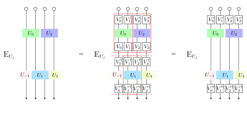
Figure 8 illustrates the fact that, at integer time $t$, the probability distribution of $W(t)$ is invariant under the transformation

$$W(t)\ \mapsto\ \left(\mbox{$\bigotimes_{x}$}V^{\prime}_{x}\right)^{\dagger}W(t)\left(\mbox{$\bigotimes_{x}$}V^{\prime}_{x}\right)\ ,$$ (108)

for any string of local Clifford unitaries $V^{\prime}_{1},\ldots,V^{\prime}_{L}\in\mathcal{C}_{N}$. This property translates to distribution (7) as

$$P_{t}\left([\mbox{$\bigoplus_{x}$}S_{x}^{-1}]{\bf u}^{\prime}\big{|}[\mbox{$\bigoplus_{x}$}S_{x}]{\bf u}\right)=P_{t}({\bf u}^{\prime}|{\bf u})$$ (109)

for any list of local symplectic matrices $S_{1},\ldots,S_{L}$. In order to prove Theorem 21 we exploit the fact that, at half-integer time $t$, the evolution operator displays a higher degree of symmetry. The probability distribution of $W(t)$ is invariant under the transformation

$$W(t)\ \mapsto\ \left(\mbox{$\bigotimes_{x}$}V_{x}\right)W(t)\left(\mbox{$\bigotimes_{x}$}V^{\prime}_{x}\right)\ ,$$ (110)

for any string of local Clifford unitaries $V_{1},V^{\prime}_{1},\ldots,V_{L},V^{\prime}_{L}\in\mathcal{C}_{N}$. This translates onto $P_{t}({\bf u}^{\prime}|{\bf u})$ in a way analogous to (109).

Figure 8: Twirling technique. This figure illustrates the fact that the probability distribution of the evolution operator is invariant under local transformations. On the left we have a section of the circuit of Figure 1. On the middle we use the fact that, for any pair of local Clifford unitaries $V_{x},V_{x+1}$, the random two-site Clifford unitary $(V_{x}\otimes V_{x+1})U_{x}(V^{\prime}_{x}\otimes V^{\prime}_{x+1})$ has the same probability distribution than $U_{x}$. On the right we see that all local unitaries get cancelled except for those of the initial and final times. Note that if the time $t$ is integer or half-integer the invariance property of $W(t)$ is different according to equations (108) and (110).

In this section, we will present what is referred to as the twirling technique in the work Sünderhauf et al. (2018) and discuss how it applies to the random Clifford circuit model we consider.

We recollect that the definition of the evolution operator after an integer time $t$ is:

$$W(t) \equiv\big{[}(U_{1}\otimes U_{3}\otimes\cdots\otimes U_{L-1})(U_{0}\otimes U_{2}\otimes\cdots\otimes U_{L-2})\big{]}^{t}$$

$$=(U_{\text{odd}}U_{\text{even}})^{t}=(U_{\text{chain}})^{t}\ ,$$

and after a half-integer time $t$ is:

$$W(t)\equiv U_{\text{even}}\,(U_{\text{chain}})^{t-1/2}\ .$$

Lemma 10.

Consider a set of $2L$ single-site Clifford unitaries $V_{x},V^{\prime}_{x}\in\mathcal{C}_{N}$, these unitaries are fixed. At integer time $t$, the random evolution operator $W(t)$, as defined above, has the same probability distribution as

$$\left(\bigotimes_{x=0}^{L-1}V_{x}^{\prime\dagger}\right)W(t)\left(\bigotimes_{x=0}^{L-1}V^{\prime}_{x}\right)\ .$$ (111)

Similarly, at half-integer time $t$ the evolution operator $W(t)$ has the same probability distribution as

$$\left(\bigotimes_{x=0}^{L-1}V_{x}\right)W(t)\left(\bigotimes_{x=0}^{L-1}V^{\prime}_{x}\right)\ .$$ (112)

Proof.

First, we note that any uniformly distributed two-site Clifford unitary $U_{x}\in\mathcal{C}_{2N}$ has the same probability distribution as the unitary $(V_{x}\otimes V_{x+1})U_{x}(V^{\prime}_{x}\otimes V^{\prime}_{x+1})$ for any arbitrary choice of $V_{x},V_{x+1},V^{\prime}_{x},V^{\prime}_{x+1}\in\mathcal{C}_{N}$; this is denoted as single-site Haar invariance. Hence, we introduce the primed notation for the random two-site Clifford unitary $U_{x}$

$$U^{\prime}_{x} \equiv(V_{x}\otimes V_{x+1})U_{x}(V^{\prime}_{x}\otimes V^{\prime}_{x+1})\text{ for even }x\in\mathbb{Z}_{L}\ ,$$ (113)

$$U^{\prime}_{x} \equiv(V^{\prime}_{x}\otimes V^{\prime}_{x+1})^{-1}U_{x}(V_{x}\otimes V_{x+1})^{-1}\text{for odd }x\in\mathbb{Z}_{L}\ ,$$ (114)

where $V_{x},V_{x+1},V^{\prime}_{x},V^{\prime}_{x+1}\in\mathcal{C}_{N}$ are any arbitrary choice of single-site Clifford unitary. Consequently, the primed version of the global dynamics for integer $t$ becomes

$$W^{\prime}(t)=\left(\bigotimes_{x=0}^{L-1}V_{x}^{\prime\dagger}\right)W(t)\left(\bigotimes_{x=0}^{L-1}V^{\prime}_{x}\right)\ ,$$ (115)

and for half-integer $t$

$$W^{\prime}(t)=\left(\bigotimes_{x=0}^{L-1}V_{x}\right)W(t)\left(\bigotimes_{x=0}^{L-1}V^{\prime}_{x}\right)\ .$$ (116)

The single-site Haar invariance of the probability distributions of the primed and not-primed evolution operators are identical, this proves the result. ∎

Next, we will define Pauli invariance and state when it applies to our model.

Definition 11.

An $n$-qubit random unitary $U\in$ SU($2^{n}$) with probability distribution $P(U)$ is Pauli invariant if $P(U\sigma)=P(U)$ for all $\sigma\in\mathcal{P}_{n}$ and $U\in$ SU($2^{n}$).

Lemma 12.

At half-integer time $t$, the random evolution operator $W(t)$ is Pauli invariant.

Proof.

The proof of this lemma follows from lemma 10. When t is half-integer, $W(t)$ and $(\mbox{$\bigotimes_{x=0}^{L-1}$}V_{x})W(t)(\mbox{$\bigotimes_{x=0}^{L-1}$}V^{\prime}_{x})$ have identical probability distributions, where $V_{x},V^{\prime}_{x}\in\mathcal{C}_{n}$. Since $\mathcal{P}_{n}\subset\mathcal{C}_{n}$, we can choose $(\mbox{$\bigotimes_{x=0}^{L-1}$}V_{x})$ to be any element of the Pauli group. Hence, $W(t)$ is Pauli invariant. ∎

V.2 Half-integer times

Lemma 13.

At half-integer $t\geq t_{\text{scr}}$ the probability distribution of the evolved vector ${\bf u}^{t}=S(t){\bf u}^{0}$ conditioned on it being non-zero at every site is uniform:

$${\rm prob}\{{\bf u}^{t}={\bf v}|{\bf u}_{x}^{t}\neq{\bf 0},\forall x\in\mathbb{Z}_{L}\}=\frac{1}{(2^{2N}-1)^{L}}\ ,$$ (117)

for all vectors ${\bf v}$ that are non-zero at every site ${\bf v}_{x}\neq{\bf 0},\forall x\in\mathbb{Z}_{L}$.

Proof.

The proof of this lemma follows from the twirling technique discussed in Section V.1 lemma 10. The probability distribution of the evolved vector ${\bf u}^{t}=S(t){\bf u}^{0}$ is identical to

$${\bf u}^{t}=\left(\mbox{$\bigoplus_{x=0}^{L-1}$}X_{x}\right)S(t)\left(\mbox{$\bigoplus_{x=0}^{L-1}$}Y_{x}\right){\bf u}^{0},$$

where $X_{x},Y_{x}\in\mathcal{S}_{N}$ are arbitrary single-site matrices. Hence, since the choice of each $X_{x}$ is arbitrary, each $X_{x}$ is independent and uniformly distributed over all single-site symplectic matrices. Therefore, imposing the condition that the evolved vector is non-zero on every site, then, since the twirling matrices $X_{x}$ are independent and uniform, the probability distribution of the evolved vector at each site is independent and uniformly distributed over all non-zero vectors. The application of lemma 3 eventually provides the conditional probability (117). ∎

Theorem 14.

Let $\sigma_{{\bf u}^{\prime}}=\lambda W(t)\sigma_{\bf u}W(t)^{\dagger}$ be the evolution of any initial Pauli operator $\sigma_{\bf u}\neq\mathbbm{1}$. At any half-integer time $t$ larger than the scrambling time, in the interval $t\in[t_{\rm scr},2t_{\rm scr}]$ the probability distribution (7) for the evolved operator $\sigma_{{\bf u}^{\prime}}$ is close to uniform, namely

$$\sum_{{\bf u}^{\prime}}\left|P_{t}({\bf u}^{\prime}|{\bf u})-Q_{t}({\bf u}^{\prime})\right|\ \leq\ 33\times t\,L\,2^{-N}\ .$$ (118)

Remark. The following is an equivalent statement to Theorem 14 formulated in phase space, we then present a proof.

Theorem 14 (Alternative form). For any initial non-zero vector ${\bf u}^{0}\in\mathcal{V}_{\rm chain}$, the probability distribution of the time evolved vector ${\bf u}^{t}=S(t){\bf u}^{0}$, at any half-integer time in the interval $t\in[t_{\text{scr}},2t_{\text{scr}}]$, is approximately uniformly distributed over all non-zero vectors of the total system, and bounded by

$$\sum_{{\bf v}}\left|{\rm prob}\{{\bf u}^{t}={\bf v}\}-\frac{1}{2^{2NL}-1}\right|\leq 32\,tL2^{-N}+L2^{-2N}\ .$$

Proof.

Below we make use of:

$$\textrm{prob}(A) =\textrm{prob}(A\wedge B)+\textrm{prob}(A\wedge\bar{B})$$

$$=\textrm{prob}(A|B)\textrm{prob}(B)+\textrm{prob}(A|\bar{B})\textrm{prob}(\bar{B})$$

where $A$ and $B$ are events in a probability space.

Defining $q\equiv{\rm prob}\{{\bf u}^{t}_{x}\neq{\bf 0},\forall x\in\mathbb{Z}_{L}\}$, we rewrite ${\rm prob}\{{\bf u}^{t}={\bf v}\}$ as follows

$${\rm prob}\{{\bf u}^{t}={\bf v}\} =q\,{\rm prob}\{{\bf u}^{t}={\bf v}|{\bf u}^{t}_{x}\neq{\bf 0},\forall x\in\mathbb{Z}_{L}\}$$

$$+(1-q)({\rm prob}\{{\bf u}^{t}={\bf v}|\exists y\in\mathbb{Z}_{L}:{\bf u}^{t}_{y}={\bf 0}\}).$$

Adding and subtracting $q\frac{1}{2^{2NL}-1}$ in the sum and then applying the triangular inequality, we find that:

$$\sum_{{\bf v}}\left|{\rm prob}\{{\bf u}^{t}={\bf v}\}-\frac{1}{2^{2NL}-1}\right| \leq\sum_{{\bf v}}\left|q\,{\rm prob}\{{\bf u}^{t}={\bf v}|{\bf u}^{t}_{x}\neq{\bf 0}\,\forall x\}-\frac{1}{2^{2NL}-1}\right|$$

$$+(1-q)\sum_{{\bf v}}\left|{\rm prob}\{{\bf u}^{t}={\bf v}|\exists y\in\mathbb{Z}_{L}:{\bf u}^{t}_{y}={\bf 0}\}-\frac{1}{2^{2NL}-1}\right|\ .$$

We can upper bound the first term with $q\leq 1$ and apply lemma 13 to find that

$$q\sum_{{\bf v}}\left|{\rm prob}\{{\bf u}^{t}={\bf v}|{\bf u}^{t}_{x}\neq{\bf 0}\,\forall x\}-\frac{1}{2^{2NL}-1}\right|\leq L2^{-2N}\ .$$

To bound the second term we notice that the maximum value of the sum is 2, in fact:

$$(1-q)\sum_{{\bf v}}\left|{\rm prob}\{{\bf u}^{t}={\bf v}|\exists y\in\mathbb{Z}_{L}:{\bf u}^{t}_{y}={\bf 0}\}-\frac{1}{2^{2NL}-1}\right|$$

$$\leq(1-q)\sum_{{\bf v}}\left({\rm prob}\{{\bf u}^{t}={\bf v}|\exists y\in\mathbb{Z}_{L}:{\bf u}^{t}_{y}={\bf 0}\}+\frac{1}{2^{2NL}-1}\right)=2(1-q)$$

and use the result of lemma 9 to find that

$$(1-q)\leq 16tL2^{-N}\ .$$ (119)

This gives the stated result. ∎

V.3 Integer times

In this section, we will consider only initial vectors which are supported (i.e. non-zero) on a single site, ${\bf u}^{0}\in\mathcal{V}_{0}\subseteq\mathcal{V}_{\rm chain},$ and their time evolution at integer times only. The validity of the following lemma isn’t restricted to integer times or even quantum circuits.

Lemma 15.

Let ${\bf u}$ be a fixed non-zero element of $\mathbb{Z}_{2}^{2N}$. Let the probability distribution $P({\bf v})$ over ${\bf v}\in\mathbb{Z}_{2}^{2N}$ have the property that $P(S{\bf v})=P({\bf v})$ for any $S\in\mathcal{S}_{N}$ such that $S{\bf u}={\bf u}$. Then it must be of the form

$$P({\bf v})=\left\{\begin{array}[]{ll}q_{1}&\mbox{ if ${\bf v}={\bf 0}$}\\ q_{2}&\mbox{ if ${\bf v}={\bf u}$}\\ q_{3}&\mbox{ if $\langle{\bf v},{\bf u}\rangle=0$ and ${\bf v}\neq{\bf 0},{\bf u}$}\\ q_{4}&\mbox{ if $\langle{\bf v},{\bf u}\rangle=1$}\end{array}\right.\ ,$$ (120)

where the positive numbers $q_{i}$ are constrained by the normalization of $P({\bf v})$.

Proof.

We initially consider that ${\bf u}=(1,0,\ldots,0)^{T}$, and the subgroup of $\mathcal{S}_{N}$ that leaves ${\bf u}$ unchanged. If ${\bf v}={\bf 0}\text{ or }{\bf u}$, then the action of this subgroup has no effect, and hence we require a parameter for each in the distribution, $q_{1}$ and $q_{2}$ respectively. This is not the case for all other choices of ${\bf v}$, since the action of the subgroup will transform ${\bf v}$ into some other vector in $\mathbb{Z}_{2}^{2N}$. This transformation is constrained by the symplectic form:

$$\langle{\bf v},{\bf u}\rangle=\langle S{\bf v},S{\bf u}\rangle=\langle S{\bf v},{\bf u}\rangle\ ,$$ (121)

and hence the subgroup is composed of two subgroups, which transform ${\bf v}$ into another vector in $\mathbb{Z}_{2}^{2N}$ that has the same value for the symplectic form. Furthermore, the two subgroups are such they can map any vector to any other vector with the same value for the symplectic form.

This can be seen by considering the case where ${\bf v}=(0,1,\ldots,0)^{T}$, so $\langle{\bf u},{\bf v}\rangle=1$. The subgroup that keeps ${\bf u}=(1,0,...,0)^{T}$ unchanged consists of all the elements of $\mathcal{S}_{N}$ with ${\bf u}$ as the first column of the matrix. Hence, by lemma 1, we can select the second column of the matrix to be any vector which has symplectic form of 1 with the first column, which is ${\bf u}$. Thus, we can map ${\bf v}$ to any other vector with symplectic form one with ${\bf u}$, which is also unchanged. Then, by noting that the product of symplectic matrices is a symplectic matrix, the subgroup can map any vector with symplectic form of one with ${\bf u}$ to any other. Similarly, this argument applies to the other case where the symplectic form has a value of zero.

Then since $P(S{\bf v})=P({\bf v})$, all vectors that give the same value for $\langle{\bf v},{\bf u}\rangle$ have the same probability. Thus, we get the probability distribution in (120).

Finally, we note that since via a symplectic transformation ${\bf u}$ can be mapped to any other vector in $\mathbb{Z}_{2}^{2N}$, and that the product of two symplectic matrices is symplectic, this result applies for any ${\bf u}\in\mathbb{Z}_{2}^{2N}$. ∎

Lemma 16.

For an initial vector ${\bf u}^{0}\in\mathcal{V}_{0}$ supported on location $x=0$, the probability that the value of the symplectic form between the evolved vector ${\bf u}^{t}=S_{\text{chain}}^{t}{\bf u}^{0}$, with integer $t$, and the initial vector, $\langle{\bf u}^{t},{\bf u}^{0}\rangle=\langle{\bf u}_{0}^{t},{\bf u}_{0}^{0}\rangle$ is equal to $s$, has an $s$-independent upper bound given by:

$${\rm prob}\{\langle{\bf u}_{0}^{t},{\bf u}_{0}^{0}\rangle=s\}\leq\frac{1}{2}+8\,t\,2^{-N}.$$ (122)

Furthermore, this result is independent from the location of the support of ${\bf u}^{0}$ provided that it is a single site.

Proof.

To prove this lemma we proceed similarly as in Lemma 9. That is, we consider a sequence of gates in the causal past of ${\bf u}_{0}^{t}$ with an elbow shape (see example in Figure 7). More concretely, we write ${\bf u}_{0}^{t}$ as

$${\bf u}_{1-t}^{t/2} =B_{1-t}\cdots B_{-2}B_{-1}A_{0}{\bf u}_{0}^{0}\ ,$$ (123)

$${\bf u}_{1-t}^{t/2+1/2} =D_{-t}{\bf u}_{1-t}^{t/2}\ ,$$ (124)

$${\bf u}_{0}^{t} =C_{-1}\cdots C_{2-t}C_{1-t}{\bf u}_{1-t}^{t/2+1/2}+{\bf w}\ ,$$ (125)

where, crucially, the random vector ${\bf w}$ is independent of the random matrix $D_{-t}$. This vector ${\bf w}$ is defined in a way similar to (96).

Next, we follow a sequence of steps similar to those from (105) to (107). First we write

$${\rm prob}\!\left\{\langle{\bf u}_{0}^{0},{\bf u}_{0}^{t}\rangle=s\right\}$$

$$=\ {\rm prob}\!\left\{\langle{\bf u}_{0}^{0},{\bf u}_{0}^{t}\rangle=s\mbox{ and }{\bf u}_{1-t}^{t/2}={\bf 0}\right\}+{\rm prob}\!\left\{\langle{\bf u}_{0}^{0},{\bf u}_{0}^{t}\rangle=s\mbox{ and }{\bf u}_{1-t}^{t/2}\neq{\bf 0}\right\}$$

$$\leq\ {\rm prob}\!\left\{{\bf u}_{1-t}^{t/2}={\bf 0}\right\}+{\rm prob}\!\left\{\langle{\bf u}_{0}^{0},{\bf u}_{0}^{t}\rangle=s\mbox{ and }{\bf u}_{1-t}^{t/2}\neq{\bf 0}\right\}\ .$$ (126)

Second, we bound the first term by using the recursive relation (89) as

$${\rm prob}\!\left\{{\bf u}_{1-t}^{t/2}={\bf 0}\right\}\leq 2\,t\,2^{-2N}\ .$$ (127)

Third, we introduce the uniformly distributed random vectors ${\bf u},{\bf u}^{\prime}\in\mathbb{Z}_{2}^{2N}$, which are independent of the gates $S_{1-t},S_{2-t},\ldots,S_{-2}$, and write

$${\rm prob}\!\left\{\langle{\bf u}_{0}^{0},{\bf u}_{0}^{t}\rangle=s\mbox{ and }{\bf u}_{1-t}^{t/2}\neq{\bf 0}\right\}$$

$$=\ {\rm prob}\!\left\{{\bf u}_{0}^{0\,T}JC_{-1}\cdots C_{1-t}{\bf u}_{1-t}^{t/2+1/2}=s+\langle{\bf u}_{0}^{0},{\bf w}\rangle\mbox{ and }{\bf u}_{1-t}^{t/2}\neq{\bf 0}\right\}$$

$$\leq\ {\rm d}\!\left({\bf u}_{1-t}^{t/2+1/2},{\bf u}\right)+{\rm prob}\!\left\{{\bf u}_{0}^{0\,T}JC_{-1}\cdots C_{1-t}{\bf u}=s+\langle{\bf u}_{0}^{0},{\bf w}\rangle\mbox{ and }{\bf u}_{1-t}^{t/2}\neq{\bf 0}\right\}$$

$$\leq\ {\rm d}\!\left({\bf u}_{1-t}^{t/2+1/2},{\bf u}\right)+{\rm prob}\!\left\{{\bf u}_{0}^{0\,T}JC_{-1}\cdots C_{1-t}{\bf u}=s+\langle{\bf u}_{0}^{0},{\bf w}\rangle\right\}$$

$$\leq\ {\rm d}\!\left({\bf u}_{1-t}^{t/2+1/2},{\bf u}\right)+{\rm d}\!\left(JC_{-1}^{T}J{\bf u}_{0}^{0},{\bf u}^{\prime}\right)+{\rm prob}\!\left\{{\bf u}^{\prime T}JC_{-2}\cdots C_{1-t}{\bf u}=s+\langle{\bf u}_{0}^{0},{\bf w}\rangle\right\}\ .$$ (128)

Fourth, using (106) we can write the bounds

$${\rm d}\!\left({\bf u}_{1-t}^{t/2+1/2},{\bf u}\right)\leq\ 2^{1-4N}\ ,$$

$${\rm d}\!\left(JC_{-1}^{T}J{\bf u}_{0}^{0},{\bf u}^{\prime}\right)\leq\ 2^{1-4N}\ .$$ (129)

Fifth, in order to bound the third term in (128) we note that, for any non-zero ${\bf a}\in\mathbb{Z}_{2}^{2N}$ we have ${\rm prob}\{{\bf u}^{\prime T}{\bf a}=s\}=1/2$, for both $s=0,1$, therefore

$${\rm prob}\!\left\{{\bf u}^{\prime T}JC_{-2}\cdots C_{1-t}{\bf u}=s+\langle{\bf u}_{0}^{0},{\bf w}\rangle\right\}$$

$$=\ {\rm prob}\!\left\{{\bf u}^{\prime T}JC_{-2}\cdots C_{1-t}{\bf u}=s+\langle{\bf u}_{0}^{0},{\bf w}\rangle\mbox{ and }C_{-2}\cdots C_{1-t}{\bf u}\neq{\bf 0}\right\}$$

$$+\ {\rm prob}\!\left\{{\bf u}^{\prime T}JC_{-2}\cdots C_{1-t}{\bf u}=s+\langle{\bf u}_{0}^{0},{\bf w}\rangle\mbox{ and }C_{-2}\cdots C_{1-t}{\bf u}={\bf 0}\right\}\ .$$

Next we bound the first term by using the fact that the uniformly distributed vector ${\bf u}^{\prime}$ is independent of ${\bf a}:=JC_{-2}\cdots C_{1-t}{\bf u}$ and $\langle{\bf u}_{0}^{0},{\bf w}\rangle$, as

$${\rm prob}\!\left\{{\bf u}^{\prime T}{\bf a}=s+\langle{\bf u}_{0}^{0},{\bf w}\rangle\mbox{ and }{\bf a}\neq{\bf 0}\right\}\leq{\rm prob}\!\left\{{\bf u}^{\prime T}{\bf a}=s+\langle{\bf u}_{0}^{0},{\bf w}\rangle\big{|}\,{\bf a}\neq{\bf 0}\right\}=\frac{1}{2}\ .$$

The second term can be easily bounded as

$${\rm prob}\!\left\{{\bf u}^{\prime T}JC_{-2}\cdots C_{1-t}{\bf u}=s+\langle{\bf u}_{0}^{0},{\bf w}\rangle\mbox{ and }C_{-2}\cdots C_{1-t}{\bf u}={\bf 0}\right\}$$

$$\leq\ {\rm prob}\!\left\{C_{-2}\cdots C_{1-t}{\bf u}={\bf 0}\right\}\ \leq\ 8(t-2)2^{-N}\ ,$$

where the last inequality follows from Lemma 6. Combining the above two bounds we obtain

$${\rm prob}\!\left\{{\bf u}^{\prime T}JC_{-2}\cdots C_{1-t}{\bf u}=s+\langle{\bf u}_{0}^{0},{\bf w}\rangle\right\}\ \leq\ \frac{1}{2}+8(t-2)2^{-N}\ .$$

Sixth, putting everything together back from (126) we arrive at

$${\rm prob}\!\left\{\langle{\bf u}_{0}^{0},{\bf u}_{0}^{t}\rangle=s\right\}\leq\ 2\,t\,2^{-2N}+4\,2^{-4N}+\frac{1}{2}+8(t-2)2^{-N}$$

$$\leq\ \frac{1}{2}+8\,t\,2^{-N},$$

as we wanted to show. ∎

Lemma 17.

For an initial vector ${\bf u}^{0}\in\mathcal{V}_{0}$ supported at $x=0$, the probability distribution of the evolved vector ${\bf u}^{t}=S_{\text{chain}}^{t}{\bf u}^{0}$ at integer times, conditioned on the evolved vector being non-zero at every site and different from the initial single-site non-zero vector, ${\bf u}_{x}^{t}\neq 0\ \forall x\in\mathbb{Z}_{L}\text{ and }{\bf u}_{0}^{t}\neq{\bf u}_{0}^{0}$, after the scrambling time $t_{\text{scr}}$ is of the form

$${\rm prob}\{{\bf u}^{t}|{\bf u}_{x}^{t}\neq 0\ \forall x\in\mathbb{Z}_{L},{\bf u}_{0}^{t}\neq{\bf u}_{0}^{0}\}\leq\frac{1}{(2^{2N}-1)^{L-1}}\left\{\begin{array}[]{cc}\frac{8t2^{-N}+1/2}{2^{2N-1}-2}&\text{ if }\langle{\bf u}_{0}^{t},{\bf u}_{0}^{0}\rangle=0\\ \frac{8t2^{-N}+1/2}{2^{2N-1}}&\text{ if }\langle{\bf u}_{0}^{t},{\bf u}_{0}^{0}\rangle=1\end{array}\right.\ ,$$

and before the scrambling time for all sites within the causal light-cone the probability distribution is of the form

$${\rm prob}\{{\bf u}^{t}|{\bf u}_{x}^{t}\neq 0\ \forall x\in[-2t+1,2t],{\bf u}_{0}^{t}\neq{\bf u}_{0}^{0}\}$$

$$\hskip 56.9055pt\leq\frac{1}{(2^{2N}-1)^{4t-1}}\left\{\begin{array}[]{cc}\frac{8t2^{-N}+1/2}{2^{2N-1}-2}&\text{ if }\langle{\bf u}_{0}^{t},{\bf u}_{0}^{0}\rangle=0\\ \frac{8t2^{-N}+1/2}{2^{2N-1}}&\text{ if }\langle{\bf u}_{0}^{t},{\bf u}_{0}^{0}\rangle=1\end{array}\right.\ .$$ (132)

Furthermore, this result holds for any choice of the single-site at which the initial vector is non-zero.

Proof.

The proof of this lemma uses the twirling technique discussed in Section V.1 lemma 10. The probability distribution of the evolved vector ${\bf u}^{t}=(S_{\text{chain}})^{t}{\bf u}^{0}$ at integer times is identical to

$${\bf u}^{t} =\left(\mbox{$\bigoplus_{x=0}^{L-1}$}X_{x}\right)S_{\text{chain}}^{t}\left(\mbox{$\bigoplus_{x=0}^{L-1}$}X_{x}^{-1}\right){\bf u}^{0}$$

$$=\left(\mbox{$\bigoplus_{x=0}^{L-1}$}X_{x}\right)S_{\text{chain}}^{t}\left(X_{0}^{-1}{\bf u}_{0}^{0}\,\mbox{$\bigoplus_{x=1}^{L-1}$}{\bf 0}\right)$$ (133)

where $X_{x}\in\mathcal{S}_{N}$ are arbitrary single-site symplectic matrices. Equation (133) follows from the fact that ${\bf u}^{0}$ has been assumed supported at $x=0$, therefore $\left(\mbox{$\bigoplus_{x=0}^{L-1}$}X_{x}^{-1}\right){\bf u}^{0}$ is supported at $x=0$ as well. If we restrict $X_{0}$ to the elements of $\mathcal{S}_{N}$ that satisfy $X_{0}{\bf u}_{0}^{0}={\bf u}_{0}^{0}$, then the probability distribution of ${\bf u}^{t}$ is identical to $\left(\bigoplus_{x=0}^{L-1}X_{x}\right){\bf u}^{t}$. Since the choice of symplectic matrices $\bigoplus_{x=0}^{L-1}X_{x}$ to twirl is arbitrary, we can take each single-site matrix to be independent and uniformly distributed over all single-site symplectic matrices, except for $X_{0}$ which is uniformly distributed over the restricted set satisfying $X_{0}{\bf u}_{0}^{0}={\bf u}_{0}^{0}$. Then, we condition on the evolved vector being non-zero at all sites $x$ and different for the initial single-site non-zero vector, ${\bf u}_{x}^{t}\neq 0\ \forall x\in\mathbb{Z}_{L}\text{ and }{\bf u}_{0}^{t}\neq{\bf u}_{0}^{0}$. Therefore under this condition, the evolved vector at each site is independent and uniformly distributed over all non-zero vectors (lemma 3) apart from the initial vector ${\bf u}_{0}^{0}$. On the vector space $\mathcal{V}_{0}$ we invoke lemma 15, and hence the evolved vector ${\bf u}_{0}^{t}$ ($\neq{\bf 0},{\bf u}_{0}^{0}$) at $x=0$ is uniformly distributed over all the vectors with the same symplectic form with ${\bf u}_{0}^{0}$, $\langle{\bf u}_{0}^{t},{\bf u}_{0}^{0}\rangle$. Hence, using lemma 16, which gives an upper bound for the probability of $\langle{\bf u}_{0}^{t},{\bf u}_{0}^{0}\rangle\in\{0,1\}$, we get the stated result. ∎

The following theorem establishes approximate Pauli mixing: the probability that ${\bf u}$ evolves onto ${\bf u}^{\prime}$ after a time $t$ given by:

$$P_{t}({\bf u}^{\prime}|{\bf u})=\mathop{\mathbb{E}}_{\{U_{x}\}}\left|2^{-NL}\tr(\sigma_{{\bf u}^{\prime}}W(t)\sigma_{{\bf u}}W(t)^{\dagger})\right|\ ,$$ (134)

is close to the uniform distribution over all non-zero vectors ${\bf u}^{\prime}$ in the causal subspace (8) denoted by $Q_{t}({\bf u}^{\prime})$. After the scrambling time $t\geq t_{\rm scr}$, $Q_{t}({\bf u}^{\prime})$ is the uniform distribution over all non-zero vectors in the total phase space $\mathcal{V}_{\rm chain}$.

Theorem 18.

(Approximate Pauli mixing) If the initial Pauli operator $\sigma_{\bf u}$ is supported at site $x=0$ then the probability distribution (7) for its evolution $\sigma_{{\bf u}^{\prime}}$ is close to uniform inside the light cone

$$\sum_{{\bf u}^{\prime}}\left|P_{t}({\bf u}^{\prime}|{\bf u})-Q_{t}({\bf u}^{\prime})\right|\ \leq\ 130\times t^{2}\,2^{-N}\ ,$$ (135)

for any integer or half-integer time $t\in[1/2,2t_{\rm scr}]$. An analogous statement holds for any other initial location $x\neq 0$.

Remark. The following is an alternative enunciation of Theorem 18 formulated in phase space rather than Hilbert space. A proof of this alternative form then follows.

Theorem 18 (Alternative form). For an initial vector supported at $x=0$, the evolved vector ${\bf u}^{t}=S_{\text{chain}}^{t}{\bf u}^{0}$, at integer times, is approximately uniformly distributed over all non-zero vectors within the light-cone. For any $t\in[1,t_{\rm scr}]$ and $x\in[-2t+1,2t]$ we have:

$$\sum_{{\bf v}\in\mathbb{Z}_{2}^{8Nt}}\left|{\rm prob}\{{\bf u}^{t}={\bf v}\}-\frac{1}{2^{8Nt}-1}\right|\leq\ 32t(4t+1)2^{-N}+4t2^{-2N}$$ (136)

For any $t\in[t_{\rm scr},2t_{\rm scr}]$ it holds:

$$\sum_{{\bf v}\in\mathbb{Z}_{2}^{2NL}}\left|{\rm prob}\{{\bf u}^{t}={\bf v}\}-\frac{1}{2^{2NL}-1}\right|\leq 32t(L+1)2^{-N}+L2^{-2N}$$

Proof.

Let us consider the case $t\geq t_{\rm scr}$ first. Similarly to the proof of Theorem 14 we employ

$$\textrm{prob}(A) =\textrm{prob}(A\wedge B)+\textrm{prob}(A\wedge\bar{B})$$

$$=\textrm{prob}(A|B)\textrm{prob}(B)+\textrm{prob}(A|\bar{B})\textrm{prob}(\bar{B})$$

where $A$ and $B$ are events in a probability space. With $q\equiv{\rm prob}\{{\bf u}^{t}_{x}\neq{\bf 0}\,\forall x\in\mathbb{Z}_{L}\wedge{\bf u}_{0}^{t}\neq{\bf u}_{0}^{0}\}$, ${\rm prob}\{{\bf u}^{t}={\bf v}\}$ is then rewritten in the following way

$${\rm prob}\{{\bf u}^{t}={\bf v}\} =q\,{\rm prob}\{{\bf u}^{t}={\bf v}|{\bf u}^{t}_{x}\neq{\bf 0}\,\forall x\in\mathbb{Z}_{L}\wedge{\bf u}_{0}^{t}\neq{\bf u}_{0}^{0}\}$$

$$+(1-q)({\rm prob}\{{\bf u}^{t}={\bf v}|\,\exists x\in\mathbb{Z}_{L}\,\textrm{such that}\,{\bf u}^{t}_{x}={\bf 0}\vee{\bf u}_{0}^{t}={\bf u}_{0}^{0}\})\ ,$$

Summing and subtracting $q\frac{1}{2^{2NL}-1}$ into the sum over ${\bf v}$ and using the triangular inequality we find that

$$\sum_{{\bf v}}\left|{\rm prob}\{{\bf u}^{t}={\bf v}\}-\frac{1}{2^{2NL}-1}\right|$$

$$\leq q\sum_{{\bf v}}\left|{\rm prob}\{{\bf u}^{t}={\bf v}|{\bf u}^{t}_{x}\neq{\bf 0}\,\forall x\in\mathbb{Z}_{L},{\bf u}_{0}^{t}\neq{\bf u}_{0}^{0}\}-\frac{1}{2^{2NL}-1}\right|$$

$$+(1-q)\sum_{{\bf v}}\left|{\rm prob}\{{\bf u}^{t}={\bf v}|\,\exists x\in\mathbb{Z}_{L}\,\textrm{such that}\,{\bf u}^{t}_{x}={\bf 0}\vee{\bf u}_{0}^{t}={\bf u}_{0}^{0}\}-\frac{1}{2^{2NL}-1}\right|\ .$$

We can bound the first term using $q\leq 1$ and apply lemma 17 to find that

$$q\sum_{{\bf v}}\left|{\rm prob}\{{\bf u}^{t}={\bf v}|{\bf u}^{t}_{x}\neq{\bf 0}\,\forall x\in\mathbb{Z}_{L},{\bf u}_{0}^{t}\neq{\bf u}_{0}^{0}\}-\frac{1}{2^{2NL}-1}\right|\leq 16t2^{-N}+(L+1)2^{-2N}\ .$$

To evaluate the second term above, we upper bound the sum with its maximum value of 2 and use the result of lemma 9 to find that

$$(1-q)\sum_{{\bf v}}\left|{\rm prob}\{{\bf u}^{t}={\bf v}|\,\exists x\in\mathbb{Z}_{L}\,\textrm{such that}\,{\bf u}^{t}_{x}={\bf 0}\vee{\bf u}_{0}^{t}={\bf u}_{0}^{0}\}-\frac{1}{2^{2NL}-1}\right|\leq 32t(L+1)2^{-N}\ .$$

Combining, this gives the stated result for integer times after the scrambling time.

To derive the results for integer times before the scrambling time, we note that the derivation is identical with the substitution $L\rightarrow 4t$, which agree when $t=t_{\text{scr}}$ (and after this time). ∎

V.4 Approximate mixing with arbitrary initial state

Consider a subsystem of the chain comprising $L_{\mathrm{s}}$ consecutive sites, where $L_{\mathrm{s}}$ is even. Without loss of generality we choose this subsystem to be $\{1,2,\ldots,L_{\mathrm{s}}\}\subseteq\mathbb{Z}_{L}$. We analyse the state of this subsystem at times

$$t\leq\frac{L-L_{\mathrm{s}}}{4}\ .$$ (137)

This condition ensures that the left backwards wave front of ${\bf u}_{1}^{t}$ and the right backwards wave front of ${\bf u}_{L_{\mathrm{s}}}^{t}$ do not collide. Without this condition, the analysis becomes very complicated.

Lemma 19.

Consider an initial vector ${\bf u}^{0}\in\mathcal{V}_{\rm chain}$ supported on all lattice sites (${\bf u}_{x}^{0}\neq{\bf 0}$ for all $x\in\mathbb{Z}_{L}$), and its evolution at time $t$, ${\bf u}^{t}$. Define the random variable $s_{x}=\langle\mathbf{{\bf u}}^{t}_{x},{\bf u}^{0}_{x}\rangle$ at each site of the region $x\in\{1,\ldots,L_{\mathrm{s}}\}\subseteq\mathbb{Z}_{L}$, where $L_{\mathrm{s}}$ is even. Then we have

$$P(s_{1},\ldots,s_{L_{\mathrm{s}}}) \leq 2^{-L_{s}}+32\,t\,3^{\frac{L_{s}}{2}+1}\,2^{-N}\ ,$$ (138)

as long as $t\leq(L-L_{\mathrm{s}})/4$.

Proof.

The value of the random vectors ${\bf u}^{t}_{1},\ldots,{\bf u}^{t}_{L_{\mathrm{s}}}$ is only determined by the random matrices $S_{2-2t},\ldots,S_{L_{\mathrm{s}}+2t-2}$. The rest of matrices $S_{x}$ are not contained in the causal past of the region under consideration $\{1,2,\ldots,L_{\mathrm{s}}\}$. In order to simplify this proof, we will replace $S_{2-2t},\ldots,S_{L_{\mathrm{s}}+2t-2}$ by a new set of random variables defined in what follows.

Let us label by $y\in\{1,\ldots,L_{\mathrm{s}}/2\}$ the pair of neighbouring sites $\{2y-1,2y\}\subseteq\{1,\ldots,L_{\mathrm{s}}\}$. For each pair $y$ we consider a given non-zero vector $\mathbf{a}_{y}\in\mathbb{Z}_{2}^{4N}$ and define the random variables

$$\mathbf{b}_{y} =S_{2y-1}^{-1}\mathbf{a}_{y}\ ,$$ (139)

$$h_{y} =\left\langle\mathbf{a}_{y},{\bf u}^{t}_{2y-1}\oplus{\bf u}^{t}_{2y}\right\rangle=\left\langle\mathbf{b}_{y},{\bf u}^{t-1/2}_{2y-1}\oplus{\bf u}^{t-1/2}_{2y}\right\rangle\ .$$ (140)

The left-most random contribution to $h_{y}$ is the matrix $S_{2y-2t}$, or equivalently the vector ${\bf w}_{y}$, defined through

$$\tilde{\bf w}_{y}\oplus{\bf w}_{y}=S_{2y-2t}({\bf u}^{0}_{2y-2t}\oplus{\bf u}^{0}_{2y-2t+1})\ .$$ (141)

We note that ${\bf w}_{y}\in\mathcal{V}_{2y-2t+1}$. This contribution and others are illustrated in Figure 9.

Figure 9: This figure represents the region $\{1,2,\ldots,6\}$ at time $t=2$, and its causal past back to $t=0$. (Hence $L_{\mathrm{s}}=6$.) All the random matrices $S_{-2},\ldots,S_{8}$ contribute to the value of the vectors ${\bf u}^{t}_{1},\ldots,{\bf u}^{t}_{6}$. The left-most contribution to the vector ${\bf u}^{t}_{1}$ is the matrix $S_{-2}$, or equivalently the vector ${\bf w}_{1}$. The given vector $\mathbf{a}_{y}$ associated to the pair of neighbouring sites $y$, and its 1/2-step backwards time translations $\mathbf{b}_{y}$, are also represented.

The contribution of the vector ${\bf w}_{y}$ to $h_{y}$ (and ${\bf u}^{t-1/2}_{2y-1}$) is “transmitted through” the matrices $S_{2y-2}$, $S_{2y-3}$, $\ldots$, $S_{2y-2t+2}$, $S_{2y-2t+1}$. More precisely, ${\bf w}_{y}$ is mapped via the matrix product

$$F_{y}=C_{2y-2}C_{2y-3}\cdots C_{2y-2t+2}C_{2y-2t+1}\ ,$$ (142)

where we have used decomposition (28). We denote by ${\bf v}_{y}$ all contributions to ${\bf u}^{t-1/2}_{2y-1}$ that are not $F_{y}{\bf w}_{y}$,

$${\bf v}_{y}=({\bf u}_{2y-1}^{t-1/2}+F_{y}{\bf w}_{y})\oplus{\bf u}_{2y}^{t-1/2}.$$ (143)

We remark that ${\bf v}_{y}\in\mathcal{V}_{2y-1}\oplus\mathcal{V}_{2y}$. The last random variable that we need to define is $g_{y}=\langle\mathbf{b}_{y},{\bf v}_{y}\rangle$, which together with (140) allows us to write

$$h_{y}=\left\langle\mathbf{b}_{y},F_{y}{\bf w}_{y}+{\bf v}_{y}\right\rangle=\left\langle\mathbf{b}_{y},F_{y}{\bf w}_{y}\right\rangle+g_{y}\ .$$ (144)

Note the slight abuse of notation in that we write $F_{y}{\bf w}_{y}$ instead of $F_{y}{\bf w}_{y}\oplus\mathbf{0}$.

In summary, we have replaced the variables $S_{2-2t},\ldots,S_{L_{\mathrm{s}}+2t-2}$ by the variables ${\bf w}_{y},\mathbf{b}_{y},F_{y},g_{y}$ for $y=1,\ldots,L_{\mathrm{s}}/2$. (We are not using ${\bf v}_{y},\tilde{\bf w}_{y}$ any more.) These variables are not all independent, but they satisfy the following independence relations:

• ${\bf w}_{1},\mathbf{b}_{1},\ldots,{\bf w}_{L_{\mathrm{s}}/2},\mathbf{b}_{L_{\mathrm{s}}/2}$ are independent and uniform.

• ${\bf w}_{y}$ is independent of $g_{y^{\prime}}$ for all $y^{\prime}\geq y$.

• $F_{y}$ is independent of ${\bf w}_{y^{\prime}}$ and $\mathbf{b}_{y^{\prime\prime}}$ for all $y^{\prime}\leq y$ and $y^{\prime\prime}\geq y$.

To continue with the proof it is convenient to introduce the following notation:

$${\bf u}_{\geq y} =({\bf u}_{y},{\bf u}_{y+1},\ldots,{\bf u}_{L_{\mathrm{s}}/2})\ ,$$ (145)

$${\bf u}_{\leq y} =({\bf u}_{1},{\bf u}_{2},\ldots,{\bf u}_{y})\ ,$$ (146)

and analogously for $>,<$ and the rest of variables $\mathbf{b}_{y},F_{y},g_{y}$. This allows us to write the joint probability distribution of $h_{1},\ldots,h_{L_{\mathrm{s}}/2}$ as

$$P(h_{\geq 1})=\sum_{{\bf w}_{\geq 1},\mathbf{b}_{\geq 1},F_{\geq 1},g_{\geq 1}}P({\bf w}_{\geq 1},\mathbf{b}_{\geq 1},F_{\geq 1},g_{\geq 1})\prod_{y}\delta\left(h_{y},\left\langle\mathbf{b}_{y},F_{y}{\bf w}_{y}\right\rangle+g_{y}\right)\ .$$ (147)

Equation (147) follows directly from the definition of the Kronecker-delta. Note that we can write the above distribution $P({\bf w}_{\geq 1},\mathbf{b}_{\geq 1},F_{\geq 1},g_{\geq 1})$ as

$$P(\mathbf{w}_{\geq 1},\mathbf{b}_{\geq 1},F_{\geq 1},g_{\geq 1})=\sum_{S_{0},S_{1},\ldots,S_{L-1}}P(S_{0})P(S_{1})\cdots P(S_{L-1})\times$$

$$\hskip 28.45274pt\times\prod_{y=1}^{L_{s}/2}\delta\!\left(\mathbf{w}_{y},S_{2y-2t}[\mathbf{u}^{0}_{2y-2t}\oplus\mathbf{u}^{0}_{2y-2t+1}]\right)\times\delta\!\left(\mathbf{b}_{y},S^{-1}_{2y-1}\mathbf{a}_{y}\right)\times$$

$$\hskip 28.45274pt\times\delta\!\left(F_{y},C_{2y-2}\cdots C_{2y-2t+1}\right)\times\delta\left(g_{y},\left\langle\mathbf{b}_{y},({\bf u}_{2y-1}^{t-1/2}+F_{y}{\bf w}_{y})\oplus{\bf u}_{2y}^{t-1/2}\right\rangle\right).$$ (148)

The following sum-rule is repeatedly exploited below, where ${\bf 0}_{2N}$ denotes the $2N\times 2N$ matrix with all entries equal to $0$, instead $\bf 0$ is the vector with $2N$ components equal to $0$.

$$\sum_{{\bf w}_{1}}P({\bf w}_{1})\delta\left(h_{1},\left\langle\mathbf{b}_{1},F_{1}{\bf w}_{1}\right\rangle+g_{1}\right)=\left\{\begin{array}[]{ll}\delta\left(h_{1},g_{1}\right)&\mbox{ if }(F_{1}\oplus{\bf 0}_{2N})^{T}J\mathbf{b}_{1}=\mathbf{0}\ ,\\ 1/2&\mbox{ otherwise.}\end{array}\right.$$ (149)

Equation (149) is obtained as follows. We first note that

$$\left\langle\mathbf{b}_{1},F_{1}{\bf w}_{1}\oplus{\bf 0}\right\rangle=\left\langle\mathbf{b}_{1},(F_{1}\oplus{\bf 0}_{2N})({\bf w}_{1}\oplus{\bf 0})\right\rangle=\mathbf{b}_{1}^{T}J(F_{1}\oplus{\bf 0}_{2N})({\bf w}_{1}\oplus{\bf 0})\ .$$

If $(F_{1}\oplus{\bf 0}_{2N})^{T}J\mathbf{b}_{1}=\mathbf{0}$, the first of equations (149) follows from the normalisation of the probability $P({\bf w}_{1})$. If $(F_{1}\oplus{\bf 0}_{2N})^{T}J\mathbf{b}_{1}\neq\mathbf{0}$, since the values of ${\bf w}_{1}$ are distributed uniformly over all the vectors of $\mathbb{Z}_{2}^{2N}$, implying that $P({\bf w}_{1})=\frac{1}{2^{2N}}$, then $\left\langle\mathbf{b}_{1},F_{1}{\bf w}_{1}\right\rangle$ takes half of the times the value $0$ and half of the times the value $1$. Recall that $F_{1}$ and $\mathbf{b}_{1}$ are fixed in (149). The second equation of (149) then follows.

Using $\delta(h,h^{\prime})\leq 1$ for all $h,h^{\prime}$ and (149) we can write

$$P(h_{\geq 1})=\sum_{{\bf w}_{\geq 1},\mathbf{b}_{\geq 1},F_{\geq 1},g_{\geq 1}}P({\bf w}_{1})P({\bf w}_{\geq 2},\mathbf{b}_{\geq 1},F_{\geq 1},g_{\geq 1})\prod_{y}\delta\left(h_{y},\left\langle\mathbf{b}_{y},F_{y}{\bf w}_{y}\right\rangle+g_{y}\right)$$

$$\leq\sum_{{\bf w}_{\geq 2},\mathbf{b}_{\geq 1},F_{\geq 1},g_{\geq 1}}\delta\left((F_{1}\oplus{\bf 0}_{2N})^{T}J\mathbf{b}_{1},\mathbf{0}\right)P({\bf w}_{\geq 2},\mathbf{b}_{\geq 1},F_{\geq 1},g_{\geq 1})\prod_{y\geq 2}\delta\left(h_{y},\left\langle\mathbf{b}_{y},F_{y}{\bf w}_{y}\right\rangle+g_{y}\right)+$$

$$+\frac{1}{2}\sum_{{\bf w}_{\geq 2},\mathbf{b}_{\geq 2},F_{\geq 2},g_{\geq 2}}P({\bf w}_{\geq 2},\mathbf{b}_{\geq 2},F_{\geq 2},g_{\geq 2})\prod_{y\geq 2}\delta\left(h_{y},\left\langle\mathbf{b}_{y},F_{y}{\bf w}_{y}\right\rangle+g_{y}\right)$$

$$\leq{\rm prob}\{(F_{1}\oplus{\bf 0}_{2N})^{T}J\mathbf{b}_{1}=\mathbf{0}\}+$$

$$+\frac{1}{2}\sum_{{\bf w}_{\geq 2},\mathbf{b}_{\geq 2},F_{\geq 2},g_{\geq 2}}P({\bf w}_{\geq 2},\mathbf{b}_{\geq 2},F_{\geq 2},g_{\geq 2})\prod_{y\geq 2}\delta\left(h_{y},\left\langle\mathbf{b}_{y},F_{y}{\bf w}_{y}\right\rangle+g_{y}\right)$$

To bound the term associated with the case $(F_{1}\oplus{\bf 0}_{2N})^{T}J\mathbf{b}_{1}\neq\mathbf{0}$ we extended the sum over $\mathbf{b}_{1},F_{1}$ from the values satisfying $(F_{1}\oplus{\bf 0}_{2N})^{T}J\mathbf{b}_{1}\neq\mathbf{0}$ to all values. Since the variables $\mathbf{b}_{1},F_{1},g_{1}$ do not appear in any of the remaining $\delta$-functions, we can trace them out. Subsequently we repeat the above process by summing over ${\bf w}_{2}$, using the analog of (149) for $y=2$, and summing over ${\bf w}_{2},F_{2},g_{2}$, obtaining

$$P(h_{\geq 1})=\epsilon+\frac{1}{2}\left(\epsilon+\frac{1}{2}\sum P({\bf w}_{\geq 3},\mathbf{b}_{\geq 3},F_{\geq 3},g_{\geq 3})\prod_{y\geq 3}\delta\left(h_{y},\left\langle\mathbf{b}_{y},F_{y}{\bf w}_{y}\right\rangle+g_{y}\right)\right)\ ,$$

where we define $\epsilon={\rm prob}\{(F_{1}\oplus{\bf 0}_{2N})^{T}J\mathbf{b}_{1}=\mathbf{0}\}$. Continuing in this fashion yields

$$P(h_{1},\ldots,h_{L_{\mathrm{s}}/2}) =\epsilon\sum_{k=0}^{L_{\mathrm{s}}/2-1}2^{-k}+2^{-L_{\mathrm{s}}/2}\ ,$$

$$\leq 2\epsilon+2^{-L_{\mathrm{s}}/2}\ .$$ (150)

We now wish to turn this bound from a distribution of $h_{y}$ to the distribution of $s_{x}\equiv\langle{\bf u}_{x}^{t},{\bf u}_{x}^{0}\rangle$ (recalling that $x\in\{1,2,\ldots L_{\mathrm{s}}\}$ and $y\in\{1,...,L_{s}/2\}$), that is to say we want to bound $P(s_{1},s_{2},\ldots,s_{L_{\mathrm{s}}})$.

Let us consider first the simplest case, that is $L_{s}=2$, $h_{1}=s_{1}+s_{2}$. The couple $(s_{1},s_{2})$ has four possible realizations $(0,0),(1,0),(0,1),(1,1)$. We have the following bounds:

$$P(h_{1}=0)=P(0,0)+P(1,1)\leq\frac{1}{2}+2\epsilon$$ (151)

$$P(h_{1}=1)=P(0,1)+P(1,0)\leq\frac{1}{2}+2\epsilon$$

$$P(0,0)+P(1,1)\geq\frac{1}{2}-2\epsilon$$

The last bound combine normalization $P(0,0)+P(1,1)+P(0,1)+P(1,0)=1$ and the second bound above. Similarly it holds $P(0,1)+P(1,0)\geq\frac{1}{2}-2\epsilon$.

The bound (V.4) extends to the case where rather than the values of $h_{y}\equiv s_{2y-1}+s_{2y}$ are fixed, the values of certain $h_{y}$ and of certain $s_{x}$ are fixed. In the case $L_{s}=2$ this amounts to three cases: $h_{1}$ fixed, $s_{1}$ fixed, $s_{2}$ fixed. It then follows

$$P(s_{1}=0)=P(0,0)+P(0,1)\leq\frac{1}{2}+2\epsilon$$ (152)

$$P(s_{1}=1)=P(1,0)+P(1,1)\leq\frac{1}{2}+2\epsilon$$

$$P(s_{2}=0)=P(0,0)+P(1,0)\leq\frac{1}{2}+2\epsilon$$

$$P(s_{2}=1)=P(0,1)+P(1,1)\leq\frac{1}{2}+2\epsilon$$

The lower bound can be obtained similarly to what we have done above, for example:

$$P(0,1)+P(1,1)\geq\frac{1}{2}-2\epsilon$$ (153)

Summing (151) with (152) and subtracting (153), we obtain $P(0,0)\leq\frac{1}{4}+3\epsilon$. With a similar approach we obtain $P(0,0)\geq\frac{1}{4}-3\epsilon$. The procedure that we have described holds for all $P(s_{1},s_{2})$, then:

$$\frac{1}{4}-3\epsilon\leq P(s_{1},s_{2})\leq\frac{1}{4}+3\epsilon.$$

We introduce a matrix formalism to re-obtain the result above, this formalism will allow us to treat the case $L_{s}>2$. The set of inequalities (151) and (152), with the respective lower bounds, can be written as:

$$\begin{pmatrix}\frac{1}{2}-2\epsilon\\ \frac{1}{2}-2\epsilon\\ \frac{1}{2}-2\epsilon\\ \frac{1}{2}-2\epsilon\\ \frac{1}{2}-2\epsilon\\ \frac{1}{2}-2\epsilon\\ \end{pmatrix}\leq\begin{pmatrix}1&0&0&1\\ 0&1&1&0\\ 1&1&0&0\\ 0&0&1&1\\ 1&0&1&0\\ 0&1&0&1\\ \end{pmatrix}\begin{pmatrix}P(0,0)\\ P(0,1)\\ P(1,0)\\ P(1,1)\\ \end{pmatrix}\leq\begin{pmatrix}\frac{1}{2}+2\epsilon\\ \frac{1}{2}+2\epsilon\\ \frac{1}{2}+2\epsilon\\ \frac{1}{2}+2\epsilon\\ \frac{1}{2}+2\epsilon\\ \frac{1}{2}+2\epsilon\\ \end{pmatrix}$$ (154)

We denote the $6\times 4$ matrix above with $A$. As far as regards the system of inequalities above we have already shown explicitly the solution of it, in particular we saw that to find the upper bound $P(s_{1},s_{2})\leq\frac{1}{4}+3\epsilon$ we need both upper and lower bounds in (151) and (152). The same holds for the lower bound. It is easy to describe a way to obtain a solution of (154) where we get exactly the term of $O(1)$ and we overestimate the correction $O(\epsilon)$. Since in (154) the term of $O(1)$ is the same both in the upper bound and the lower bound then the term of $O(1)$ in (154) is obtained replacing the inequalities with equality. The solution of the corresponding system is also easily obtained by inspection, in fact since every row of $A$ has two entries equal to $1$ a solution of the system is $P(s_{1},s_{2})=\frac{1}{4}$ for all $(s_{1},s_{2})$, since $A$ is a full rank matrix this is also the only solution. To evaluate the error we consider the following equality where ${\bf{a}}_{j}$ is the $j$-th row of the matrix $A$, and $\bf{P}$ is the column vector of probabilities as in equation (154)

$$\frac{1}{2}({\bf{a}}_{3}+{\bf{a}}_{5}-{\bf{a}}_{2})\cdot{\bf{P}}=P(0,0)$$ (155)

The equation above can be generalized to every $P(s_{1},s_{2})$. This means that in general we only need to sum or subtract three among the inequalities in (154) to obtain any $P(s_{1},s_{2})$ therefore the maximal error in modulus that can arise is equal to $6\epsilon$, then we can rewrite:

$$\frac{1}{4}-6\epsilon\leq P(s_{1},s_{2})\leq\frac{1}{4}+6\epsilon.$$ (156)

It is easy to understand that each row of the matrix $A$ carries a “label” as specified below, in fact, for example, the product of the first row of $A$ with the vector that has entries given by $P(s_{1},s_{2})$, outlined in equation (154), gives $P(0,0)+P(1,1)\equiv P(h_{1}=0)$, therefore the first row carries the label $h_{1}=0$.

$$A\equiv\begin{pmatrix}1&0&0&1\\ 0&1&1&0\\ 1&1&0&0\\ 0&0&1&1\\ 1&0&1&0\\ 0&1&0&1\\ \end{pmatrix}\leftrightarrow\begin{pmatrix}h_{1}=0\\ h_{1}=1\\ s_{1}=0\\ s_{1}=1\\ s_{2}=0\\ s_{2}=1\\ \end{pmatrix}\ .$$ (157)

The generalization to the case $L_{s}=4$ is given considering the Kronecker product (i.e. the tensor product in the standard basis) of the matrix $A$ with itself. For example the first row of the matrix $A\otimes A$ carries the label $h_{1}=0,h_{2}=0$, the second row carries the label $h_{1}=0,h_{2}=1$, the third $h_{1}=0,s_{2}=0$ and so on.

In the case $L_{s}=4$ we want to bound $P(s_{1},s_{2},s_{3},s_{4})$, to get them the idea is the same as that exploited in the case $L_{s}=2$ namely taking linear combinations of bounds on $P(h_{1},h_{2})$, $P(h_{1},s_{3})$, $P(h_{1},s_{4})$ and so on. We notice that equation (155) generalizes to $L_{s}=4$ as follows:

$$\frac{1}{4}({\bf{a}}_{3}+{\bf{a}}_{5}-{\bf{a}}_{2})\otimes({\bf{a}}_{3}+{\bf{a}}_{5}-{\bf{a}}_{2})\cdot{\bf{P}}=P(0,0,0,0).$$ (158)

$\bf{a}_{j}$ denotes row $j$-th of matrix $A$, and the Kronecker product of two rows is a row with $L_{s}^{2}$ elements, $\bf{P}$ denotes the vector of all possible choices of $P(s_{1},s_{2},s_{3},s_{4})$. The equation (158) involves nine bounds because there are nine terms in the tensor product $({\bf{a}}_{3}+{\bf{a}}_{5}-{\bf{a}}_{2})\otimes({\bf{a}}_{3}+{\bf{a}}_{5}-{\bf{a}}_{2})$ , and so

$$\frac{1}{16}-54\varepsilon\leq P(0,0,0,0)\leq\frac{1}{16}+54\varepsilon\ .$$

Note that the error $54\varepsilon$ arises as the product of the error associated with each bound in (156) and the number of inequalities that is $9$. To generalize this to arbitrary $L_{\mathrm{s}}$, we just consider further tensor products of $A$, and hence

$$2^{-L_{s}}-2\;3^{\frac{L_{s}}{2}+1}\varepsilon\leq P(s_{1},...,s_{L_{s}})\leq 2^{-L_{s}}+2\;3^{\frac{L_{s}}{2}+1}\varepsilon\ .$$ (159)

Using lemma 6, with $r=2t$ and $n=N$ we have $\epsilon<16t2^{-N}$, this implies (138). ∎

Theorem 20.

Consider an initial vector ${\bf u}^{0}\in\mathcal{V}_{\rm chain}$ with non-zero support in all lattice sites (${\bf u}_{x}^{0}\neq{\bf 0}$ for all $x\in\mathbb{Z}_{L}$). Consider the evolved vector ${\bf u}^{t}=S(t){\bf u}^{0}$ inside a region $x\in\{1,\ldots,L_{\mathrm{s}}\}\subseteq\mathbb{Z}_{L}$ where $L_{\mathrm{s}}$ is even and the time is $t\leq\frac{L-L_{\mathrm{s}}}{4}$. If ${\bf u}^{t}_{[1,Ls]}$ is the projection of ${\bf u}^{t}$ in the subspace $\bigoplus_{x=1}^{L_{\mathrm{s}}}\mathcal{V}_{x}$ then

$$\sum_{{\bf v}\in\mathbb{Z}_{2}^{2NL_{\mathrm{s}}}}\left|{\rm prob}\{{\bf v}={\bf u}^{t}_{[1,Ls]}\}-\frac{1}{2^{2NL_{\mathrm{s}}}}\right|\leq 32\,t\,2^{-N}(2L_{\mathrm{s}}+3^{\frac{L_{\mathrm{s}}}{2}+1})+4L2^{-2N}\ .$$ (160)

Proof.

First, we re-state ${\rm prob}\{{\bf v}={\bf u}^{t}\}$ in the following way

$${\rm prob}\{{\bf v}={\bf u}^{t}\} =q\,{\rm prob}\{{\bf v}={\bf u}^{t}|{\bf u}^{t}_{x}\neq{\bf 0},{\bf u}^{0}_{x}\,\forall x\in\mathbb{Z}_{L_{\mathrm{s}}}\}$$

$$+(1-q)(1-{\rm prob}\{{\bf v}={\bf u}^{t}|{\bf u}^{t}_{x}\neq{\bf 0},{\bf u}^{0}_{x}\,\forall x\in\mathbb{Z}_{L_{\mathrm{s}}}\})\ ,$$

where $x\in\{1,\ldots,L_{\mathrm{s}}\}\subseteq\mathbb{Z}_{L}$ with $L_{\mathrm{s}}$ is even, $q$ is the probability of distribution ${\rm prob}\{{\bf u}^{t}_{x}\neq{\bf 0},{\bf u}^{t}_{x}\,\forall x\in\mathbb{Z}_{L_{\mathrm{s}}}\}$, and similarly with the complement. Then using convexity we find that

$$\sum_{{\bf v}\in\mathbb{Z}_{2}^{2NL_{\mathrm{s}}}}\left|{\rm prob}\{{\bf v}={\bf u}^{t}\}-\frac{1}{2^{2NL_{\mathrm{s}}}}\right|\leq q\sum_{{\bf v}\in\mathbb{Z}_{2}^{2NL_{\mathrm{s}}}}\left|{\rm prob}\{{\bf v}={\bf u}^{t}|{\bf u}^{t}_{x}\neq{\bf 0},{\bf u}^{0}_{x}\,\forall x\}-\frac{1}{2^{2NL_{\mathrm{s}}}}\right|$$

$$+(1-q)\sum_{{\bf v}\in\mathbb{Z}_{2}^{2NL_{\mathrm{s}}}}\left|1-{\rm prob}\{{\bf v}={\bf u}^{t}|{\bf u}^{t}_{x}\neq{\bf 0},{\bf u}^{0}_{x}\,\forall x\}-\frac{1}{2^{2NL_{\mathrm{s}}}}\right|\ .$$

We can evaluate the first term using the upper bound $q\leq 1$ and use Lemma 15 combined with Lemma 19 to find that

$$q\sum_{{\bf v}\in\mathbb{Z}_{2}^{2NL_{\mathrm{s}}}}\left|{\rm prob}\{{\bf v}={\bf u}^{t}|{\bf u}^{t}_{x}\neq{\bf 0},{\bf u}^{0}_{x}\,\forall x\in\mathbb{Z}_{L_{\mathrm{s}}}\}-\frac{1}{2^{2NL_{\mathrm{s}}}}\right|\leq 32\,t3^{\frac{L_{\mathrm{s}}}{2}+1}2^{-N}+L2^{2-2N}\ .$$ (161)

To evaluate the second term, we can upper bound the sum by its maximum value, 2, and use the result of Lemma 9 to upper bound $(1-q)$ to find that

$$(1-q)\sum_{{\bf v}\in\mathbb{Z}_{2}^{2NL_{\mathrm{s}}}}\left|1-{\rm prob}\{{\bf v}={\bf u}^{t}|{\bf u}^{t}_{x}\neq{\bf 0},{\bf u}^{0}_{x}\,\forall x\in\mathbb{Z}_{L_{\mathrm{s}}}\}-\frac{1}{2^{2NL_{\mathrm{s}}}}\right|\leq 64L_{\mathrm{s}}t2^{-N}\ .$$ (162)

Combining these two terms we get the stated result. ∎

VI Approximate 2-design at half-integer time

In this section we will combine the results of the sections V.1 and V, with the results of the reference Webb (2016), to show that the random circuit model we consider is an approximate 2-design in a weak sense (Theorem 21).

As discussed in the main body, in the reference Webb (2016) (specifically Appendix A) it is demonstrated that if a Clifford circuit satisfies both Pauli invariance (Section V.1 Definition 11) and Pauli mixing (Section V Theorem 14) then it is an exact 2-design. In the following theorem, we will demonstrate that when Pauli mixing is only approximate, as in our case, then the random Clifford circuit is instead an approximate 2-design when one has access to Pauli measurements alone.

Theorem 21.

Consider the task of discriminating between two copies of $W(t)$ and two copies of a Haar-random unitary $U$ with measurements restricted to Pauli operators, when $t\in[t_{\rm scr},2t_{\rm scr}]$ is half-integer. The success probability for correctly guessing the given pair of unitaries satisfies

$$p_{\rm guess}=\ \frac{1}{2}+\frac{1}{4}\ \max_{\rho,{\bf u},{\bf v}}\ \tr\!\left(\!\sigma_{\bf u}\otimes\sigma_{\bf v}\!\left[\mathop{\mathbb{E}}_{W(t)}W(t)^{\otimes 2}\rho\,W(t)^{\otimes 2\dagger}-\int_{{\rm SU}(d)}dU\,U^{\otimes 2}\rho\,U^{\otimes 2\dagger}\right]\right)$$

$$\leq\ 1/2+9\,tL2^{-N}\ .$$ (163)

Proof.

Let us consider a general state describing two copies of the system

$$\rho=\sum_{{\bf u},{\bf v}}\alpha_{{\bf u},{\bf v}}\,\sigma_{\bf u}\otimes\sigma_{\bf v}\ ,$$ (164)

where $\alpha_{0,0}=2^{-2NL}$ by normalisation. The coefficients $\alpha_{{\bf u},{\bf v}}$ must satisfy the following

$$\alpha_{{\bf u},{\bf v}}\,2^{2NL}=\tr(\rho\,\sigma_{\bf u}\otimes\sigma_{\bf v})\in[-1,1]\ .$$ (165)

Applying the average dynamics to $\rho$ we obtain

$$\mathop{\mathbb{E}}_{W(t)}W(t)^{\otimes 2}\rho\,W(t)^{\otimes 2\dagger}=2^{-2NL}\mathbbm{1}\otimes\mathbbm{1}+\sum_{{\bf u},{\bf v}\neq 0}\alpha_{{\bf v},{\bf v}}{\rm prob}\{{\bf v}=S(t){\bf u}\}\sigma_{\bf u}\otimes\sigma_{\bf u}\ .$$ (166)

The fact that terms $\alpha_{{\bf u},{\bf u}^{\prime}}$ and $\sigma_{\bf u}\otimes\sigma_{{\bf u}^{\prime}}$ with ${\bf u}\neq{\bf u}^{\prime}$ are not present in the above expression follows from the fact that $W(t)$ is Pauli-invariant (see appendix A of the reference Webb (2016)), which is proven in Lemma 12. Recall that at half-integer $t$ we have the time-reversal symmetry

$${\rm prob}\{{\bf v}=S(t){\bf u}\}={\rm prob}\{{\bf u}=S(t){\bf v}\}\ .$$ (167)

Applying the Haar twirling on $\rho$ we obtain

$$\int_{{\rm SU}(d)}dU\,U^{\otimes 2}\rho\,U^{\otimes 2\dagger}=2^{-2NL}\mathbbm{1}\otimes\mathbbm{1}+\sum_{{\bf u},{\bf v}\neq 0}\alpha_{{\bf v},{\bf v}}\,\gamma\,\sigma_{\bf u}\otimes\sigma_{\bf u}\ ,$$ (168)

where $\gamma=(2^{2NL}-1)^{-1}$ is the uniform distribution over non-zero vectors in $\mathcal{V}_{\rm chain}$. Substituting (166) and (168) into (163) we obtain

$$\tr\left(\sigma_{\bf u}\otimes\sigma_{\bf v}\left[\mathop{\mathbb{E}}_{W(t)}W(t)^{\otimes 2}\rho\,W(t)^{\otimes 2\dagger}-\int_{{\rm SU}(d)}dU\,U^{\otimes 2}\rho\,U^{\otimes 2\dagger}\right]\right)$$ (169)

$$= \ \delta_{{\bf u},{\bf v}}\sum_{{\bf w}\neq 0}\alpha_{{\bf w},{\bf w}}\left({\rm prob}\{{\bf u}=S(t){\bf w}\}-\gamma\right)2^{2NL}$$ (170)

$$\leq \ \delta_{{\bf u},{\bf v}}\sum_{{\bf w}\neq 0}\left|{\rm prob}\{{\bf u}=S(t){\bf w}\}-\gamma\right|\leq 33\,tL2^{-N}\delta_{{\bf u},{\bf v}}\ ,$$ (171)

where in the last two inequalities we use (165), (167) and Theorem 14. This implies that the guessing probability satisfies $p_{\rm guess}\leq 1/2+9\,tL2^{-N}$, hence (163). ∎

The following result is not presented in the main text because it is difficult to interpret. It is important to not confuse the infinite norm between two states with the infinite norm between two maps. What we have here is the first. The second is the definition of quantum tensor-product expander.

Lemma 22.

The dynamics $W(t)$ defined in equation (26), with $t\geq t_{\rm scr}$ half-integer, is closed to an approximate 2-design with respect to the infinity norm, namely for any state $\rho$ it holds:

$$\left\|\mathop{\mathbb{E}}_{W(t)}W(t)^{\otimes 2}\rho\,W(t)^{\otimes 2\dagger}-\int_{{\rm SU}(2^{NL})}dU\,U^{\otimes 2}\rho\,U^{\otimes 2\dagger}\right\|_{\infty}\leq 33\,tL2^{-N}.$$ (172)

Proof.

Let $|\phi_{0}\rangle\equiv\left(\frac{|0,1\rangle-|1,0\rangle}{\sqrt{2}}\right)^{\otimes NL}$ denote the $NL$-fold tensor-product of the singlet state, where each singlet entangles each qubit of the first copy of the system and the corresponding qubit in the second copy of the system. This implies that $(\sigma_{\bf u}\otimes\sigma_{\bf u})|\phi_{0}\rangle=(-1)^{|{\bf u}|}|\phi_{0}\rangle$, where $|{\bf u}|\equiv\left(\sum_{j}u_{j}\right)\textrm{mod}2$. $\sigma_{\bf u}$ is defined as in (202):

$$\sigma_{\bf u}=\bigotimes_{i=1}^{n}(\sigma_{x}^{q_{i}}\sigma_{z}^{p_{i}})\in{\rm U}(2^{n})$$

with ${\bf u}=(q_{1},p_{1},q_{2},p_{2},\ldots,q_{n},p_{n})\in\mathbb{Z}_{2}^{2n}$. Any Bell state (as described above) can be written as $|\phi_{\bf v}\rangle=(\mathbbm{1}\otimes\sigma_{\bf v})|\phi_{0}\rangle$ for all ${\bf v}\in\mathcal{V}_{\rm chain}$. Note that these form an orthonormal basis for the Hilbert space of two copies of the system $\langle\phi_{\bf u}|\phi_{\bf v}\rangle=\delta_{{\bf u},{\bf v}}$. Also, using the commutation relations (207) we obtain

$$(\sigma_{\bf u}\otimes\sigma_{\bf u})|\phi_{\bf v}\rangle =(\sigma_{\bf u}\otimes\sigma_{\bf u})(\mathbbm{1}\otimes\sigma_{\bf v})|\phi_{0}\rangle$$

$$=(-1)^{\langle{\bf v},{\bf u}\rangle}(\mathbbm{1}\otimes\sigma_{\bf v})(-1)^{|{\bf u}|}|\phi_{0}\rangle$$

$$=(-1)^{\langle{\bf v},{\bf u}\rangle+|{\bf u}|}|\phi_{\bf v}\rangle\ .$$ (173)

This together with (166) and (168) implies that the argument inside the norm (172) is diagonal in the $|\phi_{\bf v}\rangle$ basis. Therefore, the following bound for each element of the basis provides the bound for the $\infty$-norm:

$$\langle\phi_{\bf v}|\left(\mathop{\mathbb{E}}_{W(t)}W(t)^{\otimes 2}\rho\,W(t)^{\otimes 2\dagger}-\int_{{\rm SU}(d)}dU\,U^{\otimes 2}\rho\,U^{\otimes 2\dagger}\right)|\phi_{\bf v}\rangle$$ (174)

$$= \sum_{{\bf u},{\bf w}\neq 0}\alpha_{{\bf w},{\bf w}}\left({\rm prob}\{{\bf u}=S(t){\bf w}\}-\gamma\right)\langle\phi_{\bf v}|\sigma_{\bf u}\otimes\sigma_{\bf u}|\phi_{\bf v}\rangle$$ (175)

$$= \sum_{{\bf u},{\bf w}\neq 0}\alpha_{{\bf w},{\bf w}}\left({\rm prob}\{{\bf u}=S(t){\bf w}\}-\gamma\right)(-1)^{\langle{\bf v},{\bf u}\rangle+|{\bf u}|}$$ (176)

$$\leq \sum_{{\bf u},{\bf w}\neq 0}2^{-2NL}\left|{\rm prob}\{{\bf u}=S(t){\bf w}\}-\gamma\right|\leq 33\,tL2^{-N}\ .$$ (177)

∎

VII Localisation with $N\ll\log L$

In this section, we consider the same spin chain with random local Clifford dynamics and again we will work in the phase space description, which was discussed in the Appendix A. We will show that in the regime of $N\ll\log L$ the random dynamics, instead of displaying scrambling, results in the localisation of all operators in bounded region.

The most simple case that results in localisation is when one of the $L$ two-site gates $S_{x}$ has $C_{x}=0$, so there is no right-wards propagation, and hence by the time-periodic nature of the circuit prevents right-wards propagation for all subsequent times also. A bound on the probability of this happening is given in the following theorem.

Theorem 23.

Any given $S\in\mathcal{S}_{2n}$ can be written in block form

$$S=\left(\begin{array}[]{cc}A&B\\ C&D\end{array}\right),$$ (178)

according to the decomposition $\mathbb{Z}_{2}^{4n}=\mathbb{Z}_{2}^{2n}\oplus\mathbb{Z}_{2}^{2n}$, and if $S$ is uniformly distributed then this induces a distribution on the sub-matrices $A,B,C,D$. For each of the sub-matrices ($E=A,B,C,D$) the induced distribution satisfies

$$\frac{2^{-4N^{2}}}{2}\leq{\rm prob}\{E=0\}=\frac{|\mathcal{S}_{n}|^{2}}{|\mathcal{S}_{2n}|}\leq\ 2^{-4N^{2}}\ ,$$ (179)

It also holds: ${\rm prob}\{A=0|D=0\}={\rm prob}\{D=0|A=0\}={\rm prob}\{B=0|C=0\}={\rm prob}\{C=0|B=0\}=1$.

Proof.

We first consider when $C=0$. By Lemma 37 in the appendix C, this implies that $B=0$. Therefore, $A$ and $D$ are both $2n\times 2n$ symplectic matrices, which can be counted independently. Following the counting algorithm in Lemma 1, the number of choices of $S$ with $C=0$ is given exactly by

$$|\{S\in\mathcal{S}_{2n}:C=0\}|=|\mathcal{S}_{n}||\mathcal{S}_{n}|=|\mathcal{S}_{n}|^{2}\ .$$ (180)

Finally, dividing by the total number of choices for S gives the probability. Using Lemma 36 and 37, this argument applies to any of the four sub-matrices $A,B,C,D$. The bounds are found using lemma 49. ∎

We refer to this as trivial localisation as it is equivalent a non-interacting matrix, and hence results in the spin chain being split into two independent parts. In the rest of this section, we investigate other conditions for localisation which are not trivial and occur as a result of the dynamics.

The following Lemma 24 shows that the number of powers $k$ that need to satisfy equation (196) is finite.

Lemma 24.

The conditions

$$C_{x+1}\left(D_{x}A_{x+1}\right)^{k}C_{x}=0\ \ \mbox{ for all }\ \ k\in\{0,1,2,\ldots,2^{4N}-1\}\ ,$$ (181)

imply

$$C_{x+1}\left(D_{x}A_{x+1}\right)^{k}C_{x}=0\ \ \mbox{ for all }\ \ k\in\{0,1,2,\ldots\}\ .$$ (182)

Proof.

Suppose that the square matrix $M$ has $n$ linearly independent powers

$$M,M^{2},M^{3},\ldots,M^{n},$$ (183)

and that $M^{n+1}$ is a linear combination of (183). Let us prove that for any integer $m>n$ the matrix $M^{m}$ is also a linear combination of (183). First note that our premise $M^{n+1}=\sum_{k=0}^{n}a_{k}\,M^{k}$ implies that

$$M^{n+2}=\sum_{k=0}^{n}a_{k}\,M^{k+1}=\sum_{k=0}^{n-1}a_{k}\,M^{k+1}+a_{n}\sum_{k=0}^{n}a_{k}\,M^{k}$$ (184)

is also a linear combination of (183). Now we can proceed by induction. For any $m>n$, suppose that the matrix $M^{m}$ is a linear combination of (183), that is $M^{m}=\sum_{k=0}^{n}b_{k}\,M^{k}$. Then, proceeding as before, we have

$$M^{m+1}=\sum_{k=0}^{n}b_{k}\,M^{k+1}=\sum_{k=0}^{n-1}b_{k}\,M^{k+1}+b_{n}\sum_{k=0}^{n}a_{k}\,M^{k}\ ,$$ (185)

which proves our claim.

Finally, we apply this result to $M=D_{x}A_{x+1}$, and note that, since $M$ is a square matrix of dimension $2^{2N}$, it can have at most $2^{4N}$ linearly independent powers. ∎

Theorem 25.

For $N=1$ the conditions

$$C_{x+1}\left(D_{x}A_{x+1}\right)^{k}C_{x}=0,$$ (186)

for $k\in\{0,1,2,\ldots\}$ are implied by the two conditions

$$C_{x+1}C_{x}=0\quad\text{ and }\quad C_{x+1}D_{x}A_{x+1}C_{x}=0\ .$$ (187)

Furthermore the probability of this is given exactly by

$${\rm prob}\{C_{x+1}C_{x}=0,C_{x+1}D_{x}A_{x+1}C_{x}=0\}=0.12\ \ ,$$ (188)

which includes trivial localisation.

Proof.

We are concerned with the case $N=1$, then $S_{x}$ and $S_{x+1}$ are $4\times 4$ symplectic matrices and the sub blocks $A,B,C,D$ are $2\times 2$ matrices. We first note that if $C_{x}=0$ and/or $C_{x+1}=0$, which is trivial localisation, then it is clear that the conditions for all $k$ are satisfied. Hence, we now focus only on the cases where $C_{x}\neq 0$ and $C_{x+1}\neq 0$. Moreover, we note that we will only focus on the cases where $\text{Rank}(C_{x})=\text{Rank}(C_{x+1})=1$, since if either of $C_{x}$ or $C_{x+1}$ are full rank then to satisfy $C_{x+1}C_{x}=0$ the other of the $C$ matrices must be the zero matrix.

When $\text{Rank}(C_{x+1})=1$ then $C_{x+1}^{T}JC_{x+1}=0$, this follows from the fact that the matrix $C_{x+1}$ has only one distinct column that is non-zero. By the symplectic conditions, equations (192), this implies that $A_{x+1}$ is a $2\times 2$ symplectic matrix. This argument also applies to $C_{x}$, and so $D_{x}$ is also a $2\times 2$ symplectic matrix.

Therefore, since the product of symplectic matrices is also a symplectic matrix, for $N=1$ neglecting the cases of trivial localisation ($C_{x}=0$ and/or $C_{x+1}=0$) the conditions for right localisation, (187), become

$$C_{x+1}S^{k}C_{x}=0,$$ (189)

where $S$ is a generic $2\times 2$ symplectic matrix. For all $2\times 2$ symplectic matrices, there exist $\alpha,\ \beta\in\mathbb{Z}_{2}$ such that:

$$S^{2}=\alpha\mathbb{I}+\beta S\ ,$$ (190)

which can be verified by a direct check. So, if $C_{x+1}C_{x}=0\text{ and }C_{x+1}SC_{x}=0$ hold then $C_{x+1}S^{k}C_{x}=0$ for all $k>1$.

The exact result for the probability given above for the case of $N=1$ follows from directly counting, with the aid of a computer program, the number of symplectic matrices that satisfy (187). ∎

In the following Lemma 26 we provide an explicit example showing that the conditions (187) sufficient to ensure localisation in the case $N=1$ are not enough to imply (196), therefore (187) does not imply localisation for $N>1$.

Lemma 26.

In the case $N>1$ the set of equations (196) are sufficient to ensure the presence of a hard wall. For qubits, $N=1$, equations (187) imply equations (196). We show that for $N>1$, (187) does not imply (196) by explicitly constructing an example for $N=2$ that also generalizes to all $N>1$. In what follows to ease the notation we set $x=0$. In the following $J_{4N}$ the symplectic form of order $4N$. The definition of symplectic matrix, $S^{T}J_{4N}S=J_{4N}$, when $S$ is written in block form

$$S=\begin{pmatrix}A&B\\ C&D\end{pmatrix}$$ (191)

reads:

$$\begin{cases}A^{T}J_{2N}A+C^{T}J_{2N}C=J_{2N}\\ A^{T}J_{2N}B+C^{T}J_{2N}D=0\\ B^{T}J_{2N}B+D^{T}J_{2N}D=J_{2N}\end{cases}$$ (192)

With $J_{2N}$ the symplectic form of order $2N$. A solution of the system (192) is given by:

$$\begin{cases}C^{T}J_{2N}C=CJ_{2N}C^{T}=0\\ A^{T}J_{2N}A=J_{2N}\\ D^{T}J_{2N}D=J_{2N}\\ B=AJ_{2N}C^{T}J_{2N}D\end{cases}$$ (193)

This implies that $A$ and $D$ are symplectic, $B$ is determined by $A,C,D$.

Our goal is to build $C_{0}$, $D_{0}$, $A_{1}$ and $C_{1}$ such that: $C_{1}C_{0}=0$, $C_{1}D_{0}A_{1}C_{0}=0$ but $C_{1}\left(D_{0}A_{1}\right)^{2}C_{0}\neq 0$ showing that with $N>1$ the proof given above for qubits fails and the whole set of equations (196) must be satisfied.

Let us write straight away the matrices $S_{0}$ and $S_{1}$ and then discuss their structure.

$$S_{0}=\begin{pmatrix}1&0&0&0&0&0&0&0\\ 0&1&0&0&0&0&1&0\\ 0&0&1&0&0&0&0&0\\ 0&0&0&1&0&0&0&0\\ 1&0&0&0&0&0&0&1\\ 0&0&0&0&0&0&1&0\\ 0&0&0&0&1&0&0&0\\ 0&0&0&0&0&1&0&0\\ \end{pmatrix},S_{1}=\begin{pmatrix}1&0&0&0&1&0&0&0\\ 0&1&0&0&0&0&0&0\\ 0&0&1&0&0&0&0&0\\ 0&0&0&1&0&0&0&0\\ 0&0&0&0&1&0&0&0\\ 0&1&0&0&0&1&0&0\\ 0&0&0&0&0&0&1&0\\ 0&0&0&0&0&0&0&1\\ \end{pmatrix}$$ (194)

The blocks $C_{0}$ and $C_{1}$ are the projection on $e_{1}\equiv(1,0,0,0)^{T}$ and $e_{2}\equiv(0,1,0,0)^{T}$. They satisfy $C^{T}J_{4}C=CJ_{4}C^{T}=0$ and also $C_{1}C_{0}=0$. To ensure $C_{1}\left(D_{0}A_{1}\right)^{2}C_{0}\neq 0$, $\left(D_{0}A_{1}\right)^{2}$ must map $e_{1}$ into $e_{2}$, on the other hand to ensure $C_{1}D_{0}A_{1}C_{0}=0$, $D_{0}A_{1}$ must not map $e_{1}$ into $e_{2}$. This is achieved, for example by:

$$D_{0}A_{1}=\begin{pmatrix}0_{2}&J_{2}\\ \mathds{1}_{2}&0_{2}\\ \end{pmatrix},(D_{0}A_{1})^{2}=\begin{pmatrix}J_{2}&0_{2}\\ 0_{2}&J_{2}\\ \end{pmatrix}=J_{4}$$ (195)

The matrix $D_{0}A_{1}$ has been written in block form to show that this construction generalizes to higher dimensions, in fact in every dimension $J_{2N}$ maps $e_{1}$ to $e_{2}$. At the same time $C_{0}$ and $C_{1}$ in higher dimensions are still the projection on $e_{1}$ and $e_{2}$. As far as regards higher powers of $D_{0}A_{1}$, it is easy to see that $(D_{0}A_{1})^{4}=\mathds{1}$, therefore $(D_{0}A_{1})^{6}=(D_{0}A_{1})^{2}$, in general $\forall k\in\mathbb{N}$ $(D_{0}A_{1})^{4k+2}=(D_{0}A_{1})^{2}$.

VII.1 Absence of localization with $N\gg\log L$

The following theorem provides an upper bound for the probability that one-sided walls appear at a particular location. This upper bound implies that when $N\gg\log L$ a typical circuit has no localisation.

Theorem 27.

The conditions

$$C_{x+1}\left(D_{x}A_{x+1}\right)^{k}C_{x}=0\ \ \mbox{ for all }\ \ k\in\{0,1,2,\ldots\}\ ,$$ (196)

are sufficient to prevent all right-wards propagation past position $x$ at any time. The probability that this family of constrains holds is upper-bounded by

$${\rm prob}\{C_{x+1}\left(D_{x}A_{x+1}\right)^{k}C_{x}=0,\ \forall k\in\mathbb{N}\}$$

$$\leq\ {\rm prob}\{C_{x+1}C_{x}=0\}\ \leq\ \frac{2N+1}{(1-2^{-2N})^{2N}}\,2^{2N-2N^{2}}.$$ (197)

Proof.

This proof is clearer with reference to figure 4 and 5. The condition $C_{x+1}C_{x}=0$ prevents right-wards propagation for a single time-step, however (unless $C_{x}=0$) then $A_{x+1}C_{x}\neq 0$ and hence in subsequent time steps there could be right-wards propagation. In the next time step, the only way for possible right-ward propagation to occur, that would not be blocked by the condition $C_{x+1}C_{x}=0$, is $C_{x+1}D_{x}A_{x+1}C_{x}$, and so the additional requirement $C_{x+1}D_{x}A_{x+1}C_{x}=0$ prevents right-ward propagation. Once again the same argument applies for subsequent time-steps, and hence we require that $C_{x+1}\left(D_{x}A_{x+1}\right)^{k}C_{x}=0$ for $k\geq 2$ ($k\in\mathbb{N}$). The bound given in (197) is obtained from equation (64) with $k=2N$ and $r=2$. ∎

Remark. Theorem 27 provides a sufficient condition. There are of course other potential conditions and mechanisms by which right-wards propagation is prevented.

VIII Discussion

VIII.1 The scrambling time

In this section we argue that the time $t$ at which the evolution operator $W(t)$ maximally resembles a Haar unitary (Theorem 21) is around the scrambling time $t_{\rm scr}$. For this we note that there are two factors contributing to this resemblance: causality and recurrences.

Causality. If $U$ is a Haar-random unitary then a local operator $A$ is mapped to a completely non-local operator $UAU^{\dagger}$ with high probability. But in our model, the evolution $W(t)AW(t)^{\dagger}$ of a local operator $A$ is supported in its light cone, which only reaches the whole system at the scrambling time $t_{\rm scr}$. Hence, for $W(t)AW(t)^{\dagger}$ to be a completely non-local operator we need $t\geq t_{\rm scr}$.

Recurrences. The powers $U^{t}$ of a Haar-random unitary $U\in{\rm SU}(d)$ lose their resemblance to a Haar unitary as $t$ increases. This can be quantified with the spectral form factor, which for a Haar unitary $U$ takes the small value $|\tr U|^{2}\approx 1$, while for its powers it takes the larger value $|\tr U^{t}|^{2}\approx t$. Specifically, we have

$$K_{\rm Haar}(t)=\int_{{\rm SU}(d)}dU\,\left|{\rm tr}U^{t}\right|^{2}=\left\{\begin{array}[]{ll}t\ \ \mbox{ if }0<t<d\\ d\ \ \mbox{ if }t\geq d\end{array}\right.\ .$$ (200)

That is, as time $t$ grows, the form factor of $U^{t}$ tends to that of Poisson spectrum (integrable system)

$$K_{\rm Poisson}(t)=d\ \ \ \ \ \ \mbox{ for all }t>0\ .$$ (201)

In our model the evolution operator $W(t)$ is never a Haar unitary, but its resemblance decreases as $t$ increases. In particular, the fact that the Clifford group is finite implies the existence of a recurrence time $t_{\rm rec}$ such that the evolution operator is trivial $W(t_{\rm rec})=\mathbbm{1}$.

In summary, for $W(t)$ to maximally resemble a Haar unitary, the time $t$ should be the smallest possible to avoid recurrences, but still larger than $t_{\rm scr}$. This argument explains why the “long-time ensemble” does not resemble a random unitary, as found in Huang et al. (2019). By the long-time ensemble we mean the set of unitaries $\{e^{-\mathrm{i}Ht}:t\in\mathbb{R}\}$ generated by a fixed Hamiltonian $H$.

VIII.2 Is Clifford dynamics integrable or chaotic?

In this section we argue that Clifford dynamics has some of the features of quasi-free boson and fermion systems, but at the same time, it displays a stronger chaos. For this reason we believe that Clifford dynamics is a very interesting setup to understand the landscape of quantum many-body phenomena. Next we enumerate essential properties of Clifford dynamics: the first two are in common with quasi-free systems and the subsequent four are not.

Phase space description and classical simulability. Clifford unitaries can be represented as symplectic transformations in a phase space (in a similar fashion to quasi-free bosons) of dimension exponentially smaller than the Hilbert space. The phase space structure of the Clifford group is described in Appendix A. This dimensional reduction allows to efficiently simulate the evolution of any Pauli operator (and many other relevant operators) with a classical computer.

Anderson localisation. Clifford dynamics with disorder (meaning that each gate $U_{x}$ in Figure 1 is statistically independent and identically distributed) displays a strong form of localisation, reminiscent of Anderson’s localisation. Until now, this strong form of localisation has only been observed in free-particle systems. However, Clifford dynamics cannot be understood in terms of free particles.

Discrete time. The Clifford phase space is a vector space over a finite field, hence evolution cannot be continuous in time. That is, we can have Floquet-type but not Hamiltonian-type dynamics. The dynamical maps are symplectic matrices with $\mathbb{Z}_{2}$ entries, and these cannot be diagonalised. This lack of eigenmodes prevents us from using many tools and intuitions of quasi-free systems.

No particles. Some specific Clifford dynamics have gliders, which is the discrete-time analog of free particles. But the typical translation-invariant Clifford dynamics consists of fractal patterns Gütschow et al. (2010), and in the non-translation invariant case (i.e. disorder) we see patterns such as those in Figure 3. None of these patterns can be understood in terms of free or interacting particles.

Signatures of chaos. If we allow for fully non-local dynamics, quasi-free bosons and fermions cannot generate a 1-design. This is because their evolution operators commute with the number operator (bosons) or the parity operator (fermions). On the contrary, in the non-local case Clifford dynamics generates a 3-design Webb (2016); Zhu (2017). Hence we see that despite the above mentioned similarities with quasi-free systems, Clifford matter seems to display stronger chaos. However, chaotic dynamics can be diagnosed by a small (absolute) value of out-of-time order correlators (OTOC) Roberts and Yoshida (2017), which is not observed in the Clifford case. In fact, for any Clifford unitary $W$ and two Pauli operators $\sigma_{\bf u},\sigma_{\bf v}$ the OTOC at infinite temperature takes the maximum value $|\frac{1}{d}\tr(\sigma_{\bf u}W\sigma_{\bf v}W^{\dagger}\sigma_{\bf u}W\sigma_{\bf v}W^{\dagger})|=1$. Incidentally, a small OTOC follows from being a 4-design but not a 3-design.

Absence of local integrals of motion. In the translation-invariant case some Clifford models Zimborás et al. (2020) with local interactions have fully non-local integrals of motion. This means that each operator that commutes with the evolution operator involves couplings which do not decay with the distance and act on an extensive number of sites (unbounded wight).

VIII.3 Time-dependent vs time-independent circuits

Time-dependent local quantum circuits (see Figure 2) have been used as a model for chaotic dynamics in numerous contributions Harrow and Mehraban (2018); Brandão et al. (2016a, b); Harrow and Low (2009); Hunter-Jones (2019). It has been proven that these circuits generate approximate $k$-designs where the order increases with time as $k\sim t^{1/10}$ (although the scaling is conjectured to be $k\sim t$ Hunter-Jones (2019)). Some authors have attempted to model chaotic systems with conserved quantities by using time-dependent local circuits constrained so that each gate commutes with an operator of the form $Q=\sum_{x}\sigma_{z}^{(x)}$, where $x$ labels all sites Khemani et al. (2018); Hunter-Jones (2018). These $Q$-conserving circuits also generate approximate $k$-designs in the operator space orthogonal to $Q$, with $k$ increasing as time passes.

We argue that the dynamics of $Q$-conserving circuits is very different from time-independent circuits like the model we are studying, Figure 1. Despite the fact that in both cases there are conserved quantities ($Q$ and $W(t=1)$), $Q$-conserving time-dependent circuits do not have time-correlations nor recurrences (see Section VIII.1). This implies that they resemble Haar unitaries more and more as time goes on. Instead, as discussed in Section VIII.1, time-independent dynamics loses its resemblance to Haar unitaries with time.

Previous works Nakata et al. (2017); Brandão et al. (2021) have constructed unitary designs with “nearly time-independent” dynamics. This consists of an evolution where the Hamiltonian changes a small number of times, and it is time-independent in between changes. A different line of work Kos et al. (2018); Bertini et al. (2018, 2019, 2020); Prosen (2007) analyses disordered time-periodic dynamics with non-Clifford gates. These more general dynamics makes these models more chaotic than ours. However, these works only prove that these models display certain aspects of Haar-random unitaries, instead of indistinguishability as captured by Theorem 21.

VIII.4 A variant of our model

We define our model as having $L$ sites, with $N$ qubits per site, and nearest-neighbour interactions. However, this is equivalent to say that it has $LN$ sites, with a single qubit per site, and $2N$-range interactions. For this we use the fact that any Clifford gate of $2N$ qubits can be written as a circuit of depth $\mathcal{O}(N^{2}/\log{N})$ Aaronson and Gottesman (2004); Gottesman (1998). Hence, a dynamical period in the $LN$-site circuit decomposes into $\mathcal{O}(N^{2}/\log N)$ elementary time steps.

IX Conclusion and outlook

The dynamics of highly chaotic quantum systems, such as black holes Page (1993); Hayden and Preskill (2007), is often modelled with Haar-random unitaries, which allows for the exact calculation of relevant quantities. This model is often justified by the fact that local random circuits Brandão et al. (2016a, b); Harrow and Low (2009) generate 2-designs. However, these circuits are time dependent, while presumably the dynamics of black holes are not Witten (1998). In this work we make a step forward towards the justification of the Haar-unitary model of dynamics in quantum chaotic systems, by proving that the evolution operator of a time-periodic model cannot be distinguished from a random unitary in some physically relevant setups.

An important question that remains open is whether local and time-independent (or time-periodic) dynamics can generate a 2-design. This amounts to not restricting the measurement in the discrimination process. The results in Kos et al. (2018); Bertini et al. (2018, 2019, 2020); Prosen (2007) provide some hope in this direction. However, we expect that the 2-design property is at best achieved around the scrambling time, and it fades away as time goes on (see discussion in Section VIII.1 and in reference Brandão et al. (2021)). More generally, we would like to characterise which further properties of random unitaries are present in naturally-occurring dynamics.

X Acknowledgments

We are grateful to Nick Hunter-Jones, Oliver Lunt and Arijeet Pal for valuable discussions. Tom Farshi acknowledges financial support by the Engineering and Physical Sciences Research Council (grant number EP/L015242/1). Daniele Toniolo and Lluis Masanes acknowledge financial support by the UK’s Engineering and Physical Sciences Research Council (grant number EP/R012393/1). Carlos González acknowledges financial support by Spanish MINECO (project MTM2017-88385-P), MECD “José Castillejo” program (CAS16/00339) and Programa Propio de I+D+i of the Universidad Politécnica de Madrid. Research at Perimeter Institute is supported in part by the Government of Canada through the Department of Innovation, Science and Economic Development Canada and by the Province of Ontario through the Ministry of Economic Development, Job Creation and Trade.

XI Data availability

The data that give rise to Figure 3 are available from the corresponding author upon reasonable request.

Appendices

Appendix A Clifford dynamics and discrete phase space

In this appendix, we first define the Pauli and Clifford groups and then present the phase-space description of Clifford dynamics. This description is known from previous works Koenig and Smolin (2014); Aaronson and Gottesman (2004); Gottesman (1998) and we include it here for clarity of presentation.

The Pauli sigma matrices together with the identity $\{\mathbbm{1},\sigma_{x},\sigma_{y},\sigma_{z}\}$ form a basis of the space of operators of one qubit $\mathbb{C}^{2}$. Also, the sixteen matrices obtained by multiplying $\{\mathbbm{1},\sigma_{x},\sigma_{y},\sigma_{z}\}$ times the coefficients $\{1,\mathrm{i},-1,-\mathrm{i}\}$ form a group. This is called the Pauli group of one qubit and it is denoted by $\mathcal{P}_{1}$. The generalization to $n$ qubits is the following.

Definition 28.

The Pauli group of $n$ qubits $\mathcal{P}_{n}$ is the set of matrices $\mathrm{i}^{u}\sigma_{\bf u}$ where

$$\sigma_{\bf u}=\bigotimes_{i=1}^{n}(\sigma_{x}^{q_{i}}\sigma_{z}^{p_{i}})\in{\rm U}(2^{n})\ ,$$ (202)

for all phases $u\in\mathbb{Z}_{4}$ and vectors ${\bf u}=(q_{1},p_{1},q_{2},p_{2},\ldots,q_{n},p_{n})\in\mathbb{Z}_{2}^{2n}$. We also define $\bar{\cal P}_{n}=\mathcal{P}_{n}/\{1,\mathrm{i},-1,-\mathrm{i}\}$ which satisfies $\bar{\cal P}_{n}\cong\mathbb{Z}_{2}^{2n}$.

Here $\mathbb{Z}_{2}^{2n}$ stands for a $2n$-dimensional vector space with addition and multiplication operations defined modulo $2$. Using the identity $\sigma_{z}\sigma_{x}=-\sigma_{x}\sigma_{z}$ and the definition $\beta({\bf u},{\bf u}^{\prime})=\sum_{i=1}^{n}p_{i}q_{i}^{\prime}$ we obtain the multiplication and inverse rules

$$\sigma_{\bf u}\sigma_{{\bf u}^{\prime}} =(-1)^{\beta({\bf u},{\bf u}^{\prime})}\sigma_{{\bf u}+{\bf u}^{\prime}}\ ,$$ (203)

$$\sigma_{\bf u}^{-1} =(-1)^{\beta({\bf u},{\bf u})}\sigma_{\bf u}\ .$$ (204)

The Pauli group (202) is the discrete version of the Weyl group, or the displacement operators used in quantum optics. Concretely, if $\hat{Q}$ and $\hat{P}$ are quadrature operators (satisfying the canonical commutation relations $[\hat{Q},\hat{P}]=\mathrm{i}\mathds{1}$) then we can write the analogy as

$$\sigma_{x}^{q}\sigma_{z}^{p}\ \longleftrightarrow\ e^{\mathrm{i}\hat{P}q}e^{\mathrm{i}\hat{Q}p}\ ,$$ (205)

where the phase space variables $(q,p)$ take values in $\mathbb{Z}_{2}^{2}$ on the left of (205), and in $\mathbb{R}^{2}$ on the right. This analogy also extends to the set of transformations that preserve the phase space structure. Before characterizing these transformations let us define the phase space associated to the Pauli group.

Definition 29.

The discrete phase space of $n$ qubits $\mathbb{Z}_{2}^{2n}$ is the $2n$-dimensional vector space over the field $\mathbb{Z}_{2}$, endowed with the symplectic (antisymmetric) bilinear form

$$\langle{\bf u},{\bf u}^{\prime}\rangle={\bf u}^{T}J{\bf u}^{\prime}\ ,\text{ where }\ J=\bigoplus_{i=1}^{n}\left(\begin{array}[]{cc}0&1\\ 1&0\end{array}\right)\ ,$$ (206)

for all ${\bf u},{\bf u}^{\prime}\in\mathbb{Z}_{2}^{2n}$. Note that the form is indeed antisymmetric $\langle{\bf u},{\bf u}^{\prime}\rangle=\langle{\bf u}^{\prime},{\bf u}\rangle=-\langle{\bf u}^{\prime},{\bf u}\rangle\bmod 2$, which implies $\langle{\bf u},{\bf u}\rangle=0$.

Using the symplectic form (206) and the rules ((203)-(204)) we can write the commutation relations of the Pauli group as

$$\sigma_{\bf u}\,\sigma_{{\bf u}^{\prime}}\,\sigma_{\bf u}^{-1}\,\sigma_{{\bf u}^{\prime}}^{-1}=(-1)^{\langle{\bf u},{\bf u}^{\prime}\rangle}\ .$$ (207)

In analogy with the continuous (bosonic) phase space, in the following two definitions we introduce the transformations that preserve the symplectic form (206) and the Pauli group, respectively.

Definition 30.

The symplectic group $\mathcal{S}_{n}$ is the set of matrices $S:\mathbb{Z}_{2}^{2n}\to\mathbb{Z}_{2}^{2n}$ such that

$$\langle S{\bf u},S{\bf u}^{\prime}\rangle=\langle{\bf u},{\bf u}^{\prime}\rangle\ ,$$ (208)

for all ${\bf u},{\bf u}^{\prime}\in\mathbb{Z}_{2}^{2n}$. This is equivalent to the condition $S^{T}JS=J\bmod 2$.

Definition 31.

A unitary $U\in{\rm U}(2^{n})$ is Clifford if it maps each Pauli operator $\sigma\in\mathcal{P}_{n}$ to a Pauli operator $U\sigma U^{\dagger}\in\mathcal{P}_{n}$. Two Clifford unitaries $U,V$ are equivalent if there is a complex phase $\lambda$ with $|\lambda|=1$ such that $U=\lambda V$. The Clifford group of $n$ qubits $\mathcal{C}_{n}$ is the set of equivalence classes of Clifford unitaries in ${\rm U}(2^{n})$.

In this work we only consider the adjoint representation $\sigma\mapsto U\sigma U^{\dagger}$, hence, the phase $\lambda$ does not play any role.

Lemma 32 (Structure of $\mathcal{C}_{n}$).

Each Clifford transformation $U\in\mathcal{C}_{n}$ is characterized by a symplectic matrix $S\in\mathcal{S}_{n}$ and a vector $\mathbf{s}\in\mathbb{Z}_{2}^{2n}$ so that

$$U\sigma_{\bf u}U^{\dagger}=\mathrm{i}^{\alpha[S,{\bf u}]}\,(-1)^{\langle\mathbf{s},{\bf u}\rangle}\sigma_{S{\bf u}}\ ,$$ (209)

where the function $\alpha$ takes values in $\mathbb{Z}_{4}$. More precisely we have $\mathcal{C}_{n}\cong\bar{\cal P}_{n}\rtimes\mathcal{S}_{n}$.

In this work the function $\alpha$ does not play any role, hence, we do not provide a characterization.

Proof.

For each $U\in\mathcal{C}_{n}$ there are two functions

$$s :\mathbb{Z}_{2}^{2n}\to\mathbb{Z}_{4}\ ,$$ (210)

$$S :\mathbb{Z}_{2}^{2n}\to\mathbb{Z}_{2}^{2n}\ ,$$ (211)

such that

$$U\sigma_{\bf u}U^{\dagger}=\mathrm{i}^{s[{\bf u}]}\,\sigma_{S[{\bf u}]}\ .$$ (212)

Note that, at this point, we do not make any assumption about these functions, such as linearity. Using (203) we obtain the equality between the following two expressions

$$U\sigma_{\bf u}\sigma_{{\bf u}^{\prime}}U^{\dagger} =(-1)^{\beta({\bf u},{\bf u}^{\prime})}\,U\sigma_{{\bf u}+{\bf u}^{\prime}}U^{\dagger}$$

$$=(-1)^{\beta({\bf u},{\bf u}^{\prime})}\,\mathrm{i}^{s[{\bf u}+{\bf u}^{\prime}]}\,\sigma_{S[{\bf u}+{\bf u}^{\prime}]}\ ,$$ (213)

$$U\sigma_{\bf u}U^{\dagger}U\sigma_{{\bf u}^{\prime}}U^{\dagger} =(\mathrm{i}^{s[{\bf u}]}\,\sigma_{S[{\bf u}]})\,(\mathrm{i}^{s[{\bf u}^{\prime}]}\,\sigma_{S[{\bf u}^{\prime}]})$$

$$=(-1)^{\beta(S{\bf u},S{\bf u}^{\prime})}\,\mathrm{i}^{s[{\bf u}]+s[{\bf u}^{\prime}]}\,\sigma_{S[{\bf u}]+S[{\bf u}^{\prime}]}\ ,$$ (214)

which implies the $\mathbb{Z}_{2}$-linearity of the $S$ function. Hence, from now on, we write its action as a matrix $S[{\bf u}]=S{\bf u}$. Next, if we impose the commutation relations of the Pauli group (207) as follows

$$(-1)^{\langle{\bf u},{\bf u}^{\prime}\rangle} =U\sigma_{{\bf u}}\,\sigma_{{\bf u}^{\prime}}\,\sigma_{{\bf u}}^{-1}\,\sigma_{{\bf u}^{\prime}}^{-1}\,U^{-1}$$

$$=(\mathrm{i}^{s[{\bf u}]}\sigma_{S{\bf u}})\,(\mathrm{i}^{s[{\bf u}^{\prime}]}\sigma_{S{\bf u}^{\prime}})\,(\mathrm{i}^{s[{\bf u}]}\sigma_{S{\bf u}})^{-1}\,(\mathrm{i}^{s[{\bf u}^{\prime}]}\sigma_{S{\bf u}^{\prime}})^{-1}$$

$$=(-1)^{\langle S{\bf u},S{\bf u}^{\prime}\rangle}\ ,$$ (215)

we find that the matrices $S$ are symplectic. Conversely, it has been proven Gross et al. (2021); Koenig and Smolin (2014); Calderbank et al. (1998); Gross (2006) that for each symplectic matrix $S\in\mathcal{S}_{n}$ there is $U\in\mathcal{C}_{n}$ such that $U\sigma_{\bf u}U^{\dagger}\propto\sigma_{S{\bf u}}$ for all ${\bf u}$.

Now, let us obtain the set of pairs $(S,s)$ associated to the subgroup $\bar{\cal P}_{n}\subseteq\mathcal{C}_{n}$. Using (207) we see that the Clifford transformation $\sigma_{\bf v}\in\bar{\cal P}_{n}$ has $S=\mathbbm{1}$ and $s[{\bf u}]=2\langle{\bf v},{\bf u}\rangle$, for any ${\bf v}\in\mathbb{Z}_{2}^{2n}$. Next, let us prove the converse. By equating (213) and (214) with $S=\mathbbm{1}$, we see that any Clifford transformation $U$ with $S=\mathbbm{1}$ has a phase function $s$ satisfying

$$s[{\bf u}+{\bf u}^{\prime}]=s[{\bf u}]+s[{\bf u}^{\prime}]\ ,$$ (216)

for all pairs ${\bf u},{\bf u}^{\prime}$. Also, since the map $\sigma_{\bf u}\to U\sigma_{\bf u}U^{\dagger}$ preserves the Hermiticity or anti-Hermiticity of $\sigma_{\bf u}$, the phase function in $U\sigma_{\bf u}U^{\dagger}=\mathrm{i}^{s[{\bf u}]}\sigma_{\bf u}$ has to satisfy $s[{\bf u}]\in\{0,2\}$ for all ${\bf u}$. Combining this with (216) we deduce that, if $S=\mathbbm{1}$ then $s[{\bf u}]=2\langle{\bf v},{\bf u}\rangle$ for some vector ${\bf v}\in\mathbb{Z}_{2}^{2n}$. In summary, an element of the Clifford group belongs to the Pauli group if, and only if, there is a vector ${\bf v}\in\mathbb{Z}_{2}^{2n}$ such that $S=\mathbbm{1}$ and $s[{\bf u}]=2\langle{\bf v},{\bf u}\rangle$.

Now let us show that $\mathcal{C}_{n}/\bar{\cal P}_{n}\cong\mathcal{S}_{n}$. By definition, any Clifford element $U\bar{\cal P}_{n}U^{\dagger}\subseteq\bar{\cal P}_{n}$ satisfies $U\bar{\cal P}_{n}=\bar{\cal P}_{n}U$, hence $\bar{\cal P}_{n}\subseteq\mathcal{C}_{n}$ is a normal subgroup. This allows us to allocate each element $U\in\mathcal{C}_{n}$ into an equivalence class $U\bar{\cal P}_{n}\subseteq\mathcal{C}_{n}$, and define a group operation between classes. In order to prove the isomorphism $\mathcal{C}_{n}/\bar{\cal P}_{n}\cong\mathcal{S}_{n}$, we need to check that two transformations $U,U^{\prime}$ are in the same equivalence class ($\exists\,{\bf v}:U=U^{\prime}\sigma_{\bf v}$) if and only if they have the same symplectic matrix $S=S^{\prime}$. Identity (207) tells us that $U=U^{\prime}\sigma_{\bf v}$ implies $S=S^{\prime}$. To prove the converse, let us assume that $U,U^{\prime}$ have symplectic matrices $S=S^{\prime}$. Due to the fact $U^{-1}$ has symplectic matrix $S^{-1}$, the product $U^{-1}U^{\prime}$ has symplectic matrix $S^{-1}S=\mathbbm{1}$. As proven above, this implies that $U^{-1}U^{\prime}\in\bar{\cal P}_{n}$, and therefore both are in the same class.

Finally, for each symplectic matrix $S$ we define $\alpha[S,{\bf u}]=s[{\bf u}]$ where $s$ is the phase function of an arbitrarily chosen element in the equivalence class defined by $S$. The phase function of the other elements in the class $S$ is $s[{\bf u}]=\alpha[S,{\bf u}]+2\langle{\bf v},{\bf u}\rangle$ for all ${\bf v}\in\mathbb{Z}_{2}^{2n}$. ∎

Appendix B Proof of Lemma 2

Proof.

We start considering $\ln|\mathcal{S}_{n}|$.

$$\ln|\mathcal{S}_{n}| =\ln\left[\prod_{i=1}^{n}(2^{2i}-1)\prod_{j=1}^{n}2^{2j-1}\right]$$

$$=\sum_{i=1}^{n}\ln(2^{2i}-1)+\sum_{j=1}^{n}\ln 2^{2j-1}$$

$$=\sum_{i=1}^{n}\ln\left[2^{2i}(1-2^{-2i})\right]+\sum_{j=1}^{n}(2j-1)\ln 2$$

$$=\sum_{i=1}^{n}2i\ln 2+\sum_{i=1}^{n}\ln(1-2^{-2i})+\sum_{j=1}^{n}(2j-1)\ln 2$$

$$=n(n+1)\ln 2+\sum_{i=1}^{n}\ln(1-2^{-2i})+n^{2}\ln 2$$

$$=n(2n+1)\ln 2+\sum_{i=1}^{n}\ln(1-2^{-2i}).$$ (217)

We use $\frac{x}{1+x}<\ln(1+x)<x$, with $x\neq 0$ and $x>-1$, to upper and lower bound the logarithm in (217). The corresponding bounds on $|\mathcal{S}_{n}|$ are obtained after exponentiating

$$\sum_{i=1}^{n}\ln(1-2^{-2i})<-\sum_{i=1}^{n}2^{-2i}=-\sum_{i=1}^{n}\frac{1}{4^{i}}=-\frac{1}{3}\left(1-\frac{1}{4^{n}}\right)$$

$b(n)$ is defined to be $b(n)\equiv e^{-\frac{1}{3}(1-\frac{1}{4^{n}})}$, moreover $b(n)<b(1)=e^{-\frac{1}{4}}<0.78$.

To obtain the lower bound of $|S_{n}|$, from 217 we have:

$$\sum_{i=1}^{n}\ln(1-2^{-2i})>-\sum_{i=1}^{n}\frac{2^{-2i}}{1-2^{-2i}}$$

and $a(n)\equiv e^{-\sum_{i=1}^{n}\frac{2^{-2i}}{1-2^{-2i}}}<b(n)$. We observe that:

$$a(n)\equiv e^{-\sum_{i=1}^{n}\frac{1}{2^{2i}-1}}\geq e^{-\frac{1}{3}\sum_{i=0}^{n-1}\frac{1}{2^{2i}}}>e^{-\frac{4}{9}}>0.64$$ (219)

∎

Appendix C Additional lemmas

In this section, we include additional lemmas that are used in the proof of other results.

Lemma 33.

The number of $k$-dimensional subspaces of $\mathbb{Z}_{2}^{n}$ is

$$\mathcal{N}_{k}^{n}=\prod_{i=0}^{k-1}\frac{2^{n}-2^{i}}{2^{k}-2^{i}}\ .$$ (220)

Proof.

Let us start by counting how many lists of $k$ linearly independent vectors $({\bf u}_{1},\ldots,{\bf u}_{k})$ are in $\mathbb{Z}_{2}^{n}$. The first vector ${\bf u}_{1}$ can be any element of $\mathbb{Z}_{2}^{n}$ except the zero vector ${\bf 0}$, giving a total of $(2^{n}-1)$ possibilities. Following that, ${\bf u}_{2}$ can be any element of $\mathbb{Z}_{2}^{n}$ that is not contained in the subspace generated by ${\bf u}_{1}$, which is $\{{\bf 0},{\bf u}_{1}\}$, giving $(2^{n}-2)$ possibilities. Analogously, ${\bf u}_{3}$ can be any element of $\mathbb{Z}_{2}^{n}$ that is not contained in the subspace generated by $\{{\bf u}_{1},{\bf u}_{2}\}$, which is $\{{\bf 0},{\bf u}_{1},{\bf u}_{2},{\bf u}_{1}+{\bf u}_{2}\}$, giving $(2^{n}-2^{2})$ possibilities. Following in this fashion we arrive at the following conclusion. The number of lists of $k$ linearly independent vectors is

$$\mathcal{L}_{k}^{n}=(2^{n}-2^{0})(2^{n}-2^{1})(2^{n}-2^{2})\cdots(2^{n}-2^{k-1})\ .$$ (221)

It is important to note that many lists $({\bf u}_{1},\ldots,{\bf u}_{k})$ generate the same subspace. So, in order to obtain $\mathcal{N}_{k}^{n}$, we have to divide $\mathcal{L}_{k}^{n}$ by the number of lists which generate that same subspace.

First, we note that a list $({\bf u}_{1},\ldots,{\bf u}_{n})$ is a basis of $\mathbb{Z}_{2}^{n}$ with its vectors in a particular order. Hence, $\mathcal{L}_{n}^{n}$ is the number of basis (in particular order) of $\mathbb{Z}_{2}^{n}$. Second, we use the fact that the subspace of $\mathbb{Z}_{2}^{n}$ generated by the list $({\bf u}_{1},\ldots,{\bf u}_{k})$ is isomorphic to $\mathbb{Z}_{2}^{k}$, so that, the number of basis (in a particular order) generating that subspace is $\mathcal{L}_{k}^{k}$. Putting things together, we obtain $\mathcal{N}_{k}^{n}=\mathcal{L}_{k}^{n}/\mathcal{L}_{k}^{k}$, as in (220) ∎

Lemma 34.

Let $\mathcal{N}_{k}^{n}$ be the number of $k$-dimensional subspaces of $\mathbb{Z}_{2}^{n}$; then we have

$$2^{(n-k)k}(1-2^{k-n})^{k}\ \leq\ \mathcal{N}_{k}^{n}\ \leq\ 2^{(n-k)k}\min\{2^{k},4\}\ .$$ (222)

Proof.

Taking Lemma 33 and neglecting the negative terms in the numerator gives

$$\mathcal{N}_{k}^{n} =\prod_{i=0}^{k-1}\frac{2^{n}-2^{i}}{2^{k}-2^{i}}\leq\prod_{i=0}^{k-1}\frac{2^{n}}{2^{k}-2^{i}}$$ (223)

$$=\frac{2^{nk}}{2^{k^{2}}}\prod_{i=0}^{k-1}\frac{1}{1-2^{i-k}}=2^{(n-k)k}\prod_{j=1}^{k}\frac{1}{1-2^{-j}}$$ (224)

$$\leq 2^{(n-k)k}\prod_{j=1}^{\infty}\frac{1}{1-2^{-j}}\ ,$$ (225)

where in the last inequality we have extended the product to infinity. It turns out that this infinite product is the inverse of Euler’s function $\phi$ evaluated at $1/2$, which has the value

$$\phi(1/2)=\prod_{j=1}^{\infty}(1-2^{-j})\approx.28\geq\frac{1}{4}\ .$$ (226)

Combining the two above inequalities we obtain

$$\mathcal{N}_{k}^{n}\leq 2^{(n-k)k}4\ .$$ (227)

For the cases where $k=0,1$, we can improve this bound. When $k=0$ the coefficient is 1 by definition, and when $k=1$ the product $\prod_{i=0}^{k-1}(1-2^{i-k})^{-1}$ evaluates to 2. Hence, for $k=0,1$ we can replace 4 by $2^{k}$, and therefore this improvement is captured concisely by changing 4 to $\min\{2^{k},4\}$.

We obtain the lower bound by instead neglecting the negative terms in the denominator

$$\mathcal{N}_{k}^{n}\geq\prod_{i=0}^{k-1}\frac{2^{n}-2^{i}}{2^{k}}=\frac{2^{nk}}{2^{k^{2}}}\prod_{i=0}^{k-1}(1-2^{i-n})\ .$$ (228)

The remaining product can be bounded using by

$$\prod_{i=0}^{k-1}(1-2^{i-n})\geq\prod_{i=0}^{k-1}(1-2^{k-n})\geq(1-2^{k-n})^{k}\ ,$$ (229)

since $n\geq k>i$, and hence we get the final lower bound. ∎

Lemma 35.

The binomial coefficient can be bounded by

$$\binom{k+r-1}{k}<\left(1+r\right)^{k}\leq(2r)^{k}\ .$$ (230)

Proof.

We start with the bound

$$\binom{k+r-1}{k}=\prod_{i=1}^{k}\frac{r+k-i}{i}<\prod_{i=1}^{k}\left(1+\frac{r}{i}\right)\ .$$ (231)

This follows from:

$$\prod_{i=1}^{k}\frac{r+k-i}{i}=\frac{1}{k!}\prod_{i=1}^{k}(r+k-i)=\frac{1}{k!}(r+k-1)(r+k-2)\ldots r$$ (232)

$$\prod_{i=1}^{k}\frac{r+i}{i}=\frac{1}{k!}\prod_{i=1}^{k}(r+i)=\frac{1}{k!}(r+k)(r+k-1)\ldots(r+1)$$ (233)

The order of the factors in the product in (233) has been inverted. It is easy to see by inspection that (232) lower bound (233). Further bounding we get:

$$\binom{k+r-1}{k}<\prod_{i=1}^{k}\left(1+\frac{r}{i}\right)\leq(1+r)^{k}\leq(2r)^{k}\ .$$ (234)

∎

Lemma 36.

For any given $S\in\mathcal{S}_{2n}$ written in block form

$$S=\left(\begin{array}[]{cc}A&B\\ C&D\end{array}\right),$$ (235)

according to the decomposition $\mathbb{Z}_{2}^{4n}=\mathbb{Z}_{2}^{2n}\oplus\mathbb{Z}_{2}^{2n}$, then

$$\begin{pmatrix}B&A\\ D&C\end{pmatrix}\ ,\quad\begin{pmatrix}C&D\\ A&B\end{pmatrix}\ ,\text{ and}\quad\begin{pmatrix}D&C\\ B&A\end{pmatrix}\ ,$$ (236)

are all also symplectic matrices.

Proof.

Using the symplectic matrix

$$M=\begin{pmatrix}0&\mathbbm{1}\\ \mathbbm{1}&0\end{pmatrix}\ ,$$ (237)

we show, using the result for the product of symplectic matrices, that the three permuted versions of $S$ are also symplectic matrices via $MS$, $SM$, and $MSM$. ∎

Lemma 37.

For any given $S\in\mathcal{S}_{2n}$ written in block form

$$S=\left(\begin{array}[]{cc}A&B\\ C&D\end{array}\right),$$ (238)

according to the decomposition $\mathbb{Z}_{2}^{4n}=\mathbb{Z}_{2}^{2n}\oplus\mathbb{Z}_{2}^{2n}$, the following two properties hold:

$$B=0 \iff C=0\ ,$$ (239)

$$A=0 \iff D=0\ .$$ (240)

Proof.

First, we consider the single case where $C=0$. Following the algorithm for generating a symplectic matrix in Lemma 1, we see that $A$ must be ($2n\times 2n$) symplectic matrix. Hence, any choice for the columns of $B$ will have symplectic form of one with at least one column of the matrix $A$. Therefore, to fulfil the symplectic constraints for the entire matrix $S$, the corresponding column of D must have symplectic form of one with a column of C. However, this is not possible since $C=0$, therefore $B=0$. Finally, by Lemma 36 this argument applies to each block. ∎

References

- Giannoni (Editor) M. J. Giannoni (Editor), A. Voros (Editor), and J. Zinn-Justin (Editor), Chaos and Quantum Physics: Proceedings of the Les Houches Summer School 1989 (Elsevier, 1991).
- Short and Farrelly (2012) A. J. Short and T. C. Farrelly, New Journal of Physics 14, 013063 (2012).
- Rigol et al. (2008) M. Rigol, V. Dunjko, and M. Olshanii, Nature 452, 854 (2008).
- D’Alessio et al. (2016) L. D’Alessio, Y. Kafri, A. Polkovnikov, and M. Rigol, Advances in Physics 65, 239 (2016).
- Deutsch et al. (2013) J. M. Deutsch, H. Li, and A. Sharma, Physical Review E 87, 042135 (2013).
- Turner et al. (2018) C. J. Turner, A. A. Michailidis, D. A. Abanin, M. Serbyn, and Z. Papic, Nature Physics 14, 745 (2018).
- Moudgalya et al. (2021) S. Moudgalya, B. A. Bernevig, and N. Regnault, “Quantum many-body scars and hilbert space fragmentation: A review of exact results,” (2021), arXiv:2109.00548 [cond-mat.str-el] .
- Essler and Fagotti (2016) F. H. L. Essler and M. Fagotti, Journal of Statistical Mechanics: Theory and Experiment 2016, 064002 (2016).
- Imbrie (2016) J. Z. Imbrie, Journal of Statistical Physics 163, 998 (2016).
- Maldacena (1999) J. Maldacena, International Journal of Theoretical Physics 38, 1113 (1999).
- Hayden and Preskill (2007) P. Hayden and J. Preskill, Journal of High Energy Physics 2007, 120 (2007).
- Maldacena and Susskind (2013) J. Maldacena and L. Susskind, Fortschritte der Physik 61, 781 (2013).
- Prosen (2007) T. Prosen, Journal of Physics A: Mathematical and Theoretical 40, 7881 (2007).
- Caux and Mossel (2011) J.-S. Caux and J. Mossel, Journal of Statistical Mechanics: Theory and Experiment 2011, P02023 (2011).
- Scaramazza et al. (2016) J. A. Scaramazza, B. S. Shastry, and E. A. Yuzbashyan, Physical Review E 94, 032106 (2016).
- Haake (2010) F. Haake, Quantum Signatures of Chaos, 3rd ed. (Springer, 2010).
- Simon (1996) B. Simon, Representations of Finite and Compact Groups (AMS, 1996).
- Kos et al. (2018) P. Kos, M. Ljubotina, and T. Prosen, Physical Review X 8, 021062 (2018).
- Mondal and Shukla (2019) T. Mondal and P. Shukla, Phys. Rev. E 99, 022124 (2019).
- Maldacena et al. (2016) J. Maldacena, S. H. Shenker, and D. Stanford, Journal of High Energy Physics 2016, 106 (2016).
- Gu and Kitaev (2019) Y. Gu and A. Kitaev, Journal of High Energy Physics 2019, 75 (2019).
- Chan et al. (2018) A. Chan, A. De Luca, and J. T. Chalker, Physical Review X 8, 041019 (2018).
- Bertini et al. (2019) B. Bertini, P. Kos, and T. Prosen, Physical Review X 9, 021033 (2019).
- Bertini et al. (2020) B. Bertini, P. Kos, and T. Prosen, SciPost Phys. 8, 67 (2020).
- Chamon et al. (2014) C. Chamon, A. Hamma, and E. R. Mucciolo, Physical Review Letters 112, 240501 (2014).
- Zhou et al. (2020) S. Zhou, Z.-C. Yang, A. Hamma, and C. Chamon, SciPost Phys. 9, 87 (2020).
- Yan et al. (2020) B. Yan, L. Cincio, and W. H. Zurek, Phys. Rev. Lett. 124, 160603 (2020).
- Gross et al. (2007) D. Gross, K. Audenaert, and J. Eisert, Journal of Mathematical Physics 48, 052104 (2007).
- Koenig and Smolin (2014) R. Koenig and J. A. Smolin, Journal of Mathematical Physics 55, 122202 (2014).
- Bertini et al. (2018) B. Bertini, P. Kos, and T. Prosen, Physical Review Letters 121, 264101 (2018).
- Bukov et al. (2015) M. Bukov, L. D’Alessio, and A. Polkovnikov, Advances in Physics 64, 139 (2015).
- Schlingemann et al. (2008) D.-M. Schlingemann, H. Vogts, and R. F. Werner, Journal of Mathematical Physics 49, 112104 (2008).
- Farrelly (2020) T. Farrelly, Quantum 4, 368 (2020), arXiv:1904.13318 [quant-ph] .
- Sünderhauf et al. (2018) C. Sünderhauf, D. Pérez-García, D. A. Huse, N. Schuch, and J. I. Cirac, Physical Review B 98, 134204 (2018).
- Chandran and Laumann (2015) A. Chandran and C. R. Laumann, Physical Review B 92, 024301 (2015).
- Harrow and Low (2009) A. W. Harrow and R. A. Low, Communications in Mathematical Physics 291, 257 (2009).
- Harrow and Mehraban (2018) A. Harrow and S. Mehraban, “Approximate unitary -designs by short random quantum circuits using nearest-neighbor and long-range gates,” (2018), arXiv:1809.06957 [quant-ph] .
- Brandão et al. (2016a) F. G. S. L. Brandão, A. W. Harrow, and M. Horodecki, Communications in Mathematical Physics 346, 397 (2016a).
- Brandão et al. (2016b) F. G. S. L. Brandão, A. W. Harrow, and M. Horodecki, Physical Review Letters 116, 170502 (2016b).
- Hunter-Jones (2019) N. Hunter-Jones, “Unitary designs from statistical mechanics in random quantum circuits,” (2019), arXiv:1905.12053 [quant-ph] .
- Nakata et al. (2017) Y. Nakata, C. Hirche, M. Koashi, and A. Winter, Physical Review X 7, 021006 (2017).
- Brandão et al. (2021) F. G. Brandão, W. Chemissany, N. Hunter-Jones, R. Kueng, and J. Preskill, PRX Quantum 2, 030316 (2021).
- Webb (2016) Z. Webb, Quantum Information & Computation 16, 1379 (2016), arXiv:1510.02769 [quant-ph] .
- Emerson et al. (2003) J. Emerson, Y. S. Weinstein, M. Saraceno, S. Lloyd, and D. G. Cory, Science 302, 2098 (2003).
- Bennett et al. (1996) C. H. Bennett, D. P. DiVincenzo, J. A. Smolin, and W. K. Wootters, Physical Review A 54, 3824 (1996).
- Abeyesinghe et al. (2009) A. Abeyesinghe, I. Devetak, P. Hayden, and A. Winter, Proceedings of the Royal Society A: Mathematical, Physical and Engineering Sciences 465, 2537 (2009).
- Magesan et al. (2011) E. Magesan, J. M. Gambetta, and J. Emerson, Physical Review Letters 106, 180504 (2011).
- Scott (2008) A. J. Scott, Journal of Physics A: Mathematical and Theoretical 41, 055308 (2008).
- Brown and Fawzi (2015) W. Brown and O. Fawzi, Communications in Mathematical Physics 340, 867 (2015).
- DiVincenzo et al. (2002) D. DiVincenzo, D. Leung, and B. Terhal, IEEE Transactions on Information Theory 48, 580 (2002).
- Arute et al. (2019) F. Arute, K. Arya, R. Babbush, D. Bacon, J. C. Bardin, R. Barends, R. Biswas, S. Boixo, F. G. S. L. Brandao, D. A. Buell, B. Burkett, Y. Chen, Z. Chen, B. Chiaro, R. Collins, W. Courtney, A. Dunsworth, E. Farhi, B. Foxen, A. Fowler, C. Gidney, M. Giustina, R. Graff, K. Guerin, S. Habegger, M. P. Harrigan, M. J. Hartmann, A. Ho, M. Hoffmann, T. Huang, T. S. Humble, S. V. Isakov, E. Jeffrey, Z. Jiang, D. Kafri, K. Kechedzhi, J. Kelly, P. V. Klimov, S. Knysh, A. Korotkov, F. Kostritsa, D. Landhuis, M. Lindmark, E. Lucero, D. Lyakh, S. Mandrà, J. R. McClean, M. McEwen, A. Megrant, X. Mi, K. Michielsen, M. Mohseni, J. Mutus, O. Naaman, M. Neeley, C. Neill, M. Y. Niu, E. Ostby, A. Petukhov, J. C. Platt, C. Quintana, E. G. Rieffel, P. Roushan, N. C. Rubin, D. Sank, K. J. Satzinger, V. Smelyanskiy, K. J. Sung, M. D. Trevithick, A. Vainsencher, B. Villalonga, T. White, Z. J. Yao, P. Yeh, A. Zalcman, H. Neven, and J. M. Martinis, Nature 574, 505 (2019).
- Nandkishore and Huse (2015) R. Nandkishore and D. A. Huse, Annual Review of Condensed Matter Physics 6, 15 (2015).
- Aaronson and Gottesman (2004) S. Aaronson and D. Gottesman, Physical Review A 70, 052328 (2004).
- Gottesman (1998) D. Gottesman, “The Heisenberg Representation of Quantum Computers,” (1998), arXiv:quant-ph/9807006 [quant-ph] .
- Bloch et al. (2012) I. Bloch, J. Dalibard, and S. Nascimbène, Nature Physics 8, 267 (2012).
- Nielsen and Chuang (2010) M. A. Nielsen and I. L. Chuang, Quantum Computation and Quantum Information: 10th Anniversary Edition (Cambridge University Press, 2010).
- Artin (1957) E. Artin, Geometric Algebra (Interscience Publishers, 1957).
- Huang et al. (2019) Y. Huang, F. G. S. L. Brandão, and Y.-L. Zhang, Physical Review Letters 123, 010601 (2019).
- Gütschow et al. (2010) J. Gütschow, S. Uphoff, R. F. Werner, and Z. Zimborás, Journal of Mathematical Physics 51, 015203 (2010).
- Zhu (2017) H. Zhu, Phys. Rev. A 96, 062336 (2017).
- Roberts and Yoshida (2017) D. A. Roberts and B. Yoshida, Journal of High Energy Physics 2017, 121 (2017).
- Zimborás et al. (2020) Z. Zimborás, T. Farrelly, S. Farkas, and L. Masanes, “Does causal dynamics imply local interactions?” (2020), arXiv:2006.10707 [quant-ph] .
- Khemani et al. (2018) V. Khemani, A. Vishwanath, and D. A. Huse, Phys. Rev. X 8, 031057 (2018).
- Hunter-Jones (2018) N. Hunter-Jones, “Operator growth in random quantum circuits with symmetry,” (2018), arXiv:1812.08219 [quant-ph] .
- Page (1993) D. N. Page, Physical Review Letters 71, 1291 (1993).
- Witten (1998) E. Witten, Advances in Theoretical and Mathematical Physics 2, 253 – 291 (1998).
- Gross et al. (2021) D. Gross, S. Nezami, and M. Walter, Communications in Mathematical Physics 385, 1325–1393 (2021).
- Calderbank et al. (1998) A. Calderbank, E. Rains, P. Shor, and N. Sloane, IEEE Transactions on Information Theory 44, 1369 (1998).
- Gross (2006) D. Gross, Journal of Mathematical Physics 47, 122107 (2006).