Ab-initio calculation of the proton and the neutron’s scalar couplings for new physics searches

Many low-energy, particle-physics experiments seek to reveal new fundamental physics by searching for very rare scattering events on atomic nuclei. The interpretation of their results requires quantifying the non-linear effects of the strong interaction on the spin-independent couplings of this new physics to protons and neutrons. Here we present a fully-controlled, ab-initio calculation of these couplings to the quarks within those constituents of nuclei. We use lattice quantum chromodynamics computations for the four lightest species of quarks and heavy-quark expansions for the remaining two. We determine each of the six quark contributions with an accuracy better than 15%. Our results are especially important for guiding and interpreting experimental searches for our universe’s dark matter.

Many low-energy experiments, that search for new elementary particles or interactions, are based on detecting very rare scattering events on atomic nuclei. These include searches for weakly interacting massive particles (WIMPs), that could constitute the elusive dark matter (DM) of our universe. They also comprise the search for charged-lepton, flavor-violating (cLFV) processes, whose observation would be a clear sign of new, fundamental physics. Ambitious experiments are under construction in both these areas. These may very well lead to the discovery of new phenomena that are not described by the standard model (SM) of particle physics. For a recent review of DM direct detection experiments, see  (?), and  (?) for cLFV search experiments.

On the theoretical side, the difficulty resides in making accurate predictions for the rates expected in those experiments and in interpreting their results. Atomic nuclei are composed of protons, $p$, and neutrons, $n$, collectively known as nucleons, $N$. To predict the expected rates and interpret the measurements, one must quantify the interactions of the hypothetical new particles with nucleons. The challenge is that nucleons are themselves complex, nonlinear bound states of quarks, antiquarks and gluons. One must be able to accurately describe these bound states to relate, what is observed in experiment, to the fundamental parameters that describe the interactions of the new particles with quarks and antiquarks. These couplings are particularly important for the many direct DM search experiments that attempt to detect WIMPs in the spin-independent channel. They are also related to the low-energy coupling of the Higgs boson, and of the ambient Higgs field, to nucleons. In that sense, they are also associated with contributions to the mass of nucleons. These couplings are known as nucleon $\sigma$-terms.

We compute the $u$, $d$, $s$ and $c$-quark $\sigma$-terms of the proton and neutron, using ab initio calculations based on quantum chromodynamics (QCD), the fundamental theory of the strong interaction. The Euclidean Lagrangian of QCD is $\mathcal{L}=1/(2g^{2})\,\mathrm{Tr}\,G_{\mu\nu}G_{\mu\nu}+\sum_{q}\bar{q}[\gamma_{\mu}(\partial_{\mu}+iG_{\mu})+m_{q}]q$, where $\gamma_{\mu}$ are the Dirac matrices, $q$, the quark fields and index that runs over quark flavors, and $g$ is the coupling constant. The $m_{q}$ are the quark masses and $G_{\mu\nu}=\partial_{\mu}G_{\nu}-\partial_{\nu}G_{\nu}+i[G_{\mu},G_{\nu}]$, with $G_{\mu}$ the gluon field, a $3\times 3$ matrix in QCD. At the energies typical of quarks and gluons inside hadrons, this theory exhibits highly nonlinear behavior. Thus we introduce a hypercubic spacetime lattice on which the above Lagrangian is discretized  (?), keeping quarks up to and including the charm. The discretization puts quark variables on the lattice sites and gauge variables on the links between neighboring sites. The discretized theory is equivalent to a four-dimensional statistical physics system. The Feynman path integral, which is used to define the quantum theory, can thus be evaluated numerically using powerful, importance-sampling methods  (?). The calculation is performed for a number of lattice spacings $a$ and spatial sizes $L$. The final results are obtained after taking the limits $L\to\infty$ and $a\to 0$.

For the $b$ and $t$ quarks, we use a different strategy, based on a sequence of heavy-quark effective field theories (HQET)  (?). These are obtained from six-flavor QCD by sequentially integrating out the most massive quark left in the theory, starting from the top. As long as the masses of the heavy quarks, $Q=t,b,\ldots$, integrated out are much larger than the typical QCD scale, $\Lambda_{\mathrm{QCD}}$, this can be done systematically in perturbation theory, up to power corrections which begin at order $(\Lambda_{\mathrm{QCD}}/m_{Q})^{2}$. The systematic error made in this approach is determined by the powers of $\alpha_{s}(m_{Q})$ and $(\Lambda_{\mathrm{QCD}}/m_{Q})$ appropriate for the order at which the calculation is performed, with $Q$ corresponding to the lightest quark integrated out.

The nucleon $\sigma$-terms are conveniently parametrized by the dimensionless ratios, $f_{ud}^{N}=m_{ud}\langle N|\bar{u}u+\bar{d}d|N\rangle/(2M_{N}^{2})=\sigma_{\pi N}/M_{N}$ and $f_{q}^{N}=m_{q}\langle N|\bar{q}q|N\rangle/(2M_{N}^{2})=\sigma_{qN}/M_{N}$  (?), where $N$ can be either a $p$ or an $n$, the initial and final nucleon states have identical momenta and are normalized relativistically, $q$ can be any one of the six quark flavors, and $m_{ud}=(m_{u}+m_{d})/2$. Note that in the isospin limit, where $m_{u}=m_{d}$, $f_{ud}^{n}=f_{ud}^{p}$ and $f_{s}^{n}=f_{s}^{p}$ and we will call these quantities $f_{ud}^{N}$ and $f_{s}^{N}$, respectively.

$\sigma$-terms corresponding to the light $u$, $d$ and $s$ quarks have a long history, as they concern one of the earliest low-energy theorems established with current algebra  (?). This has led to determinations of these $\sigma$-terms, based on $\pi N$-scattering data and chiral perturbation theory  (?, ?, ?). There also exist direct lattice calculations of the combined $u$ and $d$ $\sigma$-term  (?, ?, ?, ?, ?, ?), as well as some of $\sigma_{sN}$  (?, ?, ?, ?, ?, ?, ?, ?, ?, ?), and two of the charm  (?, ?, ?). However, these calculations do not exhibit full control over systematic errors or have too low statistical precision. Here we perform high-statistics lattice calculations of the $\sigma$-terms for the four lightest quarks, in which all relevant limits are taken with full control over uncertainties. We use the Feynman-Hellmann theorem, which relates the sigma terms to the partial derivative of $M_{N}$ with respect to the corresponding quark mass. For $q=ud,s$, we proceed in two steps:

1. We calculate the logarithmic derivatives of $M_{N}$ with respect to the $\pi^{+}$ and $K_{\chi}$ meson masses, $F_{P}^{N}\equiv(\partial\ln M_{N}/\partial\ln M_{P}^{2})$, with $P=\pi^{+},K_{\chi}$. According to leading-order SU(3) chiral perturbation theory ($\chi$PT), $M_{\pi^{+}}^{2}\propto m_{ud}$ and $M_{K_{\chi}}^{2}\equiv(M_{K^{+}}^{2}+M_{K^{-}}^{2}-M_{\pi^{+}}^{2})/2\propto m_{s}$, so we expect these derivatives to be close to the desired $\sigma$-terms.

2. We compute the Jacobian, $J$, for the coordinate transformation $(\ln M_{\pi^{+}}^{2},\ln M_{K_{\chi}}^{2})\to(\ln m_{ud},\ln m_{s})$ and recover the $\sigma$-terms via $(f_{ud}^{N},f_{s}^{N})^{T}=J\cdot(F_{\pi^{+}}^{N}$, $F_{K_{\chi}}^{N})^{T}$.

Thus, to obtain the $\sigma$-terms, we study $M_{N}$ as a function of $M_{\pi^{+}}^{2}$, $M_{K_{\chi}}^{2}$ and $m_{c}$, as well as $M_{\pi^{+}}^{2}$ and $M_{K_{\chi}}^{2}$ as functions of $m_{ud}$ and $m_{s}$. For that purpose, we have used 33, $N_{f}=1+1+1+1$, 3HEX-smeared, clover-improved Wilson ensembles, with a total of $18,300$ gauge configurations and $11$ staggered ensembles, with a total of $7280$ configurations, each separated by 10 rational-hybrid-Monte-Carlo trajectories. The staggered ensembles have $u,d,s$ and $c$ masses straddling their physical values at three values of the bare gauge coupling, $\beta=6/g^{2}$, corresponding to lattice spacings in the range $a=0.06-0.10\,\mathrm{fm}$, and spatial extents around $6\,\mathrm{fm}$. The clover ensembles have pion masses in the range of $195-420\,\mathrm{Me\kern-1.00006ptV}$, the $s$ and $c$ masses straddling their physical values, four gauge coupling corresponding to lattice spacings in the range $a=0.06-0.10\,\mathrm{fm}$ and spatial extents up to $8\,\mathrm{fm}$. Details are given in  (?). In addition, as $M_{N}$ is well-known from experiment  (?), we use it to fix the lattice spacing. In the $u,d,s$ sector, the physical mass point is defined by setting $M_{\pi^{+}}^{2}$ and $M_{K_{\chi}}^{2}$ to their physical values  (?).

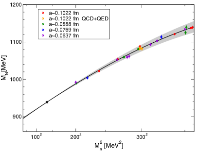
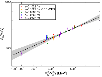
In Fig. 1, we plot our clover determinations of $M_{N}$ versus the values of $M_{\pi}^{2}$ and $M_{K_{\chi}}^{2}$, together with the experimentally measured values for these quantities that define the physical point. We fit these results for $M_{N}$ to various polynomial, Padé and $\chi$PT-motivated functions, of $M_{\pi^{+}}^{2}$ and $M_{K_{\chi}}^{2}$, that include discretization and finite-volume corrections  (?). From each fit we determine the corresponding pair $(F_{\pi^{+}}^{N},F_{K_{\chi}}^{N})$ at the physical point. A similar study of $M_{\pi^{+}}^{2}$ and $M_{K_{\chi}}^{2}$ versus $m_{ud}$ and $m_{s}$ determines the four matrix elements of $J$ at the physical point  (?). Combining these results, as described above, yields the desired $f_{ud}^{N}$ and $f_{s}^{N}$. The statistical errors on these results are calculated using 2000 bootstrap samples. To obtain systematic errors, we consider 6144 different analyses each leading to a result for $f_{ud}^{N}$ and $f_{s}^{N}$ and to a total goodness of fit  (?). These variations are chosen to probe the main sources of systematic error. The results are then combined into distributions whose means give our central values and whose widths determine our systematic errors  (?, ?, ?) (see Table 1). Note that our analysis of the Jacobian also provides a very precise determination of the mass ratio, $m_{s}/m_{ud}=27.29(33)(8)$, where the errors are as in Table 1. From $f_{ud}^{N}$ we further determine the individual $u$ and $d$ contributions to the proton and neutron as in  (?) (see Table 1).

To determine $f_{c}^{N}$, we use 9 staggered ensembles at three $\beta$, corresponding to lattice spacings $a=0.097-0.12\,\mathrm{fm}$. For each $\beta$, the ensembles feature three values of $m_{c}$ equal to $(0.75,1,1.25)$ times the physical value, $m_{c}^{(\phi)}$, with other quark masses held at their physical values. We find that the most reliable way to obtain $f_{c}^{N}$ is to consider the ratios of the nucleon correlator at different $m_{c}$. The exponential fall-off of this ratio gives the difference of $M_{N}$ at these two values of $m_{c}$. From these ratios we get the desired derivative either by a simple Taylor expansion or by a heavy-quark-motivated expansion as detailed in  (?) (see Table 1).

The $b$ and $t$ contributions are determined using the HQ expansions discussed above. Here we use the next-to-next-to-next to leading order result of  (?) to reduce the correction terms to $O\left(\alpha_{s}(m_{b})^{4},(\Lambda_{\mathrm{QCD}}/m_{b})^{2}\right)$, leading to an uncertainty from the HQ expansion of around $0.6\%$  (?). The results are given in Table 1. With the same approach, we can also compute $f_{c}^{N}$. But then the HQ expansion uncertainties on the $c$, $b$ and $t$ contributions becomes $O\left(\alpha_{s}(m_{c})^{4},(\Lambda_{\mathrm{QCD}}/m_{c})^{2}\right)$, i.e. of order $6\%$. We obtain $f_{c}^{N}|_{\text{HQ}}=0.0732(6)(7)$, where the errors are as in Table 1. The difference to the full lattice result is $f_{c}^{N}-f_{c}^{N}|_{\text{HQ}}=0.0002(45)(55)$, in good agreement with the dimensional estimate of the possible HQ corrections, i.e. the HQ expansion works as expected here.

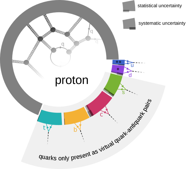
In Fig. 2 we show our results for the $\sigma$-terms of the proton, as fractions of the total proton mass. This representation is renormalization scheme and scale independent, as described in  (?). The $\sigma$-terms of the neutron differ from those of the proton only in the small $u$ and $d$ contributions, at the present level of precision. In addition, we provide a computer code, based on our results, that allows to make predictions and to interpret results of low-energy, experimental searches for new fundamental physics. In particular, using it to sum all contributions, we obtain the low-energy coupling of the Higgs to the nucleon, $f_{hN}=0.3090(58)(61)$, in agreement with, but significantly more precise than the result in  (?).

Beyond its importance for direct dark matter searches and charged-lepton flavor violation, our calculation also allows us to complete the quantitative picture of how protons and neutrons acquire mass, described, for instance, in  (?, ?). Instants after the Big Bang, the universe is a hot gas of elementary particles. Quarks and gluons are massless and interact through the strong interaction with a strength that has been measured at the Large Hadron Collider (LHC). As the universe expands and cools, it undergoes a transition  (?, ?) during which the Higgs field acquires a non-zero expectation value. At that point, elementary fermions get a mass through their interactions with the background Higgs field. As the universe cools down further, in turn top, bottom and charm quarks and antiquarks vanish through decay and annihilation, and subsequently appear only as fleeting quantum fluctuations. The universe can then be described by a theory of the strong interaction in which these particles are completely absent, as long as their fluctuations are subsumed into an increase in the strength of the strong interaction. This is the context in which the calculations of  (?, ?) are performed. As the universe continues to expand, it undergoes another transition, the QCD crossover  (?): the strongly interacting up, down, strange quarks and antiquarks and gluons become confined within bound states. In particular, protons and neutrons form out of up and down quarks, with strange quarks, antiquarks and gluons contributing through fluctuations. As shown in  (?), roughly $95\%$ of the mass of these two bound states comes about due to the energy stored in the quantum fluctuations within them, while less than $5\%$ are induced by the up and down quark masses. The calculation performed here reminds us that, within this $95\%$, $\sum_{q=t,b,c}f_{q}^{N}=21.1(6)\%$ of $M_{N}$ is actually due to quantum fluctuations of the massive $c$, $b$, $t$ quarks, with the remainder being due to gluon and strange quark-antiquark fluctuations. And, as  (?) confirmed, the permil difference between neutron and proton mass arises from a subtle cancellation of electromagnetic effects and effects due to the difference of up and down quark masses.

1 Nucleon scalar couplings

1.1 Feynman-Hellmann theorem

Let $|N(\vec{p},r)\rangle$ be a relativistically-normalized, free nucleon state with three-momentum $\vec{p}$, helicity $r$ and mass $M_{N}$. It is an eigenstate of the renormalized QCD Hamiltonian, $H_{\mathrm{QCD}}=\int d^{3}x\;\mathcal{H}_{\mathrm{QCD}}(x)$ with eigenvalue $E_{\vec{p}}=\sqrt{M_{N}^{2}+\vec{p}^{2}}$. Then, applied to the momentum-independent variation of $H_{\mathrm{QCD}}$ with respect to the renormalizaed mass of quark $q$, $m_{q}^{R}$, the Feynman-Hellmann theorem  (?, ?, ?, ?) implies 

$$\frac{\partial M_{N}^{2}}{\partial m_{q}^{R}}=\frac{1}{2}\sum_{r=1,2}\langle N(\vec{p},r)|\frac{\partial\mathcal{H}_{\mathrm{QCD}}}{\partial m_{q}^{R}}(x)|N(\vec{p},r)\rangle_{c}\ ,$$ (S1)

where the subscript “$c$” indicates that we are referring to the connected part of the matrix element. Now, according to  (?):

$$m_{q}^{R}\frac{\partial\mathcal{H}_{\mathrm{QCD}}}{\partial m_{q}^{R}}(x)=m_{q}^{R}(\bar{q}q)^{R}(x)\ .$$

so that the $\sigma$-terms are given by

$$\sigma^{N}_{q} = \frac{\partial M_{N}}{\partial\ln m_{q}^{R}}$$

$$= \frac{1}{4M_{N}}\sum_{r=1,2}\langle N(\vec{p},r)|m_{q}^{R}(\bar{q}q)^{R}(x)|N(\vec{p},r)\rangle_{c}$$

$$= \langle N|m_{q}\bar{q}q|N\rangle/(2M_{N})\ ,$$

where, in the last line, we introduce a short-hand notation for the previous expression, which takes into account the fact that $m_{q}\bar{q}q$ is renormalization scale and scheme dependent. From this one can define scalar, quark contents:

$$f^{N}_{q}\equiv\frac{\partial\ln M_{N}}{\partial\ln m_{q}^{R}}=\frac{\sigma^{N}_{q}}{M_{N}}$$ (S3)

Note that both the $\sigma-$terms and the quark contents are renormalization scheme and scale independent.

1.2 Nucleon-Higgs coupling in the standard model

In the standard model, the Higgs field $\phi$ obtains a vacuum expectation value

$$\phi_{0}=\frac{v}{\sqrt{2}}=|\langle 0|\phi|0\rangle|\ .$$

The quark masses, like all fundamental fermion masses, originate from a Yukawa term $g_{f}\bar{f}\phi f$ in the fundamental Lagrangian, where $g_{f}$ is that fermion’s Yukawa coupling and the fermion mass is given by

$$m_{f}=g_{f}\phi_{0}\ .$$ (S4)

Expanding $\phi=\phi_{0}+h$ around its vacuum expectation value, it is obvious that the Yukawa term is also responsible for the fermion-Higgs interaction, $g_{f}\bar{f}hf$ which, in principle, can be measured independently. We can thus form the ratio

$$f_{f}=\frac{g_{f}\phi_{0}}{m_{f}}\ ,$$ (S5)

which the standard model predicts to be one for fundamental fermions. A similar ratio can be formed for fundamental gauge bosons and it has been verified experimentally to be one for the $b$ and $t$ quarks, the $\tau$, $W$ and $Z$  (?). We can slightly rewrite this expression by noting that, according to (S4),

$$\frac{\partial m_{f^{\prime}}}{\partial\ln g_{f}}=g_{f}\delta_{ff^{\prime}}\phi_{0}\ ,$$

so that

$$f_{f}^{f^{\prime}}=\frac{\partial\ln m_{f^{\prime}}}{\partial\ln g_{f}}$$ (S6)

is the fraction of the mass of fermion $f^{\prime}$ that couples to the Higgs field via the Yukawa coupling $g_{f}$ .

The advantage of the definition (S6) is that it generalizes naturally. Returning to (S3), we note that the scalar quark content is, in terms of fundamental parameters of the standard model:

$$f^{N}_{q}=\frac{\partial\ln M_{N}}{\partial\ln g_{q}}\ .$$

Thus, it can be interpreted as the mass fraction of the nucleon that couples to the Higgs field via the Yukawa coupling $g_{q}$ of quark $q$. Within the framework of the standard model, one may also interpret $f^{N}_{q}$ as the fraction of the nucleon mass originating from the Higgs field via the Yukawa coupling $g_{q}$. This definition is scale and scheme independent, but it is not unique and we will therefore not pursue it any further.

A large part of the nucleon mass does not couple to the Higgs field via the $g_{q}$. The bulk of this “rest” originates from QCD dynamics and there are standard techniques for decomposing this contribution further  (?, ?, ?). Quantum electrodynamics contributes at the permil level  (?) and there are even smaller contributions due to the weak interaction and the lepton sector, including its coupling to the Higgs. Since the latter two do not take part in the strong interaction, these contributions are suppressed by factors $\alpha^{2}\sim 10^{-4}$ for the lepton sector and $G_{F}\Lambda_{\mathrm{QCD}}^{2}\sim 10^{-5}$ for the weak dynamics respectively. They can safely be ignored at the precision of our current results.

Note that the sum over the scalar quark contents of the nucleon,

$$f^{N}_{h}=\sum_{q}f^{N}_{q}\ ,$$ (S7)

is an observable quantity. It denotes the strength of the coupling of the Higgs to nucleons, in the limit of vanishing momentum transfer. However, measuring it experimentally is a huge challenge, since this requires isolating the highly-suppressed, Higgs exchange contribution to the low-momentum-transfer scattering of a standard model particle off a nucleon. Of course, in Higgs portal dark-matter models, these interactions are the primary detection channel. In other extensions of the standard model, scalar exchange interactions with nucleons may require linear combinations of scalar quark contents that differ from the one given in (S7). For this reason, in Sec. 8 we provide a tool to compute arbitrary linear combinations of quark contents from our results, taking the full correlation matrix into account.

2 Lattice details

Different parts of the analysis rely on different gauge configurations. Some were obtained with a Wilson fermion action and others with a staggered fermion one. These actions were chosen because each has properties that are better suited to different aspects of the calculation.

2.1 Wilson gauge configurations

In order to compute the dependence of the nucleon mass on the meson masses used to interpolate to the physical $u$, $d$ and $s$ quark mass point, we use $N_{f}=4\times 1$, 3HEX-smeared, clover-improved Wilson fermions and a tree-level improved Symanzik gauge action (for details see  (?)). Compared to  (?), two new ensembles were generated at the finest lattice spacing, with strange quark masses significantly differing from the physical value, so as to give us a larger lever arm in the strange quark mass direction. The full list of these ensembles is provided in Table S1.

$6/g^{2}$	$e$	$am_{u}$	$am_{d}$	$am_{s}$	$L^{3}\times T$	$m_{\pi}[\mathrm{MeV}]$	$m_{\pi}L$	$\times 1000$ trajectories
3.2	0	-0.0686	-0.0674	-0.068	$32^{3}\times 64$	413	6.9	1
3.2	0	-0.0737	-0.0723	-0.058	$32^{3}\times 64$	353	5.9	4
3.2	0	-0.0733	-0.0727	-0.058	$32^{3}\times 64$	356	5.8	1
3.2	0	-0.0776	-0.0764	-0.05	$32^{3}\times 64$	294	4.9	4
3.2	0	-0.0805	-0.0795	-0.044	$32^{3}\times 64$	238	4.0	12
3.2	0	-0.0806	-0.0794	-0.033	$32^{3}\times 64$	266	4.4	12
3.2	0	-0.0686	-0.0674	-0.02	$32^{3}\times 64$	488	8.1	4
3.2	0	-0.0737	-0.0723	-0.025	$32^{3}\times 64$	411	6.8	4
3.2	0	-0.0776	-0.0764	-0.029	$32^{3}\times 64$	336	5.6	4
3.2	0	-0.077	-0.0643	-0.0297	$32^{3}\times 64$	438	7.3	4
3.2	0	-0.073	-0.0629	-0.0351	$32^{3}\times 64$	469	7.8	4
3.2	0	-0.077	-0.0669	-0.0391	$32^{3}\times 64$	405	6.7	4
3.2	1.00	-0.0859	-0.0792	-0.0522	$24^{3}\times 48$	298	3.7	5
3.2	1.00	-0.0859	-0.0792	-0.0522	$32^{3}\times 64$	295	4.9	4
3.2	1.00	-0.0859	-0.0792	-0.0522	$48^{3}\times 96$	295	7.3	4
3.2	1.00	-0.0859	-0.0792	-0.0522	$80^{3}\times 64$	295	12.2	1
3.3	0	-0.0486	-0.0474	-0.048	$32^{3}\times 64$	422	6.1	1
3.3	0	-0.0537	-0.0523	-0.038	$32^{3}\times 64$	348	5.1	2
3.3	0	-0.0535	-0.0525	-0.038	$32^{3}\times 64$	349	5.0	2
3.3	0	-0.0576	-0.0564	-0.03	$32^{3}\times 64$	275	4.0	12
3.3	0	-0.0576	-0.0564	-0.019	$32^{3}\times 64$	293	4.2	12
3.3	0	-0.0606	-0.0594	-0.024	$48^{3}\times 64$	200	4.3	20
3.4	0	-0.034	-0.033	-0.0335	$32^{3}\times 64$	403	5.0	4
3.4	0	-0.0385	-0.0375	-0.0245	$32^{3}\times 64$	321	4.0	4
3.4	0	-0.0423	-0.0417	-0.0165	$48^{3}\times 64$	219	4.1	4
3.5	0	-0.0218	-0.0212	-0.0215	$32^{3}\times 64$	426	4.4	4
3.5	0	-0.0254	-0.0246	-0.0145	$48^{3}\times 64$	348	5.4	4
3.5	0	-0.0268	-0.0262	-0.0115	$48^{3}\times 64$	310	4.8	8
3.5	0	-0.0269	-0.0261	-0.0031	$48^{3}\times 64$	317	4.9	8
3.5	0	-0.0285	-0.0275	-0.0085	$48^{3}\times 64$	266	4.1	8
3.5	0	-0.0302	-0.0294	-0.0049	$64^{3}\times 96$	199	4.1	4
3.5	0	-0.027	-0.027	-0.027	$48^{3}\times 64$	280	4.4	3
3.5	0	-0.028	-0.028	+0.009	$48^{3}\times 64$	282	4.4	3.5

Table S1: List of 3HEX clover ensembles used to determine the meson-mass dependence of the proton mass.

2.2 Determination of hadron masses on Wilson ensembles

We mainly use the pure QCD ($e=0$) ensembles. Pseudoscalar meson masses, $M_{P}$ are determined from a fit to multiple, zero-three-momentum correlators with a common value of $M_{P}$:

$$C_{PP}(t)=\langle P(t)P^{\dagger}(0)\rangle\qquad\mbox{and}\qquad C_{A_{0}P}(t)=\langle A_{0}(t)P^{\dagger}(0)\rangle\ ,$$ (S8)

with $P=\bar{q}\gamma_{5}q^{\prime}$, $A_{0}=\bar{q}\gamma_{0}\gamma_{5}q^{\prime}$ and $q$ and $q^{\prime}$ are distinct quark flavors chosen amongst $u$, $d$ and $s$. We fit these correlation functions to

$$C_{PP}(t)=d\cosh(M_{P}(t-T/2))\qquad\mbox{and}\qquad C_{A_{0}P}(t)=f\sinh(M_{P}(t-T/2))\ ,$$ (S9)

where $T$ is the lattice temporal extent. Nucleon correlation functions are those of  (?). The corresponding masses were obtained by fits to single, decaying exponentials.

Fit ranges are five lattice spacings long and the initial time slices, $t_{i}$, are matched, on different ensembles, to have a constant ratio between estimated excited-state effects and the relative, statistical error on the nucleon mass. Specifically, we take the smallest $t_{i}>t_{0}-\ln(\epsilon_{i})/\Delta M$, where $\epsilon_{i}$ is the statistical error of the nucleon mass extracted with initial time slice $t_{i}$, $\Delta M=500\,\mathrm{Me\kern-1.00006ptV}$ is an estimate of the mass difference to the first excited nucleon state and $t_{0}$ is a parameter which we vary in our analysis from $-1.4\,\mathrm{fm}$ to $-1.25\,\mathrm{fm}$ .

$t_{0}$	KS prob. $M_{p}$	KS prob. $M_{n}$
-1.40	0.59	0.86
-1.35	0.87	0.99
-1.30	0.54	0.85
-1.25	0.32	0.60

Table S2: The Kolmogorov-Smirnov probability of the CDF of the proton and neutron mass fit qualities compared to a uniform distribution for various values of the offset $t_{0}$ (see text).

Table S2 lists the Kolmogorov-Smirnov (KS) probabilities from a comparison of the CDFs of the nucleon mass fit qualities to a uniform distribution as detailed in  (?). KS probabilities for the multi-channel meson fits are around $0.2$ because of their highly correlated nature. Fitting channels individually however gives fully compatible results and KS probabilities that are in the same range as those for $M_{p}$ and $M_{n}$. Therefore, we are confident that, by considering the full range of offset values, $t_{0}$, from Table S2 we obtain a conservative estimate of remnant excited state effects.

For the extrapolation to the physical point, we used the ensembles reported in Table S1. To get a better handle on the finite-volume dependence of the nucleon mass, we added the four $e=1$, $\beta=3.2$ ensembles at $M_{\pi}\sim 290\,\mathrm{Me\kern-1.00006ptV}$ that differ only in their volume $L^{3}\times T$, with $L\in\{24,32,48,80\}$, compared to our set of pure QCD ensembles. Since these ensembles were tuned to the isospin symmetric point, we can use the neutron mass instead of the nucleon mass, the connected-pseudoscalar-meson mass average, $(M_{uu}^{2}+M_{dd}^{2})/2$, instead of $M_{\pi}^{2}$ and $2M_{K^{0}}^{2}-M_{dd}^{2}$ instead of $M_{K_{\chi}}^{2}$.

2.3 Staggered gauge configurations and correlation functions

We use staggered ensembles near the physical point to extract the dependence of the pseudoscalar meson masses, $M_{P}$, on the quark masses, $m_{q}$. The full list of these ensembles used in the analysis is provided in Table S3.

$6/g^{2}$	$am_{ud}$	$am_{s}$	$am_{c}$	$L^{3}\times T$	$m_{\pi}L$	$\times 1000$ trajectories
3.84	0.00151556	0.0431935	0.511843	$64^{3}\times 96$	4.1	5.1
3.84	0.00151556	0.04015	.4757775	$64^{3}\times 96$	4.1	3.25
3.84	0.00143	.0431935	.511843	$64^{3}\times 96$	4.0	3.2
3.84	0.001455	.04075	.4828875	$64^{3}\times 96$	4.1	15
3.84	0.001455	.04075	.4665875	$64^{3}\times 96$	4.0	3.1
3.84	0.001455	.03913	.4636905	$64^{3}\times 96$	4.0	5
3.92	0.001207	0.032	0.3792	$80^{3}\times 128$	4.2	10
3.92	0.0012	0.0332856	0.39443436	$80^{3}\times 128$	4.2	14.5
4.0126	0.000958973	0.0264999	0.314023	$96^{3}\times 144$	4.1	1
4.0126	0.000977	.0264999	0.314023	$96^{3}\times 144$	4.2	10
4.0126	0.001002	0.027318	0.323716	$96^{3}\times 144$	4.2	2.7

Table S3: List of 4stout smeared staggered ensembles used to compute the quark-mass dependence of the pseudoscalar meson masses.

The Goldstone-pion mass is close to the physical one in all of these ensembles. The volumes are matched and $M_{\pi}L>4$, which implies that the finite-volume corrections to the pion mass and decay constant are below the permil level  (?). The kaon mass and decay constant receive even smaller corrections. Since we do not determine any other observables from these configurations, an infinite-volume extrapolation is not necessary in this part of the analysis. Further details on the action used can be found in  (?, ?).

The dependence of the nucleon mass on the charm quark mass is obtained directly from a set of nine 4-stout-smeared staggered ensembles (“charm ensembles”), at three values of $\beta=3.75$, $3.7753$, $3.84$. At each $\beta$ one ensemble, which we call the central ensemble, was tuned to the physical point with a deviation of less then 4 % in $M^{2}_{\pi}/f^{2}_{\pi},(2M^{2}_{K}-M_{\pi}^{2})/f^{2}_{\pi}$ and the bare charm quark mass was set to $11.85$ times the bare strange-quark mass  (?). Two other ensembles were obtained from each central ensemble by varying the bare charm-quark mass to $1.25$ and $0.75$ times the value on the central ensemble and leaving all other parameters fixed. In each of these 9 ensembles, we have generated 64 configurations separated by $10$ trajectories each.

The sources and corresponding propagators are the standard ones provided, for instance, by the MILC code  (?).

2.4 Determination of hadron masses on the staggered ensembles

For the ensembles in Table S3, we obtain pseudoscalar masses and decay constants from fits to the pseudoscalar propagators starting at a fixed (in physical units) $t_{\mathrm{min}}=1.9\,\mathrm{fm}$ or $t_{\mathrm{min}}=2.3\,\mathrm{fm}$. Fit ranges are ten lattice spacings long. In Table S4 we list the KS probabilities that result from comparing the CDFs of the pion and kaon fit qualities to a uniform random distribution.

$t_{\mathrm{min}}[\mathrm{fm}]$	KS prob. $M_{\pi}$	KS prob. $M_{K}$
1.9	0.87	0.33
2.3	0.14	0.77

Table S4: Kolmogorov-Smirnov probability of the CDF of the pion and of the kaon mass fit qualities compared to a uniform distribution for various values of the offset $t_{\mathrm{min}}$.

To extract masses from a staggered propagator, $c_{t}$, we either use a standard staggered two state fit or, alternatively, we construct a time-shifted propagator:

$$d_{t}(M)\equiv c_{t}+e^{M}c_{t+1}$$ (S10)

The time-shifted propagator is useful if there is a region in $t$ with negligible backward contributions, $m(T/2-t)\gg 1$, and negligible excited states except the parity partner of the nucleon. Here $m$ is the ground state mass and $T$ the lattice temporal extent. The staggered propagator in this region behaves as

$$c_{t}=e^{-mt}\left(c_{0}+(-1)^{t}c_{1}e^{-\Delta t}\right)\ ,$$ (S11)

with the mass difference to the staggered parity partner, $\Delta$, and the matrix elements $c_{0}$ and $c_{1}$ of the ground state and staggered parity partner, respectively.

The contribution of the staggered parity partner to the time-shifted propagator (S10) can, in principle, be cancelled out by setting $M=m+\Delta$:

$$d_{t}(m+\Delta)=c_{0}e^{-mt}(1+e^{\Delta})\ .$$ (S12)

We can determine $M$ self-consistently by defining a local effective mass

$$l_{t}(M)\equiv\ln(d_{t}(M)/d_{t+1}(M))\ ,$$ (S13)

as well as its average,

$$\bar{l}(M)=\frac{1}{n}\sum_{t=0}^{t_{0}+n-1}l_{t}(m)$$ (S14)

in the signal region, $t_{0}\leq t\leq t_{0}+n$, and by minimizing

$$\sum_{t_{1},t_{2}=0}^{t_{0}+n-1}(l_{t_{1}}(M)-\bar{l}(M))(C^{-1})_{t_{1}t_{2}}(l_{t_{2}}(M)-\bar{l}(M))$$ (S15)

with respect to $M$, where $C$ is the correlation matrix corresponding to $l_{t}(M)-\bar{l}(M)$. The resulting parameter is $M_{\mathrm{opt}}$ and we call the corresponding propagator, $d_{t}(M_{\mathrm{opt}})$, the optimal time-shifted propagator.

It is important to note that $M_{\mathrm{opt}}$ is just one number per ensemble that fixes the relative contributions of $c_{t}$ and $c_{t+1}$ in the time-shifted propagator. In particular, it does not directly enter any further stages of analysis. After having determined $M_{\mathrm{opt}}$, we proceed to extract the ground state mass from $d_{t}(M_{\mathrm{opt}})$ in a standard fashion. In fact, the time-shifted propagator $d_{t}(M)$ does have the correct asymptotic time behavior for any constant $M$ and thus an inaccurate determination of $M_{\mathrm{opt}}$ does not invalidate the ground-state-mass extraction from $d_{t}(M_{\mathrm{opt}})$. If cancellation of the staggered parity partner is not achieved to within the statistical accuracy of the correlator, or additional excited states or backward contributions are present, the consequent fit to determine the ground state mass from $d_{t}(M_{\mathrm{opt}})$ will simply fail with a bad fit quality.

On our charm ensembles, we determine mass differences from ratios of optimal time-shifted propagators. The plateau length is always 8 lattice spacings and the plateau start is either $t_{\mathrm{min}}=0.8\,\mathrm{fm}$ or $t_{\mathrm{min}}=1.0\,\mathrm{fm}$.

3 Computing mesonic $\sigma$-terms

We determine the dependence of the nucleon mass on the pseudoscalar meson masses from our 3HEX ensembles (Table S1). We define the isospin symmetric physical point of QCD by $M_{N}=(M_{p}+M_{n})/2=938.919\,\mathrm{Me\kern-1.00006ptV}$  (?) and $M_{\pi}=134.8\,\mathrm{Me\kern-1.00006ptV},M_{K_{\chi}}=685.8\,\mathrm{Me\kern-1.00006ptV}$  (?). In order to estimate the dependence of our result on the range of the chiral expansion, we imposed two different cuts on the maximal pion mass $M_{\pi}\leq 360/420\,\mathrm{Me\kern-1.00006ptV}$ entering our analysis.

3.1 Fit forms

The nucleon mass is extrapolated to the physical point with an ansatz

$$M_{N}=M_{N}^{\phi}\times\prod_{i}\left(1+c_{i}(v_{i}-v_{i}^{(\phi)})\right)^{t_{i}}\ ,$$ (S16)

where the $c_{i}$ are the fit parameters, $v_{i}$ the fit variables, $t_{i}=\pm 1$ (Taylor/Padé) and generically $x^{(\phi)}$ denotes the physical value of the observable $x$. We perform fits to functions that all contain the pseudoscalar mass dependencies $v_{1}=M_{\pi}^{2}$, with $t_{1}=1$, and $v_{2}=M_{K_{\chi}}^{2}$, with either $t_{2}=\pm 1$. They also include the finite-volume term $v_{3}=M_{\pi}^{1/2}L^{-3/2}e^{-M_{\pi}L}$, with $t_{3}=1$. In addition, they contain either of the two next-to-leading-order terms in $M_{\pi}^{2}$, namely $v_{4}=M_{\pi}^{3}$ with $t_{4}=1$, or $v_{5}=M_{\pi}^{4}$ with $t_{5}=1$, corresponding to either a chiral or generic Taylor expansion in $M_{\pi}^{2}$  (?). They further include either no discretization term or the formally leading discretization terms $v_{6}=\alpha_{s}a(M_{\pi}^{2}-M_{\pi}^{(\phi)2})$ with $t_{6}=1$ and $v_{7}=\alpha_{s}a(M_{K_{\chi}}^{2}-M_{K_{\chi}}^{(\phi)2})$ with $t_{7}=1$; or the formally subleading $v_{8}=a^{2}(M_{\pi}^{2}-M_{\pi}^{(\phi)2})$, $t_{8}=1$, and $v_{9}=a^{2}(M_{K_{\chi}}^{2}-M_{K_{\chi}}^{(\phi)2})$, $t_{9}=1$  (?). Note that we set the scale with $M_{N}$, so that discretization terms proportional to just $\alpha_{s}a$ or $a^{2}$ would be redundant.

3.2 Systematic error variations

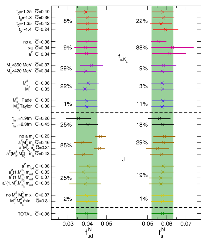
The total number of distinct analyses is 4(plateau ranges)$\times$2($M_{\pi}$ cut)$\times$2(chiral/Taylor expansion in $M_{\pi}^{2}$)$\times$2(Taylor/Padé in $M_{K_{\chi}}^{2}$)$\times$3(discretization)$=96$. The way in which we combine these analyses to give a final central value and systematic error is described in Sec. 3.4. In Fig. S1 we present the variation of our final observables, $f_{ud}^{N}$ and $f_{s}^{N}$, that result from applying these different fit procedures. Results from all different fit procedures are in good agreement. The leading sources of systematic error come from the continuum limit and the pion mass cuts.

Figure S1: Variation of $f_{ud}^{N}$ and $f_{s}^{N}$ from different restrictions on the full analysis procedure. The top part of the panel corresponds to variations in the determination of the meson mass dependence of the nucleon mass. From top to bottom these are: restriction to a single plateau range, to a single scaling behavior, to a single pion cut, to either Taylor or chiral expansion in $M_{\pi}^{2}$ and to Taylor or Padé expansion in $M_{K_{\chi}}^{2}$. The middle part displays the effect of variations in the computation of the elements of the mixing matrix $J$. From top to bottom these are: restriction to a single plateau range, to a single continuum fit form for $m_{s}$, to a single continuum fit form for $m_{ud}$ and to the inclusion/exclusion of crossterms in the $m_{ud}$, $m_{s}$ and scale setting fits. The last row shows the final result including all fits. The average fit quality of the analyses $\bar{Q}$ is given in each case. The percentage of the total systematic error due to each variation alone is also displayed (percentages add up to $1$ in quadrature).

3.3 Crosschecks

From the nucleon fits we can extract the lattice spacings, which are reported in Table S5. A comparison to  (?), where $M_{\Omega}$ was used to set the scale on a set of ensembles which has a large overlap with the current one, reveals perfect agreement.

$\beta$	$a[\mathrm{fm}]$
3.2	0.1022(6)(8)
3.3	0.0888(5)(5)
3.4	0.0769(5)(4)
3.5	0.0637(3)(3)

Table S5: Lattice spacings obtained from the nucleon fit. Here and throughout the paper the first error is statistical and the second, the total systematic error, unless stated otherwise.

To check the validity of our finite-volume ansatz, we verified that the fit coefficient $c_{3}=35(13)(5)\mathrm{GeV}^{-2}$ is compatible with the numerical predictions of  (?). To further investigate possible finite-volume effects beyond the leading order, we performed two complete auxiliary analyses with explicit pion finite-volume effects according to  (?), one with fixed and one with fitted prefactors. The influence on central values and errors was found to be insignificant and, in the case of the fitted prefactor, the additional term was found to be compatible with zero.

Figure S2: Lattice-spatial-extent dependence of the nucleon mass in one sample fit. The fit has been used to shift the simulation results to the physical point in all of the other variables on which these results depend.

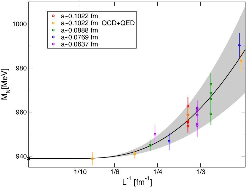
3.4 Results

The nucleon fits have fit qualities in the range $Q=0.07-0.38$, with an average fit quality $\bar{Q}=0.23$. In Figs. 1 and S2 we display, for one sample fit, the dependence of the nucleon mass on $M_{\pi}^{2}$, $M_{K_{\chi}}^{2}$ and the inverse of the spatial lattice extent $L$. Defining pion and reduced kaon $\sigma$-terms as,

$$\sigma_{\pi N}=M_{\pi}^{2}\left.\frac{\partial M_{N}}{\partial M_{\pi}^{2}}\right|_{M_{K_{\chi}}}\qquad\mbox{and}\qquad\sigma_{K_{\chi}N}=M_{K_{\chi}}^{2}\left.\frac{\partial M_{N}}{\partial M_{K_{\chi}}^{2}}\right|_{M_{\pi}}\ ,$$ (S17)

we obtain $\sigma_{\pi N}=42.0(1.3)(1.4)\,\mathrm{Me\kern-1.00006ptV}$ and $\sigma_{K_{\chi}N}=50.9(3.3)(2.8)\,\mathrm{Me\kern-1.00006ptV}$. We also define the logarithmic derivatives,

$$F_{\pi}^{N}=\frac{\sigma_{\pi N}}{M_{N}}=\left.\frac{\partial\ln M_{N}}{\partial\ln M_{\pi}^{2}}\right|_{M_{K_{\chi}}}\qquad\mbox{and}\qquad F_{K_{\chi}}^{N}=\frac{\sigma_{K_{\chi}N}}{M_{N}}=\left.\frac{\partial\ln M_{N}}{\partial\ln M_{K_{\chi}}^{2}}\right|_{M_{\pi}}\ ,$$ (S18)

for which our final results are $F_{\pi}^{N}=0.0447(14)(15)$ and $F_{K_{\chi}}^{N}=0.0542(36)(29)$. From these fits we also obtain an estimate of the nucleon mass at vanishing $M_{\pi}$ keeping $M_{K_{\chi}}$ fixed, $\left.M_{N}\right|_{M_{\pi}=0}=896(1)(2)\,\mathrm{Me\kern-1.00006ptV}$, and, conversely, an estimate of the nucleon mass at vanishing $M_{K_{\chi}}$ keeping $M_{\pi}$ fixed, $\left.M_{N}\right|_{M_{K_{\chi}}=0}=889(3)(3)\,\mathrm{Me\kern-1.00006ptV}$. These results, as well as our value for the nucleon mass in the $SU(3)$ chiral limit $\left.M_{N}\right|_{M_{\pi}=M_{K_{\chi}}=0}=848(3)(3)\,\mathrm{Me\kern-1.00006ptV}$, should be interpreted with great care, since it is not clear that our interpolation and extrapolation functions are valid down to vanishing quark masses.

4 Relation between quark and meson masses

To leading order in chiral perturbation theory, $M_{\pi}^{2}$ and $M_{K_{\chi}}^{2}$ are proportional to $m_{ud}$ and $m_{s}$. The logarithmic derivatives $F_{\pi}^{N}$ and $F_{K_{\chi}}^{N}$ defined in (S18) are therefore equal to the nucleon quark content,

$$f_{ud}=\left.\frac{\partial\ln M_{N}}{\partial\ln m_{ud}}\right|_{m_{s}}\qquad\mbox{and}\qquad f_{s}=\left.\frac{\partial\ln M_{N}}{\partial\ln m_{s}}\right|_{m_{ud}}$$ (S19)

in leading order. To go beyond leading order, we need to determine the relation between pseudoscalar meson masses and quark masses around the physical point. For this purpose we use the $N_{f}=2+1+1$ staggered ensembles presented in Sec. 2.3, which bracket the physical point.

4.1 The Jacobian matrix

Transforming the $F_{P}^{N}$, $P\in\{\pi,K_{\chi}\}$ into the $f_{q}$, $q\in\{ud,s\}$ is achieved via the Jacobian matrix, $J$, with elements

$$J_{P,q}=\frac{\partial\ln M_{P}^{2}}{\partial\ln m_{q}}\ ,$$ (S20)

evaluated at the physical point so that

$$f_{q}=\frac{\partial\ln M_{N}}{\partial\ln m_{q}}=\sum_{P}\frac{\partial\ln M_{N}}{\partial\ln M_{P}^{2}}J_{P,q}=\sum_{P}F_{P}^{N}J_{P,q}\ .$$ (S21)

While the $F_{P}^{N}$ are defined at the physical point, including the charm quark mass, the $N_{f}=2+1+1$ ensembles, on which we calculate the Jacobian, are at a variety of different charm quark masses. Thus, when discussing the Jacobian, we are careful about recording $m_{c}$ dependence. Since the computation of this Jacobian is best done with staggered fermions, whose masses are multiplicatively renormalized, we parametrize this dependence by the ratio $r_{cs}=m_{c}/m_{s}$, where renormalization factors cancel in mass-independent schemes. Then we fit the light and strange quark mass as functions of $M_{\pi}^{2}$, $M_{K_{\chi}}^{2}$ and $r_{cs}$:

$$m_{ud}(M_{\pi}^{2},M_{K_{\chi}}^{2},r_{cs})\qquad\mbox{and}\qquad m_{s}(M_{\pi}^{2},M_{K_{\chi}}^{2},r_{cs})\ .$$ (S22)

From these fit functions, we determine the following logarithmic derivatives at the physical point:

$$N_{q,\pi}=\left.\frac{\partial\ln m_{q}}{\partial\ln M_{\pi}^{2}}\right|_{M_{K_{\chi}}^{2},r_{cs}}\ ,\quad N_{q,K_{\chi}}=\left.\frac{\partial\ln m_{q}}{\partial\ln M_{K_{\chi}}^{2}}\right|_{M_{\pi}^{2},r_{cs}}\ ,\quad N_{q,r}=\left.\frac{\partial\ln m_{q}}{\partial\ln r_{cs}}\right|_{M_{\pi},M_{K_{\chi}}^{2}}\ .$$ (S23)

In principle we need to compute the Jacobian between the two sets of parameters $(M_{\pi}^{2},M_{K_{\chi}}^{2},r_{cs})$ and $(m_{ud},m_{s},m_{c})$. However, the elements of the Jacobian matrix that we are ultimately interested in are those at fixed $m_{c}$, i.e.

$$J_{P,ud}=\left.\frac{\partial\ln M_{P}^{2}}{\partial\ln m_{ud}}\right|_{m_{s},m_{c}}\qquad\mbox{and}\qquad J_{P,s}=\left.\frac{\partial\ln M_{P}^{2}}{\partial\ln m_{s}}\right|_{m_{ud},m_{c}}\ .$$ (S24)

They are obtained from (S23) as

$$\begin{split}J_{\pi,ud}&=\frac{N_{s,K_{\chi}}}{N_{ud,\pi}N_{s,K_{\chi}}-N_{ud,K_{\chi}}N_{s,\pi}}\ ,\\ J_{\pi,s}&=-\frac{N_{ud,K_{\chi}}(1-N_{s,r})-N_{s,K_{\chi}}N_{ud,r}}{N_{ud,\pi}N_{s,K_{\chi}}-N_{ud,K_{\chi}}N_{s,\pi}}\ ,\\ J_{K_{\chi},ud}&=-\frac{N_{s,\pi}}{N_{ud,\pi}N_{s,K_{\chi}}-N_{ud,K_{\chi}}N_{s,\pi}}\ ,\\ J_{K_{\chi},s}&=\frac{N_{ud,\pi}(1-N_{s,r})-N_{s,\pi}N_{ud,r}}{N_{ud,\pi}N_{s,K_{\chi}}-N_{ud,K_{\chi}}N_{s,\pi}}\ .\end{split}$$ (S25)

4.2 Renormalization

The matrix $J$ is a scheme and scale independent quantity. Each element has the form of $m_{q}/M_{P}^{2}\times\partial M_{P}^{2}/\partial m_{q}$, where $m_{q}$ is a quark mass and $M_{P}$, either $M_{\pi^{+}}$ or $M_{K_{\chi}}$. Any multiplicative renormalization factor cancels in these ratios provided that it is independent of the quark masses. However, to allow for a global fit of $m_{ud}$ and $m_{s}$ to the functions of (S22), involving ensembles with different lattice spacings, a specific scheme has to be introduced. We chose the simplest possible scheme: fixing the value of the renormalized strange quark mass at the physical point to a constant independent of quark masses and lattice spacing. The exact procedure is detailed in Sec. 4.3

4.3 Fit functions

In order to set the scale, we interpolate the pion decay constant, $f_{\pi}$, to the physical mass point defined by the physical values, $M_{\pi}^{(\phi)2}$ and $M_{K_{\chi}}^{(\phi)2}$, of the squared pion and reduced kaon masses, and by $r_{cs}^{(\phi)}$, which we set to $11.85$. Since all of our results are dimensionless ratios, scale setting is not critical and especially a variation in $r_{cs}^{(\phi)}$ has negligible effect on the result. Varying the interpolation function has no effect on our results as is evident from Fig. S1.

To determine $J$ we study the behavior of the functions $m_{ud}(M_{\pi}^{2},M_{K_{\chi}}^{2},r_{cs})$ and $m_{s}(M_{\pi}^{2},$ $M_{K_{\chi}}^{2}$, $r_{cs})$. We expand these around the physical mass point, again defined by $M_{\pi}^{(\phi)2}$, $M_{K_{\chi}}^{(\phi)2}$ and $r_{cs}^{(\phi)}$. The fit functions we employ have the form

$$m_{ud}^{R}(M_{\pi}^{2},M_{K_{\chi}}^{2},r_{cs})=c_{00}^{ud}+c_{10}^{ud}\Delta_{\pi}+c_{01}^{ud}\Delta_{K_{\chi}}+c_{20}^{ud}\Delta_{\pi}^{2}+c_{02}^{ud}\Delta_{K_{\chi}}^{2}+c_{11}^{ud}\Delta_{\pi}\Delta_{K_{\chi}}+c_{c1}^{ud}\Delta_{r_{cs}}$$ (S26)

and

$$m_{s}^{R}(M_{\pi}^{2},M_{K_{\chi}}^{2},r_{cs})=c_{00}^{s}+c_{10}^{s}\Delta_{\pi}+c_{01}^{s}\Delta_{K_{\chi}}+c_{20}^{s}\Delta_{\pi}^{2}+c_{02}^{s}\Delta_{K_{\chi}}^{2}+c_{11}^{s}\Delta_{\pi}\Delta_{K_{\chi}}+c_{c1}^{s}\Delta_{r_{cs}}\ ,$$ (S27)

where $\Delta_{\pi}=M_{\pi}^{2}-M_{\pi}^{(\phi)2}$, $\Delta_{K_{\chi}}=M_{K_{\chi}}^{2}-M_{K_{\chi}}^{(\phi)2}$, $\Delta_{r_{cs}}=r_{cs}-r_{cs}^{(\phi)}$ and $m_{q}^{R}$ are renormalized quark masses. They are related to the bare quark masses $m_{q}$, which are parameters of the action, by a multiplicative renormalization factor, $Z$, so that $m_{ud}^{R}=Zm_{ud}(M_{\pi}^{2},M_{K_{\chi}}^{2},r_{cs})$ and $m_{s}^{R}=Zm_{s}(M_{\pi}^{2},M_{K_{\chi}}^{2},r_{cs})$. We choose a scheme in which the renormalization factors do not depend on the quark masses, and consequently the squared pion and reduced kaon masses, but only on the gauge coupling $\beta$. To avoid an explicit determination of the renormalization factors, we divide the above expansions by the value of the renormalized strange quark mass at the physical mass point for each $\beta$, yielding:

$$\frac{m_{ud}(M_{\pi}^{2},M_{K_{\chi}}^{2},r_{cs})}{m_{s}(M_{\pi}^{(\phi)2},M_{K_{\chi}}^{(\phi)2},r_{cs}^{(\phi)})}=r+d_{10}^{ud}\Delta_{\pi}+d_{01}^{ud}\Delta_{K_{\chi}}+d_{20}^{ud}\Delta_{\pi}^{2}+d_{02}^{ud}\Delta_{K_{\chi}}^{2}+d_{11}^{ud}\Delta_{\pi}\Delta_{K_{\chi}}+d_{c1}^{ud}\Delta_{r_{cs}}$$ (S28)

and

$$\frac{m_{s}(M_{\pi}^{2},M_{K_{\chi}}^{2},r_{cs})}{m_{s}(M_{\pi}^{(\phi)2},M_{K_{\chi}}^{(\phi)2},r_{cs}^{(\phi)})}=1+d_{10}^{s}\Delta_{\pi}+d_{01}^{s}\Delta_{K_{\chi}}+d_{20}^{s}\Delta_{\pi}^{2}+d_{02}^{s}\Delta_{K_{\chi}}^{2}+d_{11}^{s}\Delta_{\pi}\Delta_{K_{\chi}}+d_{c1}^{s}\Delta_{r_{cs}}\ ,$$ (S29)

where $r$ is the ratio of the strange and to light quark mass at the physical point and $d_{ij}^{q}=c_{ij}^{q}/m_{s}(M_{\pi}^{(\phi)2},M_{K_{\chi}}^{(\phi)2},r_{cs}^{(\phi)})$, for $q=ud,s$ and for all values of $ij$ appearing in Eqs. (S28) and (S29). Note that all renormalization factors cancel out. The value $m_{s}(M_{\pi}^{(\phi)2},M_{K_{\chi}}^{(\phi)2},r_{cs}^{(\phi)})$ is different for each gauge coupling $\beta$. This is a manifestation of the need for renormalization. In practice, we introduce fit parameters $m_{s}^{(\phi)}[\beta]$, where $\beta$ in rectangular brackets indicates that one independent parameter per gauge coupling is considered.

The above expansions are subject to discretization artefacts. We consider these to contribute to the ratio $r$ and to the linear terms in $\Delta_{\pi}$ and $\Delta s$. Discretization artefacts on the quadratic terms are subleading. The final fit functions are

$$\frac{m_{ud}(M_{\pi}^{2},M_{K_{\chi}}^{2},r_{cs})}{m_{s}^{(\phi)}[\beta]} = r_{0}+a^{2}r_{1}+(d_{10}^{ud}+e_{10}^{ud}a^{2})\Delta_{\pi}+(d_{01}^{ud}+e_{01}^{ud}a^{2})\Delta_{K_{\chi}}+$$ (S30)

$$d_{20}^{ud}\Delta_{\pi}^{2}+d_{02}^{ud}\Delta_{K_{\chi}}^{2}+d_{11}^{ud}\Delta_{\pi}\Delta_{K_{\chi}}+d_{c1}^{ud}\Delta_{r_{cs}}$$

and

$$\frac{m_{s}(M_{\pi}^{2},M_{K_{\chi}}^{2},r_{cs})}{m_{s}^{(\phi)}[\beta]} = 1+(d_{10}^{s}+e_{10}^{s}a^{2})\Delta_{\pi}+(d_{10}^{s}+e_{10}^{s}a^{2})\Delta_{K_{\chi}}+$$ (S31)

$$d_{20}^{s}\Delta_{\pi}^{2}+d_{02}^{s}\Delta_{K_{\chi}}^{2}+d_{11}^{s}\Delta_{\pi}\Delta_{K_{\chi}}+d_{c1}^{s}\Delta_{r_{cs}}.$$

We perform various fits, all of which contain the fit parameters $r_{0}$, $r_{1}$, $d_{10}^{q},d_{01}^{q}$ and $d_{c1}^{q}$. The discretization terms $e_{10}^{q}$, $e_{01}^{q}$ and the higher order interpolation terms $d_{11}^{q}$ are optionally present and we perform fits with all possible variations, with each term either present or absent. The additional, higher-order terms, $d_{20}^{q}$ and $d_{02}^{q}$, turn out to be irrelevant and can be omitted entirely.

Finite-volume effects on all relevant quantities are safely below 1 permil on all of our ensembles  (?) and cannot be detected with the statistical accuracy of our data.

Figure S3: Dependence of the quark masses, $m_{ud}$ and $m_{s}$, on the squared pseudoscalar-meson masses, $M_{\pi}^{2}$ and $M_{K_{\chi}}^{2}$, for one of our analyses. Data points are corrected using the fit to tune all, except the plotted variables, to their physical value.

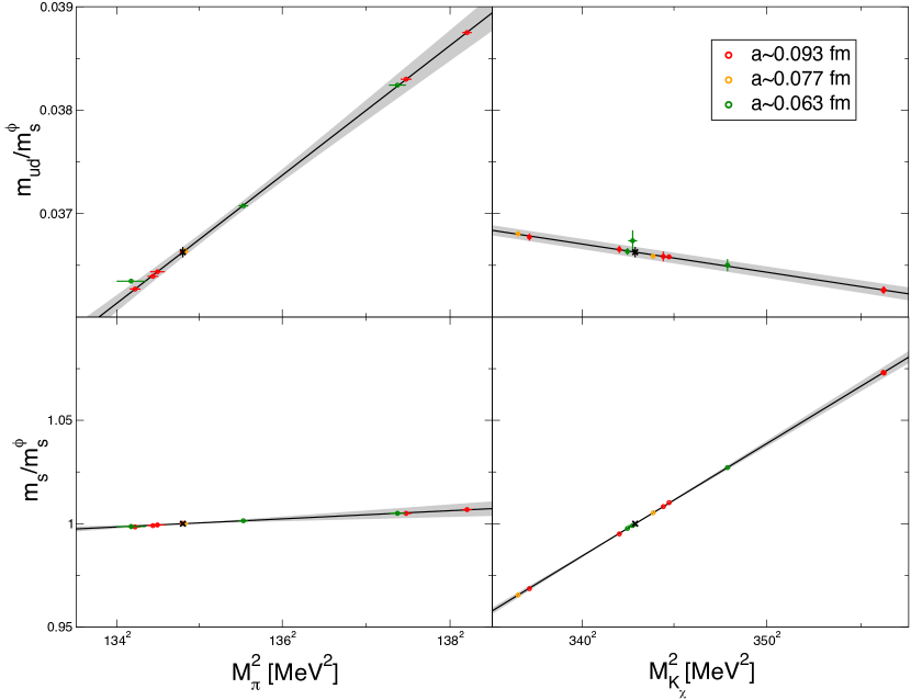
The $M_{\pi}^{2}$ and $M_{K_{\chi}}^{2}$ dependence of the quark masses for a single representative analysis are displayed in Fig. S3.

4.4 Systematic error variations

The total number of distinct analyses for the Jacobi matrix is 2(plateau ranges) $\times$ 4(discretization terms on $m_{s}$) $\times$ 4(discretization terms on $m_{ud}$) $\times$ 2(higher order interpolation terms) = 64. The way in which we combine these analyses to give a final central value and systematic error is described in Sec. 3.4. In Fig. S1 we present the variation of our final observables, $f_{ud}^{N}$ and $f_{s}^{N}$, resulting from these different fit procedures. Results from all fit procedures are in good agreement, with the leading contribution towards the systematic error coming from the variation of the continuum extrapolation terms in $m_{s}$.

4.5 Strange to light quark mass ratio

One of the fit parameters in (S30), $r_{0}$, is the ratio of light to strange quark masses at the physical point. This is a phenomenologically interesting parameter that we can determine. It provides an additional crosscheck of our fit procedure. For its inverse, the strange to light quark mass ratio, we obtain

$$\frac{m_{s}}{m_{ud}}=27.29(33)(8)$$ (S32)

which is in good agreement with the current PDG world average $27.3(7)$ from  (?) and with the most precise lattice values $27.35(5)({+10\atop-7})$ from  (?) and $27.53(20)(8)$ from  (?). The continuum extrapolation of this quantity for a single representative analysis is shown in Fig. S4.

Figure S4: Example of a continuum extrapolation of the quark mass ratio $m_{s}/m_{ud}$.

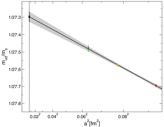
4.6 Results

The quark mass fits have fit qualities in the range $Q=0.05-0.99$, with an average fit quality of $Q=0.62$. The final results on the elements of the mixing matrix are given in Fig. S5. Evidently, the mixing matrix provides only a small correction to the leading order prediction of chiral perturbation theory, where the mixing matrix is the identity.

Figure S5: Final results for the elements of the Jacobian matrix (S20). There are only small corrections to the leading order $\chi$PT predictions.

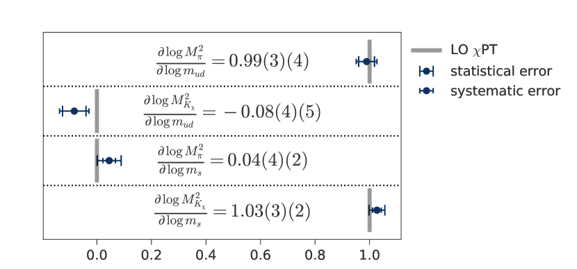
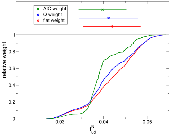
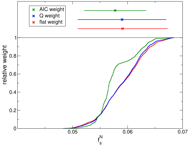
Applying the Jacobian matrix to the vector, $(F_{\pi^{+}}^{N},F_{K_{\chi}}^{N})^{T}$, we obtain the final results listed in Table 1. We use a weighted average and standard deviation of the results from the individual analyses to determine central value and systematic errors  (?, ?). For our main result, we use the Akaike information criterion (AIC)  (?) to determine the relative weight of the analyses. In order to check that the choice of weight does not significantly alter the result, we have plotted the cumulative distribution function of $f^{N}_{ud}$ and $f^{N}_{s}$ in Figs. S6 and S7, with a flat, unit weight, with a weight equal to the quality of fit, $Q$, and with the AIC weight. The choice of weight does not substantially influence the final result.

Figure S6: The cumulative distribution function of $f^{N}_{ud}$ over all analyses, obtained using three different weight functions. In the top part of the figure, the resulting central values and total errors, corresponding to each weight function, are plotted.

Figure S7: The cumulative distribution function of $f^{N}_{s}$ over all analyses, obtained using three different weight functions. In the top part of the figure, the resulting central values and total errors, corresponding to each weight function, are plotted.

Our results are largely compatible with other recent lattice determinations  (?, ?, ?, ?, ?, ?) as well as with the seminal calculations by Gasser, Leutwyler and Sainio  (?), while recent phenomenological determinations that obtain $f^{N}_{ud}$ from $\pi N$ scattering data  (?, ?, ?, ?, ?) give somewhat higher values.

5 Heavy quark effective theory

Scalar quark contents, the nucleon mass and the QCD trace anomaly are related by a sum rule  (?). This sum rule allows one to compute the heavy-quark contents from the light-quark ones, in the heavy-quark limit. This is achieved by considering a succession of effective field theories of QCD in which the heavy top, bottom and charm quarks are integrated out in turn. Thus, consider QCD with $N_{f}$ flavors treated as light and with one heavy quark, $Q$, to be integrated out. Then, matching the $N_{f}+1$ and $N_{f}$ theories at scale $m_{Q}$ yields (?) yields

$$f^{N}_{Q}=\frac{2}{3\beta_{0}}(1-\bar{f}_{N_{f}})\left[1+O\left(\left(\frac{\Lambda_{QCD}}{m_{Q}}\right)^{2},\alpha_{s}(m_{Q})\right)\right]$$ (S33)

where $\beta_{0}=11-(2/3)N_{f}$ is the leading-order coefficient of the QCD $\beta$-function, in $N_{f}$-flavor QCD, and

$$\bar{f}_{N_{f}}=\sum_{i=1}^{N_{f}}f^{N}_{q_{i}}$$ (S34)

is the sum of the scalar quark contents over the $N_{f}$ quark flavors, $q_{i}$, not integrated out. Recently, higher-order QCD corrections to (S33) have been computed to $O(\alpha_{s}^{3})$  (?), yielding

$$f_{Q}=\sum_{n=0}^{3}(b^{N_{f}}_{n}-c^{N_{f}}_{n}\bar{f}_{N_{f}})\alpha_{s}^{n}\left[1+O\left(\left(\frac{\Lambda_{QCD}}{m_{Q}}\right)^{2},\alpha_{s}^{4}(m_{Q})\right)\right])$$ (S35)

where $N_{f}=5$ for $Q=t$, $N_{f}=4$ for $Q=b$ and $N_{f}=3$ for $Q=c$. The numerical values of the $b_{n}$ and $c_{n}$ are given in Table S6 for $N_{f}=3,4$ and $5$.

$n$	$b_{n}^{3}$	$c_{n}^{3}$	$b_{n}^{4}$	$c_{n}^{4}$	$b_{n}^{5}$	$c_{n}^{5}$
0	0.0740741	0.0740741	0.08	0.08	0.0869565	0.0869565
1	0.0229236	0.0700806	0.0308124	0.081742	0.0412178	0.0965761
2	0.0412178	0.0534895	0.0157223	0.0664099	0.0246729	0.0846867
3	-0.012595	-0.0245554	-0.0218678	-0.0409409	-0.0334609	-0.0578502

Table S6: Coefficients in the heavy quark expansion (S35) from  (?).

We leverage these results in various ways. First, we can obviously use our results for the light quark contents to determine various $\bar{f}_{N_{f}}$ and thus the heavy-quark contents. This method is used to compute $f^{N}_{b}$ and $f^{N}_{t}$ in Sec. 7.

Now, if only the top quark is integrated out, the neglected corrections in (S35) are neglible. If also the bottom quark is removed from the dynamics, these corrections are still very small since $(\Lambda_{QCD}/m_{b})^{2}\sim 0.6\%$ ($\alpha_{s}(m_{b})^{4}$ is smaller). The heavy-quark expansion is possibly less-well behaved for the charm. Indeed, $(\Lambda_{QCD}/m_{c})^{2}\sim 6\%$ ($\alpha_{s}(m_{c})^{4}{\ \lower-1.2pt\vbox{\hbox{\hbox to0.0pt{$<$\hss}\lower 5.0pt\vbox{\hbox{$\sim$}}}}\ }2\%$ is smaller), which is no longer negligible and is comparable to our lattice uncertainties. Thus, we also compute $f^{N}_{c}$ directly on the lattice, using the Feynman-Hellmann theorem. As shown in Sec. 6, the result obtained is compatible with the one given by the heavy-quark expansion, within the naive estimate of $O((\Lambda_{QCD}/m_{c})^{2})$ corrections. This indicates that, even for the charm, the heavy-quark expansion behaves as expected.

The heavy-quark expansion also helps in the direct determination of the scalar, charm-quark content on the lattice. Since the nucleon mass depends on the charm-quark mass only very mildly, we vary this mass by $\pm 25\%$ around its physical value and measure the corresponding variations of the nucleon mass:

$$\begin{matrix}\Delta_{+}&=&M_{N}(m_{c}=\frac{5}{4}m_{c}^{\phi})-M_{N}(m_{c}=m_{c}^{\phi})\ ,\\ \Delta_{-}&=&M_{N}(m_{c}=m_{c}^{\phi})-M_{N}(m_{c}=\frac{3}{4}m_{c}^{\phi})\ .\end{matrix}$$ (S36)

These are then combined to determine the quantity

$$\hat{f}^{N}_{c}=2\frac{\Delta_{+}+\Delta_{-}}{M_{N}(m_{c}=m_{c}^{\phi})}$$ (S37)

which, using a second order Taylor series expansion in $m_{c}$ around the physical point, can be shown to equal the scalar, charm-quark content $f^{N}_{c}$, up to terms of order $(\delta m_{c}/m_{c})^{2}=1/16$.

Insight from the heavy-quark expansion provides an alternative expansion. First we note that $\alpha_{s}$ changes roughly between $0.5$ and $0.34$ when changing the scale from $3/4m_{c}^{\phi}$ to $5/4m_{c}^{\phi}$  (?), implying a relative variation of $f^{N}_{c}$ in this range by $\sim 3\%$ according to (S35). To a good approximation $f^{N}_{c}(m_{c})$, in this range, is therefore constant, i.e.

$$f^{N}_{c}(km_{c})=\left.\frac{\partial}{\partial\ln m}\ln M(m)\right|_{m=km_{c}}\simeq\text{cst}$$ (S38)

for $k=0.75$ or $k=1.25$. This implies

$$M(m_{c})=M(m_{c}^{\phi})\left(\frac{m_{c}}{m_{c}^{\phi}}\right)^{f^{N}_{c}}\ .$$ (S39)

Taylor expanding this expression to second order around $f_{c}=0$ and plugging the result into (S36), we find that the quantity,

$$\tilde{f}^{N}_{c}=\frac{1}{M(m_{c}^{\phi})\ln\frac{5}{4}\ln\frac{4}{3}\ln\frac{5}{3}}\left(\left(\ln\frac{4}{3}\right)^{2}\Delta_{+}+\left(\ln\frac{5}{4}\right)^{2}\Delta_{-}\right)\ ,$$ (S40)

is equal to the charm-quark content $f^{N}_{c}$, up to terms of order $(f^{N}_{c})^{3}\sim 3\times 10^{-4}$, assuming $f^{N}_{c}$ to be constant in the $\pm 25\%$ region around the physical charm quark mass. Since the heavy-quark expansion tells us that this assumption is valid to $O(3\%)$, we conclude that $\tilde{f}^{N}_{c}=f^{N}_{c}+O(3\%)$. The difference between $\hat{f}^{N}_{c}$ extracted with the Taylor series (S37) and $\tilde{f}^{N}_{c}$ extracted with the heavy quark expansion (S40) provides an estimate of the systematic error due to replacing the derivative of the nucleon mass, with respect to $m_{c}$, by a finite difference.

6 Lattice computation of the $c$ sigma term

The direct computation of the charm-quark content from our lattice ensembles poses a different set of challenges. On the one hand, locating the physical point precisely is not critical, as detailed in the previous section. On the other hand, one needs to vary the charm-quark mass over a significant range to obtain a signal. The strategy that we employ takes these two considerations into account. Instead of performing a combined fit to the dependence of the nucleon mass on lattice spacing, quark masses and volume and using the result to compute its derivative with respect to $m_{c}$, we directly determing the charm-quark content from finite differences (S37,S40) at each lattice spacing. The central ensembles, at each lattice spacing, are tuned to the physical mass point to within less than 4 % in the light and strange quark masses leading to tiny corrections covered by the variation of finite-difference forms (S37,S40). Furthermore, since the ensembles at one lattice spacing share all parameters except for the charm-quark mass, and $M_{\pi}L>4$, finite-volume effects are irrelevant too.

6.1 Analysis details

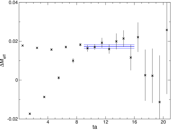
We compute the mass differences $\Delta_{\pm}$ of (S36) directly from the ratio of nucleon correlators from the two relevant ensembles. Staggered excited states in the two nucleon correlators are suppressed by using the time-shifted propagator described in Sec. 2.4, for each of the ensembles separately. Fig. S8 shows an effective mass plateau for $\Delta_{M}=\Delta_{+}+\Delta_{-}$, for our $\beta=3.84$ ensembles. We identify the onset of the plateau to be slightly below $t_{\mathrm{min}}\sim 0.8\,\mathrm{fm}$ and correspondingly consider two values, $t_{\mathrm{min}}\simeq 0.8\,\mathrm{fm}$ and $t_{\mathrm{min}}\simeq 0.95\,\mathrm{fm}$, for determining the mass difference. The variation of the result with respect to $t_{\mathrm{min}}$ enters into the systematic error.

Figure S8: Effective mass plateau and extracted mass from the more aggressive fit with $t_{\mathrm{min}}\sim 0.8\,\mathrm{fm}$ at $\beta=3.84$.

We determine the lattice spacing either by interpolating the pseudoscalar decay constant $f_{\pi}$ as describes in Sec. 4.3 or by directly using the nucleon mass from the central, physical ensemble at each $\beta$. The difference between these two procedures also enters into the systematic error estimate.

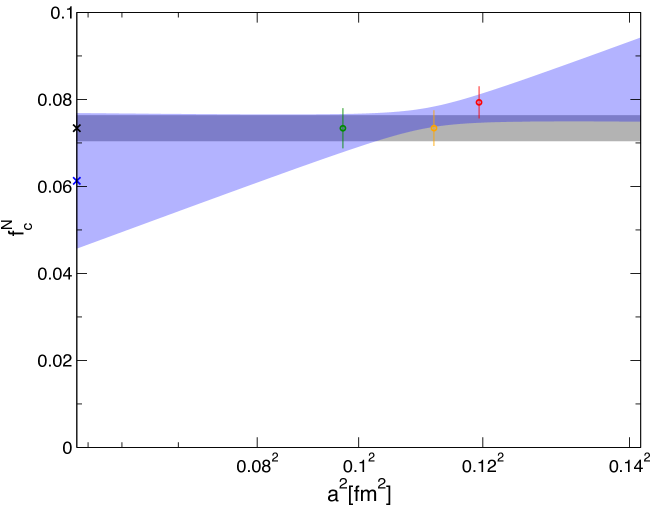
In order to estimate cutoff uncertainties, we perform three different continuum extrapolations of $f^{N}_{c}$. Using values from all three lattice spacings, we perform either a constant or linear extrapolation in $a^{2}$. In addition, we also perform a constant extrapolation using the two finest lattice spacings only. The result from two of these extrapolations is plotted in fig. S9. The spread between the results of these methods again enters the systematic error.

Figure S9: Continuum extrapolation of the scalar, charm-quark content of the nucleon, $f^{N}_{c}$. The blue curve and point correspond to a linear extrapolation in $a^{2}$ using all three lattice spacings while the grey curve and black point corresponds to a constant extrapolation to the results from our two finest lattices.

6.2 Systematic error variations

We perform a total of 2($\hat{f}^{N}_{c}$,$\tilde{f}^{N}_{c}$)$\times$2(fit range) $\times$2(Scale setting)$\times$3(continuum extrapolation)$=24$ different analysis procedures. The way in which we combine these analyses to give a final central value and systematic error is described in Sec. 6.4.

Figure S10: Variation of $f_{c}^{N}$ from different restrictions to the full analysis procedure. From top to bottom these are: restriction to a single plateau range, to a single scaling behavior, to a single definition for $f^{N}_{c}$ and to a single scale-setting method. The last row shows the final result including all fits. The average fit quality of the analyses $\bar{Q}$ is given in each case. The percentage of the total systematic error due to each variation alone is also displayed (percentages add up in quadrature).

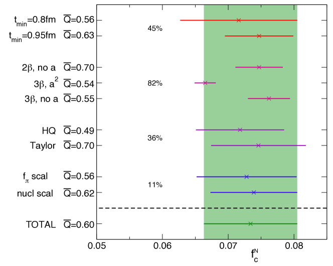
Fig. S10 gives a breakup of the systematic error into its different components. As one can see, all restrictions of the fit procedure are in agreement with the final result and the main contribution to the systematic uncertainty originates from varying the continuum fit.

6.3 Crosschecks

As discussed in Sec. 6, heavy-quark effective theory provides us with a crosscheck of the charm sigma term up to a precision of $O((\Lambda_{QCD}/m_{c})^{2})\sim 6\%$. We enter, into the heavy-quark expansion (S35), $\alpha_{s}(m_{c})=0.388(13)$ originating from $m_{c}(m_{c})=1.275({+25\atop-35})\mathrm{GeV}$  (?) and the numerically integrated 5-loop beta function  (?) with $\alpha_{s}(91.187\mathrm{GeV})=0.1181$  (?). This results in

$$f_{c}^{N}|_{\text{HQ}}=0.08374(34)-0.1078(14)\bar{f}_{3}$$ (S41)

where $\bar{f}_{3}$ denotes the sum of quark contents of the lighter quarks

$$\bar{f}_{3}=\sum_{q=ud,s}f_{q}^{N}\ .$$ (S42)

Our light quark results give

$$\bar{f}_{3}=0.0975(56)(52)\ ,$$ (S43)

yielding

$$f_{c}^{N}|_{\text{HQ}}=0.07323(61)(65)$$ (S44)

This result is in excellent agreement with the one from the direct lattice determination.

6.4 Results

The continuum extrapolations have fit qualities in the range $Q=0.25-1.00$, with an average fit quality $\bar{Q}=0.60$.

Figure S11: The cumulative distribution function of $f^{N}_{c}$ over all analyses, obtained using three different weight functions. In the top part of the figure, the resulting central values and total errors, corresponding to each weight function, are plotted.

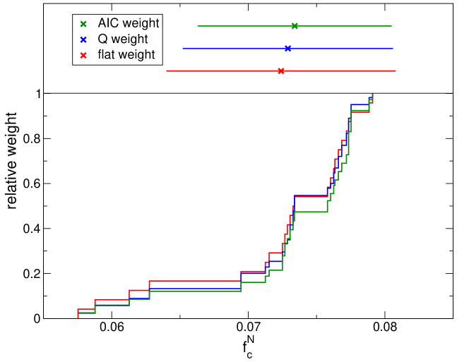
As in the case of the light and strange quark contents, we plot the cumulative distribution function of $f^{N}_{c}$ from all analyses with different weight functions (see Fig. S11). The choice of the weighting function does not significantly affect our result and we take the AIC weight for producing our final result.

The lattice calculation of $f^{N}_{c}$  (?, ?, ?) is compatible with our number. So is the determination of  (?), in which systematic errors are not estimated.

7 Heavy-quark expansion for the $b$, and $t$ $\sigma$-terms

Having checked the validity of the heavy-quark expansion (S35) in the case of the charm, we use it to compute $f^{N}_{b}$ and $f^{N}_{t}$. We use as inputs $\alpha_{s}(m_{b/t})=0.225(3)/0.109(1)$ originating from $m_{b}(m_{b})=4.18({+4\atop-3})\mathrm{GeV}$ and $m_{t}(m_{t})=160.0({+4.8\atop-4.3})\mathrm{GeV}$  (?) and the numerically integrated 5-loop beta function  (?) with $\alpha_{s}(91.187\mathrm{GeV})=0.1181$  (?). Then, expression (S35) for $f^{N}_{b}$ and $f^{N}_{t}$ becomes:

$$\begin{matrix}f_{b}^{N}&=&0.08748(13)-0.10129(39)\bar{f}_{4}\ ,\\ f_{t}^{N}&=&0.09169(4)-0.09840(10)\bar{f}_{5}\end{matrix}$$ (S45)

where $\bar{f}_{N_{f}}$ denotes the sum of scalar, quark contents defined in (S34).

We input our lattice results into these equations to obtain the final numbers reported in Table 1. The statistical error originates from the lattice input while systematic error estimates from the heavy-quark expansion $(\Lambda_{QCD}/m_{b})^{2}=0.6\%$, from the lattice and from $\alpha_{s}$ are combined in quadrature to give the systematic error. The errors on $f_{b}^{N}$ and $f_{t}^{N}$ are both dominated entirely by lattice errors on the light, strange and charm quark contents used as input quantities.

8 Arbitrary linear combinations of $\sigma$-terms with full correlations

We provide a C routine that computes arbitrary linear combinations of the scalar, quark contents for the proton, the neutron and the nucleon, while retaining the full correlation between those quantities. When called without arguments, it returns the individual quark contents as well as the Higgs-nucleon coupling, $f^{N}_{h}$, and brief instructions on how to obtain any other linear combination.

The code is available as an ancillary file or via download from http://particle.uni-wuppertal.de/hch/lincomb.c

References

- 1. Marc Schumann “Direct Detection of WIMP Dark Matter: Concepts and Status” In J. Phys. G46.10, 2019, pp. 103003 DOI: 10.1088/1361-6471/ab2ea5
- 2. Satoshi Mihara “COMET/Mu2e/MEG” In 16th Conference on Flavor Physics and CP Violation 234, 2019, pp. 149–156 DOI: 10.1007/978-3-030-29622-3_21
- 3. Kenneth G. Wilson “Confinement of Quarks” [,45(1974)] In Phys. Rev. D10, 1974, pp. 2445–2459 DOI: 10.1103/PhysRevD.10.2445
- 4. S. Duane, A.. Kennedy, B.. Pendleton and D. Roweth “Hybrid Monte Carlo” In Phys. Lett. B195, 1987, pp. 216–222 DOI: 10.1016/0370-2693(87)91197-X
- 5. Mikhail A. Shifman, A.. Vainshtein and Valentin I. Zakharov “Remarks on Higgs Boson Interactions with Nucleons” In Phys. Lett. B78, 1978, pp. 443–446 DOI: 10.1016/0370-2693(78)90481-1
- 6. Please see Supplementary Online Material
- 7. Steven Weinberg “Pion scattering lengths” In Phys. Rev. Lett. 17, 1966, pp. 616–621 DOI: 10.1103/PhysRevLett.17.616
- 8. J. Gasser, H. Leutwyler and M.. Sainio “Sigma term update” In Phys. Lett. B253, 1991, pp. 252–259 DOI: 10.1016/0370-2693(91)91393-a
- 9. M.. Pavan, I.. Strakovsky, R.. Workman and R.. Arndt “The Pion nucleon Sigma term is definitely large: Results from a G.W.U. analysis of pi nucleon scattering data” In Meson nucleon physics and the structure of the nucleon. Proceedings, 9th International Symposium, MENU 2001, Washington, USA, July 26-31, 2001 16, 2002, pp. 110–115 arXiv:hep-ph/0111066 [hep-ph]
- 10. Martin Hoferichter, J. Ruiz de Elvira, Bastian Kubis and Ulf-G. Meißner “High-Precision Determination of the Pion-Nucleon Term from Roy-Steiner Equations” In Phys. Rev. Lett. 115.9, 2015, pp. 092301 DOI: 10.1103/PhysRevLett.115.092301
- 11. R. Horsley et al. “Hyperon sigma terms for 2+1 quark flavours” In Phys. Rev. D85, 2012, pp. 034506 DOI: 10.1103/PhysRevD.85.034506
- 12. S. Durr et al. “Lattice computation of the nucleon scalar quark contents at the physical point” In Phys. Rev. Lett. 116.17, 2015, pp. 172001 DOI: 10.1103/PhysRevLett.116.172001
- 13. Gunnar S. Bali et al. “Direct determinations of the nucleon and pion terms at nearly physical quark masses” In Phys. Rev. D93.9, 2016, pp. 094504 DOI: 10.1103/PhysRevD.93.094504
- 14. Yi-Bo Yang et al. “N and strangeness sigma terms at the physical point with chiral fermions” In Phys. Rev. D94.5, 2016, pp. 054503 DOI: 10.1103/PhysRevD.94.054503
- 15. A. Abdel-Rehim et al. “Direct Evaluation of the Quark Content of Nucleons from Lattice QCD at the Physical Point” In Phys. Rev. Lett. 116.25, 2016, pp. 252001 DOI: 10.1103/PhysRevLett.116.252001
- 16. C. Alexandrou et al. “The nucleon axial, tensor and scalar charges and -terms in lattice QCD” 1909.00485, 2019 arXiv:1909.00485 [hep-lat]
- 17. H. Ohki et al. “Nucleon strange quark content from lattice QCD with exact chiral symmetry” In Phys. Rev. D87, 2013, pp. 034509 DOI: 10.1103/PhysRevD.87.034509
- 18. Walter Freeman and Doug Toussaint “Intrinsic strangeness and charm of the nucleon using improved staggered fermions” In Phys. Rev. D88, 2013, pp. 054503 DOI: 10.1103/PhysRevD.88.054503
- 19. Parikshit Junnarkar and Andre Walker-Loud “Scalar strange content of the nucleon from lattice QCD” In Phys. Rev. D87, 2013, pp. 114510 DOI: 10.1103/PhysRevD.87.114510
- 20. M. Gong “Strangeness and charmness content of the nucleon from overlap fermions on 2+1-flavor domain-wall fermion configurations” In Phys. Rev. D88, 2013, pp. 014503 DOI: 10.1103/PhysRevD.88.014503
- 21. C. Patrignani “Review of Particle Physics” In Chin. Phys. C40.10, 2016, pp. 100001 DOI: 10.1088/1674-1137/40/10/100001
- 22. S. Aoki “Review of lattice results concerning low-energy particle physics” In Eur. Phys. J. C77.2, 2017, pp. 112 DOI: 10.1140/epjc/s10052-016-4509-7
- 23. S. Dürr “Ab Initio Determination of Light Hadron Masses” In Science 322, 2008, pp. 1224–1227 DOI: 10.1126/science.1163233
- 24. Sz. Borsanyi “Ab initio calculation of the neutron-proton mass difference” In Science 347, 2015, pp. 1452–1455 DOI: 10.1126/science.1257050
- 25. Richard J. Hill and Mikhail P. Solon “Standard Model anatomy of WIMP dark matter direct detection II: QCD analysis and hadronic matrix elements” In Phys. Rev. D91, 2015, pp. 043505 DOI: 10.1103/PhysRevD.91.043505
- 26. Martin Hoferichter, Philipp Klos, Javier Menéndez and Achim Schwenk “Improved limits for Higgs-portal dark matter from LHC searches” In Phys. Rev. Lett. 119.18, 2017, pp. 181803 DOI: 10.1103/PhysRevLett.119.181803
- 27. K. Kajantie, M. Laine, K. Rummukainen and Mikhail E. Shaposhnikov “Is there a hot electroweak phase transition at m(H) larger or equal to m(W)?” In Phys. Rev. Lett. 77, 1996, pp. 2887–2890 DOI: 10.1103/PhysRevLett.77.2887
- 28. F. Csikor, Z. Fodor and J. Heitger “Endpoint of the hot electroweak phase transition” In Phys. Rev. Lett. 82, 1999, pp. 21–24 DOI: 10.1103/PhysRevLett.82.21
- 29. Y. Aoki et al. “The Order of the quantum chromodynamics transition predicted by the standard model of particle physics” In Nature 443, 2006, pp. 675–678 DOI: 10.1038/nature05120
- 30. P. Güttinger “Das Verhalten von Atomen im magnetischen Drehfeld” In Zeitschrift für Physik 73.3, 1932, pp. 169–184 DOI: 10.1007/BF01351211
- 31. Wolfgang Pauli “Principles of Wave Mechanics” In Handbuch der Physik, vol. 24 Berlin: Springer, 1933, pp. 162
- 32. H. Hellmann “Zur Rolle der kinetischen Elektronenenergie für die zwischenatomaren Kräfte” In Zeitschrift für Physik 85.3, 1933, pp. 180–190 DOI: 10.1007/BF01342053
- 33. R.. Feynman “Forces in Molecules” In Phys. Rev. 56, 1939, pp. 340–343 DOI: 10.1103/PhysRev.56.340
- 34. Xiang-Dong Ji “Breakup of hadron masses and energy - momentum tensor of QCD” In Phys. Rev. D52, 1995, pp. 271–281 DOI: 10.1103/PhysRevD.52.271
- 35. “Combined measurements of Higgs boson production and decay using up to 80 fb-1 of proton–proton collision data at 13 TeV collected with the ATLAS experiment”, 2018 URL: https://cds.cern.ch/record/2629412
- 36. Xiang-Dong Ji “A QCD analysis of the mass structure of the nucleon” In Phys. Rev. Lett. 74, 1995, pp. 1071–1074 DOI: 10.1103/PhysRevLett.74.1071
- 37. Yi-Bo Yang et al. “Proton Mass Decomposition from the QCD Energy Momentum Tensor”, 2018 arXiv:1808.08677 [hep-lat]
- 38. Gilberto Colangelo, Stephan Durr and Christoph Haefeli “Finite volume effects for meson masses and decay constants” In Nucl. Phys. B721, 2005, pp. 136–174 DOI: 10.1016/j.nuclphysb.2005.05.015
- 39. Szabocls Borsanyi et al. “Full result for the QCD equation of state with 2+1 flavors” In Phys. Lett. B730, 2014, pp. 99–104 DOI: 10.1016/j.physletb.2014.01.007
- 40. R. Bellwied et al. “Fluctuations and correlations in high temperature QCD” In Phys. Rev. D92.11, 2015, pp. 114505 DOI: 10.1103/PhysRevD.92.114505
- 41. C… Davies et al. “Precise Charm to Strange Mass Ratio and Light Quark Masses from Full Lattice QCD” In Phys.Rev.Lett.104:132003,2010 104, 2010, pp. 132003 DOI: 10.1103/PhysRevLett.104.132003
- 42. MILC “MILC code Version 7”, 2013 URL: http://www.physics.utah.edu/~detar/milc/milc_qcd.html
- 43. Gilberto Colangelo, Andreas Fuhrer and Stefan Lanz “Finite volume effects for nucleon and heavy meson masses” In Phys. Rev. D82, 2010, pp. 034506 DOI: 10.1103/PhysRevD.82.034506
- 44. M. Tanabashi “Review of Particle Physics” In Phys. Rev. D98.3, 2018, pp. 030001 DOI: 10.1103/PhysRevD.98.030001
- 45. A. Bazavov “Charmed and light pseudoscalar meson decay constants from four-flavor lattice QCD with physical light quarks” In Phys. Rev. D90.7, 2014, pp. 074509 DOI: 10.1103/PhysRevD.90.074509
- 46. S. Durr et al. “Lattice QCD at the physical point: light quark masses” In Phys. Lett. B701, 2011, pp. 265–268 DOI: 10.1016/j.physletb.2011.05.053
- 47. H. Akaike In IEEE Transactions on Automatic Control 19, 1974, pp. 716
- 48. Constantia Alexandrou and Christos Kallidonis “Low-lying baryon masses using twisted mass clover-improved fermions directly at the physical pion mass” In Phys. Rev. D96.3, 2017, pp. 034511 DOI: 10.1103/PhysRevD.96.034511
- 49. C. Alexandrou “Nucleon scalar and tensor charges using lattice QCD simulations at the physical value of the pion mass” [erratum: Phys. Rev.D96,no.9,099906(2017)] In Phys. Rev. D95.11, 2017, pp. 114514 DOI: 10.1103/PhysRevD.96.099906 SMASH, 10.1103/PhysRevD.95.114514
- 50. Xiu-Lei Ren, Xi-Zhe Ling and Li-Sheng Geng “Pionnucleon sigma term revisited in covariant baryon chiral perturbation theory” In Phys. Lett. B783, 2018, pp. 7–12 DOI: 10.1016/j.physletb.2018.05.063
- 51. J.. Alarcon, J. Martin Camalich and J.. Oller “The chiral representation of the scattering amplitude and the pion-nucleon sigma term” In Phys. Rev. D85, 2012, pp. 051503 DOI: 10.1103/PhysRevD.85.051503
- 52. Yun-Hua Chen, De-Liang Yao and H.. Zheng “Analyses of pion-nucleon elastic scattering amplitudes up to in extended-on-mass-shell subtraction scheme” In Phys. Rev. D87, 2013, pp. 054019 DOI: 10.1103/PhysRevD.87.054019
- 53. Martin Hoferichter, Jacobo Ruiz de Elvira, Bastian Kubis and Ulf-G. Meißner “Roy-Steiner-equation analysis of pion-nucleon scattering” In Phys. Rept. 625, 2016, pp. 1–88 DOI: 10.1016/j.physrep.2016.02.002
- 54. P.. Baikov, K.. Chetyrkin and J.. Kühn “Five-Loop Running of the QCD coupling constant” In Phys. Rev. Lett. 118.8, 2017, pp. 082002 DOI: 10.1103/PhysRevLett.118.082002