Graph Neural Networks with Continual Learning for Fake News Detection from Social Media
Abstract.
Although significant effort has been applied to fact-checking, the prevalence of fake news over social media, which has profound impact on justice, public trust and our society as a whole, remains a serious problem. In this work, we focus on propagation-based fake news detection, as recent studies have demonstrated that fake news and real news spread differently online. Specifically, considering the capability of graph neural networks (GNNs) in dealing with non-Euclidean data, we use GNNs to differentiate between the propagation patterns of fake and real news on social media. In particular, we concentrate on two questions: (1) Without relying on any text information, e.g., tweet content, replies and user descriptions, how accurately can GNNs identify fake news? Machine learning models are known to be vulnerable to adversarial attacks, and avoiding the dependence on text-based features can make the model less susceptible to the manipulation of advanced fake news fabricators. (2) How to deal with new, unseen data? In other words, how does a GNN trained on a given dataset perform on a new and potentially vastly different dataset? If it achieves unsatisfactory performance, how do we solve the problem without re-training the model on the entire data from scratch, which would become prohibitively expensive in practice as the data volumes grow? We study the above questions on two datasets with thousands of labelled news items, and our results show that: (1) GNNs can achieve comparable or superior performance without any text information to state-of-the-art methods. (2) GNNs trained on a given dataset may perform poorly on new, unseen data, and direct incremental training cannot solve the problem—this issue has not been addressed in the previous work that applies GNNs for fake news detection. In order to solve the problem, we propose a method that achieves balanced performance on both existing and new datasets, by using techniques from continual learning to train GNNs incrementally.
1. Introduction
While social media has facilitated the timely delivery of various types of information around the world, a consequence is that news is emerging at an unprecedented rate, making it increasingly difficult to fact-check. A series of incidents over recent years have demonstrated the significant damage fake news can cause to society. Therefore, how to automatically and accurately identify fake news before it is widespread has become an urgent challenge for research. Here we use the definition in (Zhou and Zafarani, 2018): fake news is intentionally and verifiably false news published by a news outlet—similar definitions have also been used in previous studies on fake news detection (Monti et al., 2019; Shu et al., 2019a, 2017; Ruchansky et al., 2017).
In our work, we focus on a propagation-based approach for fake news detection. In other words, we use the propagation pattern of news on social media, e.g., tweets and retweets of news on Twitter, to determine whether it is fake or not. The feasibility of this approach builds on (1) empirical evidence that fake news and real news spread differently online (Vosoughi et al., 2018); and (2) the latest development in graph neural networks (GNNs) (Bruna et al., 2013; Niepert et al., 2016; Ying et al., 2018; Wu et al., 2019) that has enhanced the performance of machine learning models on non-Euclidean data. In addition, as pointed out in (Monti et al., 2019), whereas content-based approaches require syntactic and semantic analyses, propagation-based approaches are language-agnostic, and can be less vulnerable to adversarial attacks (Szegedy et al., 2013; Goodfellow et al., 2014), where advanced news fabricators carefully manipulate the content in order to bypass detection.
The idea of using propagation patterns to detect fake news has been explored in a number of previous studies (Wu et al., 2015; Ma et al., 2017; Wu and Liu, 2018; Liu and Wu, 2018; Zhou and Zafarani, 2019; Shu et al., 2019b), where different types of models have been considered: Wu et al. (Wu et al., 2015) use a hybrid Support Vector Machine (SVM), Ma et al. (Ma et al., 2017) use Propagation Tree Kernel; Wu et al. (Wu and Liu, 2018) incorporate Long Short-Term Memory (LSTM) cells into the Recurrent Neural Network (RNN) model; Liu et al. (Liu and Wu, 2018) use both RNNs and Convolutional Neural Networks (CNNs); Shu et al. (Shu et al., 2019b) and Zhou et al. (Zhou and Zafarani, 2019) propose different types of features and compare multiple commonly used machine learning models. The most relevant works include (Monti et al., 2019; Lu and Li, 2020; Bian et al., 2020), which also apply GNNs to study propagation patterns. However, in addition to selecting a different GNN algorithm specifically designed for graph classification (refer to Section 2 for further explanation), our work mainly focuses on the following questions:
-
•
Question 1: Without relying on any text information, e.g., tweet content, replies and user descriptions, how accurately can GNNs identify fake news? It is demonstrated in Section 3 that even though our model is limited to a restricted set of non-textual features obtained from user profiles and timeline tweets, GNNs can be trained on propagation patterns and these features to achieve comparable or superior performance to state-of-the-art methods that require sophisticated analyses on tweet content, user replies, etc. We argue that the limited set of features can further enhance the security of our models against adversarial attacks, as previous work has shown that high dimensionality facilitates the generation of adversarial samples, resulting in an increased attack surface (Wang et al., 2016).
-
•
Question 2: How to deal with new, unseen data? The above question is only concerned with the performance of GNNs on a single dataset. However, a trained model may face vastly different data in practice, and it is important to further investigate how models perform in this scenario. Specifically, we find that GNNs trained on a given dataset may perform poorly on another dataset, and direct incremental training cannot solve the problem—this issue has not been discussed in the previous work that uses GNNs for fake news detection. In order to solve the problem, we propose a method that applies techniques from continual learning to train GNNs incrementally, so that they achieve balanced performance on both existing and new datasets. The method avoids re-training the model on the entire data from scratch—new data always exist, and this becomes prohibitively expensive as data volumes grow.
The remainder of this paper is organised as follows: Section 2 briefly introduces the background on graph neural networks; Section 3 describes our content-free, GNNs-based fake news detection algorithm; Section 4 investigates how to deal with new, unseen data, and proposes a solution to achieve balanced performance on both existing and new data by applying techniques from continual learning; Section 5 reviews previous work in fake news detection on social media; and finally Section 6 concludes the paper and offers directions for future work.
2. Background on Graph Neural Networks
Although deep learning has witnessed tremendous success in a wide range of applications, including image classification, natural language processing and speech recognition, it mostly deals with data in Euclidean space. GNNs (Bruna et al., 2013; Niepert et al., 2016; Ying et al., 2018; Wu et al., 2019), by contrast, are designed to process data generated from non-Euclidean domains.
Consider a graph with vertices/nodes and edges, where is the adjacency matrix. if there is an edge from node to node , and otherwise; is the feature matrix, i.e., each node has features. Given and as inputs, the output of a GNN, i.e., node embeddings, after the step is: , where is the propagation function parameterised by , and is initialised by the feature matrix, i.e., .
There have been a number of implementations for the propagation function. A simple form of the function is: , where is a non-linear activation function, e.g., the rectified linear unit (ReLU) function, and is the weight matrix for layer . A popular implementation of the function is (Kipf and Welling, 2017): , where , . Please refer to (Wu et al., 2019) for more choices of the function.
GNNs can perform node regression, node classification, link prediction, edge classification or graph classification depending on the requirements. In our work, since the goal is to label the propagation pattern of each item of news, which is a graph, we choose the algorithm of DiffPool (Ying et al., 2018) that is specifically designed for graph classification. DiffPool extends any existing GNN model by further considering the structural information of graphs. At each layer DiffPool takes the original output and the adjacency matrix , and learns a coarsened graph of nodes, with the adjacency matrix and the node embeddings .
3. Propagation-based Fake News Detection
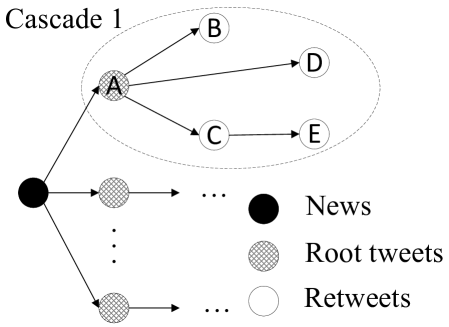
As mentioned in the introduction, we use the definition in (Zhou and Zafarani, 2018) that fake news is intentionally and verifiably false news published by a news outlet. Once an item of news is published, it may be tweeted by multiple users. We call these tweets that directly reference the news URL root tweets. Each of them and their retweets form a separate cascade (Vosoughi et al., 2018), and all the cascades form the propagation pattern of an item of news. The purpose of this work is to determine the validity of an item of news using its propagation pattern.
Formally, we define the propagation-based fake news detection problem as follows: given a set of labeled graphs , where is the propagation pattern for news , and is the label of graph , the goal is to learn a mapping that labels each graph.
In the remainder of this section, we first explain how we generate a graph in Section 3.1, i.e., the adjacency matrix and the feature matrix, and present the experimental results to verify the effectiveness of the GNN-based detection algorithm in Section 3.2.
3.1. Data Generation
In order to generate the news propagation pattern, we use the dataset of FakeNewsNet (Shu et al., 2018), which is especially collected for the purpose of fake news detection. FakeNewsNet contains labelled news from two websites: politifact.com111https://www.politifact.com/ and gossipcop.com222https://www.gossipcop.com/—the news content includes both linguistic and visual information, all the tweets and retweets for each item of news, and the information of the corresponding Twitter users (refer to (Shu et al., 2018) for more details).
Adjacency matrix. As illustrated in Fig. 1, each item of news is represented as a graph, where a node refers to a tweet (including the corresponding user)—either the root tweet that references the news or its retweets. A special case is that an extra node representing the news is added to connect all cascades together. All the feature values for this node are set to zero. Edges here represent information flow, i.e., how the news transfers from one person to another. However, Twitter APIs do not provide the immediate source of a retweet, e.g., in Cascade 1 of Fig. 1, Twitter APIs only show that and are retweets of , but is actually a retweet of . To solve this problem, within each cascade we first sort the tweets by their timestamps, and then search for the source of a retweet from all the tweets that are published earlier. Specifically, there is an edge from node to node 333Node is published before node , and the information goes from user to user . if:
-
•
The user of node mentions the user of node in the tweet, e.g., user retweets a news item and also recommends it to user via mentioning;
-
•
Tweet is public and tweet is posted within a certain period of time after tweet . We have tested different time limits from one hour to ten hours.
Note that edges only exist between nodes within the same cascade. We have also compared the difference by further considering the follower and following relations, but our results demonstrate that there is no significant improvement. In addition, since Twitter applies a much stricter rate limit on corresponding APIs, these types of information may not be available in real time, especially if a number of news items need to be validated at the same time and within a detection deadline. More details on this are given in the next subsection.
Feature matrix. As mentioned earlier we do not rely on any textual information in this work, including tweet content, user reply or user description, and only choose the following information from user profiles as the features for each node:
-
•
Whether the user is verified;
-
•
The timestamp when the user was created, encoded as the number of months since March 2006—the time when Twitter was founded;
-
•
The number of followers;
-
•
The number of friends;
-
•
The number of lists;
-
•
The number of favourites;
-
•
The number of statuses;
-
•
The timestamp of the tweet, encoded as the number of seconds since the first tweet references the news is posted.
Another important reason why we choose the above features is that they are most accessible—they are directly available within the tweet object, which is preferable for online detection.
In addition, based on the hypothesis that less credible users are more likely to form larger clusters than more credible users (Shu et al., 2020), we extract another set of features from user timeline tweets to check if they can further improve the performance of our model. Specifically, we collect the timeline tweets for all the users in the propagation pattern of a news item (a maximum of 200 tweets are collected per user), and construct another graph, where each node represents a user, while an edge exists from node to node if user mentions user , and the weight of the edge is the number of times that user is mentioned by user . Finally, after the graph is built we calculate the following features for each node :
-
•
The in-degree, i.e., the number of users that have mentioned user ;
-
•
The out-degree, i.e., the number of users that have been mentioned by user
-
•
The weighted in-degree, i.e., the number of times that user have been mentioned;
-
•
The weighted out-degree, i.e., the number of times that user have mentioned others;
-
•
The number of hop-2 in-neighbours;
-
•
The number of hop-2 out-neighbours;
-
•
The number of collected timeline tweets.
The rationale of studying these features is that less credible users are more likely to collaborate with each other, and such behaviour can be captured by the above features.
In our experiment, we first train models only using the features from user profiles, and then compare the difference with (1) training models on the features from timeline tweets, and (2) training models on a combination of both sets of features.
3.2. Experimental Verification
Using the method introduced in the previous subsection to generate the graphs (the adjacency and feature matrices), we test multiple DiffPool models with a range of different architectures: 2-4 pooling layers, 16-128 hidden dimensions and 16-128 embedding dimensions (the chosen hyper-parameters under different settings are given later in this section). As recommended by the authors in (Ying et al., 2018), we use DiffPool built on top of GraphSage (Hamilton et al., 2017).
In order to make our results comparable with those reported in (Shu et al., 2019a) (as they also tested fake news detection algorithms on the same dataset), we follow the same procedure to train and test the GNNs: randomly choose 75% of the news as the training data while keeping the rest as the test data, and the final result is the average performance over five repeats. In addition, the model is evaluated with the following commonly used metrics: accuracy, precision, recall and F1 score. The main reason why we do not use the same split of training and test data across all experiments is that an algorithm may perform extremely well on one split of data but rather poorly on another. Therefore, all algorithms are tested on multiple random splits of data, so that the obtained results are closer to their real performance.
| Dataset | Metric | User profile features only | Timeline tweets features only | Combined | |||
|---|---|---|---|---|---|---|---|
| Without follower/ | With follower/ | Without follower/ | With follower/ | Without follower/ | With follower/ | ||
| following | following | following | following | following | following | ||
| PolitiFact | Acc | 0.811 | 0.805 | 0.699 | 0.696 | 0.792 | 0.803 |
| Pre | 0.809 | 0.806 | 0.700 | 0.694 | 0.792 | 0.806 | |
| Rec | 0.809 | 0.801 | 0.695 | 0.695 | 0.792 | 0.801 | |
| F1 | 0.808 | 0.801 | 0.693 | 0.691 | 0.791 | 0.801 | |
| GossipCop | Acc | 0.844 | 0.841 | 0.853 | 0.853 | 0.849 | 0.841 |
| Pre | 0.823 | 0.821 | 0.834 | 0.831 | 0.829 | 0.820 | |
| Rec | 0.833 | 0.834 | 0.852 | 0.846 | 0.840 | 0.831 | |
| F1 | 0.827 | 0.826 | 0.841 | 0.837 | 0.833 | 0.825 | |
3.2.1. Training on the Complete Dataset
We first train GNNs on the whole dataset of PolitiFact/GossipCop, using the features from user profile only, and without considering the follower/following relation. After testing a range of hyper-parameters, we find that a four-layer GNN with 64 hidden dimensions and 64 embedding dimensions works best for the dataset of PolitiFact, while for GossipCop the number of layers should decrease to two as there are significantly more news items in this dataset.
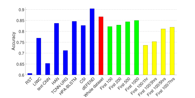
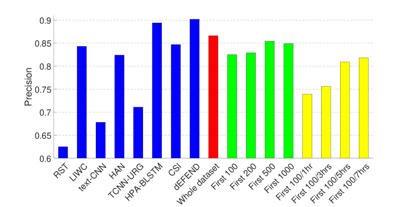
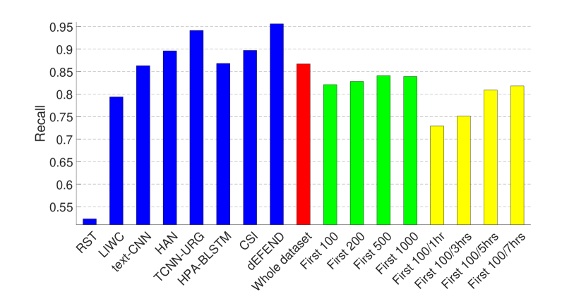
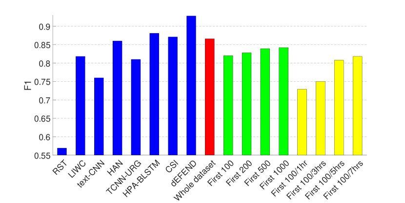
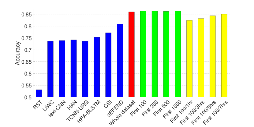
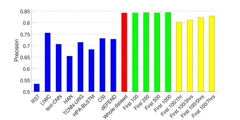
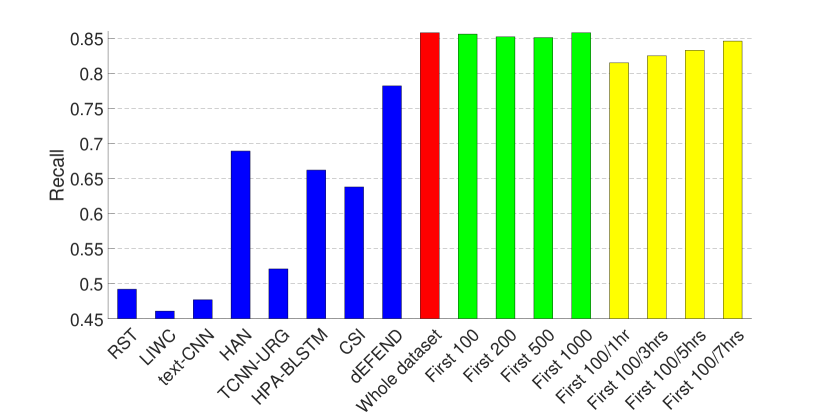
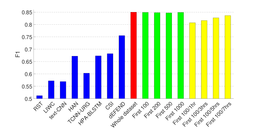
The experimental results are presented in Figs. 2 and 3, where (1) The first eight bars correspond to the results of eight fake news detection algorithms as reported in (Shu et al., 2019a) on the same dataset—RST (Rubin et al., 2015), LIWC (Pennebaker et al., 2015), HAN (Yang et al., 2016), text-CNN (Kim, 2014), TCNN-URG (Qian et al., 2018), HPA-BLSTM (Guo et al., 2018), CSI (Ruchansky et al., 2017) and dEFEND (Shu et al., 2019a). Note that all of these methods require analysis on textual information, e.g., tweet content and user replies. (2) The ninth bar in red is the result of our propagation-based method trained on the whole dataset.
As can be seen from the figures, by only relying on the limited set of non-textual features as introduced in Section 3.1, our model can achieve comparable performance on the dataset of PolitiFact, and the best result on the dataset of GossipCop.
3.2.2. Training on the Partial Dataset for Early Detection
It is critical to detect fake news at an early stage before it becomes widespread, since the wider fake news spreads, the more likely people would trust it (Boehm, 1994), and it is difficult to correct people’s perception towards an issue, even if the previous impression is inaccurate (keersmaecker and Roets, 2017).
Therefore, we train GNNs on the clipped dataset that contains for each news item (1) the first 100, 200, 500, 1000 tweets (green bars in Figs. 2 and 3); and (2) the first 100 tweets or tweets from the first one, three, five or seven hours, whichever is smaller (yellow bars in Figs. 2 and 3). The hyper-parameters here are the same as in the last set of experiments, except that for the clipped GossipCop dataset that contains the first 100 tweets (both with and without the different time limits), the number of pooling layers is three.
The results demonstrate that even with a limited number of tweets per news item, our model can achieve a decent performance, especially on the dataset of GossipCop, which is likely to be due to the larger size of the dataset.
3.2.3. Additional Non-textual Features from User Timeline Tweets
Here we investigate the impact of the set of non-textual features extracted from user timeline tweets as introduced in Section 3.1.
Note that from here forward we focus on models trained on the clipped dataset with the first 100 tweets or the tweets from the first five hours for each item of news, since previous results have demonstrated that models trained on this dataset can achieve reasonably close performance to models trained on the complete dataset, and more importantly it is crucial to detect fake news items before they become widespread.
The results in Table 1 (the third, fifth and seventh columns) show that models trained on a combination of the two sets of features do not show obvious improvement over performance, although for the dataset of GossipCop, models trained on the features from timeline tweets alone perform equally well with models previously obtained in Section 3.2.2.
3.2.4. Further Considering Follower and Following Relations
Previously when constructing the adjacency matrix, we have not considered the follower and following relations between Twitter users. In this subsection, we examine whether the results can be further improved by including these types of information, i.e., an edge is added from node to node if user follows user .
Table 1 suggests that there is not any significant difference with and without considering the follower/following relation, when the model is trained on the features either from user profiles, timeline tweets or both. Therefore, the relation is not included in our model.
Model efficiency. When training and testing our models, we also find that GNNs converge very quickly—most of the time it only takes dozens of epochs for the model to reach similar performance to the final model in terms of the four metrics, while each epoch lasts from only a couple of seconds to several minutes, depending on the different model structures and sizes of the datasets.
All these results provide strong support for applying GNNs in propagation-based fake news detection.
4. Dealing with New Data
While the above results demonstrate the effectiveness of our proposed method on a single dataset, this section further studies the model performance on new data.
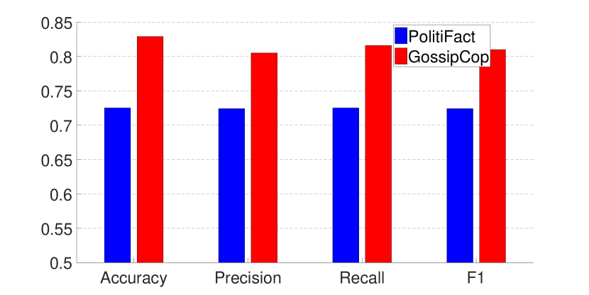
Let one dataset, e.g., PolitiFact, represent the existing data that our model has been trained on, and the other dataset, e.g., GossipCop, represent the unknown data that our model will face in the future, we find that models trained on PolitiFact do not perform well on GossipCop (Fig. 4), and vice versa (the figure for this case is omitted due to similarity).

An examination of the graphs reveals that the graphs generated from PolitiFact and GossipCop are vastly different, in terms of the numbers of nodes and edges, which explains the reason for the observed behavior.
Why not directly train on both datasets? A natural thought is to re-train the model on both datasets, but this may not be feasible, or at least not ideal in practice: there will always be new data that our model has not seen before, and it does not make sense to re-train the model from scratch on the entire data every time a new dataset is obtained, especially since as the data size grows, this can become prohibitively expensive. In the remainder of this section, we address the issue of dealing with new, unseen data.
4.1. Incremental Training
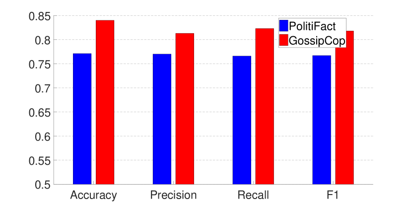
We first test incremental training, i.e., further train the model obtained from PolitiFact (or GossipCop) on the other dataset of GossipCop (or PolitiFact). However, as shown in Fig. 5, then the models only perform well on the latter dataset on which they are trained, while achieving degraded results on the former dataset (the figure for the models first trained on GossipCop and then on PolitiFact is omitted due to similarity). Note that during incremental training, we still randomly choose 75% of graphs as the training data and the rest as the test data.
This is similar to the problem of catastrophic forgetting (McCloskey and Cohen, 1989; Ratcliff, 1990; McClelland et al., 1995; French, 1999) in the field of continual learning: when a deep neural network is trained to learn a sequence of tasks, it degrades its performance on the former tasks after it learns new tasks, as the new tasks override the weights.
In our case, each new dataset can be considered as a new task. In the next subsection, we investigate how to solve the problem by applying techniques from continual learning.

4.2. Continual Learning
In order to deal with catastrophic forgetting, a number of approaches have been proposed, which can be roughly classified into three types (Parisi et al., 2018): (1) regularisation-based approaches that add extra constraints to the loss function to prevent the loss of previous knowledge; (2) architecture-based approaches that selectively train a part of the network for each task, and expand the network when necessary for new tasks; (3) dual-memory-based approaches that build on top of complementary learning systems (CLS) theory (McClelland et al., 1995; Kumaran et al., 2016), and replay samples for memory consolidation.
In this paper, we choose the following two popular methods:
-
•
Gradient Episodic Memory (GEM) (Lopez-Paz and Ranzato, 2017)—GEM uses episodic memory to store a number of samples from previous tasks, and when learning a new task , it does not allow the loss over those samples held in memory to increase compared to when the learning of task is finished;
-
•
Elastic Weight Consolidation (EWC) (Kirkpatrick et al., 2017)—its loss function consists of a quadratic penalty term on the change of the parameters, in order to prevent drastic updates to those parameters that are important to the old tasks.
In our case, the learning on the two datasets ( and ) are considered as two tasks. When the model learns the first task, it is trained as usual; then during the learning of the second task, we apply GEM and EWC:
-
•
Let be the model parameters after the first task, and be the set of instances sampled from the first dataset, then the optimisation problem under GEM becomes:
-
•
Let be the regularisation weight, be the Fisher information matrix, and be the parameters of the Gaussian distribution used by EWC to approximate the posterior of , then the loss function under EWC is:
Note that when estimating the Fisher information matrix , we sample a set of instances ( and compare the model performance under different sample sizes.
In terms of parameters, we test sample size (all the samples are chosen randomly), and (for EWC only). In addition, since the model architecture has to be consistent during the two phases (i.e., first trained on one dataset and then incrementally on the other), the number of pooling layers is set to three.
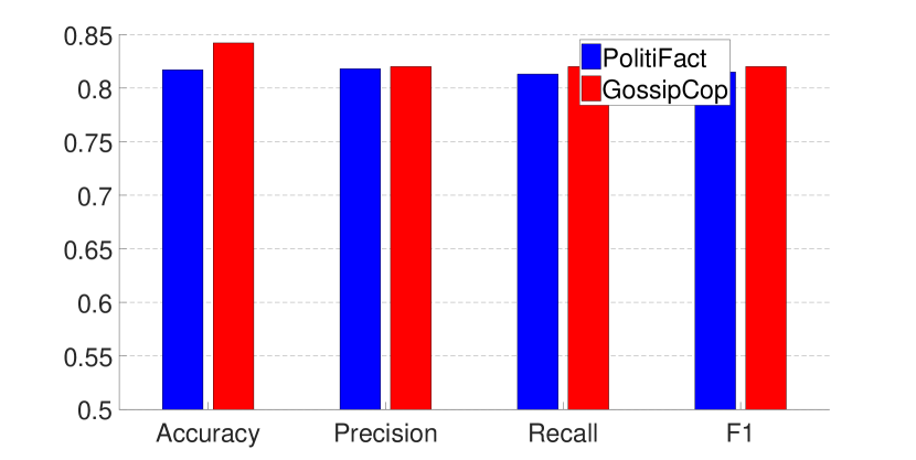
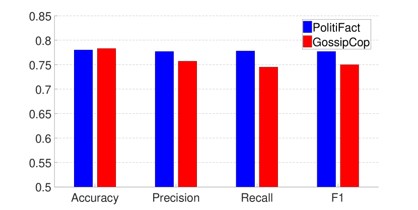
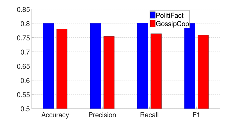
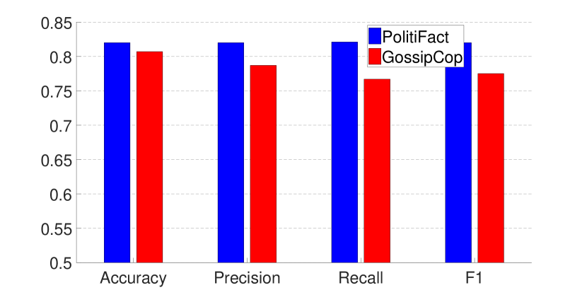
Figs. 6, 7 and Table 2 show the performance of models trained with GEM and EWC (for EWC the results when are omitted due to the space limit). The results demonstrate that while both methods can achieve a relatively balanced performance over the two datasets, GEM trained models work better than EWC trained models in general. In addition, we have also incrementally trained the model using GEM on the whole dataset, and the performance can be further improved.
Another point worth mentioning is that it requires more fine-tuning during the EWC training process. For example, we need to apply early stopping to ensure balanced results on both datasets when the model is trained with EWC.
Efficiency. In terms of efficiency, the following observations can be made from our experiments on both datasets: (1) compared with the normal training process, training with GEM and EWC requires slightly more time; (2) there is no significant difference in training time between GEM and EWC; and (3) the impact of the parameters, i.e., sample size and , on the training time is also not significant.
| Models first trained on PolitiFact | Models first trained on GossipCop | |||||||||||||||
| and then on GossipCop | and then on PolitiFact | |||||||||||||||
| PolitiFact | GossipCop | PolitiFact | GossipCop | |||||||||||||
| Acc | Pre | Rec | F1 | Acc | Pre | Rec | F1 | Acc | Pre | Rec | F1 | Acc | Pre | Rec | F1 | |
| 1 | 0.665 | 0.681 | 0.647 | 0.640 | 0.784 | 0.762 | 0.734 | 0.744 | 0.729 | 0.724 | 0.730 | 0.724 | 0.742 | 0.727 | 0.654 | 0.663 |
| 3 | 0.649 | 0.657 | 0.633 | 0.627 | 0.795 | 0.776 | 0.752 | 0.761 | 0.733 | 0.730 | 0.729 | 0.729 | 0.771 | 0.760 | 0.698 | 0.712 |
| 10 | 0.677 | 0.684 | 0.662 | 0.660 | 0.777 | 0.758 | 0.724 | 0.735 | 0.731 | 0.732 | 0.728 | 0.728 | 0.766 | 0.746 | 0.701 | 0.713 |
| 30 | 0.675 | 0.681 | 0.662 | 0.660 | 0.777 | 0.762 | 0.722 | 0.734 | 0.720 | 0.717 | 0.718 | 0.717 | 0.736 | 0.708 | 0.662 | 0.672 |
| 0.683 | 0.687 | 0.671 | 0.670 | 0.780 | 0.764 | 0.720 | 0.733 | 0.720 | 0.718 | 0.719 | 0.717 | 0.740 | 0.719 | 0.657 | 0.667 | |
| 0.689 | 0.705 | 0.672 | 0.668 | 0.778 | 0.750 | 0.739 | 0.743 | 0.729 | 0.733 | 0.729 | 0.726 | 0.759 | 0.748 | 0.680 | 0.692 | |
| 0.689 | 0.697 | 0.675 | 0.674 | 0.770 | 0.747 | 0.717 | 0.727 | 0.713 | 0.713 | 0.713 | 0.712 | 0.755 | 0.735 | 0.684 | 0.693 | |
| 0.695 | 0.703 | 0.681 | 0.680 | 0.770 | 0.745 | 0.711 | 0.722 | 0.718 | 0.720 | 0.718 | 0.717 | 0.733 | 0.704 | 0.660 | 0.669 | |
| 0.706 | 0.711 | 0.695 | 0.695 | 0.775 | 0.752 | 0.713 | 0.724 | 0.718 | 0.721 | 0.713 | 0.712 | 0.786 | 0.769 | 0.732 | 0.744 | |
| 0.726 | 0.735 | 0.714 | 0.714 | 0.761 | 0.739 | 0.697 | 0.707 | 0.722 | 0.717 | 0.715 | 0.715 | 0.764 | 0.738 | 0.705 | 0.715 | |
| 0.737 | 0.746 | 0.726 | 0.727 | 0.750 | 0.733 | 0.663 | 0.675 | 0.709 | 0.708 | 0.706 | 0.706 | 0.770 | 0.748 | 0.707 | 0.718 | |
5. Related Work
Detecting fake news on social media has been a popular research problem over recent years. In this section, we briefly review the prior work on this topic. Specifically, similar to (Shu et al., 2017; Pierri and Ceri, 2019), we classify existing work into three categories: content-based approaches, context-based approaches and mixed approaches, the first two of which, as suggested by their names, mainly rely on news content and social context to extract features for detection, respectively.
5.1. Content-based Approaches
Content-based approaches use news headlines and body content to verify the validity of the news. It can be further classified into two categories: knowledge-based and style-based (Shu et al., 2017; Zhou and Zafarani, 2018).
5.1.1. Knowledge-based Detection
In order for this type of method to work, a knowledge base or knowledge graph (Nickel et al., 2016) has to be built first. Here, knowledge can be represented in the format of a triple: (Subject, Predicate, Object), i.e., SPO triple (noa, 1999). Then, to verify an item of news, knowledge extracted from its content is compared with the facts in the knowledge graph (Wu et al., 2014; Ciampaglia et al., 2015; Shi and Weninger, 2016). If a triple is missing in the knowledge graph, different link prediction algorithms can be used to calculate the probability of an edge labelled existing from node to node .
5.1.2. Style-based Detection
According to forensic psychological studies (Undeutsch, 1967), statements based on real-life experiences differ significantly in both content and quality from those derived from fabrication or fiction. Since the purpose of fake news is to mislead the public, they often exhibit unique writing styles that are rarely seen in real news. Therefore, style-based methods aim to identify these characteristics. For example, Perez-Rosas et al. (Pérez-Rosas et al., 2018) train linear SVMs on the following linguistic features to detect fake news: unigrams, bigrams, punctuation, psycholinguistic, readability and syntax features. Other methods that fall into this category include (Horne and Adali, 2017; Volkova et al., 2017; Wang, 2017; Potthast et al., 2018).
5.2. Context-based Approaches
Social context here refers to the interactions between users, including tweet, retweet, reply, mention and follow. These engagements provide valuable information for identifying fake news spread on social media. For example, Jin et al. (Jin et al., 2016) build a stance network where the weight of an edge represents how much each pair of posts support or deny each other. Then fake news detection is based on estimating the credibility of all the posts related to the news item, which can be formalised as a graph optimisation problem.
Tacchini et al. (Tacchini et al., 2017) propose to detect fake news based on user interactions, i.e., users who liked them on Facebook. Their experiments show that both the logistic regression based and the harmonic Boolean label crowdsourcing based methods can achieve high accuracy.
Unlike the above supervised methods, an unsupervised approach is proposed in Yang et al. (Yang et al., 2019). It builds a Bayesian probability graphical model to capture the generative process among the validity of news, user opinions and user credibility.
Note that propagation-based approaches as mentioned in the introduction also belong to this category.
5.3. Mixed Approaches
Mixed approaches use both news content and associated user interactions over social media to differentiate between fake news and real news.
Ruchansky et al. (Ruchansky et al., 2017) design a three-module architecture that combines the text of a news article, the received user response and the source of the news: (1) the first module takes the user response, news content and user feature as the input, and trains a Recurrent Neural Network (RNN) to capture temporal representations of articles; (2) the second module is fed with user features to generate a score and a low-dimensional representation for each user; (3) the third module takes the output of the first two modules and trains a neural network to label the news item.
Zhang et al. (Zhang et al., 2018) propose to use a pre-extracted word set to construct explicit features from the news content, user profile and news subject description, and meanwhile use a RNN to learn latent features, such as news article content information inconsistency and profile latent patterns. Once the features are obtained, a deep diffusive network is built to learn the representations of news articles, creators and subjects.
Shu et al. (Shu et al., 2019c) use the tri-relationship among publishers, news articles and users to detect false news. Specifically, non-negative matrix factorization is used to learn the latent representations for news content and users, and the problem is formalised as an optimisation over the linear combination of each relation. Multiple machine learning algorithms are tested to solve the optimisation problem, and the results demonstrate its effectiveness.
6. Conclusions and Future Work
The prevalence of fake news over social media has become a serious social problem. In this paper, we propose a propagation-based method approach for fake news detection, which uses GNNs to distinguish between the different propagation patterns of fake news and real news over social networks. Even though the method only requires a limited number of features obtained from the social context, and does not rely on any text information, it can achieve comparable or superior performance to state-of-the-art methods that require syntactic and semantic analyses.
In addition, we identify the problem that GNNs trained on a given dataset may not perform well on new data where the graph structure is vastly different, and direct incremental training cannot solve the issue. Since this is similar to the catastrophic forgetting problem in continual learning, we propose a technique that applies two popular approaches, GEM and EWC, during the incremental training, so that balanced performance can be achieved on both existing and new data. This avoids re-training on the entire data, as it becomes prohibitively expensive as data size grows.
For future work, we will investigate whether, to some extent, the catastrophic forgetting phenomenon in this case can be mitigated by the choices of features—include more features, or find “universal” features that work well despite the different graph structures.
References
- (1)
- noa (1999) 1999. Resource Description Framework (RDF) Model and Syntax Specification. https://www.w3.org/TR/PR-rdf-syntax/
- Bian et al. (2020) Tian Bian, Xi Xiao, Tingyang Xu, Peilin Zhao, Wenbing Huang, Yu Rong, and Junzhou Huang. 2020. Rumor Detection on Social Media with Bi-Directional Graph Convolutional Networks. (2020), arXiv:2001.06362.
- Boehm (1994) Lawrence E. Boehm. 1994. The Validity Effect: A Search for Mediating Variables. Personality and Social Psychology Bulletin 20, 3 (1994), 285–293.
- Bruna et al. (2013) Joan Bruna, Wojciech Zaremba, Arthur Szlam, and Yann LeCun. 2013. Spectral Networks and Locally Connected Networks on Graphs. arXiv e-prints (2013), arXiv:1312.6203.
- Ciampaglia et al. (2015) Giovanni Luca Ciampaglia, Prashant Shiralkar, Luis M. Rocha, Johan Bollen, Filippo Menczer, and Alessandro Flammini. 2015. Computational Fact Checking from Knowledge Networks. PLOS ONE 10, 6 (2015), 1–13.
- French (1999) Robert M. French. 1999. Catastrophic forgetting in connectionist networks. Trends in Cognitive Sciences 3, 4 (1999), 128 – 135.
- Goodfellow et al. (2014) Ian J. Goodfellow, Jonathon Shlens, and Christian Szegedy. 2014. Explaining and Harnessing Adversarial Examples. eprint arXiv:1412.6572 (2014).
- Guo et al. (2018) Han Guo, Juan Cao, Yazi Zhang, Junbo Guo, and Jintao Li. 2018. Rumor Detection with Hierarchical Social Attention Network. In Proceedings of the 27th CIKM. Torino, Italy, 943–951.
- Hamilton et al. (2017) Will Hamilton, Zhitao Ying, and Jure Leskovec. 2017. Inductive Representation Learning on Large Graphs. In NIPS-2017. Curran Associates, Inc., 1024–1034.
- Horne and Adali (2017) Benjamin D. Horne and Sibel Adali. 2017. This Just In: Fake News Packs a Lot in Title, Uses Simpler, Repetitive Content in Text Body, More Similar to Satire than Real News. arXiv e-prints (2017), arXiv:1703.09398.
- Jin et al. (2016) Zhiwei Jin, Juan Cao, Yongdong Zhang, and Jiebo Luo. 2016. News Verification by Exploiting Conflicting Social Viewpoints in Microblogs. In Proceedings of the 30th AAAI (AAAI’16). Phoenix, Arizona, 2972–2978.
- Jin et al. (2017) Z. Jin, J. Cao, Y. Zhang, J. Zhou, and Q. Tian. 2017. Novel Visual and Statistical Image Features for Microblogs News Verification. TMM 19, 3 (2017), 598–608.
- keersmaecker and Roets (2017) Jonas De keersmaecker and Arne Roets. 2017. ‘Fake news’: Incorrect, but hard to correct. The role of cognitive ability on the impact of false information on social impressions. Intelligence 65 (2017), 107 – 110.
- Kim (2014) Yoon Kim. 2014. Convolutional Neural Networks for Sentence Classification. In Proceedings of the 2014 EMNLP. 1746–1751.
- Kipf and Welling (2017) Thomas N. Kipf and Max Welling. 2017. Semi-Supervised Classification with Graph Convolutional Networks. In Proceedings of the 5th ICLR. Palais des Congrès Neptune, Toulon, France.
- Kirkpatrick et al. (2017) James Kirkpatrick, Razvan Pascanu, Neil Rabinowitz, Joel Veness, Guillaume Desjardins, Andrei A. Rusu, Kieran Milan, John Quan, Tiago Ramalho, Agnieszka Grabska-Barwinska, Demis Hassabis, Claudia Clopath, Dharshan Kumaran, and Raia Hadsell. 2017. Overcoming catastrophic forgetting in neural networks. Proceedings of the National Academy of Sciences 114, 13 (2017), 3521.
- Kumaran et al. (2016) Dharshan Kumaran, Demis Hassabis, and James L. McClelland. 2016. What Learning Systems do Intelligent Agents Need? Complementary Learning Systems Theory Updated. Trends in Cognitive Sciences 20, 7 (2016), 512–534.
- Liu and Wu (2018) Yang Liu and Yi-fang Brook Wu. 2018. Early Detection of Fake News on Social Media Through Propagation Path Classification with Recurrent and Convolutional Networks. In Proceedings of the 32nd AAAI. 354–361.
- Lopez-Paz and Ranzato (2017) David Lopez-Paz and Marc’Aurelio Ranzato. 2017. Gradient Episodic Memory for Continual Learning. In NIPS-2017. Curran Associates, Inc., 6467–6476.
- Lu and Li (2020) Yi-Ju Lu and Cheng-Te Li. 2020. GCAN: Graph-aware Co-Attention Networks for Explainable Fake News Detection on Social Media. (2020), arXiv:2004.11648.
- Ma et al. (2017) Jing Ma, Wei Gao, and Kam-Fai Wong. 2017. Detect Rumors in Microblog Posts Using Propagation Structure via Kernel Learning. In 55th ACL. 708–717.
- McClelland et al. (1995) James L. McClelland, Bruce L. McNaughton, and Randall C. O’Reilly. 1995. Why there are complementary learning systems in the hippocampus and neocortex: insights from the successes and failures of connectionist models of learning and memory. Psychological Review 102, 3 (1995), 419–457.
- McCloskey and Cohen (1989) Michael McCloskey and Neal J. Cohen. 1989. Catastrophic Interference in Connectionist Networks: The Sequential Learning Problem. In Psychology of Learning and Motivation. Vol. 24. Academic Press, 109 – 165.
- Monti et al. (2019) Federico Monti, Fabrizio Frasca, Davide Eynard, Damon Mannion, and Michael M. Bronstein. 2019. Fake News Detection on Social Media using Geometric Deep Learning. arXiv e-prints (2019), arXiv:1902.06673.
- Nickel et al. (2016) M. Nickel, K. Murphy, V. Tresp, and E. Gabrilovich. 2016. A Review of Relational Machine Learning for Knowledge Graphs. Proc. IEEE 104, 1 (2016), 11–33.
- Niepert et al. (2016) Mathias Niepert, Mohamed Ahmed, and Konstantin Kutzkov. 2016. Learning Convolutional Neural Networks for Graphs. In Proceedings of the 33rd ICML - Volume 48. 2014–2023.
- Parisi et al. (2018) German I. Parisi, Ronald Kemker, Jose L. Part, Christopher Kanan, and Stefan Wermter. 2018. Continual Lifelong Learning with Neural Networks: A Review. arXiv e-prints (2018), arXiv:1802.07569.
- Pennebaker et al. (2015) James W. Pennebaker, Ryan L. Boyd, Kayla Jordan, and Kate Blackburn. 2015. The Development and Psychometric Properties of LIWC2015. Technical Report. https://repositories.lib.utexas.edu/handle/2152/31333
- Pierri and Ceri (2019) Francesco Pierri and Stefano Ceri. 2019. False News On Social Media: A Data-Driven Survey. SIGMOD Record 48, 2 (2019), 18–27.
- Popat et al. (2018) Kashyap Popat, Subhabrata Mukherjee, Andrew Yates, and Gerhard Weikum. 2018. DeClarE: Debunking Fake News and False Claims using Evidence-Aware Deep Learning. In Proceedings of the 2018 EMNLP. 22–32.
- Potthast et al. (2018) Martin Potthast, Johannes Kiesel, Kevin Reinartz, Janek Bevendorff, and Benno Stein. 2018. A Stylometric Inquiry into Hyperpartisan and Fake News. In Proceedings of the 56th ACL. 231–240.
- Pérez-Rosas et al. (2018) Verónica Pérez-Rosas, Bennett Kleinberg, Alexandra Lefevre, and Rada Mihalcea. 2018. Automatic Detection of Fake News. In Proceedings of the 27th International Conference on Computational Linguistics. 3391–3401.
- Qian et al. (2018) Feng Qian, Chengyue Gong, Karishma Sharma, and Yan Liu. 2018. Neural User Response Generator: Fake News Detection with Collective User Intelligence. In Proceedings of the 27th IJCAI. Stockholm, Sweden, 3834–3840.
- Ratcliff (1990) R. Ratcliff. 1990. Connectionist models of recognition memory: constraints imposed by learning and forgetting functions. Psychol Rev 97, 2 (1990), 285–308.
- Rubin et al. (2015) Victoria Rubin, Nadia Conroy, and Yimin Chen. 2015. Towards News Verification: Deception Detection Methods for News Discourse. In Proceedings of the 48th Hawaii International Conference on System Sciences (HICSS48).
- Ruchansky et al. (2017) Natali Ruchansky, Sungyong Seo, and Yan Liu. 2017. CSI: A Hybrid Deep Model for Fake News Detection. In Proceedings of the 26th CIKM. Singapore, 797–806.
- Shi and Weninger (2016) Baoxu Shi and Tim Weninger. 2016. Fact Checking in Heterogeneous Information Networks. In Proceedings of the 25th WWW. Montréal, Canada, 101–102.
- Shu et al. (2019a) Kai Shu, Limeng Cui, Suhang Wang, Dongwon Lee, and Huan Liu. 2019a. DEFEND: Explainable Fake News Detection. In Proceedings of the 25th KDD. 395–405.
- Shu et al. (2018) Kai Shu, Deepak Mahudeswaran, Suhang Wang, Dongwon Lee, and Huan Liu. 2018. FakeNewsNet: A Data Repository with News Content, Social Context and Spatialtemporal Information for Studying Fake News on Social Media. arXiv e-prints (2018), arXiv:1809.01286.
- Shu et al. (2019b) Kai Shu, Deepak Mahudeswaran, Suhang Wang, and Huan Liu. 2019b. Hierarchical Propagation Networks for Fake News Detection: Investigation and Exploitation. arXiv e-prints (2019), arXiv:1903.09196.
- Shu et al. (2017) Kai Shu, Amy Sliva, Suhang Wang, Jiliang Tang, and Huan Liu. 2017. Fake News Detection on Social Media: A Data Mining Perspective. SIGKDD Explorations Newsletter 19, 1 (2017), 22–36.
- Shu et al. (2019c) Kai Shu, Suhang Wang, and Huan Liu. 2019c. Beyond News Contents: The Role of Social Context for Fake News Detection. In Proceedings of the Twelfth WSDM. Melbourne, VIC, Australia, 312–320.
- Shu et al. (2020) Kai Shu, Guoqing Zheng, Yichuan Li, Subhabrata Mukherjee, Ahmed Hassan Awadallah, Scott Ruston, and Huan Liu. 2020. Leveraging Multi-Source Weak Social Supervision for Early Detection of Fake News. (2020), arXiv:2004.01732.
- Szegedy et al. (2013) Christian Szegedy, Wojciech Zaremba, Ilya Sutskever, Joan Bruna, Dumitru Erhan, Ian Goodfellow, and Rob Fergus. 2013. Intriguing Properties of Neural Networks. eprint arXiv:1312.6199 (2013).
- Tacchini et al. (2017) Eugenio Tacchini, Gabriele Ballarin, Marco L. Della Vedova, Stefano Moret, and Luca de Alfaro. 2017. Some Like it Hoax: Automated Fake News Detection in Social Networks. arXiv e-prints (2017), arXiv:1704.07506.
- Undeutsch (1967) Udo Undeutsch. 1967. Beurteilung der Glaubhaftigkeit von Aussagen. Handbuch der Psychologie, Band 11: Forensische Psychologie (1967), 26–181.
- Volkova et al. (2017) Svitlana Volkova, Kyle Shaffer, Jin Yea Jang, and Nathan Hodas. 2017. Separating Facts from Fiction: Linguistic Models to Classify Suspicious and Trusted News Posts on Twitter. In Proceedings of the 55th ACL. 647–653.
- Vosoughi et al. (2018) Soroush Vosoughi, Deb Roy, and Sinan Aral. 2018. The spread of true and false news online. Science 359, 6380 (2018), 1146–1151.
- Wang et al. (2016) Beilun Wang, Ji Gao, and Yanjun Qi. 2016. A Theoretical Framework for Robustness of (Deep) Classifiers against Adversarial Examples. arXiv:1612.00334 (2016).
- Wang (2017) William Yang Wang. 2017. “Liar, Liar Pants on Fire”: A New Benchmark Dataset for Fake News Detection. In Proceedings of the 55th ACL. 422–426.
- Wang et al. (2018) Yaqing Wang, Fenglong Ma, Zhiwei Jin, Ye Yuan, Guangxu Xun, Kishlay Jha, Lu Su, and Jing Gao. 2018. EANN: Event Adversarial Neural Networks for Multi-Modal Fake News Detection. In Proceedings of the 24th KDD. 849–857.
- Wu et al. (2015) K. Wu, S. Yang, and K. Q. Zhu. 2015. False rumors detection on Sina Weibo by propagation structures. In 2015 IEEE 31st ICDE. 651–662.
- Wu and Liu (2018) Liang Wu and Huan Liu. 2018. Tracing Fake-News Footprints: Characterizing Social Media Messages by How They Propagate. In Proceedings of the Eleventh WSDM. Marina Del Rey, CA, USA, 637–645.
- Wu et al. (2014) You Wu, Pankaj K. Agarwal, Chengkai Li, Jun Yang, and Cong Yu. 2014. Toward Computational Fact-Checking. Proc. VLDB Endow. 7, 7 (2014), 589–600.
- Wu et al. (2019) Zonghan Wu, Shirui Pan, Fengwen Chen, Guodong Long, Chengqi Zhang, and Philip S. Yu. 2019. A Comprehensive Survey on Graph Neural Networks. arXiv e-prints (2019), arXiv:1901.00596.
- Yang et al. (2019) Shuo Yang, Kai Shu, Suhang Wang, Renjie Gu, Fan Wu, and Huan Liu. 2019. Unsupervised Fake News Detection on Social Media: A Generative Approach. Proceedings of the 33rd AAAI 33 (2019), 5644–5651.
- Yang et al. (2018) Yang Yang, Lei Zheng, Jiawei Zhang, Qingcai Cui, Zhoujun Li, and Philip S. Yu. 2018. TI-CNN: Convolutional Neural Networks for Fake News Detection. arXiv e-prints (2018), arXiv:1806.00749.
- Yang et al. (2016) Zichao Yang, Diyi Yang, Chris Dyer, Xiaodong He, Alex Smola, and Eduard Hovy. 2016. Hierarchical Attention Networks for Document Classification. In Proceedings of the 2016 NAACL. 1480–1489.
- Ying et al. (2018) Rex Ying, Jiaxuan You, Christopher Morris, Xiang Ren, William L. Hamilton, and Jure Leskovec. 2018. Hierarchical Graph Representation Learning with Differentiable Pooling. In Proceedings of the 32nd NIPS. 4805–4815.
- Zhang et al. (2018) Jiawei Zhang, Bowen Dong, and Philip S. Yu. 2018. FAKEDETECTOR: Effective Fake News Detection with Deep Diffusive Neural Network. arXiv e-prints (2018), arXiv:1805.08751.
- Zhou et al. (2020) Xinyi Zhou, Jindi Wu, and Reza Zafarani. 2020. SAFE: Similarity-Aware Multi-modal Fake News Detection. In Advances in Knowledge Discovery and Data Mining. Springer International Publishing, 354–367.
- Zhou and Zafarani (2018) Xinyi Zhou and Reza Zafarani. 2018. Fake News: A Survey of Research, Detection Methods, and Opportunities. arXiv:1812.00315 [cs] (2018). arXiv:1812.00315
- Zhou and Zafarani (2019) Xinyi Zhou and Reza Zafarani. 2019. Network-based Fake News Detection: A Pattern-driven Approach. arXiv e-prints (2019), arXiv:1906.04210.