CMPCC: Corridor-based Model Predictive Contouring Control for Aggressive Drone Flight

1 Introduction

Among the criteria of designing autonomous quadrotors, generating optimized trajectories and tracking the flight paths precisely are two critical components in the action aspect. As shown in our recent work Teach-Repeat-Replan gao2020teach , a cascaded planning framework with global trajectory generation and local collision avoidance support agile flights under the user preferable routines. In work gao2020teach , though the first criteria is met by the global and local planners, the controller has no guarantees on tracking the generated motion precisely. Also, in industrial applications, the planner and controller of a quadrotor are mostly independently designed, making it hard to tune the joint performance in different applications.

Some works seo2019robust ; li2020fast attempt to compensate uncertainties introduced by disturbances, by designing error-tolerated trajectory planning methods based on Hamilton-Jacobi Reachability Analysis bansal2017hamilton . These works set handcrafted disturbance bounds, making it too conservative to find a feasible solution among dense obstacles. Tal et.al,  tal2018accurate propose control systems for accurate trajectory tracking that improves tracking accuracy. Nevertheless, they still try to track the unreachable trajectory when facing violent disturbance instead of adjusting the primary trajectory. If un-negligible disturbance occurs, local replanners such as zhou2019robust ; usenko2017real can plan motions to rejoin the reference quickly, but they are inferior to give a proper temporal distribution. The closest work to this paper liniger2015optimization applies Model predictive contouring control (MPCC) lam2010model as the planner for miniature car racing, where safety constraints are established by modeling linear functions from the boundary of the racing track. However, such constraints are not directly available for a quadrotor in unstructured environments. What’s more, due to the limited planning horizon, MPCC cannot guarantee feasibility and heavily relies on proper parameter tuning.

To bridge this gap, we propose an efficient, receding horizon, local adaptive low-level planner as the middle layer between our original planner and controller. Our method is named as corridor-based model predictive contouring control (CMPCC) since it builds upon on MPCC  lam2010model and utilizes the flight corridor as hard safety constraints. It optimizes the flight aggressiveness and tracking accuracy simultaneously, thus improving our system’s robustness by overcoming unmeasured disturbances. Our method features its online flight speed optimization, strict safety and feasibility, and real-time performance and it is released as a low-level plugin for a large variety of quadrotor systems. We summarize our contribution as follows:

1. We propose an efficient and disturbance-adaptive receding horizon low-level planner, which generates a collision-free and dynamic feasibile trajectory with adjusted temporal allocation in real time.

2. We propose a method of building appropriate constraints by constructing a forward spanning polygon tube from corresponding polyhedron and setting a terminal velocity from reference trajectory.

3. We integrate the proposed methods into a fully autonomous quadrotor system, and release our software for the reference of the community.

2 Methodology

We get the global optimized reference trajectory and the flight corridor from our previous work Teach-Repeat-Replan gao2020teach , as shown in Fig. 1.

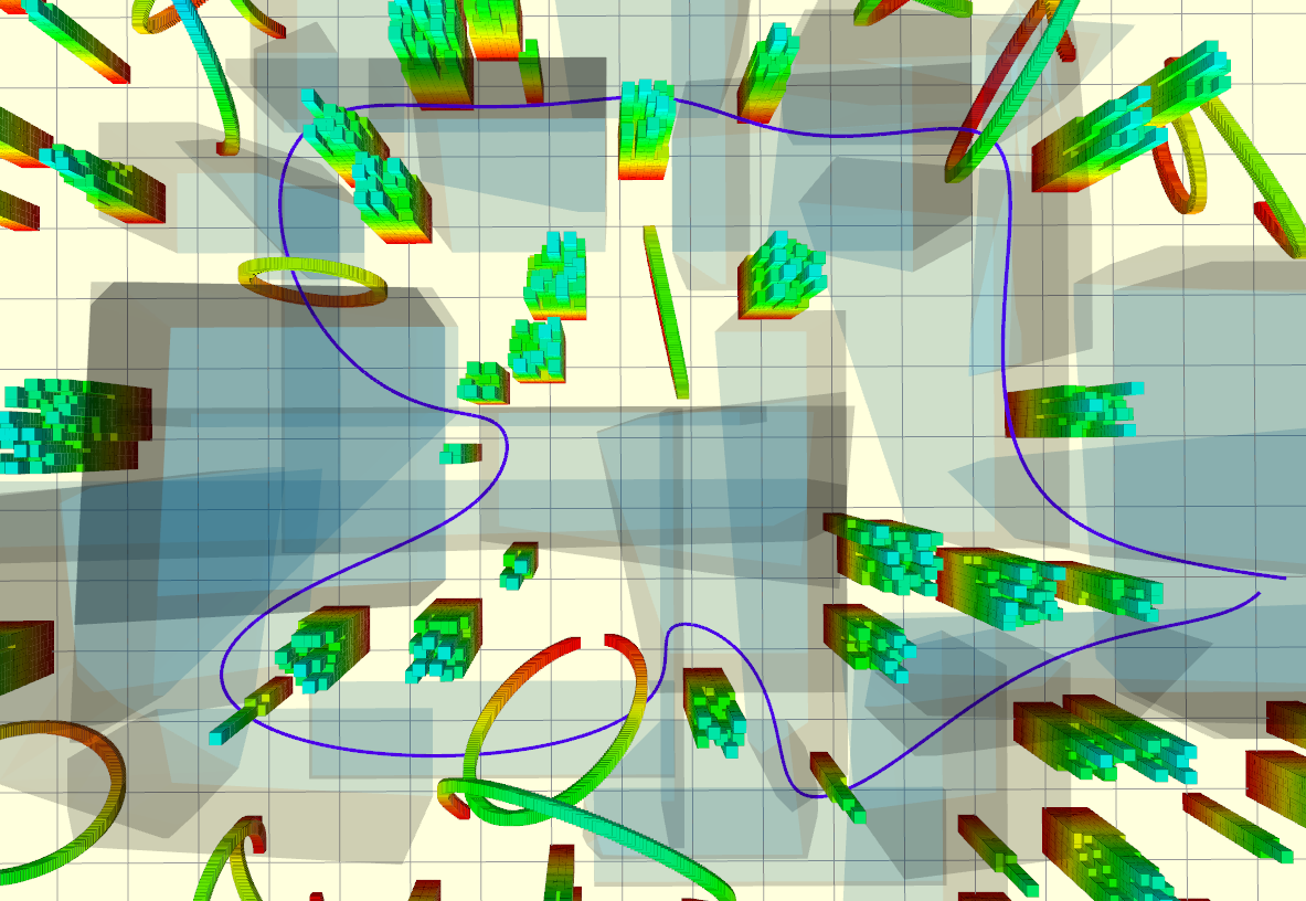
Figure 1: Global reference trajectory and Flight corridors

The global trajectory $p(t)$ is an optimized smooth curve in the space, parameterized by its original time $t$, given by

$$p=[x_{p},y_{p},z_{p}]^{T},p(t):\left[t_{0},t_{m}\right]\rightarrow\mathbb{R}^{3}.$$ (1)

We design a re-timing function $\{t(\tau):\tau\rightarrow t\}$ to map the original time variable $t$ to a new time variable $\tau$, shown in Fig. 2(a). And we also design the adjusted local trajectory $s(\tau)$, given by

$$s=[x,y,z]^{T},s(\tau):[0,\tau_{m}]\rightarrow\mathbb{R}^{3},$$ (2)

where $\tau_{m}$ is the duration of predictive horizon. The optimization objective is shown in Fig. 2(b), where $v_{p}=\dot{p}(t(\tau))$ indicates the speed of the point on global reference trajectory after re-timing, and the tracking error $e(\tau)=\left\|s(\tau)-p(t(\tau))\right\|$. The objective trades off the minimization of $\{\int_{0}^{\tau_{m}}e(\tau)d\tau\}$ and the maximization of $\{\int_{0}^{\tau_{m}}v_{p}d\tau\}$ by optimizing $t(\tau)$ and $s(\tau)$.

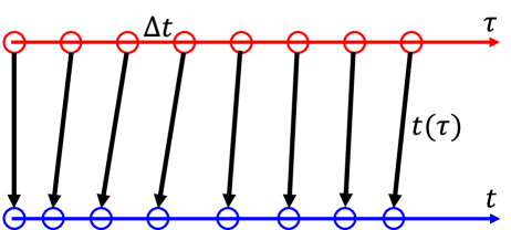
(a)

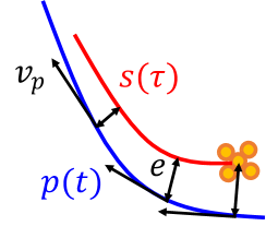
(b)

Figure 2: (a) Re-timing function (b) Components of the objective of CMPCC

Note that $v_{p}=\dot{p}(t(\tau))=p^{\prime}(t)\cdot\dot{t}(\tau)$, where $p^{\prime}(t)$ is definite according to the global trajectory $p(t)$ but $\dot{t}(\tau)$ truly indicates the traveling progress, i.e. $\dot{t}(\tau)>1$ means the drone travels faster than and $\dot{t}(\tau)<1$ means the opposing situation. Thus the objective indicating the tradeoff of tracking error $\left\|s(\tau)-p(t(\tau))\right\|$ and traveling progress $\dot{t}(\tau)$ is given by

$$J=\int_{0}^{\tau_{m}}\left(\left\|s-p\right\|^{2}-\rho\dot{t}\right)d\tau,$$ (3)

where $\rho$ is a weight of the aggressiveness. We model the system as a $3^{rd}$-order integral model and mark $v_{\mu}:=\dot{\mu}(\tau)$, $a_{\mu}:=\ddot{\mu}(\tau)$, $j_{\mu}:=\dddot{\mu}(\tau),\mu={x,y,z,t}$. Then the states and inputs of the system is given by

$$\mathbf{x}=[x,v_{x},a_{x},y,v_{y},a_{y},z,v_{z},a_{z},t,v_{t},a_{t}]^{T},$$ (4)

$$\mathbf{u}=[j_{x},j_{y},j_{z},j_{t}]^{T}.$$ (5)

They are discretized by $\Delta t$ with the length of predictive horizon $N$, and the optimization problem turns into a receding horizon MPC with linear state-transfer equations given by

$$\mathbf{x}^{(k+1)}=\mathbf{A_{d}}\mathbf{x}^{(k)}+\mathbf{B_{d}}\mathbf{u}^{(k)}$$ (6)

at the $k$-th time-step, where $\mathbf{A_{d}}$ and $\mathbf{B_{d}}$ are given by

$$\mathbf{A_{d}}=\bigoplus_{i=1}^{4}\begin{pmatrix}1&\Delta t&\frac{1}{2}\Delta t^{2}\\ 0&1&\Delta t\\ 0&0&1\\ \end{pmatrix},\mathbf{B_{d}}=\bigoplus_{i=1}^{4}\begin{pmatrix}0\\ 0\\ \Delta t\\ \end{pmatrix},$$ (7)

and the objective 3 is discretized as

$$J=\sum\limits_{k=1}^{N}\left\{\sum\limits_{\mu=x,y,z}{\left(\mu^{(k)}-\mu_{p}(t^{(k)})\right)^{2}}-\rho\cdot v_{t}^{(k)}\right\},$$ (8)

which is a nonlinear function of $\mathbf{x}$ and $\mathbf{u}$. Thanks to the framework of receding horizon, we linearize $\mu_{p}(t^{(k)})$ by

$$\mu_{p}(t^{(k)})=\mu_{p}(\theta^{(k)})+\mu_{p}^{\prime}(\theta^{(k)})\cdot\left(t^{(k)}-\theta^{(k)}\right),$$ (9)

where $\theta^{(k)}$ is the optimized result of $t^{(k+1)}$ in the last horizon. Thus the objective 8 can be represented as quadratic, given by

$$J=\sum\limits_{k=1}^{N}\left\{{\mathbf{x}^{(k)}}^{T}S_{1}^{T}Q_{k}S_{1}\mathbf{x}^{(k)}+q_{k}^{T}S_{2}\mathbf{x}^{(k)}\right\},$$ (10)

where $S_{1}$ and $S_{2}$ are selection matrices such that

$$\begin{pmatrix}x^{(k)},y^{(k)},z^{(k)},t^{(k)}\end{pmatrix}^{T}=S_{1}\mathbf{x}^{(k)},$$ (11)

$$\begin{pmatrix}x^{(k)},y^{(k)},z^{(k)},t^{(k)},v_{t}^{(k)}\end{pmatrix}^{T}=S_{2}\mathbf{x}^{(k)},$$ (12)

and

$$Q_{k}=\begin{pmatrix}1&0&0&-x^{\prime}_{p}(\theta^{(k)})\\ 0&1&0&-y^{\prime}_{p}(\theta^{(k)})\\ 0&0&1&-z^{\prime}_{p}(\theta^{(k)})\\ -x^{\prime}_{p}(\theta^{(k)})&-y^{\prime}_{p}(\theta^{(k)})&-z^{\prime}_{p}(\theta^{(k)})&\sum\limits_{\mu=x,y,z}{\mu^{\prime}_{p}(\theta^{(k)})}^{2}\\ \end{pmatrix},$$ (13)

$$q_{k}=\begin{pmatrix}2c^{(k)}_{x},2c^{(k)}_{y},2c^{(k)}_{z},\sum\limits_{\mu=x,y,z}\left\{-2\mu^{\prime}_{p}(\theta^{(k)})c^{(k)}_{\mu}\right\},-\rho\end{pmatrix}^{T},$$ (14)

$$c^{(k)}_{\mu}=\mu^{\prime}_{p}(\theta^{(k)})\cdot\theta^{(k)}-\mu_{p}(\theta^{(k)}),\mu={x,y,z}.$$ (15)

Then we construct linear inequality constraints. For a given reference point $p(\theta^{(k)})$ on the global trajectory, we define $\rm\Omega$ as the intersection of $v_{p}$’s normal plane $\rm\Phi$ with the corresponding polyhedron. As shown in Fig. 3(a), the resulting $\rm\Omega$ is a convex polygon. Then each edge of $\rm\Omega$ expands a plane sweeping along the direction of $v_{p}^{(k)}$, which gives a polygon tube, as shown in Fig. 3(b). The inner side of this tube is considered as the safe space near $p(\theta^{(k)})$ and will be modeled as inequality constraints:

$$\mathbf{C}^{(k)}\cdot[x^{(k)},y^{(k)},z^{(k)}]^{T}\leq\mathbf{b}^{(k)},k=1,2,3,...,N.$$ (16)

The sequence of the polygon tubes is shown in Fig. 4.

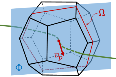
(a)

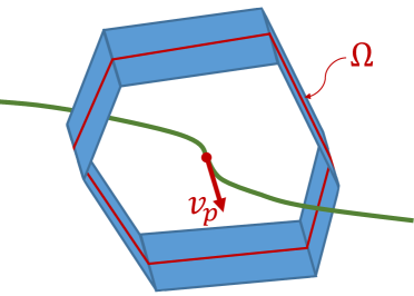
(b)

Figure 3: Generation of polygon tube

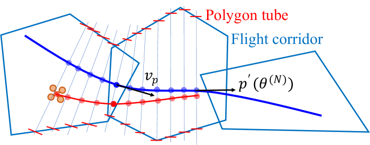
Figure 4: Sequence of linear inequality constraints for safety

In order to guarantee the dynamic feasibility, physical limits for each state are set as inequality constraints:

$$l_{x}\leq S_{3}\mathbf{x}^{(k)}\leq u_{x},$$ (17)

$$l_{u}\leq\mathbf{u}^{(k)}\leq u_{u},$$ (18)

where $l_{x},l_{u},u_{x},u_{u}$ are lower and upper bounds of velocity, acceleration and jerk at each time step. $S_{3}$ is another selection matrix such that

$$[v_{x}^{(k)},a_{x}^{(k)},v_{y}^{(k)},a_{y}^{(k)},v_{z}^{(k)},a_{z}^{(k)}]^{T}=S_{3}\mathbf{x}^{(k)}$$ (19)

In addition to physical limits for each state, a terminal velocity constraint is added such that the terminal speed should be less than $p^{\prime}(\theta^{(N)})$ in the predictive horizon. Thus, feasibility can be guaranteed since the reference trajectory is globally optimal.

The optimization problem is formulated as a standard quadratic program (QP):

$$\min\limits_{\mathbf{\bar{x}}} \mathbf{\bar{x}}^{T}Q\mathbf{\bar{x}}+q^{T}\mathbf{\bar{x}}$$ (20)

$$\mathbf{s.t.} P\mathbf{\bar{x}}=h$$ (21)

$$C\mathbf{\bar{x}}\leq b$$ (22)

where

$$\mathbf{\bar{x}}=[{\mathbf{x}^{(1)}};{\mathbf{u}^{(1)}};{\mathbf{x}^{(2)}};{\mathbf{u}^{(2)}};...;{\mathbf{x}^{(N)}};{\mathbf{u}^{(N)}}]$$ (23)

and it is solved by OSQPosqp with warm start speed-up. In practice, we choose a $1s$ predictive horizon and the sampling interval $\Delta t=0.05s$, which means $N=20$. The performance of our algorithm is tested on an Intel i7-6700 CPU, with the average solving time around 5$ms$.

3 Experiments

3.1 Experiments configuration

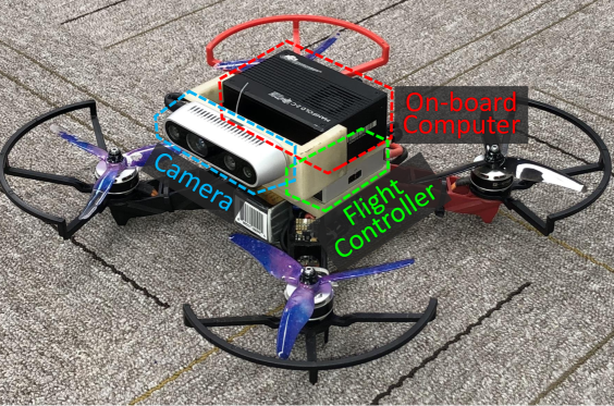
Figure 5: The hardware of the UAV

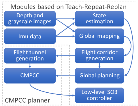
Figure 6: The Software architecture of the UAV

We use a self-developed quadrotor with an Intel Realsense D435i stereo camera and a DJI N3 flight controller for state estimation. All modules run solely on a DJI Manifold 2-C onboard computer . Our system inherits the localization, mapping and global planning from the Teach-Repeat-Replan system gao2020teach , where readers can check these modules in detail. The overall hardware and software architecture of our system is shown in Fig. 5 and Fig. 6.

3.2 Autonomous flight with contact disturbance

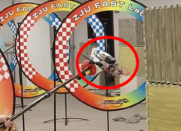
(a)

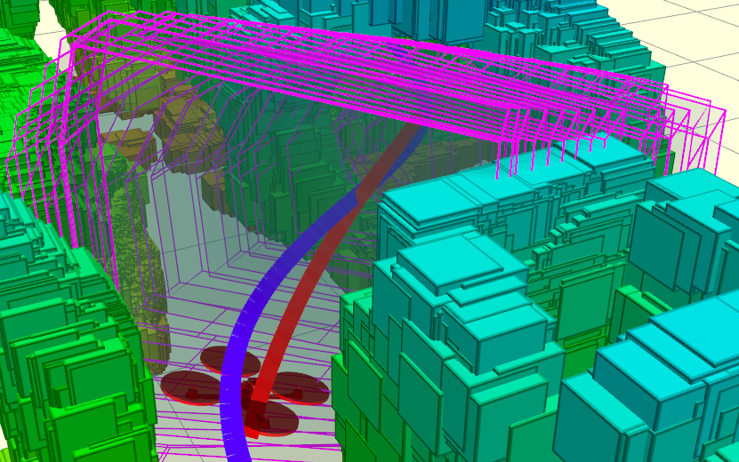
(b)

Figure 7: Circumstance of instant force disturbance

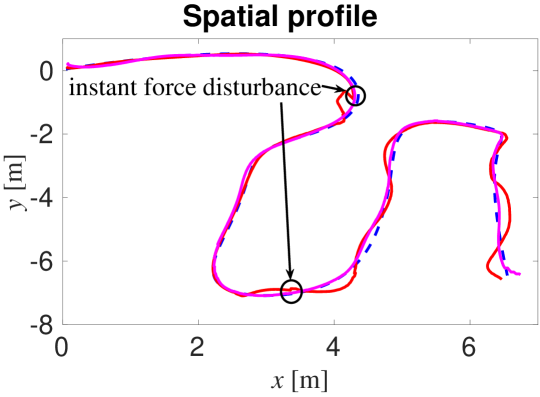
Figure 8: Spatial profile facing instant force disturbance

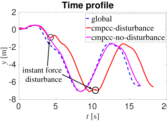
Figure 9: Time profile facing instant force disturbance

We apply challenging force disturbance to the drone to test the performance of the proposed CMPCC, as shown in Fig. 7(a). The global trajectory (blue), our locally re-planned trajectory (red), and the geometry constraints (magenta) after the hit are visualized in Fig. 7(b). As seen in the top-down view of the experiment in Fig. 8, oscillation occurs near the hit position, but the local trajectory soon converges to the global one. Also, as shown in Fig. 9, the instant force disturbance changes the temporal distribution of the optimal trajectory, resulting in the delaying of the trajectory of cmpcc (red) relative to which without disturbance (magenta) and the global trajectory (blue).

3.3 Autonomous flight with wind disturbance

We also test our method with wind disturbance by a fan, as shown in Fig. 10(a). Without the proposed CMPCC, the quadrotor tracks the global trajectory generated by Teach-Repeat-Replan with only a feedback controller, and collides with the nearby obstacle soon. However, thanks to the safety guarantee, the proposed CMPCC re-plans a safe trajectory and rejoins the global reference quickly under the wind disturbance, as shown in Fig. 10(b).

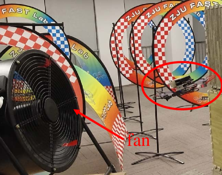
(a)

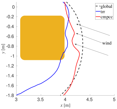
(b)

Figure 10: The circumstance of wind disturbance

The video of the experiments is available.

4 Main Experimental Insights

In practice, the flight performance of a quadrotor can be affected by many factors. Among all issues, the unexpected and unmeasurable disturbance is always an essential one for quadrotor autonomous navigation, especially for fast and aggressive flight. Recently, most autonomous quadrotor systems oleynikova2020open ; gao2020teach are developed with several independent modules include controller, planner, and perception, with the assumption that a properly designed, smooth, derivative bounded trajectory can be tracked by a controller within high bandwidth. However, this assumption does not always hold. No matter how robust the feedback controller is, it’s noted that it may fail when encountering drastic disturbance, such as immediate contact and a gust of wind, which are demonstrated in our experiments. Traditionally, people have to spend tons of time tuning the parameters of the feedback controller until a satisfactory performance. In this work, as validated by our challenging experiments, the proposed intermediate low-level replanner successfully compensates disturbances by planning local safe trajectories and automatically adjusting the flight aggressiveness. Therefore, the robustness of fast autonomous flight is improved significantly. Moreover, thanks to the convex formulation, the proposed CMPCC is solved within 5 $ms$, which suits onboard usage well.

In experiments, we also observe that the polygon tube now we use heavily depends on the static corridor. Therefore it cannot handle the variation of the environment or dynamic obstacles. In the future, we plan to investigate the way to generate safety constraints for CMPCC online.

References

- [1] Somil Bansal, Mo Chen, Sylvia Herbert, and Claire J Tomlin. Hamilton-jacobi reachability: A brief overview and recent advances. In 2017 IEEE 56th Annual Conference on Decision and Control (CDC), pages 2242–2253. IEEE, 2017.
- [2] Fei Gao, Luqi Wang, Boyu Zhou, Xin Zhou, Jie Pan, and Shaojie Shen. Teach-repeat-replan: A complete and robust system for aggressive flight in complex environments. IEEE Transactions on Robotics, 2020.
- [3] Denise Lam, Chris Manzie, and Malcolm Good. Model predictive contouring control. In 49th IEEE Conference on Decision and Control (CDC), pages 6137–6142. IEEE, 2010.
- [4] Zhichao Li, Omur Arslan, and Nikolay Atanasov. Fast and safe path-following control using a state-dependent directional metric. arXiv preprint arXiv:2002.02038, 2020.
- [5] Alexander Liniger, Alexander Domahidi, and Manfred Morari. Optimization-based autonomous racing of 1: 43 scale rc cars. Optimal Control Applications and Methods, 36(5):628–647, 2015.
- [6] Helen Oleynikova, Christian Lanegger, Zachary Taylor, Michael Pantic, Alexander Millane, Roland Siegwart, and Juan Nieto. An open-source system for vision-based micro-aerial vehicle mapping, planning, and flight in cluttered environments. Journal of Field Robotics, 37(4):642–666, 2020.
- [7] Hoseong Seo, Donggun Lee, Clark Youngdong Son, Claire J Tomlin, and H Jin Kim. Robust trajectory planning for a multirotor against disturbance based on hamilton-jacobi reachability analysis. In 2019 IEEE/RSJ International Conference on Intelligent Robots and Systems (IROS), pages 3150–3157. IEEE, 2019.
- [8] Bartolomeo Stellato, Goran Banjac, Paul Goulart, Alberto Bemporad, and Stephen Boyd. OSQP: An operator splitting solver for quadratic programs. Mathematical Programming Computation, 2020.
- [9] Ezra Tal and Sertac Karaman. Accurate tracking of aggressive quadrotor trajectories using incremental nonlinear dynamic inversion and differential flatness. In 2018 IEEE Conference on Decision and Control (CDC), pages 4282–4288. IEEE, 2018.
- [10] Vladyslav Usenko, Lukas von Stumberg, Andrej Pangercic, and Daniel Cremers. Real-time trajectory replanning for mavs using uniform b-splines and a 3d circular buffer. In 2017 IEEE/RSJ International Conference on Intelligent Robots and Systems (IROS), pages 215–222. IEEE, 2017.
- [11] Boyu Zhou, Fei Gao, Jie Pan, and Shaojie Shen. Robust real-time uav replanning using guided gradient-based optimization and topological paths. arXiv preprint arXiv:1912.12644, 2019.