ResRep: Lossless CNN Pruning via Decoupling Remembering and Forgetting

Abstract

We propose ResRep, a novel method for lossless channel pruning (a.k.a. filter pruning), which slims down a CNN by reducing the width (number of output channels) of convolutional layers. Inspired by the neurobiology research about the independence of remembering and forgetting, we propose to re-parameterize a CNN into the remembering parts and forgetting parts, where the former learn to maintain the performance and the latter learn to prune. Via training with regular SGD on the former but a novel update rule with penalty gradients on the latter, we realize structured sparsity. Then we equivalently merge the remembering and forgetting parts into the original architecture with narrower layers. In this sense, ResRep can be viewed as a successful application of Structural Re-parameterization. Such a methodology distinguishes ResRep from the traditional learning-based pruning paradigm that applies a penalty on parameters to produce sparsity, which may suppress the parameters essential for the remembering. ResRep slims down a standard ResNet-50 with 76.15% accuracy on ImageNet to a narrower one with only 45% FLOPs and no accuracy drop, which is the first to achieve lossless pruning with such a high compression ratio. The code and models are at https://github.com/DingXiaoH/ResRep.

1 Introduction

The mainstream techniques to compress and accelerate convolutional neural network (CNN) include sparsification [10, 18, 20], channel pruning [26, 27, 35], quantization [4, 5, 45, 68], knowledge distillation [28, 32, 41, 61], etc. Channel pruning [27] (a.k.a. filter pruning [34] or network slimming [42]) reduces the width (i.e., number of output channels) of convolutional layers to effectively reduce the number of floating-point operations (FLOPs) and memory footprint, which is complementary to the other model compression methods as it produces a thinner model of the original architecture with no custom structures or operations.

However, as CNN’s representational capacity depends on the width of conv layers, it is difficult to reduce the width without performance drops. On practical CNN architectures like ResNet-50 [22] and large-scale datasets like ImageNet [6], lossless pruning with high compression ratio has long been considered challenging. For reasonable trade-off between compression ratio and performance, a typical paradigm (Fig. 1.A) [2, 3, 9, 36, 39, 62, 63] trains the model with magnitude-related penalty loss (e.g., group Lasso [57, 60]) on the conv kernels to produce structured sparsity, which means all the parameters of some channels become small in magnitude. Ideally, if the parameters of pruned channels are small enough, the pruned model may deliver the same performance as before (i.e., after training but before pruning), which we refer to as perfect pruning.

Since both the training and pruning may degrade the performance, we evaluate a training-based pruning method from two aspects. 1) Resistance. The training phase tends to decrease the accuracy (referred to as training-caused damage) as it introduces some desired properties such as structured sparsity into the model, which may be harmful because the objective of optimization is changed and the parameters are deviated from the optima. We say a model has high resistance if the performance maintains high during training. 2) Prunability. When we prune the model into a smaller one after training, the properties obtained (e.g., many channels being close to zero) will reduce the pruning-caused damage. If the model endures a high pruning ratio with low performance drop, we say it has high prunability.

We desire both high resistance and prunability, but the traditional penalty-based paradigm naturally suffers from a resistance-prunability trade-off. For example, a strong group Lasso achieves high sparsity with great training-caused damage, while a weak penalty maintains the performance but results in low sparsity, hence great pruning-caused damage. Sect. 3.3 presents detailed analysis.

In this paper, we propose ResRep to address the above problem, which is inspired by the neurobiology research on remembering and forgetting. 1) Remembering requires the brain to potentiate some synapses but depotentiate the others, which resembles the training of CNN that makes some parameters large and some small. 2) Synapse elimination via shrinkage or loss of spines is one of the classical forgetting mechanisms [56] as a key process to improve efficiency in both energy and space for biological neural network, which resembles pruning. Neurobiology research reveals that remembering and forgetting are independently controlled by Rutabaga adenylyl cyclase-mediated memory formation mechanism and Rac-regulated spine shrinkage mechanism, respectively [16, 21, 59], indicating it is more reasonable to learn and prune by two decoupled modules.

Figure 1: Traditional penalty-based pruning vs. ResRep. We prune a $3\times 3$ layer with one input channel and four output channels for illustration. For the ease of visualization, we ravel the kernel $\bm{K}\in\mathbb{R}^{4\times 1\times 3\times 3}$ into a matrix $\bm{W}\in\mathbb{R}^{4\times 9}$. A) To prune some channels of $\bm{K}$ (i.e., rows of $\bm{W}$), we add a penalty loss on the kernel to the original loss, so that the gradients will make some rows smaller in magnitude, but not small enough to realize perfect pruning. B) ResRep constructs a compactor with kernel matrix $\bm{Q}\in\mathbb{R}^{4\times 4}$. Driven by the penalty gradients, the compactor selects some of its channels and generates a binary mask, which resets some of the original gradients of $\bm{Q}$ to zero. After multiple iterations, those compactor channels with reset gradients become infinitely close to zero, which enables perfect pruning. Finally, the conv-BN-compactor sequence is equivalently converted into a regular conv layer with two channels. Blank rectangles indicate zero values.

Inspired by such independence, we propose to decouple the “remembering” and “forgetting”, which are coupled in the traditional paradigm as the conv parameters are involved in both the “remembering” (objective function) and “forgetting” (penalty loss) in order for them to achieve a trade-off. That is, the traditional methods force every channel to “forget”, and remove the channels that “forgot the most”. In contrast, we first re-parameterize the original model into “remembering parts” and “forgetting parts”, then apply “remembering learning” (i.e., regular SGD with the original objective) on the former to maintain the “memory” (original performance), and “forgetting learning” on the latter to “eliminate synapses” (zero out channels).

ResRep comprises two key components: Convolutional Re-parameterization (Rep, the methodology of decoupling and the corresponding equivalent conversion) and Gradient Resetting (Res, the updage rule for “forgetting”). Specifically, we insert a compactor, which is a $1\times 1$ conv, after the original conv layer we desire to prune. During training, we add penalty gradients to only the compactors, select some compactor channels and zero out their gradients derived from the objective function. Such a training process makes some channels of compactors very close to zero, which are removed with no pruning-caused damage. Then we equivalently convert the compactor together with the preceding conv into a single conv with fewer channels through some linear transformations (Eq. 8, 9). Note that this method readily generalizes to the common case where the original conv is followed by batch normalization (BN) [31]. In this case, we append the compactor after BN, and convert the conv-BN-compactor sequence after training by first equivalently fusing the conv-BN into a conv with bias (Eq. 4). Eventually, the resultant model has the same architecture as the original (i.e., no compactors) but narrower layers (Fig. 1.B). As the equivalent conversion from the training-time model into the pruned model relies on the equivalent conversion of the parameters, ResRep can be viewed as an application of Structural Re-parameterization [11, 15, 14, 13]. The other Structural Re-parameterization works improve the VGG-like architectures [15], basic conv layers [11, 13] or an MLP-style building block [14] with different well-designed structures but all via an ordinary training process. In contrast, ResRep not only constructs extra structures (i.e., compactors) that can be equivalently converted back (Rep) but also uses a custom training strategy (Res). As will be shown in Sect. 4.3, Rep and Res are both essential: Rep constructs some structures for Res to apply on without losing the original information; Res zeros out some channels so that Rep can make the resultant conv layer narrower. Notably, ResRep can also prune a fully-connected layer because it is equivalent to a $1\times 1$ conv [46].

Algorithm 1 Pipeline of ResRep channel pruning.

1:  Input: well-trained model $\mathcal{W}$

2:  Construct the re-parameterized model $\mathcal{\hat{W}}$ with compactors. Initialize the compactors as identity matrices and the other parts with the original parameters of $\mathcal{W}$

3:  for $i=0$ to max training iterations do

4:     Forward a batch through $\mathcal{\hat{W}}$, compute the loss using the original objective function, derive the gradients

5:     Apply Gradient Resetting on the gradients of compactors only (Eq. 14)

6:     Update $\mathcal{\hat{W}}$ with the reset gradients of compactors and the original gradients of the other parameters

7:  end for

8:  Delete the rows of compactors which are close to zero (e.g., with norm $\leq 10^{-5}$) in $\mathcal{\hat{W}}$. Equivalently convert the parameters of $\mathcal{\hat{W}}$ into $\mathcal{W^{\prime}}$ (Eq. 4, 8, 3). Now $\mathcal{W^{\prime}}$ has the same architecture as $\mathcal{W}$ but narrower layers

9:  Output: pruned model $\mathcal{W^{\prime}}$

ResRep features: 1) High resistance. To maintain the performance, ResRep does not change the loss function, update rule or any training hyper-parameters of the original model (i.e., the conv-BN parts). 2) High prunability. The compactors are driven by the penalty gradients to make many channels small enough to realize perfect pruning, even with a mild penalty strength. 3) Given the required global reduction ratio of FLOPs, ResRep automatically finds the appropriate eventual width of each layer with no prior knowledge, making it a powerful tool for CNN structure optimization. 4) End-to-end training and easy implementation (Alg. 1). We summarize our contributions as:

• Inspired by the neurobiology research, we proposed to decouple “remembering” and “forgetting” for pruning.

• We proposed two techniques, Rep and Res, to achieve high resistance and prunability. They can be used separately and the combination delivers the best performance.

• We achieved state-of-the-art results on common benchmark models, including real lossless pruning on ResNet-50 on ImageNet with a pruning ratio of $54.5\%$.

2 Related Work

Pruning may refer to removing any parameters or structures from a network. Unstructured pruning [10, 18, 19, 20] can reduce the number of non-zero parameters but cannot realize speedup on common computing frameworks. Structured pruning removes some whole structures (e.g., neurons of fully-connected layers, 2D kernels, and channels), which is more friendly to hardware [40, 63]. Channel pruning is especially practical as it reduces not only the model size, the actual computations, but also the memory footprint. Pruning is related to the lottery ticket hypothesis [17]. For example, one may use ResRep to find the “winning” channels before training. Except for generic model pruning, pruning in specific contexts (e.g., the limited-data scenario [50]) has also attracted much attention.

Most of the channel pruning methods can be categorized into two families. Pruning-then-finetuning methods identify and prune the unimportant channels from a well-trained model by some measurements [1, 30, 34, 47, 51, 52, 53, 67], which may cause significant accuracy drop, and finetune it afterwards. Some methods repeat pruning-finetuning iterations to measure the importance and prune progressively [8, 37]. A major drawback is that the pruned models can be easily trapped into bad local minima, and sometimes cannot even reach a similar level of accuracy with a counterpart of the same structure trained from scratch [44]. This discovery highlights the significance of perfect pruning, which eliminates the need for finetuning. In this family, PCAS [66] is the most related to ResRep, which identifies the unimportant channels by training attention modules appended after conv layers. Unlike ResRep, PCAS performs imperfect pruning and requires finetuning after removing the unimportant channels. Moreover, PCAS discards the attention modules after training, which results in more structural damage, while ResRep uses a mathematically equivalent transformation to obtain the final model structure without any performance drop. Learning-based pruning methods utilize a custom learning process to reduce the pruning-caused damage. Apart from the above-mentioned penalty-based paradigm to zero out some of the channels [2, 3, 9, 36, 39, 62, 63], some other methods prune via making some filters identical [12], meta-learning [43], adversarial learning [38], etc.

3 ResRep for Lossless Channel Pruning

3.1 Formulation and Background

We first introduce the formulation of conv and channel pruning. Let $D$ and $C$ be the output and input channels, $K$ be the kernel size, $\bm{K}\in\mathbb{R}^{D\times C\times K\times K}$ be the kernel parameter tensor, $\bm{b}\in\mathbb{R}^{D}$ be the optional bias, $I\in\mathbb{R}^{N\times C\times H\times W}$ and $\bm{O}\in\mathbb{R}^{N\times D\times H^{\prime}\times W^{\prime}}$ be the input and output, $\circledast$ be the convolution operator, and $B$ be the broadcast function which replicates $\bm{b}$ into $N\times D\times H^{\prime}\times W^{\prime}$, we have

$$\bm{O}=\bm{I}\circledast\bm{K}+B(\bm{b})\,.$$ (1)

For a conv layer with no bias term but a following batch normalization (BN) [31] layer with mean $\bm{\mu}$, standard deviation $\bm{\sigma}$, scaling factor $\bm{\gamma}$ and bias $\bm{\beta}\in\mathbb{R}^{D}$, we have

$$\bm{O}_{:,j,:,:}=((\bm{I}\circledast\bm{K})_{:,j,:,:}-\mu_{j})\frac{\gamma_{j}}{\sigma_{j}}+\beta_{j}\,,\forall 1\leq j\leq D\,.$$ (2)

Let $i$ be the index of conv layer. To prune conv $i$, we obtain the index set of pruned channels $\mathcal{P}^{(i)}\subset\{1,2,\dots,D\}$ according to some rules, then its complementary set $\mathcal{S}^{(i)}=\{1,2,\dots,D\}\setminus\mathcal{P}^{(i)}$ for the index set of channels which survive. The pruning operation preserves the $\mathcal{S}^{(i)}$ output channels of conv $i$ and the corresponding input channels of the succeeding layer (conv $i+1$), and discard the others. The corresponding entries in the bias or following BN, if any, should be discarded as well. The obtained kernels are

$$\bm{K}^{(i)\prime}=\bm{K}^{(i)}_{\mathcal{S}^{(i)},:,:,:}\,,\quad\bm{K}^{(i+1)\prime}=\bm{K}^{(i+1)}_{:,\mathcal{S}^{(i)},:,:}\,.$$ (3)

3.2 Convolutional Re-parameterization

For every conv layer together with the following BN (if any) we desire to prune, which are referred to as the target layers, we append a compactor ($1\times 1$ conv) with kernel $\bm{Q}\in\mathbb{R}^{D\times D}$. Given a well-trained model $\mathcal{W}$, we construct a re-parameterized model $\mathcal{\hat{W}}$ by initializing the conv-BN as the original weights of $\mathcal{W}$ and $\bm{Q}$ as an identity matrix, so that the re-parameterized model produces the identical outputs as the original. Note that if the target layer has no following BN, the “BN” in our notation can be safely viewed as a bias. After training with Gradient Resetting, which will be described in detail in Sect. 3.3, we prune the resulting close-to-zero channels of compactors and convert the model into $\mathcal{W}^{\prime}$, which has the same architecture as $\mathcal{W}$ but narrower layers. Concretely, for a specific compactor with kernel $\bm{Q}$, we prune the channels with norm smaller than a threshold $\epsilon$. Formally, we obtain the to-be-pruned set by $\mathcal{P}=\{j\,|\,||\bm{Q}_{j,:}||_{2}<\epsilon\}$, or the surviving set $\mathcal{S}=\{j\,|\,||\bm{Q}_{j,:}||_{2}\geq\epsilon\}$. Similar to Eq. 3, we prune $\bm{Q}$ by $\bm{Q}^{\prime}=\bm{Q}_{\mathcal{S},:}$. In our experiments, we use $\epsilon=10^{-5}$, which is found to be small enough to realize perfect pruning. After pruning, the compactor has fewer rows than columns, i.e., $\bm{Q}^{\prime}\in\mathbb{R}^{D^{\prime}\times D},D^{\prime}=|\mathcal{S}|$. To convert $\mathcal{\hat{W}}$ into $\mathcal{W}^{\prime}$, we seek to convert every conv-BN-compactor sequence into a conv layer with $\bm{K}^{\prime}\in\mathbb{R}^{D^{\prime}\times C\times K\times K}$ and bias $\bm{b}^{\prime}\in\mathbb{R}^{D^{\prime}}$.

Firstly, we equivalently fuse a conv-BN into a conv for inference, which produces the identical outputs as the original. With $\bm{K},\bm{\mu},\bm{\sigma},\bm{\gamma},\bm{\beta}$ of a conv-BN, we construct a new conv with kernel $\bar{\bm{K}}$ and bias $\bar{\bm{b}}$ as follows. For $1\leq j\leq D$,

$$\bar{\bm{K}}_{j,:,:,:}=\frac{\gamma_{j}}{\sigma_{j}}\bm{K}_{j,:,:,:}\,,\quad\bar{b}_{j}=-\frac{\mu_{j}\gamma_{j}}{\sigma_{j}}+\beta_{j}\,.$$ (4)

Given Eq. 1, 2 and the homogeneity of conv, we can verify

$$((\bm{I}\circledast\bm{K})_{:,j,:,:}-\mu_{j})\frac{\gamma_{j}}{\sigma_{j}}+\beta_{j}=(\bm{I}\circledast\bar{\bm{K}}+B(\bar{\bm{b}}))_{:,j,:,:}\,.$$ (5)

Then we seek for the formula to construct $\bm{K}^{\prime}$ and $\bm{b}^{\prime}$ so that

$$(\bm{I}\circledast\bar{\bm{K}}+B(\bar{\bm{b}}))\circledast\bm{Q}^{\prime}=\bm{I}\circledast\bm{K}^{\prime}+B(\bm{b}^{\prime})\,.$$ (6)

With the additivity of convolution, we arrive at

$$\bm{I}\circledast\bar{\bm{K}}\circledast\bm{Q}^{\prime}+B(\bar{\bm{b}})\circledast\bm{Q}^{\prime}=\bm{I}\circledast\bm{K}^{\prime}+B(\bm{b}^{\prime})\,.$$ (7)

We note that very channel of $B(\bar{\bm{b}})$ is a constant matrix, thus every channel of $B(\bar{\bm{b}})\circledast\bm{Q}^{\prime}$ is also a constant matrix. As the $1\times 1$ conv with $\bm{Q}^{\prime}$ on $\bm{I}\circledast\bar{\bm{K}}$ only performs cross-channel recombination, we can merge $\bm{Q}^{\prime}$ into $\bar{\bm{K}}$ by recombining the entries in $\bar{\bm{K}}$. Let $T$ be the transpose function (e.g., $T(\bar{\bm{K}})$ is $C\times D\times K\times K$), we present the formulas to construct $\bm{K}^{\prime}$ and $\bm{b}^{\prime}$, which can be easily verified.

$$\bm{K}^{\prime}=T(T(\bar{\bm{K}})\circledast\bm{Q}^{\prime})\,,$$ (8)

$$b^{\prime}_{j}=\bar{\bm{b}}\cdot\bm{Q}^{\prime}_{j,:}\,,\quad\forall 1\leq j\leq D^{\prime}\,.$$ (9)

In practice, we convert and save the weights of the trained re-parameterized model, construct a model with the original architecture but narrower layers without BN, and use the saved weights for testing and deployment.

3.3 Gradient Resetting

We describe how to produce structured sparsity in compactors while maintaining the accuracy, beginning by discussing the traditional usage of penalty on a specific kernel $\bm{K}$ to make the magnitude of some channels smaller, i.e., $||\bm{K}_{\mathcal{P},:,:,:}||\to 0$. Let $\bm{\Theta}$ be the universal set of parameters, $X,Y$ be the data examples and labels, $L_{\text{perf}}(X,Y,\bm{\Theta})$ be the performance-related objective function (e.g., cross-entropy for classification). The traditional paradigm adds a penalty term $P(\bm{K})$ by a pre-defined strength factor $\lambda$,

$$L_{\text{total}}(X,Y,\bm{\Theta})=L_{\text{perf}}(X,Y,\bm{\Theta})+\lambda P(\bm{K})\,,$$ (10)

where the common forms of $P$ include L1 [34], L2 [9], and group Lasso [39, 63]. Specifically, group Lasso is effective in producing channel-wise structured sparsity. In the following discussions, we denote a specific channel in $\bm{K}$ by $\bm{F}^{(j)}=\bm{K}_{j,:,:,:}$. Then the group Lasso loss is formulated as

$$P_{\text{Lasso}}(\bm{K})=\sum_{j=1}^{D}||\bm{F}^{(j)}||_{E}\,,$$ (11)

where $||\bm{F}^{(j)}||_{E}$ is the Euclidean norm

$$||\bm{F}||_{E}=\sqrt{\sum_{c=1}^{C}\sum_{p=1}^{K}\sum_{q=1}^{K}\bm{F}_{c,p,q}^{2}}\,.$$ (12)

With $G(\bm{F})$ as the gradient, we take the derivative,

$$G(\bm{F})=\frac{\partial L_{\text{total}}(X,Y,\bm{\Theta})}{\partial\bm{F}}=\frac{\partial L_{\text{perf}}(X,Y,\bm{\Theta})}{\partial\bm{F}}+\lambda\frac{\bm{F}}{||\bm{F}||_{E}}\,.$$ (13)

The training dynamics of a specific channel $\bm{F}$ are quite straightforward. Beginning from a well-trained model, $\bm{F}$ resides near the local optima, thus the first term of Eq. 13 is close to $\bm{0}$ but the second is not, so $\bm{F}$ is pushed closer to $\bm{0}$. If $\bm{F}$ is important to the performance, the objective function will intend to maintain its magnitude, i.e., the first gradient term will compete against the second, thus $\bm{F}$ will end up smaller than it used to be, depending on $\lambda$. Otherwise, taking the extreme case for example, if $\bm{F}$ does not influence $L_{\text{perf}}$ at all, the first term will be $\bm{0}$, so $\bm{F}$ will keep growing towards $\bm{0}$ by the second term. In other words, the performance-related loss and the penalty loss compete so that the resulting value of $\bm{F}$ will reflect its importance, which we refer to as competence-based importance evaluation for convenience. However, we face a dilemma. Problem A: The penalty deviates the parameters of every channel from the optima of the objective function. Notably, a mild deviation may not bring negative effects, e.g., L2 regularization can also be viewed as a mild deviation. However, with a strong penalty, though some channels are zeroed out for pruning, the remaining channels are also made too small to maintain the representational capacity, which is an undesired side-effect. Problem B: With mild penalty for the high resistance, we cannot achieve high prunability, because most of the channels merely become closer to $\bm{0}$ than they used to be, but not close enough for perfect pruning.

We propose to achieve high prunability with a mild penalty by resetting the gradients derived from the objective function. We introduce a binary mask $m\in\{0,1\}$, which indicates whether we wish to zero out $\bm{F}$. For the ease of implementation, we add no terms to the objective function (i.e., $L_{\text{total}}=L_{\text{perf}}$), simply derive the gradients as usual, and then manually apply the mask, add the penalty gradients and use the resultant gradients for SGD update:

$$G(\bm{F})\leftarrow\frac{\partial L_{\text{perf}}(X,Y,\bm{\Theta})}{\partial\bm{F}}m+\lambda\frac{\bm{F}}{||\bm{F}||_{E}}\,.$$ (14)

We will describe how to decide which channels to zero out (i.e., set mask values for multiple channels) in the next section. In this way, we have solved the above two problems. A) Though we add Lasso gradients to the objective-related gradients of every channel, which is equivalent to deviating the optima by adding Lasso loss to the original loss, the deviation is mild ($\lambda=10^{-4}$ in our experiments) hence harmless to the performance. B) With $m=0$, the first term no longer exists to compete against the second, thus even a mild $\lambda$ can make $\bm{F}$ steadily move towards $\bm{0}$.

3.4 The Remembering Parts Remember Always,
the Forgetting Parts Forget Progressively

If directly used on conv kernels, Res brings a problem: some objective-related gradients encode the supervision information for maintaining the performance but are discarded. Intuitively, the parameters are forced to “forget” some useful information (gradients). Fortunately, Rep is exactly the solution, which allows us to prune the compactors only, not the original conv layers. ResRep only forces the compactors to “forget”, and all the other layers still focus on “remembering”, so we will not lose the information encoded in the gradients of the original kernels.

To combine Res with Rep, we need to decide which channels of $\bm{Q}$ to be zeroed out. When training the re-parameterized model, we add the Lasso gradients to the compactors only. After a few epochs, $||\bm{Q}_{j,:}||$ will reflect the importance of channel $j$ (competence-based importance evaluation discussed in the Sect. 3.3), so we start to perform channel selection based on the value of $\bm{Q}$. Let $n$ be the number of compactors, $\bm{m}^{(i)}$ (a $D^{(i)}$-dimensional binary vector) be the mask for the $i$-th compactor, we define $\bm{t}^{(i)}\in\mathbb{R}^{D^{(i)}}$ as the metric vector,

$$t^{(i)}_{j}=||\bm{Q}^{(i)}_{j,:}||_{2}\,,\quad\forall 1\leq j\leq D^{(i)}\,.$$ (15)

For each time of channel selection, we calculate the metric values for every channel in every compactor and organize them as a mapping $\mathcal{M}=\{(i,j)\to t^{(i)}_{j}\,|\,\forall 1\leq i\leq n,1\leq j\leq D^{(i)}\}$. Then we sort the values of $\mathcal{M}$ in ascending order, start to pick one at a time from the smallest, and set the corresponding mask $m^{(i)}_{j}$ to 0. We stop picking when the reduced FLOPs reaches our target, or we have already picked $\theta$ (named the channel selection limit) channels. The mask values of unpicked channels are set to 1. The motivation is straightforward: following the discussions of competence-based importance evaluation, just like the traditional usage of penalty loss to compete against the original loss and select the channels with smaller norms, we use the penalty gradients to compete with the original gradients. Even better, all the metric values are 1 at the beginning (because every compactor kernel is initialized as an identity matrix), making it fair to compare them among different layers. We initialize $\theta$ as a small number, increase $\theta$ every several iterations and re-select channels to “forget” progressively, avoiding zeroing out too many channels at once. As Fig. 4 shows, those mask-0 channels will become very close to $\bm{0}$, thus the structured sparsity emerges in compactors.

4 Experiments

4.1 Datasets, Models and Settings

We use ResNet-50 and MobileNet [29] on ImageNet-1K. For the reproducibility, we follow the data augmentation of PyTorch official example [54] including random cropping and flipping. For ResNet-50, we use the official torchvision base model (76.15% top-1 accuracy) [55] for the fair comparison with most competitors. For MobileNet, we train from scratch with an initial learning rate of 0.1, batch size of 512 and cosine learning rate annealing for 70 epochs. The top-1 accuracy is 70.78%, slightly higher than that reported in the original paper. We use ResNet-56/110 on CIFAR-10 [33] with the standard data augmentation [22]: padding to $40\times 40$, random cropping and flipping. We train the base models with batch size of 64 and the common learning rate schedule which is initialized as 0.1, multiplied by 0.1 at epoch 120 and 180, and terminated after 240 epochs. We count the FLOPs as multiply-adds, which is 4.09G for ResNet-50 [55], 569M for MobileNet, and 126M/253M for ResNet-56/110.

4.2 Pruning Results on ImageNet and CIFAR-10

Table 1: Pruning results of ResNet-50 and MobileNet on ImageNet.

Model	Result	Base Top-1	Base Top-5	Pruned Top-1	Pruned Top-5	Top-1 $\downarrow$	Top-5 $\downarrow$	FLOPs $\downarrow$%
ResNet-50	SFP [24]	76.15	92.87	74.61	92.06	1.54	0.81	41.8
	GAL-0.5 [38]	76.15	92.87	71.95	90.94	4.20	1.93	43.03
	NISP [67]	-	-	-	-	0.89	-	44.01
	Taylor-FO-BN [51]	76.18	-	74.50	-	1.68	-	44.98
	Channel Pr [27]	-	92.2	-	90.8	-	1.4	50
	HP [64]	76.01	92.93	74.87	92.43	1.14	0.50	50
	MetaPruning [43]	76.6	-	75.4	-	1.2	-	51.10
	Autopr [49]	76.15	92.87	74.76	92.15	1.39	0.72	51.21
	GDP [37]	75.13	92.30	71.89	90.71	3.24	1.59	51.30
	FPGM [26]	76.15	92.87	74.83	92.32	1.32	0.55	53.5
	ResRep	76.15	92.87	76.15$\pm$0.01	92.89$\pm$0.04	0.00	-0.02	54.54
	C-SGD (extension) [12]	76.15	92.87	75.29	92.39	0.86	0.48	55.44
	DCP [69]	76.01	92.93	74.95	92.32	1.06	0.61	55.76
	C-SGD [7]	75.33	92.56	74.54	92.09	0.79	0.47	55.76
	ThiNet [48]	75.30	92.20	72.03	90.99	3.27	1.21	55.83
	SASL [58]	76.15	92.87	75.15	92.47	1.00	0.40	56.10
	ResRep	76.15	92.87	75.97$\pm$0.02	92.75$\pm$0.01	0.18	0.12	56.11
	TRP [65]	75.90	92.70	72.69	91.41	3.21	1.29	56.52
	LFPC [23]	76.15	92.87	74.46	92.32	1.69	0.55	60.8
	HRank [35]	76.15	92.87	71.98	91.01	4.17	1.86	62.10
	ResRep	76.15	92.87	75.30$\pm$0.01	92.47$\pm$0.01	0.85	0.40	62.10
MobileNet	MetaPruning [43]	70.6	-	66.1	-	4.5	-	73.81
	ResRep	70.78	89.78	68.02$\pm$0.02	87.66$\pm$0.02	2.76	2.12	73.91

We apply ResRep on ResNet-50 and MobileNet with the same hyper-parameters: $\lambda=10^{-4}$, batch size=256, initial learning rate=0.01 and cosine annealing for 180 epochs. We set the channel selection limit $\theta=4$ and $\theta\leftarrow\theta+4$ every 200 batches and the first channel selection begins after 5 epochs. That is, after a 5-epoch “warm-up”, we pick up 4 channels with the lowest $t$ values among all the layers and then pick 4 more channels every 200 batches, until we reach the FLOPs reduction target. For the ease of comparison, we experiment with ResNet-50 for three times with FLOPs reduction target of 54.5% (1% higher than FPGM [26]), 56.1% (SASL [58]) and 62.1% (HRank [35]), respectively, and MobileNet with 73.9% to compare with MetaPruning [43]. Following most competitors, we prune the first ($1\times 1$) and second ($3\times 3$) conv layers in every residual block of ResNet-50, and every non-depthwise conv of MobileNet. Inspired by a prior work [10] which zeros out some gradients and utilizes momentum and weight decay for CNN sparsification, we raise the SGD momentum coefficient on compactors from 0.9 (the default setting in most cases) to 0.99. Intuitively, the mask-0 channels continuously grow in the same direction (i.e., towards zero), and such a tendency accumulates in the momentum, thus the zeroing-out process can be accelerated by a larger momentum coefficient. For ResNet-56/110, the target layers include the first layers of residual block, and we use the same hyper-parameters as ImageNet except batch size of 64 and 480 training epochs.

Table 2: Pruning results of ResNet-56/110 on CIFAR-10.

Model	Result	Base Top-1	Pruned Top-1	Top-1 $\downarrow$%	FLOPs $\downarrow$%
R56	AMC [25]	92.8	91.9	0.9	50
	FPGM [26]	93.59	93.26	0.33	52.6
	SFP [24]	93.59	93.35	0.24	52.6
	LFPC [23]	93.59	93.24	0.35	52.9
	ResRep	93.71	93.71$\pm$0.02	0.00	52.91
	TRP [65]	93.14	91.62	1.52	77.82
	ResRep	93.71	92.66$\pm$0.07	1.05	77.83
R110	Li et al. [34]	93.53	93.30	0.23	38.60
	GAL-0.5 [38]	93.50	92.74	0.76	48.5
	HRank [35]	93.50	93.36	0.14	58.2
	ResRep	94.64	94.62$\pm$0.04	0.02	58.21

Table. 1, 2 show the superiority of ResRep. Our results are average of 3 runs on ImageNet and 5 runs on CIFAR. On ResNet-50, ResRep achieves 0.00% top-1 accuracy drop, which is the first to realize lossless pruning with such high pruning ratio (54.54%), to the best of our knowledge. In terms of top-1 accuracy drop, ResRep outperforms SASL by 0.82%, HRank by 3.32% and all the other recent competitors by a large margin. On MobileNet, ResRep outperforms MetaPruning by 1.77%. On ResNet-56/110, ResRep also outperforms, even though the comparison on accuracy drop is biased towards other methods, as our base models have higher accuracy (i.e., it is more challenging to prune a higher-accuracy model without accuracy degradation).

The final width of each target layer (Fig. 3) shows that ResRep discovers the appropriate final structure without any prior knowledge, given the desired global pruning ratio. Notably, ResRep chooses to preserve more channels at higher-level layers of ResNet-50 and MobileNet, but prunes aggressively on the last blocks of ResNet-56. An explanation is that rich higher-level features are essential for maintaining the fitting capacity on difficult task like ImageNet, while ResNet-56 suffers from over-fitting on CIFAR-10.

Figure 2: Training loss (left) and validation accuracy (right) of pruned-finetuned and ResRep on ResNet-50.

Table 3: ResNet-50 baselines and variants of ResRep.

	Top-1 acc	FLOPs $\downarrow$%
1) Base model finetuned	76.19	-
2) Uniformly shrunk baseline	74.39	55.4
3) Pruned-finetuned	74.66	54.5
4) Vector re-parameterization	75.57	54.5
5) Momentum on compactors as 0.9	75.05	45.1

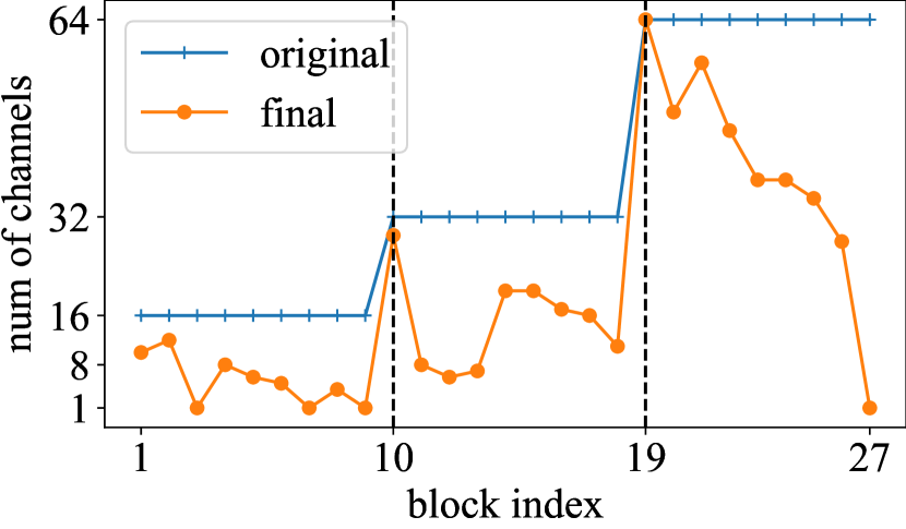
Figure 3: Width of target layers in pruned models. Left: ResNet-50 with the first $1\times 1$ and $3\times 3$ layer in each block shown separately. Middle: MobileNet. Right: ResNet-56. Vertical dashed lines indicate the stage transition in ResNets.

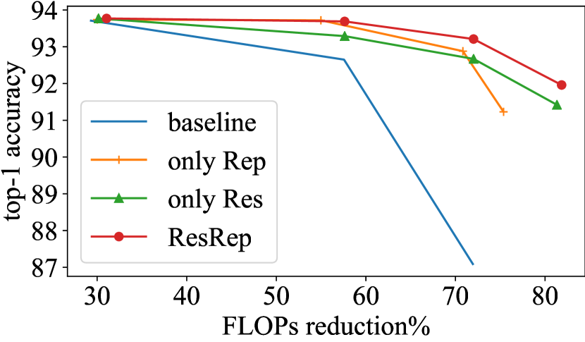
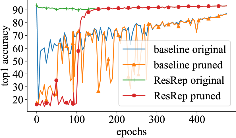
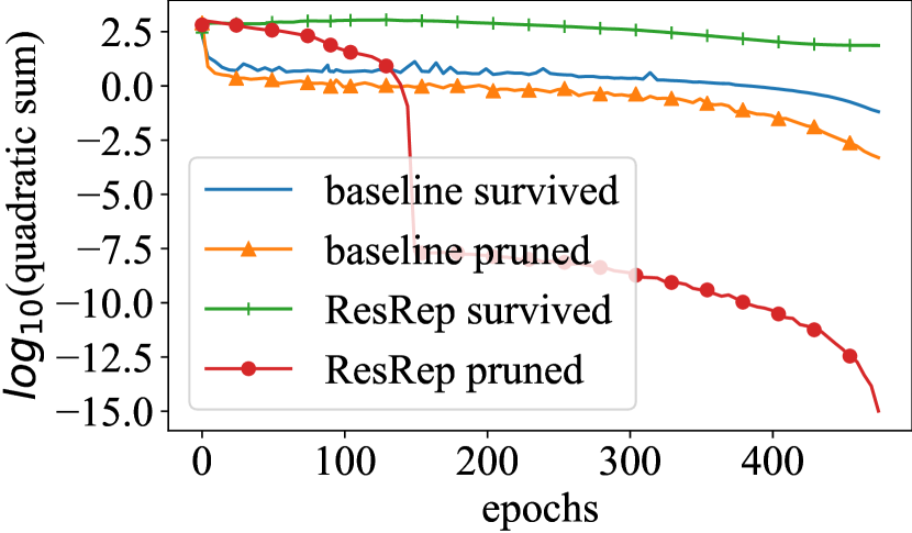
Figure 4: Left: FLOPs reduction v.s. accuracy of baseline, Res, Rep and ResRep. Middle: the original and pruned accuracy every 5 epochs. Right: the quadratic sum of survived parameters and those to-be-pruned (note the logarithmic scale).

We construct a series of baselines and variants of ResRep for comparison (Table. 3). 1) The base model is further finetuned with the same learning rate schedule for 180 epochs, and the accuracy is merely lifted by 0.04%, suggesting the performance of ResRep is not simply due to the effect of training settings. 2) We construct a uniformly shrunk baseline by building a ResNet-50 where all the target layers are reduced to 1/2 of the original width, thus the FLOPs is reduced by 55.4%. We train it from scratch with the same training settings as the base model, and the final accuracy is 74.39%, which is 1.58% lower than our 56.1%-pruned model. 3) We compare ResRep against a classic pruning-then-finetuning method by sorting all the channels of base model by their Euclidean norm, pruning from the smallest until 54.5% reduction ratio, and finetuning the resultant model with the same 180-epoch setting. Not surprisingly, the finetuned model is hardly better than the shrunk baseline trained from scratch. The training loss and validation accuracy (Fig. 2) shows the pruned model recovers quickly but cannot reach a comparable accuracy as the 54.5%-pruned ResRep model. This observation is consistent with a prior study that a pruned model may be easily trapped into bad local minima [44]. 4) A straightforward alternative of re-parameterization to verify the significance of Convolutional Re-parameterization. It changes the form of compactor from $1\times 1$ conv to a $D$-dimensional trainable vector (i.e., a channel-wise scaling layer) initialized as $\bm{1}$, and the Lasso penalty naturally degrades to L1. After training with the same settings as the 54.5%-pruned model for 180 epochs, the final accuracy is 75.57%, which is 0.58% lower. Intuitively, re-parameterization with $1\times 1$ conv folds the original kernel into a lower-dim kernel (i.e., re-combines the channels), but a vector simply deletes some channels. 5) We verify the necessity of 0.99-momentum by setting the momentum of compactors as 0.9, and fewer channels end up close to zero (below $\epsilon=10^{-5}$). Though a higher momentum reduces parameters faster, it is not necessary if longer training time is acceptable.

4.3 Ablation Studies

We then perform controlled experiments with the same training configurations as described above on ResNet-56 to evaluate Rep and Res separately. As the baseline, we adopt the traditional paradigm by directly adding Lasso loss (Eq. 11) on all the target layers. With $\lambda\in\{0.3,0.03,0.003,0.001\}$, we obtain four models with different final accuracy: 69.81%, 87.09%, 92.65%, 93.69%. To realize perfect pruning on each trained model, we attain the minimal structure by removing the channels one at a time until the accuracy drops below the original (i.e., pruning any one more channel of the minimal structure will decrease the accuracy). Then we record the FLOPs reduction of the minimal structures: 81.24%, 71.94%, 57.56%, 28.31%. We test Rep but no Res by applying Lasso loss on the compactors with varying $\lambda$ to achieve comparable FLOPs reduction as baselines. And with Res but no Rep, we directly apply Gradient Resetting on the original conv kernels, targeting at the same FLOPs reduction as the four baseline models. Then we experiment with the full-featured ResRep. As shown in the left of Fig. 4 (the baseline data point of (81.24%, 69.81%) is ignored for better readability), Res and Rep deliver better final accuracy than the baselines, and perform even better when combined.

We investigate into the training process by saving the parameters of the $\lambda=0.03$ baseline every 5 epochs. After training, we obtain the minimal structure, turn back to prune each saved model into the minimal structure, and report the accuracy before and after pruning. For ResRep, we do the same but on the compactors instead of the original conv layers. Fig. 4 (middle) shows that the baseline accuracy drops drastically because of the side-effects brought by strong Lasso, which implies low resistance. In contrast, the original accuracy of ResRep maintains on a high level. The pruning-caused damage (original accuracy minus pruned accuracy) is great for both the baseline and ResRep models at the beginning but reduces as the sparsity emerges. The pruned accuracy of baseline improves slowly and unsteadily due to the competence of two losses.

For each saved model, we also collect the quadratic sum of parameters which survive at last as well as the quadratic sum of those finally pruned, according to the final minimal structure. Fig. 4 (right, note the logarithmic scale) shows that the parameters of baseline soon become too small to maintain the performance, which explains the poor resistance. For ResRep, the magnitude of survived parameters decreases but maintains on a high level due to the mild penalty, and those to-be-pruned (i.e., mask-0) parameters drop steadily and soon become very close to zero, which explains the high resistance and high prunability.

5 Conclusion

The effectiveness of ResRep suggests that decomposing the traditional learning-based pruning into “performance-oriented learning” and “pruning-oriented learning” may be a promising research direction. As a successful application of Structural Re-parameterization, ResRep uses the methodology of constructing extra structures that can be converted back, which enables to adopt some custom techniques (an update rule on the compactors only, in this case). Such a methodology may be useful in other research areas.

References

- [1] Reza Abbasi-Asl and Bin Yu. Structural compression of convolutional neural networks based on greedy filter pruning. arXiv preprint arXiv:1705.07356, 2017.
- [2] Jose M Alvarez and Mathieu Salzmann. Learning the number of neurons in deep networks. In Advances in Neural Information Processing Systems, pages 2270–2278, 2016.
- [3] Jose M. Alvarez and Mathieu Salzmann. Learning the number of neurons in deep networks. In Daniel D. Lee, Masashi Sugiyama, Ulrike von Luxburg, Isabelle Guyon, and Roman Garnett, editors, Advances in Neural Information Processing Systems 29: Annual Conference on Neural Information Processing Systems 2016, December 5-10, 2016, Barcelona, Spain, pages 2262–2270, 2016.
- [4] Jimmy Ba and Rich Caruana. Do deep nets really need to be deep? In Advances in neural information processing systems, pages 2654–2662, 2014.
- [5] Ron Banner, Yury Nahshan, and Daniel Soudry. Post training 4-bit quantization of convolutional networks for rapid-deployment. In Hanna M. Wallach, Hugo Larochelle, Alina Beygelzimer, Florence d’Alché-Buc, Emily B. Fox, and Roman Garnett, editors, Advances in Neural Information Processing Systems 32: Annual Conference on Neural Information Processing Systems 2019, NeurIPS 2019, 8-14 December 2019, Vancouver, BC, Canada, pages 7948–7956, 2019.
- [6] Jia Deng, Wei Dong, Richard Socher, Li-Jia Li, Kai Li, and Li Fei-Fei. Imagenet: A large-scale hierarchical image database. In Computer Vision and Pattern Recognition, 2009. CVPR 2009. IEEE Conference on, pages 248–255. IEEE, 2009.
- [7] Xiaohan Ding, Guiguang Ding, Yuchen Guo, and Jungong Han. Centripetal SGD for pruning very deep convolutional networks with complicated structure. In IEEE Conference on Computer Vision and Pattern Recognition, CVPR 2019, Long Beach, CA, USA, June 16-20, 2019, pages 4943–4953. Computer Vision Foundation / IEEE, 2019.
- [8] Xiaohan Ding, Guiguang Ding, Yuchen Guo, Jungong Han, and Chenggang Yan. Approximated oracle filter pruning for destructive cnn width optimization. In International Conference on Machine Learning, pages 1607–1616, 2019.
- [9] Xiaohan Ding, Guiguang Ding, Jungong Han, and Sheng Tang. Auto-balanced filter pruning for efficient convolutional neural networks. In Thirty-Second AAAI Conference on Artificial Intelligence, pages 6797–6804, 2018.
- [10] Xiaohan Ding, Guiguang Ding, Xiangxin Zhou, Yuchen Guo, Jungong Han, and Ji Liu. Global sparse momentum SGD for pruning very deep neural networks. In Hanna M. Wallach, Hugo Larochelle, Alina Beygelzimer, Florence d’Alché-Buc, Emily B. Fox, and Roman Garnett, editors, Advances in Neural Information Processing Systems 32: Annual Conference on Neural Information Processing Systems 2019, NeurIPS 2019, 8-14 December 2019, Vancouver, BC, Canada, pages 6379–6391, 2019.
- [11] Xiaohan Ding, Yuchen Guo, Guiguang Ding, and Jungong Han. Acnet: Strengthening the kernel skeletons for powerful cnn via asymmetric convolution blocks. In Proceedings of the IEEE International Conference on Computer Vision, pages 1911–1920, 2019.
- [12] Xiaohan Ding, Tianxiang Hao, Jungong Han, Yuchen Guo, and Guiguang Ding. Manipulating identical filter redundancy for efficient pruning on deep and complicated CNN. CoRR, abs/2107.14444, 2021.
- [13] Xiaohan Ding, Xiangyu Zhang, Jungong Han, and Guiguang Ding. Diverse branch block: Building a convolution as an inception-like unit. In Proceedings of the IEEE/CVF Conference on Computer Vision and Pattern Recognition, pages 10886–10895, 2021.
- [14] Xiaohan Ding, Xiangyu Zhang, Jungong Han, and Guiguang Ding. Repmlp: Re-parameterizing convolutions into fully-connected layers for image recognition. arXiv preprint arXiv:2105.01883, 2021.
- [15] Xiaohan Ding, Xiangyu Zhang, Ningning Ma, Jungong Han, Guiguang Ding, and Jian Sun. Repvgg: Making vgg-style convnets great again. In Proceedings of the IEEE/CVF Conference on Computer Vision and Pattern Recognition, pages 13733–13742, 2021.
- [16] Tao Dong, Jing He, Shiqing Wang, Lianzhang Wang, Yuqi Cheng, and Yi Zhong. Inability to activate rac1-dependent forgetting contributes to behavioral inflexibility in mutants of multiple autism-risk genes. Proceedings of the National Academy of Sciences of the United States of America, 113 27:7644–9, 2016.
- [17] Jonathan Frankle and Michael Carbin. The lottery ticket hypothesis: Finding sparse, trainable neural networks. arXiv preprint arXiv:1803.03635, 2018.
- [18] Yiwen Guo, Anbang Yao, and Yurong Chen. Dynamic network surgery for efficient dnns. In Advances In Neural Information Processing Systems, pages 1379–1387, 2016.
- [19] Song Han, Huizi Mao, and William J. Dally. Deep compression: Compressing deep neural network with pruning, trained quantization and huffman coding. In 4th International Conference on Learning Representations, 2016.
- [20] Song Han, Jeff Pool, John Tran, and William Dally. Learning both weights and connections for efficient neural network. In Advances in Neural Information Processing Systems, pages 1135–1143, 2015.
- [21] Akiko Hayashi-Takagi, Sho Yagishita, Mayumi Nakamura, Fukutoshi Shirai, Yi Wu, Amanda L. Loshbaugh, Brian Kuhlman, Klaus M. Hahn, and Haruo Kasai. Labelling and optical erasure of synaptic memory traces in the motor cortex. Nature, 525:333 – 338, 2015.
- [22] Kaiming He, Xiangyu Zhang, Shaoqing Ren, and Jian Sun. Deep residual learning for image recognition. In Proceedings of the IEEE conference on computer vision and pattern recognition, pages 770–778, 2016.
- [23] Yang He, Yuhang Ding, Ping Liu, Linchao Zhu, Hanwang Zhang, and Yi Yang. Learning filter pruning criteria for deep convolutional neural networks acceleration. In Proceedings of the IEEE Conference on Computer Vision and Pattern Recognition (CVPR), 2020.
- [24] Yang He, Guoliang Kang, Xuanyi Dong, Yanwei Fu, and Yi Yang. Soft filter pruning for accelerating deep convolutional neural networks. In Proceedings of the Twenty-Seventh International Joint Conference on Artificial Intelligence, pages 2234–2240, 2018.
- [25] Yihui He, Ji Lin, Zhijian Liu, Hanrui Wang, Li-Jia Li, and Song Han. Amc: Automl for model compression and acceleration on mobile devices. In European Conference on Computer Vision, pages 815–832. Springer, 2018.
- [26] Yang He, Ping Liu, Ziwei Wang, Zhilan Hu, and Yi Yang. Filter pruning via geometric median for deep convolutional neural networks acceleration. In IEEE Conference on Computer Vision and Pattern Recognition, CVPR 2019, Long Beach, CA, USA, June 16-20, 2019, pages 4340–4349. Computer Vision Foundation / IEEE, 2019.
- [27] Yihui He, Xiangyu Zhang, and Jian Sun. Channel pruning for accelerating very deep neural networks. In International Conference on Computer Vision (ICCV), volume 2, page 6, 2017.
- [28] Geoffrey Hinton, Oriol Vinyals, and Jeff Dean. Distilling the knowledge in a neural network. arXiv preprint arXiv:1503.02531, 2015.
- [29] Andrew G. Howard, Menglong Zhu, Bo Chen, Dmitry Kalenichenko, Weijun Wang, Tobias Weyand, Marco Andreetto, and Hartwig Adam. Mobilenets: Efficient convolutional neural networks for mobile vision applications. CoRR, abs/1704.04861, 2017.
- [30] Hengyuan Hu, Rui Peng, Yu-Wing Tai, and Chi-Keung Tang. Network trimming: A data-driven neuron pruning approach towards efficient deep architectures. arXiv preprint arXiv:1607.03250, 2016.
- [31] Sergey Ioffe and Christian Szegedy. Batch normalization: Accelerating deep network training by reducing internal covariate shift. In International Conference on Machine Learning, pages 448–456, 2015.
- [32] Jianbo Jiao, Yunchao Wei, Zequn Jie, Honghui Shi, Rynson W. H. Lau, and Thomas S. Huang. Geometry-aware distillation for indoor semantic segmentation. In IEEE Conference on Computer Vision and Pattern Recognition, CVPR 2019, Long Beach, CA, USA, June 16-20, 2019, pages 2869–2878. Computer Vision Foundation / IEEE, 2019.
- [33] Alex Krizhevsky and Geoffrey Hinton. Learning multiple layers of features from tiny images. Technical report, 2009.
- [34] Hao Li, Asim Kadav, Igor Durdanovic, Hanan Samet, and Hans Peter Graf. Pruning filters for efficient convnets. In 5th International Conference on Learning Representations, 2017.
- [35] Mingbao Lin, Rongrong Ji, Yan Wang, Yichen Zhang, Baochang Zhang, Yonghong Tian, and Ling Shao. Hrank: Filter pruning using high-rank feature map. CoRR, abs/2002.10179, 2020.
- [36] Shaohui Lin, Rongrong Ji, Yuchao Li, Cheng Deng, and Xuelong Li. Towards compact convnets via structure-sparsity regularized filter pruning. arXiv preprint arXiv:1901.07827, 2019.
- [37] Shaohui Lin, Rongrong Ji, Yuchao Li, Yongjian Wu, Feiyue Huang, and Baochang Zhang. Accelerating convolutional networks via global & dynamic filter pruning. In IJCAI, pages 2425–2432, 2018.
- [38] Shaohui Lin, Rongrong Ji, Chenqian Yan, Baochang Zhang, Liujuan Cao, Qixiang Ye, Feiyue Huang, and David S. Doermann. Towards optimal structured CNN pruning via generative adversarial learning. In IEEE Conference on Computer Vision and Pattern Recognition, CVPR 2019, Long Beach, CA, USA, June 16-20, 2019, pages 2790–2799. Computer Vision Foundation / IEEE, 2019.
- [39] Baoyuan Liu, Min Wang, Hassan Foroosh, Marshall Tappen, and Marianna Pensky. Sparse convolutional neural networks. In Proceedings of the IEEE Conference on Computer Vision and Pattern Recognition, pages 806–814, 2015.
- [40] Ning Liu, Xiaolong Ma, Zhiyuan Xu, Yanzhi Wang, Jian Tang, and Jieping Ye. Autocompress: An automatic dnn structured pruning framework for ultra-high compression rates. In AAAI, pages 4876–4883, 2020.
- [41] Yifan Liu, Ke Chen, Chris Liu, Zengchang Qin, Zhenbo Luo, and Jingdong Wang. Structured knowledge distillation for semantic segmentation. In IEEE Conference on Computer Vision and Pattern Recognition, CVPR 2019, Long Beach, CA, USA, June 16-20, 2019, pages 2604–2613. Computer Vision Foundation / IEEE, 2019.
- [42] Zhuang Liu, Jianguo Li, Zhiqiang Shen, Gao Huang, Shoumeng Yan, and Changshui Zhang. Learning efficient convolutional networks through network slimming. In 2017 IEEE International Conference on Computer Vision (ICCV), pages 2755–2763. IEEE, 2017.
- [43] Zechun Liu, Haoyuan Mu, Xiangyu Zhang, Zichao Guo, Xin Yang, Kwang-Ting Cheng, and Jian Sun. Metapruning: Meta learning for automatic neural network channel pruning. In 2019 IEEE/CVF International Conference on Computer Vision, ICCV 2019, Seoul, Korea (South), October 27 - November 2, 2019, pages 3295–3304. IEEE, 2019.
- [44] Zhuang Liu, Mingjie Sun, Tinghui Zhou, Gao Huang, and Trevor Darrell. Rethinking the value of network pruning. In 7th International Conference on Learning Representations, 2019.
- [45] Zechun Liu, Baoyuan Wu, Wenhan Luo, Xin Yang, Wei Liu, and Kwang-Ting Cheng. Bi-real net: Enhancing the performance of 1-bit cnns with improved representational capability and advanced training algorithm. In Vittorio Ferrari, Martial Hebert, Cristian Sminchisescu, and Yair Weiss, editors, Computer Vision - ECCV 2018 - 15th European Conference, Munich, Germany, September 8-14, 2018, Proceedings, Part XV, volume 11219 of Lecture Notes in Computer Science, pages 747–763. Springer, 2018.
- [46] Jonathan Long, Evan Shelhamer, and Trevor Darrell. Fully convolutional networks for semantic segmentation. In Proceedings of the IEEE Conference on Computer Vision and Pattern Recognition, pages 3431–3440, 2015.
- [47] Jian-Hao Luo, Jianxin Wu, and Weiyao Lin. Thinet: A filter level pruning method for deep neural network compression. In IEEE International Conference on Computer Vision, pages 5068–5076, 2017.
- [48] Jian-Hao Luo, Hao Zhang, Hong-Yu Zhou, Chen-Wei Xie, Jianxin Wu, and Weiyao Lin. Thinet: Pruning CNN filters for a thinner net. IEEE Trans. Pattern Anal. Mach. Intell., 41(10):2525–2538, 2019.
- [49] Jian-Hao Luo and Jianxin Wu. Autopruner: An end-to-end trainable filter pruning method for efficient deep model inference. arXiv preprint arXiv:1805.08941, 2018.
- [50] Jian-Hao Luo and Jianxin Wu. Neural network pruning with residual-connections and limited-data. In Proceedings of the IEEE/CVF Conference on Computer Vision and Pattern Recognition, pages 1458–1467, 2020.
- [51] Pavlo Molchanov, Arun Mallya, Stephen Tyree, Iuri Frosio, and Jan Kautz. Importance estimation for neural network pruning. In Proceedings of the IEEE Conference on Computer Vision and Pattern Recognition, pages 11264–11272, 2019.
- [52] Pavlo Molchanov, Stephen Tyree, Tero Karras, Timo Aila, and Jan Kautz. Pruning convolutional neural networks for resource efficient inference. In 5th International Conference on Learning Representations, 2017.
- [53] Adam Polyak and Lior Wolf. Channel-level acceleration of deep face representations. IEEE Access, 3:2163–2175, 2015.
- [54] PyTorch. PyTorch Official Example, 2020.
- [55] PyTorch. Torchvision Official Models, 2020.
- [56] Blake A. Richards and Paul W. Frankland. The persistence and transience of memory. Neuron, 94(6):1071 – 1084, 2017.
- [57] Volker Roth and Bernd Fischer. The group-lasso for generalized linear models: uniqueness of solutions and efficient algorithms. In Proceedings of the 25th international conference on Machine learning, pages 848–855. ACM, 2008.
- [58] Jun Shi, Jianfeng Xu, Kazuyuki Tasaka, and Zhibo Chen. SASL: saliency-adaptive sparsity learning for neural network acceleration. CoRR, abs/2003.05891, 2020.
- [59] Yichun Shuai, Binyan Lu, Ying Hu, Lianzhang Wang, Kan Sun, and Yi Zhong. Forgetting is regulated through rac activity in drosophila. Cell, 140:579–589, 2010.
- [60] Noah Simon, Jerome H. Friedman, Trevor J. Hastie, and Robert Tibshirani. A sparse-group lasso. 2013.
- [61] Jayakorn Vongkulbhisal, Phongtharin Vinayavekhin, and Marco Visentini Scarzanella. Unifying heterogeneous classifiers with distillation. In IEEE Conference on Computer Vision and Pattern Recognition, CVPR 2019, Long Beach, CA, USA, June 16-20, 2019, pages 3175–3184. Computer Vision Foundation / IEEE, 2019.
- [62] Huan Wang, Qiming Zhang, Yuehai Wang, Lu Yu, and Haoji Hu. Structured pruning for efficient convnets via incremental regularization. In International Joint Conference on Neural Networks, pages 1–8, 2019.
- [63] Wei Wen, Chunpeng Wu, Yandan Wang, Yiran Chen, and Hai Li. Learning structured sparsity in deep neural networks. In Advances in Neural Information Processing Systems, pages 2074–2082, 2016.
- [64] Xiaofan Xu, Mi Sun Park, and Cormac Brick. Hybrid pruning: Thinner sparse networks for fast inference on edge devices. arXiv preprint arXiv:1811.00482, 2018.
- [65] Yuhui Xu, Yuxi Li, Shuai Zhang, Wei Wen, Botao Wang, Yingyong Qi, Yiran Chen, Weiyao Lin, and Hongkai Xiong. TRP: trained rank pruning for efficient deep neural networks. CoRR, abs/2004.14566, 2020.
- [66] Kohei Yamamoto and Kurato Maeno. Pcas: Pruning channels with attention statistics for deep network compression. arXiv preprint arXiv:1806.05382, 2018.
- [67] Ruichi Yu, Ang Li, Chun-Fu Chen, Jui-Hsin Lai, Vlad I Morariu, Xintong Han, Mingfei Gao, Ching-Yung Lin, and Larry S Davis. Nisp: Pruning networks using neuron importance score propagation. In Proceedings of the IEEE Conference on Computer Vision and Pattern Recognition, pages 9194–9203, 2018.
- [68] Yiren Zhao, Xitong Gao, Daniel Bates, Robert D. Mullins, and Cheng-Zhong Xu. Focused quantization for sparse cnns. In Hanna M. Wallach, Hugo Larochelle, Alina Beygelzimer, Florence d’Alché-Buc, Emily B. Fox, and Roman Garnett, editors, Advances in Neural Information Processing Systems 32: Annual Conference on Neural Information Processing Systems 2019, NeurIPS 2019, 8-14 December 2019, Vancouver, BC, Canada, pages 5585–5594, 2019.
- [69] Zhuangwei Zhuang, Mingkui Tan, Bohan Zhuang, Jing Liu, Yong Guo, Qingyao Wu, Junzhou Huang, and Jinhui Zhu. Discrimination-aware channel pruning for deep neural networks. In Advances in Neural Information Processing Systems, pages 883–894, 2018.