Harmonic quasi-isometric maps III :
quotients of Hadamard manifolds

Abstract

In a previous paper, we proved that a quasi-isometric map $f:X\to Y$ between two pinched Hadamard manifolds $X$ and $Y$ is within bounded distance from a unique harmonic map.

We extend this result to maps $f:\Gamma\backslash X\to Y$, where $\Gamma$ is a convex cocompact discrete group of isometries of $X$ and $f$ is locally quasi-isometric at infinity.

1 Introduction

1.1 Statement and history

The main result in this paper, which is a continuation of [4], [5] and [6], is the following.

Theorem 1.1

Let $X$ and $Y$ be pinched Hadamard manifolds and $\Gamma\subset{\rm Is\,}(X)$ be a torsion-free convex cocompact discrete subgroup of the group of isometries of $X$. Assume that the quotient manifold $M=\Gamma\backslash X$ is not compact.

Let $f:M\to Y$ be a map. Assume that $f$ is quasi-isometric or, more generally, that $f$ is locally quasi-isometric at infinity (see Definition 1.4).

Then, there exists a unique harmonic map $h:M\to Y$ within bounded distance from $f$, namely such that $\displaystyle d(f,h):=\sup_{m\in M}d(f(m),h(m))<\infty$.

Let us begin with a short historical background (see [4, Section 1.2] for more references). In the 60’s, Eells and Sampson prove in [11] that any smooth map $f:M\to N$ between compact Riemannian manifolds, where $N$ is assumed to have non positive curvature, is homotopic to a harmonic map $h$. This harmonic map $h$ actually minimizes the Dirichlet energy $\int_{M}|Dh|^{2}$ among all maps that are homotopic to $f$.

Later on, P.Li and J.Wang conjecture in [18] that it is possible to relax the co-compactness assumption in the Eells-Sampson theorem : namely, they conjecture that any quasi-isometric map $f:X\to Y$ between non compact rank one symmetric spaces is within bounded distance from a unique harmonic map. This extends a former conjecture by R. Schoen in [24]. The Schoen-Li-Wang conjecture is proved by Markovic and Lemm-Markovic ([21], [20], [17]) when $X=Y={\mathbb{H}}^{n}$ are a real hyperbolic space, and in our papers [4], [6] when $X$ and $Y$ are either rank one symmetric spaces or, more generally, pinched Hadamard manifolds. See also the recent paper by Sidler and Wenger [25] and the survey by Guéritaud [14]. Our theorem 1.1 generalizes these results by allowing some topology in the source manifold.

1.2 Examples and definitions

A first concrete example where our theorem applies is the following, which is illustrated in Figure (a).

Corollary 1.2

Let $\Gamma\subset{\rm PSl}_{2}{\mathbb{R}}$ be a convex cocompact Fuchsian group.

Any quasi-isometric map $f:\Gamma\backslash{\mathbb{H}}^{2}\to{\mathbb{H}}^{3}$ is within bounded distance from a unique harmonic map $h:\Gamma\backslash{\mathbb{H}}^{2}\to{\mathbb{H}}^{3}$.

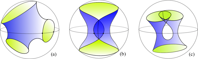
Examples of harmonic maps from surfaces to ${\mathbb{H}}^{3}$, with prescribed boundary values at infinity, such as discussed in this paper.

As we will see later on in Paragraph 2.1, proving Theorem 1.1 amounts to solving a Dirichlet problem at infinity. Recall that a map $h_{\infty}:\SS^{k-1}\to\SS^{n-1}$ ($k,n\geq 2$) is quasi-regular if it is locally the boundary value of some quasi-isometric map from ${\mathbb{H}}^{k}$ to ${\mathbb{H}}^{n}$. The following concrete example is again a special case of our theorem, illustrated in Figure (b).

Corollary 1.3

Let $h_{\infty}:\SS^{k-1}\to\SS^{n-1}$ be a quasi-regular map. Then, $h_{\infty}$ extends as a harmonic map $h:{\mathbb{H}}^{k}\to{\mathbb{H}}^{n}$.

When $k=n$, Corollary 1.3 was proved by Pankka and Souto in [22].

Figure (c) illustrates Theorem 1.1 in a situation that combines those of Corollaries 1.2 and 1.3.

Let us now explain the hypotheses and conclusion of Theorem 1.1. A map $f:X\to Y$ between two metric spaces is quasi-isometric if there exists a constant $c\geq 1$ such that

$$c^{-1\,}d(x,x^{\prime})-c\leq d(f(x),f(x^{\prime}))\leq c\,d(x,x^{\prime})+c$$ (1.1)

holds for any $x,x^{\prime}\in X$. Such a map needs not be continuous.

A smooth map $h:X\to Y$ between Riemannian manifolds is harmonic if it is a critical point for the Dirichlet energy $\int|Dh|^{2}$, namely if it satisfies the elliptic PDE

$${\rm Tr}\,D^{2}h=0\,.$$

A pinched Hadamard manifold is a complete simply-connected Riemannian manifold $X$ with dimension at least 2 whose sectional curvature is pinched between two negative constants, namely

$$-b^{2}\leq K_{X}\leq-a^{2}<0\,.$$ (1.2)

Observe that working with pinched Hadamard manifolds provides a natural and elegant framework to deal simultaneously with all the rank one symmetric spaces.

A discrete subgroup $\Gamma\subset{\rm Is\,}(X)$ is convex cocompact when the convex core $K\subset M$ is compact, see Definition 2.5. We will see in Section 2 (Proposition 2.6) that requiring the discrete subgroup $\Gamma\subset{\rm Is\,}(X)$ to be convex cocompact is equivalent to assuming that the Riemannian quotient $M=\Gamma\backslash X$ is Gromov hyperbolic, and that its injectivity radius ${\rm inj}:M\to[0,\infty[$ is a proper function on $M$. Therefore we can speak of the boundary at infinity $\partial_{\infty}M$ of $M$.

Definition 1.4

A map $f:M\to Y$ is locally quasi-isometric at infinity if it satisfies the two conditions :

(a) the map $f$ is rough Lipschitz : there exists a constant $c\geq 1$ such that $d(f(m),f(p))\leq c\,d(m,p)+c$ for any $p,m\in M$ ;

(b) each point $\xi\in\partial_{\infty}M$ in the boundary at infinity of $M$ admits a neighbourhood $U_{\xi}$ in $M\cup\partial_{\infty}M$ such that the restriction $f:U_{\xi}\cap M\to Y$ is quasi-isometric.

Note that condition (a) follows from condition (b) when the map $f$ is bounded on compact subsets of $M$.

In Section 3, we give a few counter-examples that emphasise the relevance of assuming in Theorem 1.1 that $\Gamma$ is convex cocompact.

Note that the assumption that $\Gamma$ is torsion-free in Theorem 1.1 is only used to ensure that the quotient $M=\Gamma\backslash X$ is a manifold. See Kapovich [15] for nice examples of non torsion-free groups.

1.3 Structure of the proof

Although the rough structure of the proof of Theorem 1.1 is similar to those of [4] or [6], we now have to deal with new issues. Two new crucial steps will be understanding the geometry of the source manifold $M=\Gamma\backslash X$ in Proposition 2.6, and obtaining uniform estimates for the harmonic measures on $M$ in Corollary 6.20.

Let us now give an overview of the proof of existence in Theorem 1.1. We refer to Section 4 for complete proofs of existence and uniqueness.

Replacing the quasi-isometric map $f$ by local averages in Lemma 4.1, we may assume that $f$ is smooth. This averaging process even allows us to assume that $f$ has uniformly bounded first and second covariant derivatives, a fact that will be crucial later on to prove the so-called boundary estimates of Paragraph 4.4.

To prove existence, we begin by solving a family of Dirichlet problems on bounded domains of $M$. Namely, we introduce in Proposition 4.2 an exhausting and increasing family of compact convex domains $V_{R}\subset M$ with smooth boundaries ($R>0$), and consider for each $R>0$ the unique harmonic map $h_{R}:V_{R}\to Y$ which is solution of the Dirichlet problem “$h_{R}=f$ on the boundary $\partial V_{R}$” (Lemma 4.7).

The heart of the proof, in Proposition 4.8, consists in showing that the distances $d(h_{R},f)$ are uniformly bounded by a constant $\bar{\rho}$ that does not depend on $R$. Once we have this bound, we recall in Paragraph 4.3 a standard compactness argument that ensures that the family of harmonic maps $(h_{R})$ converges, when $R$ goes to infinity, to a harmonic map $h:M\to Y$. The limit harmonic map $h$ still satisfies $d(h,f)\leq\bar{\rho}$.

Let us now briefly explain how we obtain this uniform bound for the distances $\rho_{R}:=d(h_{R},f)$. We assume by contradiction that $\rho_{R}$ is very large.

The first step consists in proving that the distance $\rho_{R}$ is achieved at a point $m\in M$ which is far away from the boundary $\partial V_{R}$. This relies on the uniform bound for the covariant derivatives $Df$ and $D^{2}f$, and on the equality $d(h_{R}(p),f(p))=0$ when $p$ lies in the boundary $\partial V_{R}$.

The second step consists in the so-called interior estimates of Section 7. Since the point $m\in V_{R}$ such that $\rho_{R}=d(h_{R}(m),f(m))$ is far away from the boundary $\partial V_{R}$, we may select a large neighbourhood $W(m)\subset M$ of the point $m$, such that $W(m)\subset V_{R}$.

Let us describe the neighbourhoods $W(m)$. We fix two large constants $1\ll\ell_{0}\ll\ell$ that will not depend on $R$ and need to be properly chosen. If $m$ is far enough from the convex core $K\subset M$, the injectivity radius at the point $m$ will be larger than $\ell_{0}$ and we will choose $W(m)$ to be the Riemannian ball $W(m)=B(m,\ell_{0})\subset V_{R}$ with center $m$ and radius $\ell_{0}$. If $m$ is close to the convex core, we will chose $W(m)=V_{\ell}\subset V_{R}$ to be a fixed large compact neighbourhood of the convex core $K$.

To wrap up the proof in Section 7, we will exploit the subharmonicity of the function $q\in W(m)\to d(f(m),h_{R}(q))\in[0,\infty[$. The crucial tool for obtaining a contradiction, and thus proving that $\rho_{R}$ cannot be very large, is uniform estimates for the harmonic measures of the boundaries of these neighbourhoods $W(m)$ relative to the point $m$ that are proved in Sections 5 and 6. See Proposition 5.2 and Corollary 6.20. We refer to Paragraph 7.3 for a more precise overview of this part the proof.

2 Convex cocompact subgroups of ${\rm Is\,}(X)$

In this section we characterize convex cocompact subgroups $\Gamma\subset{\rm Is\,}(X)$ in terms of the geometric properties of the quotient $\Gamma\backslash X$.

2.1 Gromov hyperbolic metric spaces

We first recall a few facts and definitions concerning Gromov hyperbolic metric spaces, see [12].

Let $\delta>0$. A geodesic metric space $X$ is said to be $\delta$-Gromov hyperbolic when every geodesic triangle $\Delta$ in $X$ is $\delta$-thin, namely when each edge of $\Delta$ lies in the $\delta$-neighbourhood of the union of the other two edges. For example, any pinched Hadamard manifold is Gromov hyperbolic for some constant $\delta_{X}$ that depends only on the upper bound for the curvature.

When the Gromov hyperbolic space $X$ is proper, namely its balls are compact, the boundary at infinity $\partial_{\infty}X$ of $X$ may be defined as the set of equivalence classes of geodesic rays, where two geodesic rays are identified when they remain within bounded distance from each other. In case $X$ is a pinched Hadamard manifold, the boundary at infinity (or visual boundary) $\partial_{\infty}X$ naturally identifies with the tangent sphere at any point $x\in X$. The boundary at infinity provides a compactification $\overline{X}=X\cup\partial_{\infty}X$ of $X$.

A quasi-isometric map $f:X\to Y$ between proper Gromov hyperbolic spaces admits a boundary value $\partial_{\infty}f:\partial_{\infty}X\to\partial_{\infty}Y$, and two quasi-isometric maps $f_{1},f_{2}:X\to Y$ have the same boundary value if and only if $d(f_{1},f_{2})<\infty$.

Since our quotient $M=\Gamma\backslash X$ is Gromov hyperbolic (see Proposition 2.6), we may thus rephrase the conclusion of Theorem 1.1 in case $f$ is assumed to be globally quasi-isometric.

Corollary 2.1

Given a quasi-isometric map $f:M\to Y$, there exists a unique harmonic quasi-isometric map $h:M\to Y$ which is a solution to the Dirichlet problem at infinity with boundary value

$$\partial_{\infty}h=\partial_{\infty}f:\partial_{\infty}M\to\partial_{\infty}Y\,.$$

2.2 Gromov product

In Section 7, we shall use Gromov products in the Gromov hyperbolic manifolds $M$ and $Y$ to carry out the proof of Theorem 1.1. Here, we recall the definition and two properties of the Gromov product.

In a metric space, the Gromov product of the three points $x,x_{1},x_{2}$ is defined as

$$(x_{1},x_{2})_{x}=\frac{1}{2}(d(x,x_{1})+d(x,x_{2})-d(x_{1},x_{2}))\,.$$

Gromov hyperbolicity may be expressed in terms of Gromov products. Also, in a Gromov hyperbolic space, the Gromov product $(x_{1},x_{2})_{x}$ is roughly equal to the distance from $x$ to a minimizing geodesic segment $[x_{1},x_{2}]$. In particular, the following holds.

Lemma 2.2

[12, Chap.2] Let $X$ be a $\delta$-Gromov hyperbolic space. Then, for any points $x,x_{1},x_{2},x_{3}\in X$ and any minimizing geodesic segment $[x_{1},x_{2}]\subset X$, one has

$$(x_{1},x_{3})_{x} \geq\min((x_{1},x_{2})_{x},(x_{2},x_{3})_{x})-2\delta$$ (2.1)

$$(x_{1},x_{2})_{x} \leq d(x,[x_{1},x_{2}])\leq(x_{1},x_{2})_{x}+2\delta\ .$$ (2.2)

Moreover, the next lemma tells us that Gromov products are quasi-invariant under quasi-isometric maps.

Lemma 2.3

[12, Prop.5.15] Let $X$ and $Y$ be Gromov hyperbolic spaces, and $f:X\to Y$ be a $c$ quasi-isometric map. Then, there exists a constant $A>0$ such that, for any three points $x,x_{1},x_{2}\in X$ :

$$c^{-1}\,(x_{1},x_{2})_{x}-A\leq(f(x_{1}),f(x_{2}))_{f(x)}\leq c\,(x_{1},x_{2})_{x}+A\,.$$

2.3 Convex cocompact subgroups

We begin with definitions that are classical in the hyperbolic space ${\mathbb{H}}^{k}$. See Bowditch [8] for a reference dealing with pinched Hadamard manifolds.

Definition 2.4

Let $X$ be a pinched Hadamard manifold and $\Gamma\subset{\rm Is\,}(X)$ be a discrete subgroup of the group of isometries of $X$.

The limit set $\Lambda_{\Gamma}\subset\partial_{\infty}X$ of the group $\Gamma$ is the closed subset of $\partial_{\infty}X$ defined as $\Lambda_{\Gamma}=\overline{\Gamma x}\smallsetminus\Gamma x$, where $x$ is any point in $X$ and the closure $\overline{\Gamma x}$ of its orbit is taken in the compactification $\overline{X}=X\cup\partial_{\infty}X$.

The domain of discontinuity of $\Gamma$ is $\Omega_{\Gamma}=\partial_{\infty}X\smallsetminus\Lambda_{\Gamma}$. It is an open subset of the boundary at infinity $\partial_{\infty}X$. The group $\Gamma$ acts properly discontinuously on $X\cup\Omega_{\Gamma}\subset\overline{X}$.

Recall that a subset $C\subset M$ of a Riemannian manifold is geodesically convex if, given two points $m_{1},m_{2}\in C$, any minimizing geodesic segment $[m_{1},m_{2}]$ joining these two points lies in $C$.

Definition 2.5

Let $X$ be a pinched Hadamard manifold, $\Gamma\subset{\rm Is\,}(X)$ be an infinite discrete subgroup of the isometry group of $X$ and $M=\Gamma\backslash X$.

The convex hull ${\rm conv}\Lambda_{\Gamma}\subset X$ of $\Lambda_{\Gamma}$ is the smallest closed geodesically convex subset $C$ of $X$ such that $\overline{C}\smallsetminus C=\Lambda_{\Gamma}$ (where the closure $\overline{C}$ is again taken in the compactification $\overline{X}$). The convex core of $M$ is the quotient $K:=\Gamma\backslash({\rm conv}\Lambda_{\Gamma})\subset M$.

The group $\Gamma$ is said to be convex cocompact if the convex core $K\subset M$ is compact. This is equivalent to requiring the quotient $\Gamma\backslash(X\cup\Omega_{\Gamma})\subset\Gamma\backslash\overline{X}$ to be compact. See [8, Th.6.1].

The hypothesis in Theorem 1.1 that $\Gamma$ is convex cocompact will be used in this paper through the following characterization in terms of geometric properties of the Riemannian quotient $M$.

Proposition 2.6

Let $X$ be a pinched Hadamard manifold and $\Gamma\subset{\rm Is\,}(X)$ be an infinite torsion-free discrete subgroup. Then, the group $\Gamma$ is convex cocompact if and only if $M=\Gamma\backslash X$ satisfies the following conditions :

• the quotient $M$ is Gromov hyperbolic ;

• the injectivity radius ${\rm inj}:M\to[0,\infty[$ is a proper function.

Proposition 2.6 is proved in Paragraphs 2.4, 2.5 and 2.6 below.

2.4 Gromov hyperbolicity of the quotient $M=\Gamma\backslash X$

In this paragraph, $X$ is our pinched Hadamard manifold, $\Gamma\subset{\rm Is\,}(X)$ is a torsion-free convex cocompact subgroup and $M=\Gamma\backslash X$. We want to prove that there exists a constant $\delta>0$ such that every triangle $T\subset M$ in the quotient is $\delta$-thin. To do this, we start with quadrilaterals. We first recall a result by Reshetnyak that compares quadrilaterals in a Hadamard manifold with quadrilaterals in the model hyperbolic plane ${\mathbb{H}}^{2}(-a^{2})$ with constant curvature $-a^{2}$.

Lemma 2.7

Reshetnyak comparison lemma [23]

Let $X$ be a Hadamard manifold satisfying the pinching assumption (1.2). For every quadrilateral $[x,y,z,t]$ in $X$, there exists a convex quadrilateral $[\bar{x},\bar{y},\bar{z},\bar{t}]$ in ${\mathbb{H}}^{2}(-a^{2})$ and a map $j:[\bar{x},\bar{y},\bar{z},\bar{t}]\to X$ that is $1$-Lipschitz, that sends respectively the vertices $\bar{x},\bar{y},\bar{z},\bar{t}$ on $x,y,z,t$, and whose restriction to each one of the four edges of $[\bar{x},\bar{y},\bar{z},\bar{t}]$ is isometric.

We now deduce from the Reshetnyak Lemma a standard property of quadrilaterals in $X$, that will be used again in the proof of Proposition 6.16. The Gromov hyperbolicity of $X$ ensures that any edge of a quadrilateral in $X$ lies in the $2\delta_{X}$-neighbourhood of the union of the three other edges. One can say more under an angle condition. Namely :

Lemma 2.8

Thin quadrilaterals in $X$
Let $X$ be a pinched Hadamard manifold. Let $\varepsilon>0$. There exists an angle $0<\alpha_{\varepsilon}<\pi/2$ and a distance $\tilde{\delta}_{\varepsilon}$ such that for any quadrilateral $[x,x_{1},y_{1},y]$ in the Hadamard manifold $X$ with $d(x_{1},y_{1})\geq\varepsilon$, and whose angles at both vertices $x_{1}$ and $y_{1}$ satisfy $\angle_{x_{1}}\geq\pi/2-\alpha_{\varepsilon}$ and $\angle_{y_{1}}\geq\pi/2-\alpha_{\varepsilon}$, the $\tilde{\delta}_{\varepsilon}$-neighbourhood of the edge $[x,y]$ contains the union of the other three edges, namely :

$$[x,x_{1}]\cup[x_{1},y_{1}]\cup[y_{1},y]\subset{\cal V}_{\tilde{\delta}_{\varepsilon}}([x,y])\,.$$

Proof  When $X$ is the hyperbolic plane, the easy proof is left to the reader. The general case follows from this special case and the Reshetnyak comparison lemma 2.7. Indeed, the comparison quadrilateral also satisfies the distance and angles conditions at the points $\bar{x}_{1}$ and $\bar{y}_{1}$. $\Box$

We now turn to quadrilaterals in our quotient space $M=\Gamma\backslash X$. In the whole paper, unless otherwise specified, all triangles and quadrilaterals in $M$ will be assumed to be minimizing, namely their edges will be minimizing geodesic segments.

Lemma 2.9

Thin quadrilaterals in $M$

Assume that $X$ is a pinched Hadamard manifold, that $\Gamma\subset{\rm Is\,}(X)$ is a torsion-free convex cocompact subgroup, and let $M=\Gamma\backslash X$. Let $V\subset M$ be a compact convex subset of $M$ whose lift $\tilde{V}\subset X$ is convex.

(1) There exists $\delta_{0}$ such that, for any quadrilateral $[p,p_{1},q_{1},q]$ in $M$ with both $p_{1},q_{1}\in V$, any edge of this quadrilateral lies in the $\delta_{0}$-neighbourhood of the union of the three other edges.

(2) Let $\varepsilon>0$. There exists $\delta_{\varepsilon}$ such that if we assume moreover that $p_{1},q_{1}\in V$ are respectively the projections of the points $p$ and $q$ on the convex set $V$, and that $d(p_{1},q_{1})\geq\varepsilon$, then :

$$[p,p_{1}]\cup[p_{1},q_{1}]\cup[q_{1},q]\subset{\cal V}_{\delta_{\varepsilon}}([p,q])\,.$$

Proof  Lift successively the minimizing geodesic segments $(p_{1}p)$, $(pq)$ and $(qq_{1})$ to geodesic segments $(x_{1}x)$, $(xy)$ and $(yy_{1})$ in $X$, so that the geodesic segment $(x_{1}y_{1})$ projects to a curve $c$ from $p_{1}$ to $q_{1}$ that lies in $V$.

Since both the curve $c$ and the geodesic segment lie in the compact set $V$, the conclusion follows from Lemma 2.8, with $\delta_{0}=2\delta_{X}+d_{V}$ and $\delta_{\varepsilon}=\tilde{\delta}_{\varepsilon}+d_{V}$, where $d_{V}$ denotes the diameter of $V$. $\Box$

Corollary 2.10

Gromov hyperbolicity of the quotient $\Gamma\backslash X$

Assume that $X$ is a pinched Hadamard manifold and that $\Gamma\subset{\rm Is\,}(X)$ is a torsion-free convex cocompact subgroup. Then, the quotient $M=\Gamma\backslash X$ is Gromov hyperbolic.

Proof  Let $V\subset M$ be a compact convex neighbourhood of the convex core with smooth boundary, whose lift in $X$ is convex. Such a neighbourhood will be constructed in Proposition 4.2. Let $\varepsilon={\rm inj}(V)/2$ (where ${\rm inj}(V)=\inf_{m\in V}{\rm inj}(m)$ denotes the injectivity radius on $V$).

Let $T=[p,q,r]$ be a triangle in $M$. In case where at least one of the vertices of $T$ lies in $V$, Lemma 2.9 applied to a quadrilateral with two equal vertices proves that $T$ is $\delta_{0}$-thin.

We now turn to the case where none of $p,q,r$ lie in $V$ and denote by $p_{1},q_{1},r_{1}$ their projections on $V$.

Assume first that $d(p_{1},q_{1})\leq\varepsilon$ and $d(q_{1},r_{1})\leq\varepsilon$. Then, the triangle $[p_{1},q_{1},r_{1}]$ is homotopically trivial. Writing $p={\rm exp}_{p_{1}}u$ with $u$ a normal vector to $V$ at point $p_{1}$ (and similarly for $q$ and $r$) we construct an homotopy between $[p,q,r]$ and a constant map, so that the triangle $[p,q,r]$ lifts to a triangle $[x,y,z]$ in $X$. Since $X$ is $\delta_{X}$-Gromov hyperbolic, $[x,y,z]$ is $\delta_{X}$-thin, hence $[p,q,r]$ is $\delta_{X}$-thin too.

Assume now that $d(p_{1},q_{1})\geq\varepsilon$ and $d(q_{1},r_{1})\geq\varepsilon$. The first part of Lemma 2.9, applied to the quadrilateral $[p,p_{1},r_{1},r]$, yields that $[p,r]$ lies in the $\delta_{0}$-neighbourhood of $[p,p_{1}]\cup[p_{1},r_{1}]\cup[r_{1},r]$, so that $[p,r]$ lies in the $(\delta_{0}+d_{V})$-neighbourhood of $[p,p_{1}]\cup[r_{1},r]$ (recall that $d_{V}$ is the diameter of $V$). The second part of Lemma 2.9 now applied to both quadrilaterals $[p,p_{1},q_{1},q]$ and $[q,q_{1},r_{1},r]$ yields that $[p,r]$ lies in the $(\delta_{0}+\delta_{\varepsilon}+d_{V})$-neighbourhood of $[p,q]\cup[q,r]$.

Assume finally that $d(p_{1},q_{1})\leq\varepsilon$ and $d(q_{1},r_{1})\geq\varepsilon$. It follows from the first part of Lemma 2.9 that $[p,r]$ lies in the $(\delta_{0}+d_{V})$-neighbourhood of $[p,p_{1}]\cup[r_{1},r]$ and that $[p,p_{1}]$ lies in the $(\delta_{0}+d_{V})$-neighbourhood of $[p,q]\cup[q_{1},q]$, while the second part of this Lemma ensures that $[q,q_{1}]\cup[r_{1},r]$ lies in the $\delta_{\varepsilon}$-neighbourhood of $[q,r]$.

Hence, every triangle in $M$ is $(2(\delta_{0}+d_{V})+\delta_{\varepsilon}+\delta_{X})$-thin, so that $M$ is Gromov hyperbolic. $\Box$

2.5 Injectivity radius of the quotient $M=\Gamma\backslash X$

Our aim in this paragraph is the following.

Proposition 2.11

Properness of the injectivity radius

Assume that $X$ is a pinched Hadamard manifold and that $\Gamma\subset{\rm Is\,}(X)$ is a torsion-free convex cocompact subgroup. Let $M=\Gamma\backslash X$.

Then, the injectivity radius ${\rm inj}:M\to[0,\infty[$ is a proper function.

Proof  For $p\in M$, we denote by $i(p)$ the injectivity radius at the point $p$, and let $j(p)=\inf\{d(\tilde{p},\gamma\tilde{p})\,|\,\gamma\in\Gamma^{*}\}$, where $\tilde{p}\in X$ is a lift of $p$ and $\Gamma^{*}$ is the set of non trivial elements in $\Gamma$. Since $M$ has non positive curvature, there are no conjugate points in $M$ hence $j(p)=2i(p)$.

We proceed by contradiction and assume that there exists a sequence $(p_{n})$ of points in $M$ going to infinity, and such that the injectivity radii $i(p_{n})$ remain bounded. Let $q_{n}$ denote the projection of the point $p_{n}$ on the convex core $K\subset M$ ($n\in{\mathbb{N}}$). Since $\Gamma$ is convex cocompact, there exists a compact $L\subset X$ such that each $q_{n}$ lifts in $X$ to a point $\tilde{q}_{n}\in L$. Then, the geodesic segment $[q_{n},p_{n}]$ lifts as $[\tilde{q}_{n},\tilde{p}_{n}]$. By hypothesis, there exists $I>0$ and a sequence $\gamma_{n}\in\Gamma^{*}$ such that $d(\tilde{p}_{n},\gamma_{n}\tilde{p}_{n})\leq I$. Since the projection $X\to{\rm conv}(\Lambda_{\Gamma})$ commutes to the action of $\Gamma$ and is $1$-Lipschitz, it follows that $d(\tilde{q}_{n},\gamma_{n}\tilde{q}_{n})\leq I$. By compactness of $L$, and since $\Gamma$ is discrete, one may thus assume that the sequence $(\tilde{q}_{n})$ converges to a point $\tilde{q}\in L$ and that the bounded sequence $(\gamma_{n})$ is constant, equal to $\gamma\in\Gamma^{*}$. The boundary at infinity $\partial_{\infty}X$ being compact, we may also assume that the sequence of geodesic rays $([\tilde{q}_{n},\tilde{p}_{n}\mathclose{[})$ converges to a geodesic ray $[\tilde{q},\xi\mathclose{[}$ where $\xi\in\partial_{\infty}X$.

By construction, the geodesic ray $[\tilde{q},\xi\mathclose{[}$ is within bounded distance $I$ from its image $[\gamma\tilde{q},\gamma\xi\mathclose{[}$, hence $\xi\in\partial_{\infty}X$ is a fixed point of $\gamma$. The group $\Gamma$ being discrete and torsion-free, it has no elliptic elements, so that $\xi\in\Lambda_{\Gamma}$. Thus, the whole geodesic ray $[\tilde{q},\xi\mathclose{[}$ lies in ${\rm conv}(\Lambda_{\Gamma})$, a contradiction to the fact that the sequence $(p_{n})$ goes to infinity in $M$. $\Box$

2.6 Converse

In this paragraph, we complete the proof of Proposition 2.6 by proving the following.

Proposition 2.12

Let $X$ be a pinched Hadamard manifold, and $\Gamma\subset{\rm Is\,}(X)$ be a torsion-free discrete subgroup. Assume that the quotient manifold $M=\Gamma\backslash X$ is Gromov hyperbolic, and that the injectivity radius ${\rm inj}:M\to[0,\infty[$ is a proper function.

Then, the group $\Gamma$ is convex cocompact.

We want to prove that the convex core $K:=\Gamma\backslash({\rm conv}\Lambda_{\Gamma})$ is a compact subset of $M$, where ${\rm conv}\Lambda_{\Gamma}$ denotes the convex hull of the limit set of $\Gamma$. We will rather work with the join of the radial limit set $\Lambda_{\Gamma}^{r}$.

Definition 2.13

A geodesic ray $c:[0,\infty[\to M$ is said to be recurrent when it is not a proper map, that is if there exists a sequence $t_{n}\to+\infty$ and a compact set $L_{c}\subset M$ (that might depend on $c$) with $c(t_{n})\in L_{c}$.

The radial limit set $\Lambda_{\Gamma}^{r}\subset\Lambda_{\Gamma}$ of $\Gamma$ is the set of endpoints $\xi\in\partial_{\infty}X$ of geodesic rays in $X$ that project to a recurrent geodesic ray in $M$.

Since there exist closed geodesics in the negatively curved manifold $M$, the radial limit set $\Lambda_{\Gamma}^{r}$ is not empty, and it is a $\Gamma$-invariant subset of $\partial_{\infty}X$. Hence, the limit set $\Lambda_{\Gamma}$ being a minimal $\Gamma$-invariant closed subset of $\partial_{\infty}X$, it follows that $\Lambda_{\Gamma}^{r}$ is dense in $\Lambda_{\Gamma}$.

Definition 2.14

The join of a closed subset $Q\subset\partial_{\infty}X$ is defined as

$${\rm join}\,Q=\bigcup_{\xi_{1},\xi_{2}\in Q}\mathopen{]}\xi_{1},\xi_{2}\mathclose{[}\subset X\,$$

where $\mathopen{]}\xi_{1},\xi_{2}\mathclose{[}$ denotes the geodesic line with endpoints $\xi_{1}$ and $\xi_{2}$.

The join is thus the first step towards the construction of the convex hull. One has ${\rm join}\,Q\subset{\rm conv}Q$. The following result by Bowditch [8] investigates how much we miss in the convex hull by considering only the join.

Proposition 2.15

[8, Lemma 2.2.1 and Proposition 2.5.4]

Let $X$ be a pinched Hadamard manifold. There exists a real number $\lambda>0$ that depends only on the pinching constants such that, for any closed subset $Q\subset\partial_{\infty}X$, the convex hull of $Q$ lies in the $\lambda$-neighbourhood of the join of $Q$.

Let us now proceed with our proof. The projection $K^{r}_{j}:=\Gamma\backslash({\rm join}\,\Lambda_{\Gamma}^{r})\subset M$ of the join of the radial limit set is the union of all the recurrent geodesics on $M$, namely of all geodesics that are recurrent both in the future and in the past. We begin with the following.

Proposition 2.16

Under the assumptions of Proposition 2.12, the join of the radial limit set of $\Gamma$ projects in $M$ to a bounded set $K^{r}_{j}$.

Proof  Proposition 2.16 is an immediate consequence of the definition of the join and of Lemma 2.18 below. $\Box$

For $r>0$, define $M_{r}=\{m\in M\,|\;{\rm inj}(m)\leq r\}$. Under our hypotheses, $M_{r}$ is a compact subset of $M$. Let $\delta>0$ such that $M$ is $\delta$-Gromov hyperbolic.

Lemma 2.17

Any geodesic segment in $M$ whose image lies outside the compact subset $M_{3\delta}\subset M$ is minimizing.

Proof  We proceed by contradiction and assume that the geodesic segment $c:[0,l]\to M\smallsetminus M_{3\delta}$ is minimizing, but ceases to be minimizing on any larger interval. Since $M$ has negative curvature, there are no conjugate points, so that there exists another minimizing geodesic $\bar{c}:[0,l]\to M$ with the same endpoints $c_{0}$ and $c_{l}$ as $c$.

The manifold $M$ being $\delta$-hyperbolic, the geodesic segments $c$ and $\bar{c}$ are within distance $\delta$ from each other. We may thus choose a subdivision $(x_{p})_{0\leq p\leq P}$ of $c([0,l])$ with $x_{0}=c_{0}$, $x_{P}=c_{l}$, and such that $d(x_{p},x_{p+1})\leq\delta$ when $0\leq p<P$, and another sequence $(y_{p})_{0\leq p\leq P}$ with $y_{p}\in\bar{c}([0,l])$ and $d(x_{p},y_{p})\leq\delta$ when $0\leq p\leq P$. In particular, $d(y_{p},y_{p+1})\leq 3\delta$, so that the length of any of the quadrilaterals $q_{p}=[x_{p},x_{p+1},y_{p+1},y_{p}]$ is at most $6\delta$. Since the injectivity radius at the point $x_{p}$ is larger than $3\delta$, it follows that each quadrilateral $q_{p}$ is homotopically trivial, so that $c([0,l])$ and $\bar{c}([0,l])$ themselves are homotopic. But $X$ being a Hadamard manifold then yields $c=\bar{c}$, which is a contradiction. $\Box$

Lemma 2.18

Let $d_{3\delta}$ denote the diameter of $M_{3\delta}$. Under the assumption of Proposition 2.12, any recurrent geodesic in $M$ lies in a fixed compact subset of $M$. More precisely, such a geodesic lies in the $d_{3\delta}$-neighbourhood of $M_{3\delta}$.

Proof  Let $c:{\mathbb{R}}\to M$ be a geodesic that lifts to a geodesic $\tilde{c}:{\mathbb{R}}\to X$ with both endpoints in $\Lambda^{r}_{\Gamma}$.

We first claim that both geodesic rays $c_{|[0,\infty[}$ and $c_{|]-\infty,0]}$ must keep visiting $M_{3\delta}$. If this were not the case, Lemma 2.17 would ensure that one of these geodesic rays would be eventually minimizing, thus contradicting the assumptions that both endpoints of $c$ lie in the radial limit set.

Now assume by contradiction that the image of $c$ does not lie in the $d_{3\delta}$-neighbourhood of $M_{3\delta}$. Then we can find an interval $[a,b]$ such that $c(a),c(b)\in M_{3\delta}$ but with $c(t)\notin M_{3\delta}$ for every $t\in]a,b[$, and such that $c([a,b])$ exits the $d_{3\delta}$-neighbourhood of $M_{3\delta}$. Hence this geodesic segment $c([a,b])$ has length at least $2d_{3\delta}$. By Lemma 2.17 it would be minimizing, a contradiction to the fact that $d(c(a),c(b))\leq d_{3\delta}$. $\Box$

Proof of Proposition 2.12 We noticed earlier that the radial limit set $\Lambda^{r}_{\Gamma}\subset\Lambda_{\Gamma}$ is dense in the limit set of $\Gamma$. Thus, the join of the full limit set lies in the closure of the join of the radial limit set. Hence Proposition 2.16 ensures that ${\rm join}\,\Lambda_{\Gamma}$ projects to a bounded subset of $M$.

Now Proposition 2.15 ensures that ${\rm conv}\Lambda_{\Gamma}$ also projects to a bounded subset of $M$ or, in other words, that the group $\Gamma$ is convex cocompact. $\Box$

3 Examples

Before going into the proof of Theorem 1.1, we proceed with a few examples and counter-examples.

3.1 Two examples on the annulus

We begin with a family of straightforward applications of Theorem 1.1.

Let ${\mathbb{A}}(r)=\{z\in{\mathbb{C}}\,|\;1/r<|z|<r\}$ and ${\mathbb{D}}=\{z\in{\mathbb{C}}\,|\;|z|<1\}$ be an annulus ($r>1$) or the disk equipped with their complete hyperbolic metrics.

Example 3.1

For every $\alpha\in{\mathbb{R}}$, there exists a unique harmonic quasi-isometric map $h_{\alpha}:{\mathbb{A}}(r)\to{\mathbb{D}}$ with boundary value $g_{\alpha}:\partial_{\infty}({\mathbb{A}}(r))\to\partial_{\infty}{\mathbb{D}}$ defined as

$$g_{\alpha}(re^{i\theta})=e^{i\theta}\qquad g_{\alpha}(e^{i\theta}/r)=e^{i(\theta+\alpha)}\,.$$

Note that the case where the parameter $\alpha$ is equal to $0$ is rather easy. Indeed, the uniqueness of the harmonic map with boundary value $g_{0}$ ensures that $h_{0}$ has a symmetry of revolution and thus reads as $h_{0}(te^{i\theta})=u(t)e^{i\theta}$, and the condition that $h_{0}$ is harmonic reduces to a second order ordinary differential equation on $u$ whose solutions can be expressed in terms of elliptic integrals.

We now give an illustration of Theorem 1.1 where the restriction of the boundary map to each connected component of the boundary at infinity $\partial_{\infty}M$ is not injective.

Example 3.2

The map $g:\partial_{\infty}({\mathbb{A}}(r))\to\partial_{\infty}{\mathbb{D}}$ defined as

$$g(re^{i\theta})=e^{2i\theta}\qquad g_{\alpha}(e^{i\theta}/r)=e^{-3i\theta}$$

is the boundary value of a harmonic map $h:{\mathbb{A}}(r)\to{\mathbb{D}}$.

3.2 First counter-example : surfaces admitting a cusp

In the next two paragraphs, we provide counter-examples to emphasize the importance of assuming that $\Gamma$ is convex cocompact.

We first prove non-existence for hyperbolic surfaces with a cusp.

Proposition 3.3

Let $S$ be a non compact hyperbolic surface of finite topological type admitting at least one cusp, and $Y$ be a pinched Hadamard manifold. Then, there exists no harmonic quasi-isometric map $h:S\to Y$.

Note that, such a surface $S$ being quasi-isometric to the wedge of a finite number of hyperbolic disks and rays, there always exist quasi-isometric maps $f:S\to{\mathbb{H}}^{n}$ for any $n\geq 3$ – none of them harmonic. This proposition is an immediate consequence of the following lemma.

Lemma 3.4

Let $\tau>0$ and $\Sigma$ be the quotient of $\{z\in{\mathbb{C}}\,|\;{\rm Im}z\geq 1\}$, equipped with the hyperbolic metric $\frac{|dz|^{2}}{({\rm Im\,}z)^{2}}$ under the map $z\to z+\tau$.

Let $Y$ be a pinched Hadamard manifold. Then, there is no harmonic quasi-isometric map $h:\Sigma\to Y$.

To prove lemma 3.4, we will use the following result, which will also be crucial for the proof of uniqueness in Theorem 1.1.

Lemma 3.5

[6, Lemma 5.16] Let $M$, $Y$ be Riemannian manifolds, and assume that $Y$ has non positive curvature. Let $h_{0},h_{1}:M\to Y$ be harmonic maps. Then, the distance function $m\in M\to d(h_{0}(m),h_{1}(m))\in{\mathbb{R}}$ is subharmonic.

Proof of Lemma 3.4 Assuming that there exists a harmonic quasi-isometric map $h:\Sigma\to Y$, we will prove that $h$ takes its values in a bounded domain of $Y$. This is a contradiction since $\Sigma$ is unbounded.

Let ${\cal H}_{t}=\{{\rm Im}\,z=e^{t}\}/{<\tau>}\subset\Sigma$ denote the horocyle at distance $t\geq 0$ from ${\cal H}_{0}$. Pick a point $z_{0}\in{\cal H}_{0}$ and let $m_{0}=h(z_{0})\in Y$. Since $h$ is harmonic, Lemma 3.5 ensures that the function $\varphi:z\in\Sigma\to d(h(z),m_{0})\in[0,\infty[$ is subharmonic. Since $h$ is quasi-isometric, there exists a constant $k>0$ such that $\varphi(z)\leq k(t+1)$ for any $z\in{\cal H}_{t}$, with $t\geq 0$.

Let now $T>0$ and introduce the harmonic function defined on $\Sigma$ by

$$\eta_{T}(z)=k+k(T+1)\,e^{-T}\,{\rm Im\,}z\,.$$

By construction, $\varphi\leq\eta_{T}$ on ${\cal H}_{0}\cup{\cal H}_{T}$, hence the maximum principle ensures that $\varphi(z)\leq\eta_{T}(z)$ holds for any $z\in{\cal H}_{t}$ with $0\leq t\leq T$. In other words, $d(h(z),m_{0})\leq k+k(T+1)\,e^{-T}\,{\rm Im\,}z$ if $T\geq{\rm Im\,}z$. Letting $T\to\infty$ proves that $h$ takes its values in the ball $B(m_{0},k)$, a contradiction since $h$ is quasi-isometric. $\Box$

3.3 A second counterexample

We now give another counter-example where the surface has no cusp, that is when $\Gamma$ has no parabolic element.

Let $\Sigma$ now denote a compact hyperbolic surface whose boundary is the union of two totally geodesic curves of the same length. We consider a non compact hyperbolic surface $S$ obtained by gluing together infinitely many copies of $\Sigma$ along their boundaries, in such a way that $S$ admits a natural action $\tau$ of ${\mathbb{Z}}$ “by translation”. The quotient $S/\tau$ is then a compact Riemann surface without boundary. Observe that $S$, being quasi-isometric to ${\mathbb{R}}$, is Gromov hyperbolic and that the injectivity radius of $S$ is bounded below but is not a proper function on $S$.

Our aim is to prove the following.

Proposition 3.6

There exist quasi-isometric functions $\varphi:S\to{\mathbb{R}}$ that are not within bounded distance from any harmonic function.

Thus, there exist quasi-isometric maps $f:S\to{\mathbb{H}}^{2}$ that are not within bounded distance from any harmonic map.

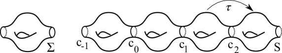
The surface $S$

We will first describe all quasi-isometric harmonic functions on $S$. By applying the afore mentionned theorem by Eeels and Sampson [11] to maps $S/\tau\to{\mathbb{R}}/{\mathbb{Z}}$ between these compact manifolds, we construct a harmonic function $\eta_{1}:S\to{\mathbb{R}}$ that satisfies the relation $\eta_{1}(\tau m)=\eta_{1}(m)+1$ for any point $m\in S$. We may think of the function $\eta_{1}$ as a projection from $S$ onto ${\mathbb{R}}$. It is a quasi-isometric map.

Lemma 3.7

Let $\eta:S\to{\mathbb{R}}$ be a quasi-isometric harmonic function. Then, there exist constants $\alpha\in{\mathbb{R}}^{*}$ and $\beta\in{\mathbb{R}}$ such that $\eta=\alpha\eta_{1}+\beta$.

Proof  We denote by $(c_{n})_{n\in{\mathbb{Z}}}$ the memories in $S$ of the boundary of $\Sigma$, with $c_{n}=\tau^{n}c_{0}$ ($n\in{\mathbb{Z}}$). All these curves have the same finite length.

By adding a suitable constant to $\eta_{1}$, we may assume that $\eta_{1}$ vanishes at some point $m_{0}\in c_{0}$. Let $m_{n}=\tau^{n}(m_{0})\in c_{n}$ so that $\eta_{1}(m_{n})=n$ for $n\in{\mathbb{Z}}$.

Let $t_{n}=\eta(m_{n})$ ($n\in{\mathbb{Z}}$). Replacing the quasi-isometric function $\eta$ by $-\eta$ if necessary, we may assume that $t_{\pm n}\to\pm\infty$ when $n\to+\infty$. Better, there exist a constant $k>1$ and an integer $N\in{\mathbb{N}}$ such that

$$\begin{gathered}\hbox{$|\eta_{1}-n|\leq k$ and $|\eta-t_{n}|\leq k$}\quad\hbox{on $c_{n}$ for $n\in{\mathbb{Z}}$,}\\ \hbox{where $n/k\leq\varepsilon t_{\varepsilon n}\leq kn$ for $\varepsilon=\pm 1$ and $n\geq N$.}\end{gathered}$$

For any $n\geq 1$, let $(\alpha_{n},\beta_{n})\in{\mathbb{R}}^{2}$ be the solution of the linear system

$$-n\alpha_{n}+\beta_{n}=t_{-n}\quad\hbox{and}\quad n\alpha_{n}+\beta_{n}=t_{n}\,.$$

The sequence $(\alpha_{n})$ is bounded since $|\alpha_{n}|\leq k$ when $n\geq N$. The harmonic function $\eta-(\alpha_{n}\eta_{1}+\beta_{n})$ vanishes at both points $m_{n}\in c_{n}$ and $m_{-n}\in c_{-n}$, so that $|\eta-(\alpha_{n}\eta_{1}+\beta_{n})|\leq k(k+1)$ on $c_{n}\cup c_{-n}$ if $n\geq N$. By the maximum principle, it follows that $|\eta-(\alpha_{n}\eta_{1}+\beta_{n})|\leq k(k+1)$ on the compact subset of $S$ cut out by $c_{n}\cup c_{-n}$. By applying this estimate at the point $m_{0}$, we obtain that the sequence $(\beta_{n})$ is also bounded. By going to a subsequence, we may thus assume that $\alpha_{n}\to\alpha$ and $\beta_{n}\to\beta$ when $n\to\infty$, so that the limit harmonic function $\eta-(\alpha\eta_{1}+\beta):S\to{\mathbb{R}}$ is bounded. Since $S$ is a nilpotent cover of a compact Riemannian manifold, a theorem by Lyons-Sullivan [19, Th.1] ensures that this bounded harmonic function is constant. $\Box$

Proof of Proposition 3.6   Let $\varphi:S\to{\mathbb{R}}$ be a quasi-isometric function such that

– $\varphi(m_{n})=n$ when $n=\pm 4^{2p}$

– $\varphi(m_{n})=2n$ when $n=\pm 4^{2p+1}$.

This function $\varphi$ is quasi-isometric, but is not within bounded distance from any function $\alpha\eta_{1}+\beta$.

We now embed isometrically the real line in the hyperbolic plane as a geodesic $\gamma:{\mathbb{R}}\to{\mathbb{H}}^{2}$ and define $f=\gamma\circ\varphi:S\to{\mathbb{H}}^{2}$. Then $f$ is a quasi-isometric map. Assume by contradiction that there exists a harmonic map $h_{1}:S\to{\mathbb{H}}^{2}$ within bounded distance from $f$. Let $h_{2}=\sigma\circ h_{1}:S\to{\mathbb{H}}^{2}$, where $\sigma:{\mathbb{H}}^{2}\to{\mathbb{H}}^{2}$ is the symmetry with respect to geodesic $\gamma$. By Lemma 3.5, the bounded function $t\in S\to d(h_{1}(t),h_{2}(t))\in[0,\infty[$ is subharmonic. Since $S$ is a ${\mathbb{Z}}$-cover of a compact Riemannian manifold, another theorem by Lyons-Sullivan [19, Th.4] ensures that this bounded subharmonic function is constant. Therefore, the harmonic map $h_{1}$ takes its values in a curve which is equidistant to $\gamma$, hence in $\gamma$. This means that $h_{1}$ reads as $h_{1}=\gamma\circ\eta$ with $\eta:S\to{\mathbb{R}}$ harmonic within bounded distance from $\varphi$, a contradiction. $\Box$

4 Proof of Theorem 1.1

In this section, we prove Theorem 1.1, taking Proposition 4.8 below for granted.

Recall that both $X$ and $Y$ are pinched Hadamard manifolds, that $\Gamma\subset{\rm Is\,}(X)$ is a torsion-free convex cocompact discrete subgroup of the group of isometries of $X$ which is not cocompact, and that we let $M=\Gamma\backslash X$.

Let $f:M\to Y$ be a quasi-isometric map or, more generally, a map that satisfies the hypotheses in Theorem 1.1. We want to prove that there exists a unique harmonic map $h:M\to Y$ within bounded distance from $f$.

4.1 Smoothing the map $f$

We first observe that we can assume that the initial map $f:M\to Y$ is smooth, with bounded covariant derivatives.

Lemma 4.1

Let $f:M\to Y$ be a rough Lipschitz map, namely that satisfies

$$d(f(m),f(p))\leq c_{0}\,d(m,p)+c_{0}$$

for some constant $c_{0}$, and any pair of points $m,p\in M$. Then, there exists a $C^{\infty}$ map $F:M\to Y$ with uniformly bounded first and second covariant derivatives, and such that $d(f,F)<\infty$.

Proof  Lift $f:M\to Y$ to $\tilde{f}:X\to Y$. Since $\tilde{f}$ is still rough-Lipschitz, the construction in [4, Section 3.2] provides a smooth map $\tilde{F}:X\to Y$ with bounded first and second covariant derivatives, and within bounded distance from $\tilde{f}$. This construction being $\Gamma$-invariant, the map $\tilde{F}$ goes to the quotient and yields the smooth map $F:M\to Y$ we were looking for. $\Box$

4.2 Smoothing the convex core

Our goal in this paragraph is to construct the family $(V_{R})$ of compact convex neighbourhoods with smooth boundaries of the convex core, on which we solve in Lemma 4.7 the bounded Dirichlet problems with boundary value $f$.

Proposition 4.2

There exists a compact convex set $V\subset M$ with smooth boundary which is a neighbourhood of the convex core $K\subset M$. For any $R>0$, the $R$-neighbourhood $V_{R}$ of $V$ is also a convex subset of $M$ with smooth boundary.

The proof will rely on Proposition 4.4, which is due to Greene-Wu.

Definition 4.3

Strictly convex functions

Let $\varphi:M_{0}\to{\mathbb{R}}$ be a continuous function defined on a Riemannian manifold $M_{0}$. We say that the function $\varphi$ is strictly convex if, for every compact subset $L\subset M_{0}$, there exists a constant $\alpha>0$ such that, for any unit speed geodesic $t\to c_{t}\in L$, the function $t\to\varphi(c_{t})-\alpha\,t^{2}$ is convex.

When $\varphi$ is $C^{2}$, this definition means that $D^{2}\varphi>0$ on $M_{0}$.

Proposition 4.4

[13, Th.2] Let $M_{0}$ be a (possibly non complete) Riemannian manifold and $\varphi:M_{0}\to{\mathbb{R}}$ be a strictly convex function. Then, there exists a sequence $(\varphi_{n})$ of smooth strictly convex functions on $M_{0}$ that converges uniformly to $\varphi$ on compact subsets of $M_{0}$.

The main tool used in [13] to prove Proposition 4.4 is a smoothing procedure called Riemannian convolution.

Lemma 4.5

Strict convexity of $\varphi_{{}_{C}}$

Let $C$ be a non empty closed convex subset of the pinched Hadamard manifold $X$. Then the function $\varphi_{{}_{C}}=d^{2}(.,C)$, square of the distance function to $C$, is strictly convex on the complement $M_{0}=X\smallsetminus C$ of the convex set $C$.

Proof of Lemma 4.5 We only need to prove that, for every $\varepsilon>0$, there exists an $\alpha>0$ such that for any unit speed geodesic segment $t\to c_{t}$ with $d(c_{t},C)\geq\varepsilon$, one has

$$2\,\varphi_{{}_{C}}(c_{(s+t)/2})-\varphi_{{}_{C}}(c_{t})-\varphi_{{}_{C}}(c_{s})\leq-\alpha(t-s)^{2}\,.$$

Denote by $\pi$ the projection on the closed convex set $C$. Applying the Reshetnyak comparison lemma 2.7 to the quadrilateral $[c_{t},\pi(c_{t}),\pi(c_{s}),c_{s}]$, we are reduced to the well-known case where $C$ is a geodesic segment in the hyperbolic plane ${\mathbb{H}}^{2}$. $\Box$

Remark 4.6

The function $\psi_{{}_{C}}=d(.,C)$, distance function to the convex subset $C$ of $X$, is convex. Moreover, there exists $\alpha_{1}>0$ such that $\Delta\psi_{C}\geq\alpha_{1}$ outside the $1$-neighbourhood of $C$. This follows from the same arguments as above.

Proof of Proposition 4.2 Applying Lemma 4.5 to the convex hull $C:={\rm conv}(\Lambda_{\Gamma})$ of the limit set, we obtain that the function $\varphi_{{}_{C}}$ is strictly convex on $X\smallsetminus C$. Hence, the function $\varphi_{K}=d^{2}(.,K)$ is strictly convex on $M\smallsetminus K$.

We may thus apply Proposition 4.4 on the manifold $M_{0}=M\smallsetminus K$ to the function $\varphi_{K}$, and obtain a smooth strictly convex function $\varphi_{n}$ on $M_{0}$ such that, for every $m$ with $1/2\leq d(m,K)\leq 2$, one has $|\varphi_{n}(m)-\varphi(m)|\leq 1/2$.

We then define $V$ as the set $V=K\cup\varphi_{n}^{-1}([0,1])$. By construction, $V$ is a convex neighbourhood of the convex core $K$. Since $\varphi_{n}$ does not reach a minimum on the boundary $\partial V=\varphi_{n}^{-1}(1)$, the differential of this convex function does not vanish on $\partial V$, so that $V$ has smooth boundary. $\Box$

4.3 Existence

To prove Theorem 1.1, it follows from Paragraph 4.1 that we may assume that the map $f:M\to Y$ we are starting with is not only rough Lipschitz but satisfies, as well as Condition (b) of Definition 1.4, the stronger condition :

(a^′) There exists a constant $c>1$ such that

$$f:M\to Y \|Df\|\leq c \|D^{2}f\|\leq c$$ is smooth with and . (4.1)

Recall that $V$ is the compact convex neighbourhood, with smooth boundary, of the convex core $K\subset M$ that we constructed in Proposition 4.2.

Lemma 4.7

For $R>0$, let $V_{R}\subset M$ denote the $R$-neighbourhood of $V$. Then, there exists a unique harmonic map $h_{R}:V_{R}\to Y$ solution of the Dirichlet problem

$$h_{R}=f \partial V_{R}$$ on the boundary .

Proof  This is a consequence of a theorem by R. Schoen [10, (12.11)], since $V_{R}\subset M$ is a compact manifold with smooth boundary (Lemma 4.2), $Y$ is a Hadamard manifold and $f:M\to Y$ is a smooth map. $\Box$

The crucial step in the proof of existence in Theorem 1.1 consists in the following uniform estimate.

Proposition 4.8

There exists a constant $\bar{\rho}>0$ such that $d(f,h_{R})\leq\bar{\rho}$ for any large radius $R>0$.

Since the map $f$ is $c$-Lipschitz, we infer that the smooth harmonic maps $h_{R}$ are locally uniformly bounded. The following statement due to Cheng, and which is local in nature, provides a uniform bound for their differentials as well.

Proposition 4.9

Cheng Lemma [9] Let $Z$ be a $k$-dimensional complete Riemannian manifold with sectional curvature $-b^{2}\leq K_{Z}\leq 0$, and $Y$ be a Hadamard manifold. Let $z\in Z$, $r>0$ and let $h:B(z,r)\subset Z\to Y$ be a harmonic $C^{\infty}$ map such that the image $h(B(z,r))$ lies in a ball of radius $r^{\prime}$. Then one has the bound

$$\|D_{z}h\|\leq 2^{5}\,k\,\tfrac{1+br}{r}\,r^{\prime}\;.$$

Corollary 4.10

There exists a constant $\kappa\geq 1$ that depends only on $M$ and $Y$, and with the following property. Let $R>0$ and assume that $d(f,h_{R})\leq\rho$ for some constant $\rho\geq c$. Let $p\in M$ such that $B(p,1)\subset V_{R}$. Then,

$$\|D_{p}h_{R}\|\leq\kappa\,\rho\,.$$

Proof  The map $f$ being $c$-Lipschitz, it follows from $d(f,h_{R})\leq\rho$ that

$$h_{R}(B(p,1))\subset B(h_{R}(p),2\rho+c)\subset B(h_{R}(p),3\rho)\,.$$

Thus, the Cheng Lemma 4.10 applies and yields that $\|D_{p}h_{R}\|\leq\kappa\rho$, with $\kappa=2^{5}3k(1+b)$. $\Box$

Proof of Theorem 1.1 Applying the Ascoli-Arzela’s theorem, it follows from Propositions 4.8 and 4.10 that we can find a increasing sequence of radii $R_{n}\to\infty$ such that the sequence of harmonic maps $(h_{R_{n}})$ converges locally uniformly towards a continuous map $h:M\to Y$ which is within bounded distance $\bar{\rho}$ from $f$. The Schauder estimates then provide a uniform bound for the $C^{2,\alpha}$-norms of the $(h_{R_{n}})$, hence we may assume that this sequence converges in the $C^{2}$ norm, so that the limit map $h$ is smooth and harmonic. We refer to [6, Section 3.3] for more details. $\Box$

4.4 Boundary estimates

In this paragraph, we make the first step towards the proof of Proposition 4.8 by proving the so-called boundary estimates.

The boundary estimates state that, if the distance $d(h_{R},f)$ is very large, this distance is reached at a point which is far away from the boundary $\partial V_{R}$ of the domain where $h_{R}$ is defined. More specifically, we have the following.

Proposition 4.11

There exists a constant $B$ such that, for any $R\geq 2$ and any point $m\in V_{R}$, then

$$d(f(m),h_{R}(m))\leq B\,d(m,\partial V_{R})\,.$$

The proof of this proposition is similar to that of [6, Proposition 3.7], but we must first construct a strictly subharmonic function $\Psi:M\to[0,\infty[$ that coincides, outside the $1$-neighbourhood $V_{1}$ of $V$, with the distance function $\psi_{V}=d(.,V)$.

Lemma 4.12

There exists a constant $\alpha_{1}>0$ such that the function $\psi_{V}=d(.,V)$ satisfies the inequality $\Delta_{m}\psi_{V}\geq\alpha_{1}$ at any point $m\in M\smallsetminus V_{1}$ .

Proof  This follows from Remark 4.6 applied to the convex set $\tilde{V}\subset X$, which is the lift of $V\subset M$. $\Box$

Corollary 4.13

There exists a continuous function $\Psi:M\to[0,\infty[$ which is uniformly strictly subharmonic, namely with $\Delta\Psi\geq\varepsilon$ (weakly) on $M$ for some $\varepsilon>0$, and such that $\Psi=\psi_{V}$ outside $V_{1}$.

Proof  If $\nu$ denotes the outgoing unit normal to $V_{1}$, we have $\psi_{V}=1$ and $\frac{\partial\psi_{V}}{\partial\nu}=1$ on $\partial V_{1}$. Let $\eta:V_{1}\to{\mathbb{R}}$ be the solution of the Dirichlet problem

$$\Delta\eta=1 V_{1} \eta=0 \partial V_{1}$$ on , and on .

Note that there exists a constant $c_{\eta}>0$ such that $-c_{\eta}\leq\eta\leq 0$ on $V_{1}$, and $0\leq\frac{\partial\eta}{\partial\nu}\leq c_{\eta}$ on $\partial V_{1}$. Let $\psi_{1}=1+\frac{\eta}{c_{\eta}}:V_{1}\to[0,\infty[$, and define a function $\Psi:M\to[0,\infty[$ by letting

$$\Psi=\psi_{1} V_{1} \Psi=\psi_{V} V_{1}$$ on and outside .

The function $\Psi$ is positive and continuous on the whole $M$. Moreover, since $\frac{\partial\psi_{V}}{\partial\nu}=1\geq\frac{\partial\psi_{1}}{\partial\nu}$ on $\partial V_{1}$, it follows that $\Delta\Psi\geq\inf(\alpha_{1},1/c_{\eta})$ weakly on $M$. $\Box$

Proof of Proposition 4.11 Let $m\in V_{R}$. Choose a point $y\in Y$ such that $f(m)$ lies on the geodesic segment $[h_{R}(m),y]$, and such that $d(y,f(V_{R}))\geq 1$. Introduce, for some constant $B>0$ to be chosen later on, the function

$$v:p\in V_{R}\to d(y,h_{R}(p))-d(y,f(p))-\,(R-\Psi(p))B/2\in{\mathbb{R}}\,.$$

The choice of $y$ ensures that $d(h_{R}(m),f(m))=d(y,h_{R}(m))-d(y,f(m))$. If the point $m$ lies in $V_{R}\smallsetminus V_{1}$, we have $R-\Psi(m)=d(m,\partial V_{R})$ while, if $m\in V_{1}$, the inequality $R-\Psi(m)\leq R\leq 2(R-1)\leq 2\,d(m,\partial V_{R})$ holds. Therefore, we only have to prove that $v(m)\leq 0$. Since the function $v$ vanishes on the boundary $\partial V_{R}$, we will be done if we prove that, for a suitable choice of the constant $B$, the function $v$ is subharmonic on $V_{R}$.

Since $h_{R}$ is a harmonic map, the function $p\to d(y,h_{R}(p))$ is subharmonic (Lemma 3.5). Since $f$ is smooth with uniformly bounded first and second order covariant derivatives, and we chosed $y\in Y$ with $d(y,f(V_{R}))\geq 1$, it follows that there exists a constant $\beta$ such that the absolute value of the Laplacian of the function $p\in V_{R}\to d(y,f(p))\in{\mathbb{R}}$ is bounded by $\beta$ (see [6, (2.3)]). We infer from Corollary 4.13 that

$$\Delta v\geq 0-\beta+\varepsilon B/2>0$$

if $B$ is large enough, hence the result. $\Box$

4.5 Uniqueness

Before going into the main part of the proof of Proposition 4.8, we settle the matter of uniqueness. This is where the non compactness of $M$ is needed.

Proof of uniqueness in Theorem 1.1

We rely on arguments in [5, Section 5]. See also [18, Lemma 2.2]. Let $h_{0},h_{1}:M\to Y$ be two harmonic maps within bounded distance from $f$. We assume by contradiction that $\delta:=d(h_{0},h_{1})>0$.

Assume first that we are in the easy case where the subharmonic function $m\in M\to d(h_{0}(m),h_{1}(m))\in[0,\infty[$ achieves its maximum, hence is constant. As in [5, Corollary 5.19], it follows that both maps $h_{0}$ and $h_{1}$ take their values in the same geodesic of $Y$. Hence each end of $M$ is quasi-isometric to a geodesic ray. This is a contradiction, since $\Gamma$ being convex cocompact implies that the injectivity radius is a proper function on $M$.

Assume now that there exists a sequence of points $(m_{i})_{i\in{\mathbb{N}}}$ in $M$, that goes to infinity, and such that $d(h_{0}(m_{i}),h_{1}(m_{i}))\to\delta$. We may also assume that the sequence $(m_{i})$ converges to a point $\xi\in\partial_{\infty}M$.

Since the injectivity radius is a proper function on $M$, it follows from Hypothesis (b) on $f$ that there exist a sequence of radii $r_{i}\to\infty$ and a constant $c_{\xi}$ such that $r_{i}<{\rm inj}(m_{i})$ and the restriction of $f$ to each ball $B(m_{i},r_{i})$ is a quasi-isometric map for some constant $c_{\xi}$.

Applying [5, Lemma 5.16] ensures that, going if necessary to a subsequence, there also exist two limit $C^{2}$ pointed Hadamard manifolds $(X_{\infty},x_{\infty})$ and $(Y_{\infty},y_{\infty})$ with $C^{1}$ Riemannian metrics such that the maps $h_{0},h_{1}:B(m_{i},r_{i})\to Y$ respectively converge to quasi-isometric harmonic maps $h_{0,\infty},h_{1,\infty}:X_{\infty}\to Y_{\infty}$ with $d(h_{0,\infty}(x),h_{1,\infty}(x))=\delta$ for every $x\in X_{\infty}$.

Applying again [5, Corollary 5.19], we infer that both maps $h_{0,\infty},h_{1,\infty}$ take their values in the same geodesic of $Y$. This is a contradiction, since both maps $h_{i,\infty}$ are quasi-isometric. $\Box$

5 Lower bound for harmonic measures

To prove Proposition 4.8 in Section 7, we will need uniform bounds for the harmonic measures on specific domains of $M$. In this section, we deal with the lower bounds.

5.1 Harmonic measures

Assume that $M$ is a Riemannian manifold, and let $W\subset M$ be a relatively compact domain with smooth boundary. For any continuous function $u:\partial W\to{\mathbb{R}}$, there exists a unique continuous function $\eta_{u}:\overline{W}\to{\mathbb{R}}$ which is smooth on $W$, and is solution to the Dirichlet problem

$$\Delta\eta_{u}=0 W \eta_{u}=u \partial W$$ on  and   on .

This gives rise to a family of Borel probability measures $\sigma_{m,W}$ supported on $\partial W$, indexed by the points $m\in W$ and such that, for any continuous function $u\in C^{0}(\partial W)$ :

$$\eta_{u}(m)=\int_{\partial W}u(z)\,d\sigma_{m,W}(z)\,.$$ (5.1)

The measure $\sigma_{m,W}$ is the harmonic measure of $W$ relative to the point $m$.

In our previous paper [5], we worked in pinched Hadamard manifolds, and obtained the following uniform upper and lower bounds for the harmonic measures on balls relative to their center.

Theorem 5.1

[5] Let $0<a\leq b$ and $k\geq 2$. There exist positive constants $C,s$ depending only on $a,b$ and $k$, and with the following property.

Let $X$ be a $k$-dimensional pinched Hadamard manifold, whose sectional curvature satisfies $-b^{2}\leq K_{X}\leq-a^{2}$.

Then for any point $x\in X$, any radius $R>0$ and angle $\theta\in[0,\pi/2]$, the harmonic measure $\sigma_{x,R}$ of the ball $B(x,R)$ relative to the center $x$ satisfies

$$\frac{1}{C}\,\theta^{s}\leq\sigma_{x,R}({\cal C}_{x}^{\theta})\leq C\,\theta^{1/s}$$ (5.2)

where ${\cal C}_{x}^{\theta}\subset X$ denotes any cone with vertex $x$ and angle $\theta$.

Since the measure $\sigma_{x,R}$ is supported on the sphere $S(x,R)$, the expression $\sigma_{x,R}({\cal C}_{x}^{\theta})$ means $\sigma_{x,R}({\cal C}_{x}^{\theta}\cap S(x,R))$.

To prove Theorem 1.1, we will need similar estimates in the quotient manifold $M$. The lower bound is provided in the next paragraph. The upper bound will require more work and will be carried out in Section 6.

5.2 Harmonic measures on $M$

The description of the positive harmonic functions on the quotient $M=\Gamma\backslash X$ of a pinched Hadamard manifold by a convex cocompact group is due to Anderson-Schoen in [3, Corollary 8.2].

Our goal in this paragraph is to obtain the following lower bound for the mass of a ball of fixed radius $\lambda>0$, with respect to the harmonic measures on suitable domains of $M$.

Proposition 5.2

Lower bound for harmonic measures on $M=\Gamma\backslash X$

Let $\lambda>0$ and $L\geq 1$. Then, there exists a constant $s(\lambda,L)>0$ with the following property. For any pair of points $m,q$ in $M$ with $0<d(m,q)\leq L$, there exists a bounded domain with smooth boundary $W_{m,q}$ with $m\in W_{m,q}$ and $q\in\partial W_{m,q}$, and whose harmonic measure relative to the point $m$ satisfies the inequality

$$\sigma_{m,W_{m,q}}\bigl{(}B(q,\lambda)\bigr{)}\geq s(\lambda,L)\,.$$ (5.3)

This statement will derive from a compactness argument, together with the following continuity lemma.

Lemma 5.3

Let $W\subset{\mathbb{R}}^{k}$ be a bounded domain with $C^{2}$ boundary, and $(g_{n})_{n\in{\mathbb{N}}}$ be a sequence of Riemannian metrics on $\overline{W}$ that converges, in the $C^{2}(\overline{W})$ sense, to a Riemannian metric $g_{\infty}$ on $\overline{W}$.

Let $u\in C^{0}(\partial W)$ be a continuous function on the boundary. For each $n\in{\mathbb{N}}\cup\{\infty\}$, denote by $\eta_{n}\in C^{2}(W)\cap C^{0}(\overline{W})$ the solution of the Dirichlet problem with fixed boundary value $u$ for the metric $g_{n}$, namely such that

$$\Delta_{n}\eta_{n}=0\qquad(\eta_{n})_{|\partial W}=u\,.$$

Here $\Delta_{n}$ denotes the Laplace operator corresponding to the metric $g_{n}$.

Then, the sequence $(\eta_{n})_{n\in{\mathbb{N}}}$ converges uniformly on $\overline{W}$ to $\eta_{\infty}$.

Proof  Introduce the solution $\boldsymbol{\eta}:W\to{\mathbb{R}}$ of the boundary value problem

$$\Delta_{\infty}\boldsymbol{\eta}=1\qquad\boldsymbol{\eta}_{|\partial W}=0\,.$$

Let $\varepsilon>0$. If $n$ is large enough, we have

$$\Delta_{n}(\eta_{\infty}-\eta_{n}+\varepsilon\boldsymbol{\eta})\geq 0 \Delta_{n}(\eta_{\infty}-\eta_{n}-\varepsilon\boldsymbol{\eta})\leq 0$$ and .

The claim follows. Indeed, both functions $\eta_{\infty}-\eta_{n}\pm\varepsilon\boldsymbol{\eta}$ vahishing on the boundary $\partial W$, the maximum principle ensures that

$$|\eta_{\infty}-\eta_{n}|\leq\varepsilon\,\sup|\boldsymbol{\eta}|\,. \Box$$

Each domain $W_{m,q}\subset M$ will either be a ball, or the image under a suitable diffeomorphism of a fixed domain $W\subset{\mathbb{R}}^{k}$. This diffeomorphism will be defined using the normal exponential map along a geodesic segment containing $[m,q]$. We first observe the following, where ${\rm inj}(M)>0$ denotes the injectivity radius of $M$.

Lemma 5.4

(1) Let $[m,q]\subset M$ be a minimizing geodesic segment. Then, the extended geodesic segment $I_{mq}=[m_{q},q]$ defined by the conditions $[m,q]\subset[m_{q},q]$ and $d(m,m_{q})={\rm inj}(M)/2$ is still injective.

(2) For any compact subset $Z\subset M$, there exists $0<r\leq 1$ such that, when $[m,q]$ is a minimizing geodesic segment with $m\in Z$ and $d(m,q)\leq L$, the normal exponential map $\nu_{mq}$ along $I_{mq}$ is a diffeomorphism from the bundle of normal vectors to $I_{mq}$ with norm at most $r$ onto its image.

Proof  (1) derives easily from the definition of the injectivity radius.

(2) follows since the $L$-neighbourhood of $Z$ is also compact. $\Box$

Let $\alpha={\rm inj}(M)/2L$ and introduce the segment $J=[-\alpha,1]\subset{\mathbb{R}}$. We choose $W$ to be a convex domain of revolution $W\subset J\times B(0,r)\subset{\mathbb{R}}\times{\mathbb{R}}^{k-1}$ whose boundary $\partial W$ is smooth and contains both points $(-\alpha,0)$ and $(1,0)$.

Proof of Proposition 5.2 We may assume that $\lambda\leq{\rm inj}(M)$.

If $d(m,q)\leq\lambda/2$, then choose $W_{m,q}$ to be the ball with center $m$ and radius $d(m,q)$, so that $W_{m,q}\subset B(q,\lambda)$.

We now assume that $d(m,q)>\lambda/2$. Since the injectivity radius is a proper function on $M$, the set

$$Z=\{m\in M\,|\;{\rm inj}(m)\leq L+\lambda\}$$

is a compact subset of $M$.

Assume first that the point $m$ does not belong to the compact set $Z$. Then, the ball $B(m,L+\lambda)$ is isometric to a ball with radius $L+\lambda$ in the Hadamard manifold $X$ while $B(q,\lambda)\subset B(m,L+\lambda)$. Choosing $W_{m,q}=B(m,d(m,q))$, the required estimate follows easily from the lower bound in Theorem 5.1.

Assume now that $m\in Z$, and that $\lambda/2\leq d(m,q)\leq L$. Pick a minimizing geodesic segment $[m,q]$. Identify ${\mathbb{R}}$ with the geodesic line containing $[m,q]$ through the constant speed parameterization $c:{\mathbb{R}}\to M$ defined by $c(0)=m$ and $c(1)=q$, so that $c(J)\subset I_{mq}$. Introduce $W_{m,q}=\nu_{m,q}(W)$. By construction, $W_{m,q}$ is a bounded domain of $M$ with smooth boundary, such that $m\in W_{m,q}$ and $q\in\partial W_{m,q}$.

Let us prove that the harmonic measures $\sigma_{m,W_{m,q}}\bigl{(}B(q,\lambda)\bigr{)}$ are uniformly bounded below. We proceed by contradiction and assume that there exist two sequences of points $m_{n}\in Z$, and $q_{n}\in M$ with $\lambda/2\leq d(m_{n},q_{n})\leq L$, and such that $\sigma_{m_{n},W_{m_{n},q_{n}}}\bigl{(}B(q_{n},\lambda)\bigr{)}\to 0$ when $n\to\infty$.

Since $Z$ is compact, we may assume that $m_{n}\to m_{\infty}\in Z$, that $q_{n}\to q_{\infty}$ with $m_{\infty}\neq q_{\infty}$, and that the sequence of minimizing geodesic segments $([m_{n},q_{n}])$ converges to a minimizing geodesic segment $[m_{\infty},q_{\infty}]$. Denoting by $g_{n}$ ($n\in{\mathbb{N}}\cup\{\infty\}$) the Riemannian metrics on $W$ obtained by pull-back of the Riemannian metric of $M$ under the map $\nu_{m_{n},q_{n}}$, we may even assume that $g_{n}\to g_{\infty}$ in the $C^{2}$ sense on $\overline{W}$. Hence Lemma 5.3 yields $\sigma_{m_{\infty},W_{m_{\infty},q_{\infty}}}\bigl{(}B(q_{\infty},\lambda)\bigr{)}=0$, a contradiction to the maximum principle. $\Box$

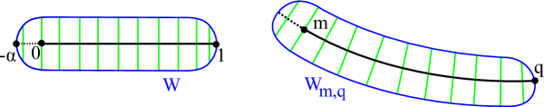
Construction of the domain $W_{m,q}$

6 Upper bound for harmonic measures

The main goal of this section is to obtain, in Corollary 6.20, the upper bound for the harmonic measures on $M$ needed for the proof of Proposition 4.8.

One of the major technical tools for estimating or constructing harmonic functions on Hadamard manifolds is the so-called Anderson-Schoen barriers. Given two opposite geodesic rays in a pinched Hadamard manifold, the corresponding Anderson-Schoen barrier is a positive superharmonic function that decreases exponentially along one of the geodesics rays, and is greater than 1 on a cone centered around the other geodesic ray [3].

Our first step is to obtain an analogous to the Anderson-Schoen barrier functions for the quotient manifold $M=\Gamma\backslash X$ in Proposition 6.18. This will rely on the work by Ancona [1], Anderson [2] and Anderson-Schoen [3].

In the whole section, $X$ will denote our pinched Hadamard manifold satisfying (1.2). The torsion-free convex cocompact subgroup $\Gamma$ of ${\rm Is\,}(X)$ will only come into the picture starting from Paragraph 6.4.

6.1 Harmonic measures at infinity on $X$

We first recall some fundamental, and by now classical, results concerning harmonic measures on Hadamard manifolds.

In the sequel $T,\alpha,c_{\circ},c_{r}\geq 1$ will be various constants such that $T,\alpha,c_{\circ}$ depend only on the pinched Hadamard manifold $X$, and $c_{r}$ also depends on the distance $r>0$.

Let us first recall the following Harnack-type inequality, due to Yau.

Lemma 6.1

[26] For a positive harmonic function $\eta:B(x,1)\subset X\to\mathopen{]}0,\infty\mathclose{[}$ defined on a ball with radius $1$, one has $|D_{x}(\log\eta)|\leq c_{1}$.

Another fundamental tool is the Green function $G:X\times X\to\mathopen{]}0,\infty]$. This Green function is continuous on $X\times X$, and is uniquely defined by the conditions

$$\Delta_{y}G(x,y) =-\delta_{x}$$

$$\lim_{y\to\infty}G(x,y) =0\,$$

for every $x\in X$. One can prove that $G$ is symmetric i.e. $G(x,y)=G(y,x)$ for $x,y$ in $X$. Moreover, the Green function satisfies the following estimates.

Proposition 6.2

1. If $d(x,y)\geq 1$, one has

$$c_{\circ}^{-1}\,d(x,y)-c_{\circ}\leq\log(1/G(x,y))\leq c_{\circ}\,d(x,y)+c_{\circ}\,.$$ (6.1)

2. Let $x,y,z\in X$ such that $d(x,y)\geq 1$ and $d(y,z)\geq 1$. One has

$$c_{\circ}^{-1}\,G(x,y)\,G(y,z)\leq G(x,z)\,.$$ (6.2)

If $d(x,z)\geq 1$ and $d(y,[x,z])\leq r$, one has

$$G(x,z)\leq c_{r}\,G(x,y)\,G(y,z)\,.$$ (6.3)

The first assertion is (2.4) in Anderson-Schoen [3]. The second assertion follows from (6.1), using Harnack inequality and the maximum principle, while the third one is Ancona’s inequality [1, Theorem 5].

Let us now turn to the bounded harmonic functions on $X$. Anderson proved in [2] that the Dirichlet problem at infinity on $X$ has a unique solution for any continuous boundary value. Hence there exists, for every point $x\in X$, a unique Borel measure $\omega_{x}$ on $\partial_{\infty}X$ such that, for any continuous function $u\in C^{0}(\partial_{\infty}X)$, the function

$$\eta_{u}:x\in X\to\int_{\partial_{\infty}X}u(\xi)\,d\omega_{x}(\xi)\in{\mathbb{R}}$$

is harmonic on $X$ and extends continuously to $\overline{X}$ with boundary value at infinity equal to $u$. The measure $\omega_{x}$ is the harmonic measure on $\partial_{\infty}X$ at the point $x$. The Harnack inequality of Lemma 6.1 ensures that two such harmonic measures $\omega_{x}$ and $\omega_{y}$ are absolutely continuous with respect to each other, and that their Radon-Nikodym derivatives $\frac{d\omega_{y}}{d\omega_{x}}$ are uniformly bounded when $d(x,y)\leq 1$. We will also need a control on these Radon-Nikodym derivatives for $d(x,y)\geq 1$, that will be given in Lemma 6.3.

In [3], Anderson-Schoen study the positive harmonic functions on $X$, and provide an identification of the Martin boundary of $X$ with the boundary at infinity $\partial_{\infty}X$. More precisely, they obtain the following results.

Fix a base point $o\in X$ and introduce the normalized Green function at the point $o\in X$ with pole at $z\in X$, which is defined by

$$k(o,x,z)=\frac{G(z,x)}{G(z,o)}\,.$$

Letting the point $z\in X$ converge to $\xi\in\partial_{\infty}X$, the limit

$$k(o,x,\xi)=\lim_{z\to\xi}k(o,x,z)\,$$

exists and $x\to k(o,x,\xi)$ is now a positive harmonic function on the whole $X$ that extends continuously to the zero function on $\partial_{\infty}X\smallsetminus\{\xi\}$, and such that $k(o,o,\xi)=1$.

In [3, Theorem 6.5] Anderson-Schoen prove that these positive harmonic functions are the minimal ones. Using the Choquet representation theorem, they provide the following Martin representation formula. For any positive harmonic function $\eta$ on $X$, there exists a unique finite positive Borel measure $\mu_{\eta}$ on $\partial_{\infty}X$ such that, for every $x\in X$,

$$\eta(x)=\int_{\partial_{\infty}X}k(o,x,\xi)\,d\mu_{\eta}(\xi)\,.$$

The minimal harmonic functions relate to the harmonic measures at infinity.

Lemma 6.3

1. Let $o,x\in X$. The following holds for $\omega_{o}$-a.e. $\xi\in\partial_{\infty}X$ :

$$k(o,x,\xi)=\frac{d\omega_{x}}{d\omega_{o}}(\xi)\,.$$ (6.4)

2. For $o,x\in X$ and $\xi\in\partial_{\infty}X$ with $d(o,x)\geq 1$, we have

$$k(o,x,\xi)\,G(o,x)\leq c_{\circ}\,.$$

If moreover $d(x,[o,\xi[)\leq r$, then we also have

$$c_{r}^{-1}\leq k(o,x,\xi)\,G(o,x)\,.$$

Proof  1. is proved in [3, §6].

2. follows readily from (6.2) and (6.3), with $z\in[o,\xi[$ and letting $z\to\xi$. $\Box$

Lemma 6.3 asserts that, if $d(o,x)\geq 1$ then, for every $\xi\in\partial_{\infty}X$ which is in the shadow of the ball $B(x,r)$ seen from $o$, all the densities $\frac{d\omega_{x}}{d\omega_{o}}(\xi)$ are close to $(G(o,x))^{-1}$ hence do not depend too much on $\xi$.

6.2 The action of ${\rm Is\,}(X)$ on $\partial_{\infty}X$

We now investigate, using Lemma 6.3, the action of ${\rm Is\,}(X)$ on the harmonic measures at inifinity.

Introduce the function defined, for any pair of points $x,y\in X$, by

$$d_{G}(x,y)=\log^{+}(1/G(x,y))$$

where $\log^{+}(t)=\sup(\log t,0)$ denotes the positive part of the logarithm. Proposition 6.2 tells us that, at large scale, the function $d_{G}$ behaves roughly like a distance that would be quasi-isometric to the Riemannian distance $d$. In particular, (6.2) ensures that there exists a constant $c_{\circ}$ such that the following weak triangle inequality holds for every $x,y,z\in X$:

$$d_{G}(x,z)\leq d_{G}(x,y)+d_{G}(y,z)+c_{\circ}\,.$$ (6.5)

Although $d_{G}$ is not exactly a distance on $X$, we will thus nevertheless agree to think of $d_{G}$ as of the Green distance. We would like to mention that Blachère-Haïssinski-Mathieu [7] already used such a Green distance in the similar context of random walks on hyperbolic groups.

From now on, we choose a base point $o\in X$. We associate to $d_{G}$ an analog to the Busemann functions by letting, for $\xi\in\partial_{\infty}X$ and $x\in X$ :

$$\beta_{\xi}(o,x)=-\log k(o,x,\xi)=\lim_{z\to\xi}d_{G}(x,z)-d_{G}(o,z)\,.$$

These Busemann functions relate to the harmonic measures at infinity, since (6.4) reads as

$$\frac{d\omega_{x}}{d\omega_{o}}(\xi)=e^{-\beta_{\xi}(o,x)}\,.$$ (6.6)

Define the length of $g\in{\rm Is\,}(X)$ as $|g|_{o}=d_{G}(o,go)$. We want to compare $\beta_{\xi}(o,g^{-1}o)$ with $|g|_{o}$.

Notation 6.4

When $g\in{\rm Is\,}(X)$ does not fix the point $o$, we introduce the endpoints $\xi_{{}_{+}}\!(g),\xi_{{}_{-}}\!(g)\in\partial_{\infty}X$ of the geodesic rays with origin $o$ that contain respectively the points $go$ and $g^{-1}o$.

Lemma 6.5

(1) For $g\in{\rm Is\,}(X)$ and $\xi\in\partial_{\infty}X$, one has $|g|_{o}=|g^{-1}|_{o}$ and

$$|\beta_{\xi}(o,g^{-1}o))|\leq|g|_{o}+c_{\circ}\,.$$

(2) For every $\varepsilon>0$ there exists a constant $a_{\varepsilon}\geq 1$ such that, when $g\in{\rm Is\,}(X)$ and $\xi\in\partial_{\infty}X$ satisfy $\angle_{o}(\xi,\xi_{{}_{-}}\!(g))\geq\varepsilon$, then

$$|g|_{o}\leq\beta_{\xi}(o,g^{-1}o)+a_{\varepsilon}\,.$$

Proof  (1) We observe that, since the Green function $G$ is symmetric and invariant under isometries, we have $d_{G}(y,x)=d_{G}(x,y)=d_{G}(gx,gy)$ for every $g\in{\rm Is\,}(X)$ and $x,y\in X$. The equality $|g|_{o}=|g^{-1}|_{o}$ follows.

Using the weak triangle inequality (6.5) for $d_{G}$ yields

$$\beta_{\xi}(o,g^{-1}o)=\lim_{z\to\xi}d_{G}(g^{-1}o,z)-d_{G}(o,z)\leq d_{G}(g^{-1}o,o)+c_{\circ}=|g|_{o}+c_{\circ}\,.$$

The lower bound follows by observing that the invariance of $d_{G}$ under isometries ensures that

$$\beta_{\xi}(o,g^{-1}o)=\beta_{g\xi}(go,o)=-\beta_{g\xi}(o,go)\geq-|g|_{o}-c_{\circ}\,.$$

(2) We may suppose that $|g|_{o}>0$ so that $|g|_{o}=-\log G(o,g^{-1}o)$. Since $K_{X}\leq-a^{2}$, the condition $\angle_{o}(\xi,\xi_{{}_{-}}\!(g))\geq\varepsilon$ ensures that the distance of the point $o$ to the geodesic ray $\mathopen{[}g^{-1}(o),\xi\mathclose{[}$ is bounded above by a constant $r_{\varepsilon}$ that depends only on $\varepsilon$. Lemma 6.3 (2) yields $|g|_{o}\leq\beta_{\xi}(o,g^{-1}o)+\log c_{r_{\varepsilon}}$. $\Box$

The following corollary provides useful estimates for action of isometries on the harmonic measures on $\partial_{\infty}X$.

Corollary 6.6

For $A\subset\partial_{\infty}X$ a measurable set and $g\in{\rm Is\,}(X)$, one has

$$e^{-c_{\circ}}e^{-|g|_{o}}\omega_{o}(A)\leq\omega_{o}(gA)\leq e^{c_{\circ}}e^{|g|_{o}}\omega_{o}(A)\,.$$

If we assume that $\angle_{o}(\xi,\xi_{{}_{-}}\!(g))\geq\varepsilon$ for every $\xi\in A$, one has

$$\omega_{o}(gA)\leq e^{a_{\varepsilon}}e^{-|g|_{o}}\omega_{o}(A)\,$$

where $a_{\varepsilon}$ is the constant in Lemma 6.5.

Proof  Immediate consequence of Lemma 6.5 and Equality (6.6). $\Box$

6.3 Harmonic measures of cones in $X$

We now recall estimates for the harmonic measures at infinity, that are due to Anderson-Schoen.

Definition 6.7

Let $o\in X$, $\xi\in\partial_{\infty}X$ and $\theta\in[0,\pi]$. The closed cone ${\cal C}_{o\xi}^{\theta}\subset X$ with vertex $o$, axis $[o,\xi\mathopen{[}$ and angle $\theta$ is the union of all the geodesic rays $[o,\zeta\mathopen{[}$ whose angle with $[o,\xi\mathopen{[}$ is at most $\theta$. The trace of the cone ${\cal C}_{o\xi}^{\theta}$ on the sphere at infinity $\partial_{\infty}X$ will be denoted by ${\cal S}_{o\xi}^{\theta}$.

By analogy with the case where $X$ has constant curvature, we will take the liberty of calling a cone ${\cal D}_{o\xi}:={\cal C}_{o\xi}^{\pi/2}\subset X$ with angle $\theta=\pi/2$ a closed half-space, with vertex $o$, and its boundary ${\cal H}_{o\xi}$ a hyperplane, also with vertex $o$. We will denote by ${\cal S}_{o\xi}$ the trace of the half-space ${\cal D}_{o\xi}$ on the boundary at infinity, and we will call it a half-sphere at infinity seen from the point $o$.

Although half-spaces in the pinched Hadamard manifold $X$ may not be convex, the following lemma tells us that they are not far from being so.

Lemma 6.8

[8, Prop.2.5.4] There exists a constant $\lambda$, that depends only on the pinching constants of $X$, such that the convex hull of a half-space ${\cal D}\subset X$ lies within its $\lambda$-neighbourhood : ${\rm Hull}\,({\cal D})\subset{\cal V}_{\lambda}({\cal D})$.

Proof  This statement follows from Proposition 2.15, due to Bowditch. Observe indeed that ${\cal D}$ is included in the join of its half-sphere ${\cal S}$ at infinity, and that this join lies in the $\delta_{X}$-neighbourhood of ${\cal D}$. $\Box$

The following uniform bounds for harmonic measures of cones in pinched Hadamard manifolds are due to Anderson-Schoen.

Lemma 6.9

There exists a constant $c_{\circ}\geq 1$ such that one has, for any point $o\in X$ and any $\xi\in\partial_{\infty}X$,

$$\omega_{o}({\cal S}_{o\xi}^{\pi/4})\geq 1/c_{\circ}\,.$$

A more precise statement is given by Kifer-Ledrappier in [16, Theorem 4.1].

Notation 6.10

We now fix a base point $o\in X$. When $\xi\in\partial_{\infty}X$, we denote by $t\in{\mathbb{R}}\to x_{\xi}^{t}\in X$ the unit speed geodesic with origin $o$ that converges to $\xi\in\partial_{\infty}X$ in the future. We will let ${\cal D}_{\xi}^{t}$ stand for the half-space ${\cal D}_{x^{t}_{\xi}\xi}$ with vertex $x^{t}_{\xi}$ and axis $[x^{t}_{\xi},\xi\mathopen{[}$, and will denote accordingly by ${\cal H}_{\xi}^{t}$ and ${\cal S}_{\xi}^{t}$ the corresponding hyperplane and half-sphere at infinity.

Proposition 6.11

There exist a distance $T>0$ and two constants $\alpha>0$ and $c_{\circ}\geq 1$ such that the following holds for every $\xi\in\partial_{\infty}X$ :

$$\omega_{x^{-t}_{\xi}}({\cal S}_{o\xi}) \leq c_{\circ}\,e^{-\alpha t} t\geq 0$$ for every

$$\omega_{y}({\cal S}_{o\xi}) \geq 1/c_{\circ} y\in{\cal D}_{\xi}^{T}$$ for every .

Proof  The first assertion is [3, Corollary 4.2].

Thanks to the upper bound on the curvature $K_{X}$ of $X$, there exists a distance $T>0$ that depends only on $X$ such that the half-space ${\cal D}_{\xi}^{T}$ is seen from the point $o$ under an angle at most $\pi/4$, namely such that ${\cal D}_{\xi}^{T}\subset{\cal C}_{o\xi}^{\pi/4}$.

If now $y\in{\cal D}_{\xi}^{T}$ and $\zeta_{y}\in\partial_{\infty}X$ denotes the endpoint of the geodesic ray such that $y\in[o,\zeta_{y}\mathclose{[}$, it follows that ${\cal C}_{y\zeta_{y}}^{\pi/4}\subset{\cal D}_{o\xi}$. Lemma 6.9 yields $\omega_{y}({\cal S}_{o\xi})\geq\omega_{y}({\cal S}_{y\zeta_{y}}^{\pi/4})\geq 1/c_{\circ}$. $\Box$

6.4 Geometry in embedded half-spaces in $M$

In this paragraph, we introduce embedded half-spaces in the quotient $M=\Gamma\backslash X$ (Proposition 6.16), that will be needed in the sequel of this paper.

Recall that we fixed a base point $o\in X$. We keep Notation 6.10.

Notation 6.12

We now introduce the projection $m_{0}\in M=\Gamma\backslash X$ of our base point $o\in X$. When $\xi\in\partial_{\infty}X$, we will denote by $t\in{\mathbb{R}}\to m^{t}_{\xi}\in M$ the (perhaps non minimizing) geodesic obtained by projection of the geodesic $t\in{\mathbb{R}}\to x_{\xi}^{t}\in X$.

Definition 6.13

A closed embedded half-space with vertex $m_{\xi}^{t}$ is the projection in $M$ of a closed half-space ${\cal D}_{\xi}^{t}\subset X$ that embeds in $M$, namely that satisfies $\overline{\cal D}_{\xi}^{t}\cap\gamma\overline{\cal D}_{\xi}^{t}=\emptyset$ for every non trivial element $\gamma\in\Gamma$, where $\overline{\cal D}_{\xi}^{t}\subset\overline{X}$ denotes the closure of ${\cal D}_{\xi}^{t}$ in the compactification of $X$.

We first remark that there exist many embedded half-spaces in $M$. Choose a relatively compact subset $\Omega_{0}\subset\Omega_{\Gamma}$ of the domain of discontinuity.

Lemma 6.14

There exists $t_{0}>0$ such that, for every $\xi\in\Omega_{0}$ and every $t\geq t_{0}$, the half-space ${\cal D}_{\xi}^{t}\subset X$ embeds in $M$.

Proof  We proceed by contradiction, and assume that there exist sequences $t_{n}\to+\infty$, $\xi_{n}\in\Omega_{0}$, $z_{n}\in\overline{\cal D}_{\xi_{n}}^{t_{n}}$ and $\gamma_{n}\in\Gamma^{*}$ such that $\gamma_{n}z_{n}\in\overline{\cal D}_{\xi_{n}}^{t_{n}}$ for every $n\in{\mathbb{N}}$. By compactness of $\Omega_{0}$, we may assume that the sequence $(\xi_{n})$ converges to some $\xi_{\infty}\in\Omega_{0}$. Since $t_{n}\to\infty$ and $\xi_{n}\to\xi_{\infty}$, both sequences $(z_{n})$ and $(\gamma_{n}z_{n})$ converge to $\xi_{\infty}$ in $\overline{X}$. Since the action of $\Gamma$ on $X\cup\Omega_{\Gamma}$ is properly discontinuous, and $\Gamma$ is torsion-free, it follows that $\gamma_{n}$ is trivial for $n$ large, a contradiction. $\Box$

Notation 6.15

For $\xi\in\Omega_{0}$ and $t\geq t_{0}$, we will denote by the Roman letters $D_{\xi}^{t}\subset M$ the closed embedded half-space with vertex $m_{\xi}^{t}$ and by $H_{\xi}^{t}$ its boundary in $M$, respectively obtained as the projections of ${\cal D}_{\xi}^{t}$ and ${\cal H}_{\xi}^{t}$.

Our goal in the remaining of this section is to prove that an embedded half-space in the quotient $M=\Gamma\backslash X$ is not far from being geodesically convex :

Proposition 6.16

There exists $\tau_{0}\geq 1$ such that, for every $\xi\in\Omega_{0}$ and $t\geq t_{0}$, and for every pair of points $p_{1},p_{2}\in D_{\xi}^{t+\tau_{0}}$, there exists only one minimizing geodesic segment $[p_{1},p_{2}]\subset M$, and it lies in $D_{\xi}^{t}$.

Proposition 6.16 relies on an analogous property for the half-space ${\cal D}_{\xi}^{t+t_{0}}$ in the pinched Hadamard manifold $X$ that we proved in Lemma 6.8. We first state an elementary property of obtuses triangles in $X$.

Lemma 6.17

There exists a constant $\hat{\delta}_{0}$ that depends only on $X$ such that if $[y,x,z]\subset X$ is a triangle with an angle at least $\pi/2$ at the vertex $x$, then $d(y,z)\geq d(x,y)+d(y,z)-\hat{\delta}_{0}$.

Proof  Same as for Lemma 2.8. $\Box$

Proof of Proposition 6.16 Let $\tau_{0}>0$ and $p_{1},p_{2}\in D_{\xi}^{t+\tau_{0}}$. Consider a minimizing geodesic segment $[p_{1},p_{2}]\subset M$. Lift the points $p_{1},p_{2}\in D_{\xi}^{t+\tau_{0}}$ as $y_{1},y_{2}\in{\cal D}_{\xi}^{t+\tau_{0}}$. Then, there exists $\gamma\in\Gamma$ such that $[p_{1},p_{2}]$ lifts as a geodesic segment $[y_{1},\gamma y_{2}]\subset X$.

Assume first that $\gamma=e$. If we choose $\tau_{0}\geq\lambda_{X}$, the $\lambda_{X}$-neighbourhood of the half-space ${\cal D}_{\xi}^{t+\tau_{0}}$ lies in ${\cal D}_{\xi}^{t}$. Hence, it follows from Lemma 6.8 that $[y_{1},y_{2}]\subset{\cal D}_{\xi}^{t}$ so that $[p_{1},p_{2}]\subset D_{\xi}^{t}$.

Proceed now by contradiction and assume that $\gamma\in\Gamma^{*}$ is non trivial. Observe that, since the boundary of ${\cal D}_{\xi}^{t}$ is a union of geodesic rays emanating from the point $x_{\xi}^{t}$, the geodesic segment $\mathopen{]}x_{\xi}^{t},\gamma x_{\xi}^{t}\mathclose{[}$ stays out of both half-spaces ${\cal D}_{\xi}^{t}$ and $\gamma{\cal D}_{\xi}^{t}$.

Let $\varepsilon=\inf\{d(y,\gamma y)\;|\,y\in X,\;\gamma\in\Gamma^{*}\}>0$, and $\alpha_{\varepsilon}$ be the corresponding angle in Lemma 2.8. As in the proof of Proposition 6.11, choose $\tau_{0}$ large enough so that any half-space ${\cal D}_{\xi}^{t+\tau_{0}}$ is seen from the point $x_{\xi}^{t}$ under an angle less than $\alpha_{\varepsilon}$. We may then apply Lemma 2.8 to the quadrilateral $[y_{1},x_{\xi}^{t},\gamma x_{\xi}^{t},\gamma y_{2}]\subset X$ to obtain

$$d(y_{1},\gamma y_{2}) \geq d(y_{1},x_{\xi}^{t})+d(x_{\xi}^{t},\gamma x_{\xi}^{t})+d(\gamma x_{\xi}^{t},\gamma y_{2})-2\tilde{\delta}_{\varepsilon}$$

$$\geq d(y_{1},x_{\xi}^{t})+d(y_{2},x_{\xi}^{t})-2\tilde{\delta}_{\varepsilon}\,.$$

Applying Lemma 6.17 to each triangle $[y_{i},x_{\xi}^{t+\tau_{0}},x_{\xi}^{t}]$ ($i=1,2$) yields

$$d(y_{i},x_{\xi}^{t})\geq d(y_{i},x_{\xi}^{t+\tau_{0}})+\tau_{0}-\hat{\delta}_{0}\,.$$

This is a contradiction if $\tau_{0}>(\hat{\delta}_{0}+\hat{\delta}_{\varepsilon})$, since the triangle inequality yields

$$d(y_{1},\gamma y_{2})\geq d(y_{1},y_{2})+2\tau_{0}-2(\hat{\delta}_{0}+\hat{\delta}_{\varepsilon})\,. \Box$$

6.5 Harmonic measures and embedded half-spaces in $M$

To construct an analogous to the Anderson-Schoen barrier functions for the quotient manifold $M=\Gamma\backslash X$, we work in the Hadamard manifold $X$.

Recall that we fixed a base point $o\in X$ and that $\Omega_{0}\subset\Omega_{\Gamma}$ is relatively compact. We keep the notation of Proposition 6.11 and Lemma 6.14.

Proposition 6.18

There exists $C_{0}\geq 1$ such that, for every $\xi\in\Omega_{0}$, the harmonic measure at infinity of the saturation of ${\cal S}_{\xi}^{t}$ under $\Gamma$ satisfies

$$\omega_{o}\bigl{(}\bigcup_{\gamma\in\Gamma}\gamma\,{\cal S}_{\xi}^{t}\bigr{)} \leq C_{0}\,e^{-\alpha t} t\geq t_{0}$$ for every

$$\omega_{y}\bigl{(}\bigcup_{\gamma\in\Gamma}\gamma\,{\cal S}_{\xi}^{t}\bigr{)} \geq 1/C_{0} y\in{\cal D}_{\xi}^{t+T}$$ for every .

We will need the following fact relative to the domain of discontinuity of $\Gamma$.

Lemma 6.19

Let $L\subset\Omega_{\Gamma}$ be any compact subset of the domain of discontinuity. Then, there is only a finite number of elements $\gamma\in\Gamma^{*}$ with $\gamma o\neq o$ and $\xi_{{}_{-}}\!(\gamma)\in L$.

Proof  Let $(\gamma_{n})$ be a sequence of pairwise distinct elements of $\Gamma$ such that $\xi_{{}_{-}}\!(\gamma_{n})\to\zeta\in\partial_{\infty}X$. Since $\Gamma$ is discrete, $d(\gamma_{n}^{-1}o,o)\to\infty$ so that $\gamma_{n}^{-1}o\to\zeta$ hence $\zeta\in\Lambda_{\Gamma}$. The result follows readily. $\Box$

Proof of Proposition 6.18 The lower bound is an immediate consequence of Proposition 6.11.

Let now $\varepsilon>0$ small enough so that $\angle_{o}(\xi,\Lambda_{\Gamma})\geq 2\varepsilon$ for every $\xi\in\Omega_{0}$. Lemma 6.19 ensures that the set $\Gamma_{\varepsilon}=\{\gamma\in\Gamma^{*}\,|\;\angle_{o}(\xi_{{}_{-}}\!(\gamma),\Lambda_{\Gamma})\geq\varepsilon\}$ is finite.

Assuming that $t\geq t_{0}$, we now seek an upper bound for $\omega_{o}(\bigcup_{\gamma\in\Gamma}\gamma\,{\cal S}_{\xi}^{t})$. We first observe that Corollary 6.6 and Lemma 6.14 ensure that

$$e^{-c_{\circ}}\omega_{o}({\cal S}_{\xi}^{t})\;\bigl{(}\sum_{\gamma\in\Gamma}e^{-|\gamma|_{o}}\bigr{)}\leq\sum_{\gamma\in\Gamma}\omega_{o}(\gamma\,{\cal S}_{\xi}^{t})=\omega_{o}(\bigcup_{\gamma\in\Gamma}\gamma\,{\cal S}_{\xi}^{t})\,,$$

so that the series $\sum_{\gamma\in\Gamma}e^{-|\gamma|_{o}}$ converges. When $\gamma\in\Gamma\smallsetminus\Gamma_{\varepsilon}$ is non trivial, one has $\angle_{o}(\xi,\xi_{{}_{-}}\!(\gamma))\geq\varepsilon$ for every $\xi\in\Omega_{0}$. Hence Corollary 6.6 again yields

$$\sum_{\gamma\in\Gamma}\omega_{o}(\gamma\,{\cal S}_{\xi}^{t}) \leq\Bigl{(}e^{c_{\circ}}\,\sum_{\Gamma_{\varepsilon}}e^{|\gamma|_{o}}+e^{a_{\varepsilon}}\,\sum_{\Gamma\smallsetminus\Gamma_{\varepsilon}}e^{-|\gamma|_{o}}\Bigr{)}\;\omega_{o}({\cal S}_{\xi}^{t})\,,$$

and the claim now follows from Proposition 6.11. $\Box$

Recall that $V$ is the compact convex subset of $M$ that we introduced in Proposition 4.2. From now on, we will assume that the base point $o\in X$ is so chosen that its projection $m_{0}\in M$ belongs to $V$.

Corollary 6.20

Upper bound for harmonic measures on $M$

There exists a constant $C_{1}$ such that the following holds. For every compact domain with smooth boundary $W$ whose interior contains $V$, every $\xi\in\Omega_{0}$, every $t\geq 0$ and every point $m\in V$ :

$$\sigma_{m,W}(\partial W\cap D_{\xi}^{t})\leq C_{1}e^{-\alpha t}\,.$$ (6.7)

Proof  It suffices to prove the assertion when $t$ is large. Recall that $T$ has been defined in Proposition 6.11. For $\xi\in\Omega_{0}$ and $t\geq t_{0}+T$, introduce the positive harmonic function defined by

$$\tilde{\eta}_{\xi}^{t}:y\in X\to\omega_{y}\bigl{(}\bigcup_{\gamma\in\Gamma}\gamma\,{\cal S}_{\xi}^{t-T}\bigr{)}\in[0,1]\,.$$

The function $\tilde{\eta}_{\xi}^{t}$ is $\Gamma$-invariant and thus goes to the quotient to a harmonic function $\eta_{\xi}^{t}:M\to[0,1]$. Proposition 6.18 (that we apply to $t-T\geq t_{0}$) ensures that $\eta_{\xi}^{t}$ satisfies

$$\eta_{\xi}^{t}(p) \geq 1/C_{0} p\in D_{\xi}^{t}$$ for every

$$\eta_{\xi}^{t}(m_{0}) \leq C_{0}e^{\alpha T}\,e^{-\alpha t}\,.$$

Applying the Harnack inequality (Lemma 6.1) to $\tilde{\eta}_{\xi}^{t}$ yields

$$\eta_{\xi}^{t}(m)\leq e^{c_{1}d_{V}}C_{0}e^{\alpha T}\,e^{-\alpha t}\quad\hbox{for every $m\in V$,}$$ (6.8)

where $d_{V}$ denotes the diameter of the compact convex set $V$.

The function $C_{0}\,\eta_{\xi}^{t}$ is everywhere positive, and is greater or equal to $1$ on $\partial W\cap D_{\xi}^{t}$. Thus, the maximum principle ensures that

$$C_{0}\,\eta_{\xi}^{t}(p)\geq\sigma_{p,W}(\partial W\cap D_{\xi}^{t})$$

holds for every $p\in W$, and the claim now follows from (6.8). $\Box$

Note that the constants $t_{0}$, $\tau_{0}$, $C_{0}$ and $C_{1}$ that we introduced in the previous paragraphs depend only on the group $\Gamma$, on the base point $o$, on $\Omega_{0}$ and on the compact subset $V\subset M$.

6.6 Gromov products and embedded half-spaces

We end this chapter with Proposition 6.21, that relates half-spaces corresponding to the same point at infinity with level sets of Gromov products.

Recall that we choose a base point $o\in X$ whose projection $m_{0}\in M$ lies in the compact subset $V\subset M$ and that $t_{0}$ and $\tau_{0}\geq 1$ were defined in Lemma 6.14 and Proposition 6.16.

Proposition 6.21

There exists a constant $g$ such that, for every $\xi\in\Omega_{0}$, every $t\geq t_{0}+\tau_{0}$, every point $p\in D_{\xi}^{t+\tau_{0}}$ and every point $m\in V$ :

$$\{q\in M\ |\ (p,q)_{m}\geq t+g\}\subset D_{\xi}^{t}\,.$$

Proof  Let $p\in D_{\xi}^{t+\tau_{0}}$ and $q\notin D_{\xi}^{t}$. Consider a minimizing geodesic segment $[p,q]\subset M$ and introduce two points $p^{\prime}$ and $q^{\prime}$ where $[p,q]$ intersects the hyperplanes $H_{\xi}^{t+\tau_{0}}$ and $H_{\xi}^{t}$.

Since $t\geq t_{0}+\tau_{0}$, it follows from Proposition 6.16 that any, hence the only, minimizing quadrilateral $[p^{\prime},m_{\xi}^{t+\tau_{0}},m_{\xi}^{t},q^{\prime}]$ lies in the embedded half-plane $D_{\xi}^{t_{0}}$ and is thus isometric to a quadrilateral in $X$.

This quadrilateral $[p^{\prime},m_{\xi}^{t+\tau_{0}},m_{\xi}^{t},q^{\prime}]$ is right-angled at both vertices $m_{\xi}^{t}$ and $m_{\xi}^{t+\tau_{0}}$, and $d(m_{\xi}^{t},m_{\xi}^{t+\tau_{0}})=\tau_{0}\geq 1$. Hence Lemma 2.8 applies to prove that the point $m_{\xi}^{t}$ is within distance $\tilde{\delta}_{1}$ of the edge $[p^{\prime},q^{\prime}]$. Since $[p^{\prime},q^{\prime}]\subset[p,q]$ and $d(m,m_{\xi}^{t})\leq t+d_{V}$, it follows from Lemma 2.2 that

$$(p,q)_{m}\leq d(m,[p,q])\leq d(m,[p^{\prime},q^{\prime}])\leq t+(d_{V}+\tilde{\delta}_{1})\,.$$

The claim follows for $g>d_{V}+\tilde{\delta}_{1}$. $\Box$

7 Interior estimates

In this final section, we wrap up the proof of Proposition 4.8, that gives a uniform bound for the distances $d(f,h_{R})$.

We split the proof into two parts. In the first part, where we assume that the point $m\in V_{R}$ where the distance $d(f,h_{R})$ is reached lies far away from the convex core, the proof reduces to the proof of the main theorem of [6].

In the second part, where we assume that the point $m$ lies in a fixed neighbourhood of the convex core, we must deal with the topology of the quotient $M=\Gamma\backslash X$.

7.1 Harmonic quasi-isometric maps $H:X\to Y$

In [6], we proved that a quasi-isometric map $F:X\to Y$ between two pinched Hadamard manifolds $X$ and $Y$ is within bounded distance from a unique harmonic map. As in the present paper, this harmonic map was obtained as the limit of a family of solutions of Dirichlet problems on bounded domains with boundary value $F$, where a uniform bound for the distances between $F$ and the solutions of these Dirichlet problems ensured the convergence of the family.

In the following technical statement, which is local in nature, we gather some information obtained in [6] that was used to obtain this uniform bound. The first part of our proof of Proposition 4.8 will derive easily from this statement, see Proposition 7.3.

Fact 7.1

Let $c\geq 1$. There exist $\ell_{0}>1$ and $\rho_{0}>0$ with the following property.

Let $F,H:B(x,\ell_{0})\to Y$ be two smooth maps defined on a ball $B(x,\ell_{0})\subset X$ with radius $\ell_{0}$, and such that the distance

$$\rho:=\sup_{z\in B(x,\ell_{0})}d(F(z),H(z))$$

is reached at the center $x$ of the ball, namely $\rho=d(F(x),H(x))$. Assume that $H$ is harmonic and that the map $F$ satisfies

$$c^{-1}d(z,z^{\prime})-c\leq d(F(z),F(z^{\prime}))\leq c\,d(z,z^{\prime}) z,z^{\prime}\in B(x,\ell_{0})$$ for any , (7.1)

Then

$$\rho\leq\rho_{0}\,.$$

Proof  This fact is proven in [6, Section 4]. Alternatively, one may follow paragraphs 7.3 through 7.5 below, replacing the domain $V_{\ell}$ with the ball $B(m,\ell_{0})$ and using the uniform estimates (5.2) for the harmonic measures of balls in the Hadamard manifold $X$ instead of the new estimates (5.3) and (6.7). $\Box$

7.2 Part one : estimate far away from the core

In this paragraph, we introduce a finite family of embedded half-spaces in $M$, whose union is a neighbourhood of infinity, and that will be used throughout the proof of Proposition 4.8. Then, we prove Proposition 4.8 in case the distance $d(f,h_{R})$ is reached far away from the convex core.

Recall that, after smoothing, the map $f:M\to Y$ is assumed to be $c$-Lipschitz (4.1) and that each point $\xi\in\partial_{\infty}M$ admits a neighbourhood to which $f$ restricts as a quasi-isometric map.

From now on, $\Omega_{0}\subset\Omega_{\Gamma}$ is a fixed compact neighbourhood of a fundamental domain for the action of $\Gamma$ on $\Omega_{\Gamma}$.

Lemma 7.2

(1) There exists a finite number of embedded half-spaces $D_{\zeta_{i}}^{t_{i}}$ ($1\leq i\leq N$) with $\zeta_{i}\in\Omega_{0}$ and $t_{i}\geq t_{0}$ such that, taking perhaps a larger constant $c$ in (4.1) :

• each restriction $f:D_{\zeta_{i}}^{t_{i}}\to Y$ is a quasi-isometric map with constant $c$

• $\cup_{i=1}^{N}D_{\zeta_{i}}^{t_{i}+\tau_{0}}$ is a neighbourhood of infinity in $M$.

(2) We may also assume that $V$ has been choosen large enough so that

$$\bullet\;\partial V\subset\cup_{i=1}^{N}D_{\zeta_{i}}^{t_{i}+\tau_{0}}$$ (7.2)

$$\bullet\;\hbox{for $m\notin V$, one has ${\rm inj}(m)\geq\ell_{0}$}$$ (7.3)

$$\bullet\;\hbox{for $m\notin V$, the restriction of $f$ to $B(m,\ell_{0})$ is $c$ quasi-isometric.}$$ (7.4)

Proof  (1) We proved in Lemma 6.14 that, for every $\xi\in\Omega_{0}$ and any $t\geq t_{0}$, the half-space $D_{\xi}^{t}$ embeds in $M$. Hence, the claim follows from the hypothesis on $f$, since the boundary at infinity $\partial_{\infty}M$ is compact.

(2) The injectivity radius ${\rm inj}:M\to[0,\infty[$ is a proper function, and the complement in $M$ of

$$\cup_{i=1}^{N}\{m\in M\;|\;B(m,\ell_{0})\subset D_{\zeta_{i}}^{t_{i}}\}$$

is bounded. Hence, it suffices to replace the convex set $V$ of Proposition 4.2 by its $R_{0}$-neighbourhood for some large $R_{0}$ to ensure these conditions. $\Box$

We want a uniform upper bound for the distance $d(f,h_{R})$ when $R$ is large. We may thus assume that

$$R\geq\ell_{0}+1\,.$$ (7.5)

In the next proposition, we obtain such a bound in case the distance $d(f,h_{R})$ is reached at some point $m$ which is far away from the convex core, that is if $m\notin V$. The case where $m\in V$ will be carried out in the next paragraphs.

Proposition 7.3

Suppose that the distance $d(f,h_{R})=d(f(m),h_{R}(m))$ is reached at some point $m\in V_{R}\smallsetminus V$. Then

$$d(f,h_{R})\leq\rho_{0}+B\ell_{0}\,,$$

where $B$ is the constant in Proposition 4.11, and $\rho_{0}$ is defined in Fact 7.1.

Proof  Assume first that $d(m,\partial V_{R})\leq\ell_{0}$. It follows from Proposition 4.11 that

$$d(f,h_{R})=d(f(m),h_{R}(m))\leq B\,d(m,\partial V_{R})\leq B\ell_{0}\,.$$

Assume now that $d(m,\partial V_{R})>\ell_{0}$, so that the ball $B(m,\ell_{0})$ lies in $V_{R}$. Since $m\notin V$, Condition (7.3) ensures that this ball $B(m,\ell_{0})$ is isometric to a ball with radius $\ell_{0}$ in the Hadamard manifold $X$. Fact 7.1 applies to the restrictions $F=f_{|B(m,\ell_{0})}$ and $H=(h_{R})_{|B(m,\ell_{0})}$, so that $\rho\leq\rho_{0}$. The result follows. $\Box$

7.3 Part two : estimate close to the core, an overview

To complete the proof of Proposition 4.8, we assume from now on that the distance $\rho=d(f,h_{R})$ is reached at some point $m$ that belongs to the fixed compact set $V$. We pick a large $\ell$ (namely $\ell$ will have to satisfy Conditions (7.6), (7.11) and (7.13)), and we will mainly work on the compact convex set with smooth boundary $V_{\ell}$ which is the $\ell$-neighbourhood of $V$. Note that $V_{\ell}$ does not depend on $R$.

We will assume that

$$\ell\geq d_{V}+1\,,$$ (7.6)

where $d_{V}$ denotes the diameter of the domain $V$. Since we want an upper bound for the distance $\rho=d(f,h_{R})$ when $R$ is large, we may also assume from now on that

$$\rho \geq c$$ (7.7)

$$R \geq\ell+2\,.$$ (7.8)

For any point $p$ in the $1$-neighbourhood of $V_{\ell}$, namely for $p\in V_{\ell+1}$, Condition (7.8) ensures that $B(p,1)\subset V_{R}$, so that Corollary 4.10 yields

$$\|D_{p}h_{R}\|\leq\kappa\rho\,.$$ (7.9)

We introduce $y=f(m)\in Y$, which is the image under $f$ of the point $m\in V$ where the distance $d(f,h_{R})$ is reached. For any point $p\in\partial V_{\ell}$, we shall study the three following Gromov products relative to this point $y$ :

$$g_{0}(p)=(f(p),h_{R}(m))_{y},\ g_{1}(p)=(f(p),h_{R}(p))_{y},\ g_{2}(p)=(h_{R}(p),h_{R}(m))_{y}\,.$$

If $\rho$ is large, we shall prove that on a suitable subset $U_{\ell,R}$ of the boundary $\partial V_{\ell}$, both $g_{1}$ and $g_{2}$ are large (Lemma 7.8 and Corollary 7.10) while the measure of $U_{\ell,R}$ is large enough (Lemma 7.5) to ensure that $g_{0}$ cannot be that large on the whole $U_{\ell,R}$ (Lemma 7.6). This will yield a contradiction thanks to Inequality (2.1) satisfied by Gromov products.

The arguments we develop here are similar to those of [6, Section 4], and that led to Fact 7.1. In the setting of our previous paper [6], they relied on the uniform upper and lower bounds for harmonic measures of balls in the Hadamard manifold relative to their center. In our new context, they rely on the uniform upper and lower bounds for harmonic measures obtained in Proposition 5.2 and Corollary 6.20.

7.4 The subset $U_{\ell,R}\subset\partial V_{\ell}$

We introduce the domain $U_{\ell,R}\subset\partial V_{\ell}$ that will play a central role in the proof of Proposition 4.8.

Definition 7.4

Let $U_{\ell,R}$ be the set of those points $p\in\partial V_{\ell}$ where the distance $d(y,h_{R}(p))$ is close to $\rho=d(y,h_{R}(m))$, namely

$$U_{\ell,R}=\{p\in\partial V_{\ell}\,|\;d(y,h_{R}(p))\geq\rho-\frac{\ell}{2c}\}\,.$$

In the next lemma, we give a lower bound for the “size” of the domain $U_{\ell,R}\subset\partial V_{\ell}$, which is uniform with respect to $R$ and to the choice of $\ell$.

Lemma 7.5

The harmonic measure $\sigma_{m,V_{\ell}}$ of the set $U_{\ell,R}\subset\partial V_{\ell}$ relative to the point $m\in V$ satisfies

$$\sigma_{m,V_{\ell}}(U_{\ell,R})\geq\,\frac{1}{5\,c^{2}}.$$

Proof  We first observe that, for any point $q\in V_{\ell}$, one has

$$d(y,h_{R}(q))\leq\rho+2c\,\ell\,.$$ (7.10)

Indeed, since by (4.1) the function $f$ is $c$-Lipschitz, the triangle inequality yields

$$d(f(m),h_{R}(q))\leq d(f(m),f(q))+d(f(q),h_{R}(q))\leq c\,(d_{V}+\ell)+\rho$$

where as usual $d_{V}$ denotes the diameter of $V$. Thus (7.10) follows, since we assumed in (7.6) that $\ell\geq d_{V}$.

Now, Lemma 3.5 asserts that the function $u:q\to d(y,h_{R}(q))-\rho$ is subharmonic on $V_{R}$. Moreover (7.10) ensures that $u$ is bounded above by $2c\,\ell$ on $V_{\ell}$. Since $u(m)=0$, this yields

$$0\leq\int_{\partial V_{\ell}}u(p)\,d\sigma_{m,V_{\ell}}(p)\leq\sigma_{m,V_{\ell}}(U_{\ell,R})\,(2c\,\ell)-(1-\sigma_{m,V_{\ell}}(U_{\ell,R}))\,\frac{\ell}{2c}\,,$$

thus $1\leq\sigma_{m,V_{\ell}}(U_{\ell,R})\,(1+4c^{2})$ hence the claim, since we assumed $c\geq 1$. $\Box$

7.5 Upper bound for the Gromov product $g_{0}(p)$ on $U_{\ell,R}$

In this paragraph we prove that, if $\ell$ is large enough, the Gromov products $g_{0}(p)=(f(p),h_{R}(m))_{y}$ cannot be uniformly large on the whole $U_{\ell,R}$.

We first prove that the image $f(U_{\ell,R})\subset Y$, seen from the point $y=f(m)$, is relatively spread out.

Lemma 7.6

There exists a distance $\bar{\ell}$ and a constant $\bar{g}_{0}>0$ such that, if

$$\ell\geq\bar{\ell}\,,$$ (7.11)

then there exist two points $p_{1},p_{2}\in U_{\ell,R}\subset\partial V_{\ell}$ with

$$(f(p_{1}),f(p_{2}))_{y}\leq\bar{g}_{0}\,.$$

Corollary 7.7

If $\ell\geq\bar{\ell}$, then there exists a point $p\in U_{\ell,R}$ such that

$$g_{0}(p)\leq\bar{g}_{0}+2\delta_{Y}\,.$$

Proof  Follows from Lemma 7.6 and Inequality (2.1). $\Box$

Proof of Lemma 7.6 We first construct the points $p_{1},p_{2}\in U_{\ell,R}$.

We proved in Lemma 7.5 that the harmonic measure $\sigma_{m,V_{\ell}}$ of $U_{\ell,R}$ is bounded below by $1/(5c^{2})$. It thus follows from (7.2) that, for any choice of $\ell$, there exists an index $1\leq j\leq N$ with $\sigma_{m,V_{\ell}}(U_{\ell,R}\cap D_{\zeta_{j}}^{t_{j}+\tau_{0}})\geq 1/(5Nc^{2})$.

Fix $t$ such that $C_{1}e^{-\alpha t}<1/(5Nc^{2})$. Assume moreover that $t\geq t_{0}+\tau_{0}$. Let $\bar{\ell}>0$ be large enough so that $\partial V_{\ell}\subset\cup_{\xi\in\Omega_{0}}D_{\xi}^{t+\tau_{0}}$ for each $\ell\geq\bar{\ell}$. Pick a point $p_{1}\in U_{\ell,R}\cap D_{\zeta_{j}}^{t_{j}+\tau_{0}}$ and choose $\xi\in\Omega_{0}$ such that $p_{1}\in D_{\xi}^{t+\tau_{0}}$. Proposition 6.21, that applies since $t\geq t_{0}+\tau_{0}$, and Corollary 6.20 ensure that

$$\sigma_{m,V_{\ell}}(\{p\in U_{\ell,R}\,|\;(p_{1},p)_{m}\geq t+g\})\leq\sigma_{m,V_{\ell}}(D_{\xi}^{t})\leq C_{1}e^{-\alpha t}<1/(5Nc^{2})\,.$$

Hence, there exists $p_{2}\in U_{\ell,R}\cap D_{\zeta_{j}}^{t_{j}+\tau_{0}}$ such that $(p_{1},p_{2})_{m}\leq t+g$.

We now turn our attention to the two images $f(p_{1}),f(p_{2})$. If $f:M\to Y$ were assumed to be quasi-isometric with constant $c$, we would infer immediately from Lemma 2.3 that $(f(p_{1}),f(p_{2}))_{y}\leq\bar{g}_{0}$, with $\bar{g}_{0}=c\,(t+g)+A$.

But under the hypotheses of Theorem 1.1, where we only assume that the restriction of $f$ to the half-space $D_{\zeta_{j}}^{t_{j}}$ is a $c$ quasi-isometric map, we have to make a slight adjustment to this elementary proof. For simplicity of notation, let us denote by $m_{j}=m_{\zeta_{j}}^{t_{j}+\tau_{0}}$. Introduce the compact set $W=V\cup\{m_{1},\cdots,m_{N}\}$, and let $d_{W}$ be its diameter. Observe that

$$(p_{1},p_{2})_{m_{j}}\leq(p_{1},p_{2})_{m}+d_{W}\leq t+g+d_{W}\,.$$

We are now ready to use the fact that the restriction of $f$ to $D_{\zeta_{j}}^{t_{j}}$ is a quasi-isometric map. Indeed, the three points $p_{1},p_{2},m_{j}$ belong to the half-space $D_{\zeta_{j}}^{t_{j}+\tau_{0}}$, whose convex hull is included in $D_{\zeta_{j}}^{t_{j}}$ (Proposition 6.16). This convex hull being isometric to a convex subset of $X$, Lemma 2.3 yields

$$(f(p_{1}),f(p_{2}))_{f(m_{j})}\leq c\,(t+g+d_{W})+A\,.$$

To prove our claim, replace the origin $f(m_{j})$ with $y=f(m)$ in this Gromov product, observing that, since $f$ is $c$-Lipschitz, we have $d(f(m_{j}),f(m))\leq c\,d_{W}$. $\Box$

7.6 Lower bound for the Gromov product $g_{1}(p)$ on $U_{\ell,R}\subset\partial V_{\ell}$

Our second estimate for the Gromov products is the only one that relies on the left-hand side of Condition (1.1).

Lemma 7.8

There exists a constant $\bar{g}_{1}$ such that

$$g_{1}(p)=(f(p),h_{R}(p))_{y}\geq\frac{\ell}{4c}-\bar{g}_{1}\,$$

holds for every $p\in U_{\ell,R}$.

Proof  In case the map $f$ is $c$ quasi-isometric on the whole $M$, the proof is straightforward. Indeed, using the bound $d(f(p),h_{R}(p))\leq\rho$, the definition of $U_{\ell,R}$ and observing that, since $m\in V$ and $p\in\partial V_{\ell}$, one has $d(m,p)\geq\ell$, we obtain

$$2(f(p),h_{R}(p))_{y} =d(f(p),f(m))+d(h_{R}(p),f(m))-d(f(p),h_{R}(p))$$

$$\geq(\frac{\ell}{c}-c)+(\rho-\frac{\ell}{2c})-\rho=\frac{\ell}{2c}-c\,.$$

When the map $f$ is not supposed to be globally quasi-isometric, we proceed as in the proof of Lemma 7.6 and introduce the index $1\leq j\leq N$ such that $p\in D_{j}$, so that

$$d(f(p),f(m_{j}))\geq(1/c)\,d(p,m_{j})-c\,.$$

The same computation as above gives

$$2(f(p),h_{R}(p))_{f(m_{j})}\geq\frac{\ell}{2c}-c-2c\,d_{W}\,.$$

Using again the fact that $f$ is $c$-Lipschitz on $M$ to change the base point, we obtain the result. $\Box$

7.7 Lower bound for the Gromov product $g_{2}(p)$ on $\partial V_{\ell}$

This last estimate relies on the uniform lower bound for the harmonic measures of a family of suitable subdomains of $M$ proven in Paragraph 5.2.

Lemma 7.9

There exists a constant $\rho_{2}(\ell)>0$ that depends only on $\ell$ (and not on $R$) and such that if

$$\rho>\rho_{2}(\ell)$$ (7.12)

then

$$d(y,h_{R}(q))\geq\rho/2$$

holds for every point $q\in V_{\ell}$.

Proof  Assume that there exists a point $q\in V_{\ell}$ where $d(y,h_{R}(q))<\rho/2$. Because of the bound (7.9) for the covariant derivative of $h_{R}$ on $V_{\ell+1}$, it follows that one has $d(y,h_{R}(z))\leq 3\rho/4$ for every point $z$ in the ball $B(q,1/4\kappa)$.

Let $\lambda=1/4\kappa$ and $L=2\ell$, so that (7.6) yields $0<d(m,q)\leq L$. With the notation of Proposition 5.2, we introduce the constant $s_{2}(\ell)=s(\lambda,L)$.

We proceed as in the proof of Lemma 7.5. Consider the subharmonic function $u:z\to d(y,h_{R}(z))-\rho$ on the domain $W_{m,q}$ we introduced in Proposition 5.2. This function $u$ vanishes at the point $m$. We just proved that $u\leq-\rho/4$ on the ball $B(q,\lambda)$, while thanks to (7.6) :

$$u(z)\leq d(f(m),f(z))+d(f(z),h_{R}(z))-\rho\leq 2c\,\ell$$

for any point $z\in V_{\ell+1}$, and in particular on the boundary $\partial W_{m,q}$. We thus infer that $0\leq-\rho\,\sigma_{m,W_{m,q}}(B(q,\lambda))+8c\,\ell$, hence $\rho\leq{8c\ell}/{s_{2}(\ell)}$. This proves our claim, with $\rho_{2}(\ell)=8c\ell/{s_{2}}(\ell)$. $\Box$

Corollary 7.10

There exists a constant $\bar{g}_{2}(\ell)$, that depends on $\ell$ but not on $R$, such that if $\rho>\rho_{2}(\ell)$

$$g_{2}(p)=(h_{R}(m),h_{R}(p))_{y}\geq\frac{\rho}{2}-\bar{g}_{2}(\ell)\,\log\rho\,$$

holds for any point $p\in\partial V_{\ell}$.

Proof  Let $p\in\partial V_{\ell}$ and let $[m,p]$ be a minimizing geodesic segment from $m$ to $p$. By Assumption (7.6), its length is at most $d_{V}+\ell\leq 2\ell$. We infer from the bound (7.9) for the covariant derivative of $h_{R}$ that the length of the curve $h_{R}([m,p])\subset Y$ is at most $2\ell\kappa\rho$.

Since this curve stays away from the large ball $B(y,\rho/2)$, it will look short seen from the point $y$. Indeed, select a subdivision $(z_{i})_{0\leq i\leq 2^{n}-1}$ of $h_{R}([m,p])$, with $1\leq d(z_{i},z_{i+1})\leq 2$. One thus has $n\leq{\rm log}_{2}\rho+\nu$ for some constant $\nu>0$. Since $d(z_{2i},z_{2i+1})\leq 2$, Lemma 7.9 gives $(z_{2i},z_{2i+1})_{y}\geq\rho/2-1$ when $0\leq i\leq 2^{n-1}$. Then, the triangle inequality for Gromov products (Lemma 2.2) yields $(z_{2i},z_{2(i+1)})_{y}\geq\rho/2-1-\delta_{Y}$ when $0\leq i\leq 2^{n-1}$. Iterating the process yields $(h_{R}(m),h_{R}(p))_{y}\geq\frac{\rho}{2}-1-n\,\delta_{Y}$ as claimed. $\Box$

7.8 Proof of Proposition 4.8

We now prove that, if $\rho$ is too large, the estimates for the three Gromov products $g_{0}$, $g_{1}$ and $g_{2}$ that we obtained in the previous sections lead to a contradiction, thus completing the proof of Proposition 4.8 and of our main theorem 1.1.

Let us first stress the fact that both constants $\bar{g}_{0}$ and $\bar{g}_{1}$ do not depend on $R$, $\rho$ nor $\ell$, while $\bar{g}_{2}$ depends on $\ell$ but not on $R$ nor $\rho$.

We begin by choosing a radius $\ell$ large enough to satisfy (7.6) and (7.11), as well as

$$\frac{\ell}{4c}-\bar{g}_{1}-4\delta_{Y}>\bar{g}_{0}\,,$$ (7.13)

where $\bar{g}_{0}$ and $\bar{g}_{1}$ are defined in Lemmas 7.6 and 7.8.

We let $R\geq\ell_{0}+\ell+2$, so that Conditions (7.5) and (7.8) are satisfied. Assume by contradiction that the distance $\rho:=\rho_{R}=d(f,h_{R})$ is very large, namely that $\rho$ satisfies (7.7), (7.12) and

$$\frac{\rho}{2}-\bar{g}_{2}(\ell)\log\rho\geq\frac{\ell}{4c}-\bar{g}_{1}\,.$$ (7.14)

We proved in Lemma 7.8 and Corollary 7.10 that, under these assumptions :

$$(f(p),h_{R}(p))_{y} =g_{1}(p)\geq\frac{\ell}{4c}-\bar{g}_{1} p\in U_{\ell,R}$$ when

$$(h_{R}(m),h_{R}(p))_{y} =g_{2}(p)\geq\frac{\rho}{2}-\bar{g}_{2}(\ell)\,\log\rho p\in\partial V_{\ell}$$ when .

Thus (2.1) and (7.14) yield, for any point $p\in U_{\ell,R}$, the lower bound

$$(f(p),h_{R}(m))_{y} =g_{0}(p)\geq\min(g_{1}(p),g_{2}(p))-2\delta_{Y}$$

$$\geq\frac{\ell}{4c}-\bar{g}_{1}-2\delta_{Y}>\bar{g}_{0}+2\delta_{Y}$$

thanks to our choice of $\ell$ in (7.13). This is a contradiction to Corollary 7.7. This ends the proof of Proposition 4.8 in case $m\notin V$.

The case where $m\in V$ has already been dealt with in Proposition 7.3. $\Box$

Y. Benoist & D. Hulin,  CNRS & Université Paris-Saclay
Laboratoire de mathématiques d’Orsay, 91405, Orsay, France

yves.benoist@u-psud.fr  &  dominique.hulin@u-psud.fr

References

- [1] A. Ancona. Negatively curved manifolds, elliptic operators, and the Martin boundary. Ann. of Math., 125:495–536, 1987.
- [2] M. Anderson. The Dirichlet problem at infinity for manifolds of negative curvature. J. Differential Geom., 18:701–721 (1984), 1983.
- [3] M. Anderson and R. Schoen. Positive harmonic functions on complete manifolds of negative curvature. Ann. of Math., 121:429–461, 1985.
- [4] Y. Benoist and D. Hulin. Harmonic quasi-isometric maps between rank one symmetric spaces. Ann. of Math., 185:895–917, 2017.
- [5] Y. Benoist and D. Hulin. Harmonic measures on negatively curved manifolds. Annales Inst. Fourier, 69:2951–2971, 2019.
- [6] Y. Benoist and D. Hulin. Harmonic quasi-isometric maps II: negatively curved manifolds. JEMS, 2020. To appear.
- [7] S. Blachère, P. Haïssinsky, and P. Mathieu. Harmonic measures versus quasiconformal measures for hyperbolic groups. Ann. Sci. Éc. Norm. Supér. (4), 44, 2011.
- [8] B. H. Bowditch. Geometrical finiteness with variable negative curvature. Duke Math. J., 77:229–274, 1995.
- [9] S. Cheng. Liouville theorem for harmonic maps. In Geometry of the Laplace operator, pages 147–151. Amer. Math. Soc., 1980.
- [10] J. Eells and L. Lemaire. A report on harmonic maps. Bull. London Math. Soc., 10:1–68, 1978.
- [11] J. Eells and J Sampson. Harmonic mappings of Riemannian manifolds. Amer. J. Math., 86:109–160, 1964.
- [12] E. Ghys and P. de la Harpe. Sur les groupes hyperboliques d’après Mikhael Gromov. Progress in Mathematics. Birkhäuser, 1990.
- [13] R. Greene and H. Wu. convex functions and manifolds of positive curvature. Acta Math., 137:209–245, 1976.
- [14] F. Guéritaud. Applications harmoniques en courbure négative, d’après Benoist, Hulin, Markovic… hal-02410011, 2019.
- [15] M. Kapovich. A note on Selberg’s Lemma and negatively curved Hadamard manifolds. arXiv:1808.01602, 2018.
- [16] Y. Kifer and F. Ledrappier. Hausdorff dimension of harmonic measures on negatively curved manifolds. Trans. Amer. Math. Soc., 318(2):685–704, 1990.
- [17] M. Lemm and V. Markovic. Heat flows on hyperbolic spaces. Journal Diff. Geom., 108:495–529, 2018.
- [18] P. Li and J. Wang. Harmonic rough isometries into Hadamard space. Asian J. Math., 2:419–442, 1998.
- [19] T. Lyons and D. Sullivan. Function theory, random paths and covering spaces. J. Differential Geom., 19:299–323, 1984.
- [20] V. Markovic. Harmonic maps between 3-dimensional hyperbolic spaces. Invent. Math., 199:921–951, 2015.
- [21] V. Markovic. Harmonic maps and the Schoen conjecture. J. Amer. Math. Soc., 30:799–817, 2017.
- [22] H. Pankka and J. Souto. Harmonic extensions of quasiregular maps. ArXiv: 1711.08287, 2017.
- [23] J. Reshetnyak. Non-expansive maps in spaces of curvature no greater than K. Sibirsk. Mat. Z., 9:918–927, 1968.
- [24] R. Schoen. The role of harmonic mappings in rigidity and deformation problems. In Complex geometry, pages 179–200. Dekker, 1993.
- [25] H. Sidler and S. Wenger. Harmonic quasi-isometric maps into Gromov hyperbolic CAT(0)-spaces. ArXiv: 1804.06286, 2018.
- [26] S.T. Yau. Harmonic functions on complete Riemannian manifolds. Comm. Pure Appl. Math., 28:201–228, 1975.