Four-fold anisotropy of the parallel upper critical magnetic field in a pure layered d-wave superconductor at $T=0$

Abstract

It is well known that a four-fold symmetry of the parallel upper critical magnetic field disappears in the Ginzburg-Landau (GL) region in quasi-two-dimensional (Q2D) $d$-wave superconductors. Therefore, it has been accurately calculated so far as a correction to the GL results, which is valid close to superconducting transition temperature and is expected to be stronger at low temperatures. As to the case $T=0$, some approximated methods have been used, which are good only for closed electron orbits and unappropriate for the open orbits which exist in a parallel magnetic field in Q2D superconductors. For the first time, we accurately calculate the four-fold anisotropy of the parallel upper critical magnetic field in a pure Q2D $d$-wave superconductor at $T=0$, where it has the highest possible value. Our results are applicable to Q2D $d$-wave high-Tc and organic superconductors.

Since the discovery of unconventional $d$-wave superconductivity in high-temperature superconductors [1], physical consequences of $d$-wave electron pairing have been intensively investigated. One of such physical properties is a four-fold symmetry of the parallel upper critical magnetic field in these quasi-two-dimensional (Q2D) superconductors [2-5]. From the beginning, it was recognized that the four-fold anisotropy of the parallel upper critical magnetic field disappears in the Ginzburg-Landau (GL) region [6] and has to be calculated as a non-local correction to the GL results [3,4]. Another approach was calculation of the parallel upper critical magnetic field at low temperatures and even at $T=0$ [2,7-9] using approximate method [10], which was elaborated for unconventional superconductors with closed electron orbits in an external magnetic field. Note that Q2D conductors in a parallel magnetic field are characterized by open electron orbits, which makes the calculations [2,7-9] to be unappropriate.

The goal of our article is to suggest an appropriate method to calculate the parallel upper critical magnetic field in a Q2D $d$-wave superconductor. For this purpose, we explicitly take into account almost cylindrical shape of its Fermi surface (FS) and the existence of open electron orbits in a parallel magnetic field. We use the Green’s functions formalism to obtain the Gor’kov’s gap equation in the field. As an important example, we numerically solve this integral equation to obtain the four-fold anisotropy of the parallel upper critical magnetic field in a $d_{x^{2}-y^{2}}$-wave Q2D superconductor with isotropic in-plane FS. In particular, we demonstrate that the so-called supercondcting nuclei at $T=0$ oscillate in space in contrast to the previous results [2,7-9]. We also suggest the gap equation which take both the orbital and paramagnetic spin-splitting mechanisms against superconductivity.

Below, we consider a layered superconductor with the following Q2D electron spectrum, which is an isotropic within the conducting plane:

$$\epsilon({\bf p})=\epsilon(p_{x},p_{y})-2t_{\perp}\cos(p_{z}c^{*}),\ \ \ t_{\perp}\ll\epsilon_{F},$$ (1)

where

$$\epsilon(p_{x},p_{y})=\frac{(p^{2}_{x}+p^{2}_{y})}{2m}\ ,\ \ \ \epsilon_{F}=\frac{p^{2}_{F}}{2m}\ .$$ (2)

[Here, $m$ is the effective in-plane electron mass, $t_{\perp}$ is the integral of overlapping of electron wave functions in a perpendicular to the conducting planes direction; $\epsilon_{F}$ and $p_{F}$ are the Fermi energy and Fermi momentum, respectively; $\hbar\equiv 1$.] The parallel magnetic field is assumed to be applied along ${\bf x}$ axis,

$${\bf H}=(H,0,0)\ ,$$ (3)

where vector potential of the field is convenient to choose in the form:

$${\bf A}=(0,0,Hy)\ .$$ (4)

Electron motion within the conducting plane is supposed to be free (2), therefore, we can make the following substitutions in the electron energy (1) and (2):

$$p_{x}\rightarrow-i\biggl{(}\frac{\partial}{\partial x}\biggl{)},\ \ p_{y}\rightarrow-i\biggl{(}\frac{\partial}{\partial y}\biggl{)},$$ (5)

whereas, for the perpendicular electron motion, we can perform the so-called Peierls substitution:

$$p_{z}c^{*}\rightarrow p_{z}c^{*}-\biggl{(}\frac{\omega_{c}}{v_{F}}\biggl{)}y,\ \ \omega_{c}=\frac{ev_{F}c^{*}H}{c}.$$ (6)

As a result, the electron Hamiltonian in the magnetic field can be represented as:

$$\hat{H}=-\frac{1}{2m}\biggl{(}\frac{\partial^{2}}{\partial x^{2}}+\frac{\partial^{2}}{\partial y^{2}}\biggl{)}-2t_{\perp}\cos\biggl{(}p_{z}c^{*}-\frac{\omega_{c}}{v_{F}}y\biggl{)},$$ (7)

where electron wave functions, for $\omega_{c}\ll\epsilon_{F}$, can be written in the mixed $(p_{x},y,p_{z})$ representation:

$$\Psi^{\pm}_{\epsilon}(x,y,z)=\ \exp(ip_{x}x)\ \exp[\pm ip^{0}_{y}(p_{x})y]\ \exp(ip_{z}z)$$

$$\times\psi_{\epsilon}^{\pm}(p_{x},y,p_{z}),\ \ p^{0}_{y}(p_{x})=\sqrt{p_{F}^{2}-p^{2}_{x}}.$$ (8)

We stress that for the main part of the Q2D Fermi surface (1),(2) the following condition of quasiclassical motion is valid:

$$p^{0}_{y}(p_{x})\sim p_{F}.$$ (9)

It is easy to prove that, in this case, we can represent the electron Hamiltonian (7) for the wave functions $\psi_{\epsilon}^{\pm}(p_{x},y,p_{z})$ in Eq.(8) as

$$\biggl{\{}\frac{1}{2m}\biggl{[}p^{2}_{F}\pm 2ip^{0}_{y}(p_{x})\frac{d}{dy}\biggl{]}-2t_{\perp}\cos\biggl{(}p_{z}c^{*}-\frac{\omega_{c}}{v_{F}}y\biggl{)}\biggl{\}}$$

$$\times\psi_{\epsilon}^{\pm}(p_{x},y,p_{z})=(\epsilon+\epsilon_{F})\ \psi_{\epsilon}^{\pm}(p_{x},y,p_{z}).$$ (10)

We point out that energy $\epsilon$ in Eq.(10) is counted from the Fermi level, $\epsilon_{F}=p^{2}_{F}/2m$. Then, it is straightforward to rewrite Eq.(10) in a more convenient way:

$$\biggl{[}\pm iv^{0}_{y}(p_{x})\frac{d}{dy}-2t_{\perp}\cos\biggl{(}p_{z}c^{*}-\frac{\omega_{c}}{v_{F}}y\biggl{)}\biggl{]}\psi_{\epsilon}^{\pm}(p_{x},y,p_{z})$$

$$=\epsilon\ \psi_{\epsilon}^{\pm}(p_{x},y,p_{z}),\ \ \ v^{0}_{y}(p_{x})=p^{0}_{y}(p_{x})/m.$$ (11)

Note that Eq.(11) is very general. For instance, for a pure case, $\pi T_{c}\gg 1/\tau_{0}$, it contains quantum effects of an electron motion in a magnetic field in the Brillouin zone, where $T_{c}$ is a superconducting temperature at $H=0$ and $\tau_{0}$ is scattering time of electrons with impurities. Quantum nature of Eq.(11) follows from periodicity of its solutions in the variable $y$, which takes into account multiple electron reflections from boundaries of the zone. As was shown before, such effects are important at very high magnetic fields, $\omega_{c}(H_{c2})\geq 4t_{\perp}$, or at very low temperatures, $2\pi T\leq\omega_{c}(H_{c2})$, where stabilization and the reentrance of superconducting phase is expected [11-13]. Below, we study the opposite case - a pure superconductor, where electron motion between the conducting planes is quasiclassical [14], and, therefore, we can take into account only the first order terms with respect to the magnetic field in Eq.(11) [14]. As a result, we obtain, instead of Eq.(11):

$$\biggl{[}\pm iv^{0}_{y}(p_{x})\frac{d}{dy}-2t_{\perp}\cos(p_{z}c^{*})-\biggl{(}\frac{2t_{\perp}\omega_{c}y}{v_{F}}\biggl{)}\sin(p_{z}c^{*})$$

$$-\mu_{B}\sigma H\biggl{]}\ \psi_{\epsilon}^{\pm}(p_{x},y,p_{z})=\epsilon\ \psi_{\epsilon}^{\pm}(p_{x},y,p_{z}).$$ (12)

[We point out that, in Eq.(12), we also take into account the Pauli paramagnetic spin-splitting effects in the magnetic field, where $\sigma=+(-)$ corresponds to electron spin up(down) in the field, with $\mu_{B}$ being the Bohr magneton.] It is important that Eq.(12) can be exactly solved:

$$\psi_{\epsilon}^{\pm}(p_{x},y,p_{z})=\exp\biggl{[}\mp i\frac{\epsilon y}{v^{0}_{y}(p_{x})}\bigg{]}\exp\biggl{[}\mp i\frac{2t_{\perp}\cos(p_{z}c^{*})y}{v^{0}_{y}(p_{x})}\biggl{]}$$

$$\times\exp\biggl{[}\mp i\frac{t_{\perp}\omega_{c}y^{2}}{v^{0}_{y}(p_{x})v_{F}}\sin(p_{z}c^{*})\biggl{]}\ \exp\biggl{[}\mp i\frac{\mu_{B}\sigma Hy}{v^{0}_{y}(p_{x})}\bigg{]}.$$ (13)

To find the Green’s functions of non-interacting electrons in a magnetic field in the mixed $(p_{x},y,p_{z})$ representation, we use the following equation [15,16]:

$$\biggl{[}i\omega_{n}\mp iv^{0}_{y}(p_{x})\frac{d}{dy}+2t_{\perp}\cos(p_{z}c^{*})+\biggl{(}\frac{2t_{\perp}\omega_{c}y}{v_{F}}\biggl{)}\sin(p_{z}c^{*})$$

$$+\mu_{B}\sigma H\biggl{]}\ g_{i\omega_{n}}^{\pm}(p_{x};y,y_{1};p_{z})=\delta(y-y_{1})\ ,$$ (14)

where $\omega_{n}$ is the so-called Matsubara frequency [15]. It is possible to solve Eq.(14) analytically and find the following expressions for the electron Green’s functions:

$$g^{\pm}_{i\omega_{n}}(p_{x};y,y_{1};p_{z})=-i\frac{sgn(\omega_{n})}{v^{0}_{y}(p_{x})}\exp\biggl{[}\pm\frac{\omega_{n}(y-y_{1})}{v^{0}_{y}(p_{x})}\biggl{]}$$

$$\times\exp\biggl{[}\mp i\frac{\mu_{B}\sigma H(y-y_{1})}{v^{0}_{y}(p_{x})}\bigg{]}\exp\biggl{[}\mp i\frac{2t_{\perp}\cos(p_{z}c^{*})(y-y_{1})}{v^{0}_{y}(p_{x})}\biggl{]}$$

$$\times\exp\biggl{[}\mp i\frac{t_{\perp}\omega_{c}(y^{2}-y^{2}_{1})}{v^{0}_{y}(p_{x})v_{F}}\sin(p_{z}c^{*})\biggl{]}.$$ (15)

Using the known Green’s functions (15), it is possible to derive the so-called gap equation, determining the upper critical magnetic field for unconventional superconductivity, by means of the linearized Gor’kov’s equation for the nonuniform superconductivity (see equation (17.9) of Ref.[17]). Note that the gap Eq.(16) can also be obtained as a quasi-classical limit in a magnetic field of the master equation of our Ref.[13]:

$$\Delta(\phi,y)=\int_{0}^{2\pi}\frac{d\phi_{1}}{2\pi}U(\phi,\phi_{1})\int^{\infty}_{|y-y_{1}|>d|\sin\phi_{1}|}$$

$$\times\frac{2\pi Tdy_{1}}{v_{F}\sin\phi_{1}\sinh\biggl{(}\frac{2\pi T|y-y_{1}|}{v_{F}\sin\phi_{1}}\biggl{)}}\cos\biggl{[}\frac{2k\mu_{B}\sigma H(y-y_{1})}{v^{0}_{y}(p_{x})}\bigg{]}$$

$$\times J_{0}\biggl{[}\frac{2t_{\perp}\omega_{c}}{v^{2}_{F}\sin\phi_{1}}(y^{2}-y^{2}_{1})\biggl{]}\ \Delta(\phi_{1},y_{1})\ ,$$ (16)

where $d$ is the cut-off distance, $J_{0}(...)$ is the zero order Bessel function. In Eq.(16) the superconducting gap $\Delta(\phi,y)$ depends on a center of mass of the BCS pair, $y$, and on the position on the cylindrical FS, where $\phi_{1}$ is the polar angle, corresponding to two-component vector ${\bf p}=[p_{x},p^{0}_{y}(p_{x})]$. Electron-electron interactions, $U(\phi,\phi_{1})$, depend only on in-plain momenta [e.g., $U(\phi,\phi_{1})=g$ for $s$-pairing, $U(\phi,\phi_{1})=g\cos(\phi)\cos(\phi_{1})$ for $p$-pairing, and $U(\phi,\phi_{1})=g\cos(2\phi)\cos(2\phi_{1})$ for $d_{x^{2}-y^{2}}$-pairing].

As follows from our derivation, Eq.(16) defines the upper critical field in conventional and unconventional pure type II Q2D superconductors. It is important that $k=1$ in Eq.(16) corresponds to singlet $s$-wave and $d$-wave electron pairings, which takes into account the Pauli paramagnetic spin-splitting effects against superconductivity. Nevertheless, in some paramagnetically insensitive triplet phases (for example, when ${\vec{d}}$-vector [17] is perpendicular to the conducting planes) the parameter $k$ is equal to $0$ in Eq.(16). Note that, in this paper, we calculate the maximal four-fold anisotropy of the orbital upper critical magnetic field for a singlet $d$-wave superconductor, where the paramagnetic term is small in Eq.(16). Therefore, we can rewrite Eq.(16) in the following way:

$$\Delta(\phi,y)=\int_{0}^{2\pi}\frac{d\phi_{1}}{2\pi}U(\phi,\phi_{1})\int^{\infty}_{|y-y_{1}|>d|\sin\phi_{1}|}$$

$$\times\frac{2\pi Tdy_{1}}{v_{F}\sin\phi_{1}\sinh\biggl{(}\frac{2\pi T|y-y_{1}|}{v_{F}\sin\phi_{1}}\biggl{)}}$$

$$\times J_{0}\biggl{[}\frac{2t_{\perp}\omega_{c}}{v^{2}_{F}\sin\phi_{1}}(y^{2}-y^{2}_{1})\biggl{]}\ \Delta(\phi_{1},y_{1})\ .$$ (17)

To show that Eq.(17) does not have a singularity at $\phi_{1}=0$, we introduce new variable of integration, $y_{1}=z\sin\phi_{1}+y$, and rewrite Eq.(17) in the more convenient way:

$$\Delta(\phi,y)=\int_{0}^{2\pi}\frac{d\phi_{1}}{2\pi}U(\phi,\phi_{1})\int^{\infty}_{|z|>d}\frac{2\pi Tdz}{v_{F}\sinh\biggl{(}\frac{2\pi Tz}{v_{F}}\biggl{)}}$$

$$\times J_{0}\biggl{\{}\frac{2t_{\perp}\omega_{c}}{v^{2}_{F}}[z(2y+z\sin\phi_{1})]\biggl{\}}\ \Delta(\phi_{1},y+z\sin\phi_{1})\ ,$$ (18)

Let us rotate in-plane magnetic field by polar angle $\alpha$, where

$${\bf H}=(H\cos\alpha,H\sin\alpha,0)\ .$$ (19)

In this case, it is possible to rewrite the gap equation Eq.(18) in the following way:

$$\Delta_{\alpha}(\phi,y)=\int_{0}^{2\pi}\frac{d\phi_{1}}{2\pi}U(\phi,\phi_{1})\int^{\infty}_{|z|>d}\frac{2\pi Tdz}{v_{F}\sinh\biggl{(}\frac{2\pi Tz}{v_{F}}\biggl{)}}$$

$$\times J_{0}\biggl{\{}\frac{2t_{\perp}\omega_{c}}{v^{2}_{F}}[z(2y+z\sin(\phi_{1}-\alpha))]\biggl{\}}$$

$$\times\Delta_{\alpha}[\phi_{1},y+z\sin(\phi_{1}-\alpha)]\ ,$$ (20)

which can be transformed into

$$\Delta_{\alpha}(\phi,y)=\int_{0}^{2\pi}\frac{d\phi_{1}}{2\pi}U(\phi,\phi_{1}+\alpha)\int^{\infty}_{|z|>d}\frac{2\pi Tdz}{v_{F}\sinh\biggl{(}\frac{2\pi Tz}{v_{F}}\biggl{)}}$$

$$\times J_{0}\biggl{\{}\frac{2t_{\perp}\omega_{c}}{v^{2}_{F}}[z(2y+z\sin\phi_{1})]\biggl{\}}$$

$$\times\Delta_{\alpha}(\phi_{1}+\alpha,y+z\sin\phi_{1})\$$ (21)

by shifting the angle of integration in Eq.(20): $\phi_{1}\rightarrow\phi_{1}+\alpha$.

Let us consider a model $d_{x^{2}-y^{2}}$ electron superconducting coupling in the traditional factorized form,

$$U(\phi,\phi_{1})=g\cos(2\phi)\cos(2\phi_{1}),$$ (22)

then, for the solution of the gap equation,

$$\Delta_{\alpha}(\phi,y)=\sqrt{2}\cos(2\phi)\Delta_{\alpha}(y),$$ (23)

it can be expressed as

$$\Delta_{\alpha}(y)=g\int^{\infty}_{d}\frac{2\pi Tdz}{v_{F}\sinh\biggl{(}\frac{2\pi Tz}{v_{F}}\biggl{)}}$$

$$\biggl{<}J_{0}\biggl{\{}\frac{2t_{\perp}\omega_{c}}{v^{2}_{F}}[z(2y+z\sin\phi_{1})]\biggl{\}}\Delta_{\alpha}(y+z\sin\phi_{1})$$

$$\times[1+\cos(4\alpha)\cos(4\phi_{1})]\biggl{>}_{\phi_{1}}.$$ (24)

Here, we derive the GL equation for $d_{x^{2}-y^{2}}$-wave superconductor in a parallel magnetic field to determine the GL slope of the field. To this end, we expand the superconducting gap and Bessel function in Eq.(24) with respect to small parameter, $z\ll v_{F}/(\pi T_{c})$:

$$\Delta_{\alpha}(y+z\sin\phi_{1})\approx\Delta_{\alpha}(y)+\frac{1}{2}z^{2}\sin^{2}\phi_{1}\biggl{[}\frac{d^{2}\Delta_{\alpha}(y)}{dy^{2}}\biggl{]},$$

$$J_{0}\biggl{\{}\frac{2t_{\perp}\omega_{c}}{v^{2}_{F}}[z(z\sin\phi_{1}+2y)]\biggl{\}}\approx 1-\frac{4t^{2}_{\perp}\omega^{2}_{c}}{v^{4}_{F}}z^{2}y^{2}.$$ (25)

Now we substitute the expansions (25) into the integral gap Eq.(24) and average over angle $\phi_{1}$:

$$-\frac{1}{4}\biggl{[}\frac{d^{2}\Delta_{\alpha}(y)}{dy^{2}}\biggl{]}\int_{0}^{\infty}\frac{2\pi T_{c}z^{2}dz}{v_{F}\sinh\biggl{(}\frac{2\pi T_{c}z}{v_{F}}\biggl{)}}$$

$$+y^{2}\Delta_{\alpha}(y)\frac{4t^{2}_{\perp}\omega^{2}_{c}}{v^{4}_{F}}\int_{0}^{\infty}\frac{2\pi T_{c}z^{2}dz}{v_{F}\sinh\biggl{(}\frac{2\pi T_{c}z}{v_{F}}\biggl{)}}$$

$$+\Delta_{\alpha}(y)\biggl{[}\frac{1}{g}-\int_{d}^{\infty}\frac{2\pi Tdz}{v_{F}\sinh\biggl{(}\frac{2\pi Tz}{v_{F}}\biggl{)}}\biggl{]}=0.$$ (26)

[Note that the average of the second contribution to Eq.(24), which contains the angular dependence $\cos(4\alpha)$, is zero. Therefore, in the GL area the four-fold anisotropy of the parallel upper critical field disappears.] At zero magnetic field, we have the following equation, which determines the superconducting transition temperature, $T_{c}$ :

$$\frac{1}{g}=\int_{d}^{\infty}\frac{2\pi T_{c}dz}{v_{F}\sinh\biggl{(}\frac{2\pi T_{c}z}{v_{F}}\biggl{)}}\ .$$ (27)

As a result of transformations of Eqs.(26),(27), we obtain the following GL differential equation,

$$-\xi^{2}_{\parallel}\biggl{[}\frac{d^{2}\Delta_{\alpha}(y)}{dy^{2}}\biggl{]}+\biggl{(}\frac{2\pi H}{\phi_{0}}\biggl{)}^{2}\xi^{2}_{\perp}y^{2}\Delta_{\alpha}(y)-\tau\Delta_{\alpha}(y)=0,$$ (28)

where we introduce the parallel and perpendicular GL coherent lengths

$$\xi_{\parallel}=\frac{\sqrt{7\zeta(3)}v_{F}}{4\sqrt{2}\pi T_{c}},\ \ \ \xi_{\perp}=\frac{\sqrt{7\zeta(3)}t_{\perp}c^{*}}{2\sqrt{2}\pi T_{c}},$$ (29)

and where we take into account that [18]:

$$\int^{\infty}_{0}\frac{z^{2}dz}{\sinh(z)}=\frac{7}{3}\zeta(3)\ .$$ (30)

[Note that, in Eqs.(28)-(30), $\zeta(x)$ is the Riemann zeta-function, $\phi_{0}=\frac{\pi c}{e}$ is the magnetic flux quantum, $\tau=\frac{T_{c}-T}{T_{c}}$.] It is important that the GL Eq.(28), which is similar to the Schrödinger equation for a harmonic oscillator, defines the parallel GL upper critical magnetic field as the minimal field, where it has a solution. From Eq.(28), it follows that the parallel upper critical magnetic field is equal to:

$$H^{GL}_{c2}(T)=\tau\biggl{(}\frac{\phi_{0}}{2\pi\xi_{\parallel}\xi_{\perp}}\biggl{)}=\tau\biggl{[}\frac{8\pi^{2}cT^{2}_{c}}{7\zeta(3)ev_{F}t_{\perp}c^{*}}\biggl{]}$$ (31)

and does not depend on the direction of magnetic field (19) (i.e, the angle $\alpha$). [We note that the GL formula for the upper critical magnetic field (31) is valid only if $\tau\ll 1$ and can be also obtained from Ref.[19].]

The next our step is to define the four-fold anisotropy of the parallel upper critical magnetic field in the $d_{x^{2}-y^{2}}$ Q2D superconductor as a function of the angle $\alpha$ (19) at zero temperature, where it takes a maximum value. To this end, we rewrite the integral Eq.(24) for $T=0$ [20]:

$$\Delta_{\alpha}(y)=g\int^{\infty}_{d}\frac{dz}{z}\biggl{<}J_{0}\biggl{\{}\frac{2t_{\perp}\omega_{c}}{v^{2}_{F}}[z(2y+z\sin\phi_{1})]\biggl{\}}$$

$$\times[1+\cos(4\alpha)\cos(4\phi_{1})]\Delta_{\alpha}(y+z\sin\phi_{1})\biggl{>}_{\phi_{1}}\ ,$$ (32)

and introduce new convenient for the further numerical solutions of this equation variables:

$$\tilde{z}=\frac{\sqrt{2t_{\perp}\omega_{c}}}{v_{F}}z,\ \ \ \tilde{y}=\frac{\sqrt{2t_{\perp}\omega_{c}}}{v_{F}}y.$$ (33)

[Here, at $T=0$ we define the upper critical magnetic field in the framework of the Landau theory of the second order phase transitions, as it is done, for example, in isotropic 3D case in Ref.[14]. Therefore, we disregard the possible existence of quantum phase transitions.] In new variables Eq.(32) can be written as follows

$$\Delta_{\alpha}(\tilde{y})=g\int^{\infty}_{d}\frac{d\tilde{z}}{\tilde{z}}\biggl{<}J_{0}[\tilde{z}(2\tilde{y}+\tilde{z}\sin\phi_{1})]$$

$$\times[1+\cos(4\alpha)\cos(4\phi_{1})]\Delta_{\alpha}(\tilde{y}+\tilde{z}\sin\phi_{1})\biggl{>}_{\phi_{1}}\ .$$ (34)

Below, we solve integral Eq.(34) numerically. The typical example of its solution for the superconducting nucleus, $\Delta(\tilde{y})$, is shown in Fig.1, where it oscillates and changes its sign with the changing coordinate $\tilde{y}$. These oscillations are consequences of the open nature of electron trajectories in a parallel magnetic field for the Q2D electron spectrum (1),(2). As we have shown, they result in the appearance of the oscillating Besssel function in the gap Eq.(34). This typical behavior of the superconducting nuclei is in a sharp contrast with the calculations of the four-fold anisotropy at $T=0$, which were done before [2,7-9]. The reason for that is the fact that the previous calculations didn’t take into account open nature of electron orbits in Q2D conductors in a parallel magnetic field. Numerically calculated from Eq.(34) angular dependence of the parallel upper critical magnetic field of a Q2D $d_{x^{2}-y^{2}}$ superconductor is shown in Fig.2, where there is a sharp peak at $\alpha=0$ and a shallow minima at $\alpha=45^{0}$. The calculated magnitude of the four-fold anisotropy is $[H_{c2}(0^{0})-H_{c2}(45^{0})]/H_{c2}(22.5^{0})=0.13$, which is high than that reported before [2]. In addition, from Fig.2, it is clear that the calculated by us anisotropic term is not of a pure $\cos(4\alpha)$ form as were stated in the all previous calculations [2,7-9].

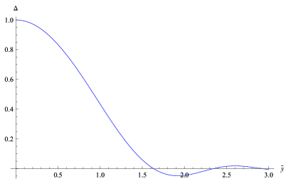
Figure 1: Dependence of the superconducting nucleus, $\Delta(\tilde{y})$, which is the solution of Eq.(34) at $\alpha=22.5^{0}$, on the coordinate $\tilde{y}$ (see Eq.(33)). We pay attention that $\Delta(\tilde{y})$ changes its sign in space.

To summarize, for the first time, we have suggested an adequate mathematical apparatus to calculate the four-fold anisotropy of the parallel upper critical magnetic field in Q2D $d$-wave superconductors at any temperatures and numerically have calculated its maximum value at $T=0$ in the absence of the paramagnetic effects. We stress that our theory has been elaborated for such Q2D superconductors [20], where $\xi_{\perp}\geq c^{*}$, with $\xi_{\perp}$ being perpendicular to the conducting layers coherent length and $c^{*}$ being the inter-layer distance. This is in contrast to the so-called Lawrence-Doniach model (see, for example, Refs.[21,22]). It is useful here to discuss more what we meant by writing $T=0$. First of all, we have considered a pure $d$-wave superconductor and, thus, we always meant that $\pi T_{c}\gg 1/\tau_{0}\rightarrow 0$. Secondly, we have suggested that $\pi T\gg\omega_{c}(H_{c2})$, which allows to disregard the quantum effects of electron motion in a magnetic field [11-13]. Note that the above mentioned quantum effects have been so far found to be important only for Q1D organic superconductors from chemical family (TMTSF)₂X (X=ClO${}_{4},$PF₆, etc.) [23].

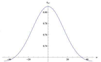
Figure 2: Angular dependence of the ratio $h_{c2}(\alpha)=H_{c2}(\alpha)/H^{GL}_{c2}(0)$, where $H_{c2}(\alpha)$ is the parallel upper critical magnetic field for the field in-plane direction (19) at $T=0$ and $H^{GL}_{c2}(0)$ is the Ginzburg-Landau parallel upper critical magnetic field (31) at $T=0$ (i.e., at $\tau$=1).

The author is thankful to N.N. Bagmet for useful discussions.

^∗Also at: L.D. Landau Institute for Theoretical Physics, RAS, 2 Kosygina Street, Moscow 117334, Russia.

References

• (1) C.C. Tsuei, J.R. Kirtley, C.C. Chi, et al., Phys. Rev. Lett. 73, 593 (1994).
• (2) Hyekyung Won, Kazumi Maki, Physica B 199-200, 353 (1994).
• (3) Kenji Takanaka and Kouichi Kuboya, Phys. Rev. Lett. 75, 323 (1995).
• (4) Takashi Sugiyama and Masanori Ichioka, J. Phys. Soc. Jpn. 67, 1738 (1998).
• (5) Y. Koyama, T. Sasagawa, Y. Togawa, et al., J. Low Temp. Phys. 117, 551 (1999).
• (6) See, for example, book A.A. Abrikosov, Fundamentals of Theory of Metals (Elsevier Science, Amsterdam, 1988).
• (7) Guangfeng Wang and Kazumi Maki, Phys. Rev. B 58, 6493 (1998).
• (8) F. Weickert, P. Gegenwart, H. Won, D. Parker, and K. Maki, Phys. Rev. B 74, 134511 (2006).
• (9) H.A. Viera, N. Oeschler, S. Seiro, H.S. Jeevan, C. Geibel, D. Parker, and F. Steglich, Phys. Rev. Lett. 106, 207001 (2011).
• (10) I.A. Luk’yanchuk and V.P. Mineev, Sov. Phys. JETP 66, 1168 (1987).
• (11) A.G. Lebed, JETP Lett. 44, 114 (1986) [Pis’ma Zh. Eksp. Teor. Fiz. 44, 89 (1986)].
• (12) N. Dupuis, G. Montambaux, and C.A.R. Sa de Melo, Phys. Rev. Lett. 70, 2613 (1993).
• (13) A.G. Lebed and K. Yamaji, Phys. Rev. Lett. 80, 2697 (1998).
• (14) L.P. Gor’kov, Sov. Phys. JETP, 37(10), 42 (1960).
• (15) A.A. Abrikosov, L.P. Gor’kov, and I.E. Dzyaloshinskii, Methods of Quantum Field Theory in Statistical Mechanics (Dover, New York, 1963).
• (16) L.P. Gor’kov and A.G. Lebed, J. Phys. (Paris) Lett. 45, L433 (1984).
• (17) V.P. Mineev and K.V. Samokhin, Introduction to Unconventional Superconductivity (Gordon and Breach Science Publisher, Australia, 1999).
• (18) I.S. Gradshteyn and I.M. Ryzhik, Table of Integrals, Series, and Products (6-th edition, Academic Press, London, United Kingdom, 2000).
• (19) L.P. Gor’kov and T.K. Melik-Barkhudarov, Zh. Eksp. Teor. Fiz. 45, 1493 (1963) [Sov. Phys. JETP 18, 1031 (1964).
• (20) A.G. Lebed, JETP Lett., 110, 173 (2019) [Pis’ma v Zh. Eksp. Teor. Fiz. 110, 163 (2019)].
• (21) L.N. Bulaevskii and A.A. Guseinov, Pis’ma Zh. Eksp. Teor. Fiz. 19, 742 (1974) [JETP Lett. 19, 382 (1974)].
• (22) R.A. Klemm, A. Luther, and M.R. Beasley, Phys. Rev. B 12, 877 (1975).
• (23) A.G. Lebed ed., The Physics of Organic Superconductors and Conductors (Springer-Verlag, Berlin, 2008).