Leveraging Class Hierarchies
with Metric-Guided Prototype Learning

Abstract

In many classification tasks, the set of target classes can be organized into a hierarchy. This structure induces a semantic distance between classes, and can be summarized under the form of a cost matrix, which defines a finite metric on the class set. In this paper, we propose to model the hierarchical class structure by integrating this metric in the supervision of a prototypical network. Our method relies on jointly learning a feature-extracting network and a set of class prototypes whose relative arrangement in the embedding space follows an hierarchical metric. We show that this approach allows for a consistent improvement of the error rate weighted by the cost matrix when compared to traditional methods and other prototype-based strategies. Furthermore, when the induced metric contains insight on the data structure, our method improves the overall precision as well. Experiments on four different public datasets—from agricultural time series classification to depth image semantic segmentation—validate our approach.

1 Introduction

Most classification models focus on maximizing the prediction accuracy, regardless of the semantic nature of errors. This can lead to high performing models, but puzzling errors such as confusing tigers and sofas, and casts doubt on what a model actually understands of the required task and data distribution. Neural networks in particular have been criticized for their tendency to produce improbable yet confident errors, notably when under adversarial attacks (?). Training deep models to produce not only produce fewer but also better errors can increase their trustworthiness, which is crucial for downstream applications such as autonomous driving or land use and land cover monitoring ??.

In many classification problems, the target classes can be organized according to a tree-shaped hierarchical structure. Such a taxonomy can be generated by domain experts, or automatically inferred from class names using the WordNet graph (?) or from word embeddings (?). A step towards more reliable and interpretable algorithms would be to explicitly model the difference of gravity between errors, as defined by a hierarchical nomenclature.

For a classification task over a set $\mathcal{K}$ of $K$ classes, the hierarchy of errors can be encapsulated by a cost matrix $D\in\mathbb{R}^{K\times K}_{+}$, defined such that the cost of predicting class $k$ when the true class is $l$ is $D[k,l]\geq 0$, and $D[k,k]=0$ for all $k=1\cdots K$. Among many other options (?), one can define $D[k,l]$ as the length of the shortest path between the nodes corresponding to classes $k$ and $l$ in the tree-shaped class taxonomy.

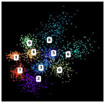
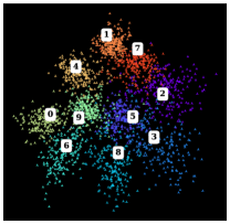
(a) Cross entropy,	(b) Learnt prototypes,	(c) Guided prototypes,
distortion${}^{1}=0.47$,	distortion$=0.42$,	distortion$=0.22$,
ER$=15.2\%$, AHC $=0.81$	ER$=14.2\%$, AHC $=0.75$	ER$=11.9\%$, AHC $=0.52$

Figure 1: Mean class representation , prototypes , and $2$-dimensional embeddings learnt on perturbed MNIST by a 3-layer convolutional net with three different classification modules: (a) cross-entropy, (b) learnt prototypes, and (c) learnt prototypes guided by a tree-shaped taxonomy (constructed according to the authors’ perceived visual similarity between digits). The guided prototypes (d) embed more faithfully the class hierarchy: classes with low error cost are closer. This is associated with a decrease in the Average Hierarchical Cost (AHC), as well as Error Rate (ER), indicating that our taxonomy may contain useful information for learning better visual features.

As pointed out by ?, the first step towards algorithms aware of hierarchical structures would be to generalize the use of cost-based metrics. For example, early iterations of the ImageNet challenge (??) proposed to weight errors according to hierarchy-based costs. For a dataset indexed by $\mathcal{N}$, the Average Hierarchical Cost (AHC) between class predictions $y\in\mathcal{K}^{\mathcal{N}}$ and the true labels $z\in\mathcal{K}^{\mathcal{N}}$ is defined as:

$$\text{AHC}(y,z)=\frac{1}{|\mathcal{N}|}\sum_{n\in\mathcal{N}}D[y_{n},z_{n}]~{}.$$ (1)

Along with the evaluation metrics, the loss functions should also take the cost matrix into account. While it is common to focus on retrieving certain classes through weighting ?? or sampling ?? schemes, preventing confusion between specific classes is less straightforward. For example, the cross entropy with one-hot target vectors singles out the predicted confidence for the true class, but treats all other classes equally. Beyond reducing the AHC, another advantage of incorporating the class hierarchy into the learning phase is that $D$ may contain information about the structure of the data as well. Although it is not always the case, co-hyponyms (i.e. siblings) in a class hierarchy tend to share some structural properties. Encouraging such classes to have similar representations could lead to more efficient learning, e.g. by leveraging common feature detectors. Such priors on the class structure may be especially crucial when dealing with a large taxonomy, as noted by ?.

In this paper, we introduce a method to integrate a pre-defined class hierarchy into a classification algorithm. We propose a new distortion-based regularizer for prototypical network (??). This penalty allows the network to learn prototypes organized so that their pairwise distances reflect the error cost defined by a class hierarchy. Our contributions are as follows:

• We introduce a scale-independent formulation of the distortion between two metric spaces and an associated smooth regularizer.

• This formulation allows us to incorporate knowledge of the class hierarchy into a neural network at no extra cost in trainable parameters and computation.

• We show on four public datasets (CIFAR100 , NYUDv2, S2-Agri, and iNaturalist-19) that our approach decreases the average cost of the prediction of standard backbones.

• As illustrated in Figure 1, we show that our approach can also lead to a better (unweighted) precision, which we attribute to the useful priors contained in the hierarchy.

2 Related Work

Prototypical Networks:

Our approach builds on the growing corpus of work on prototypical networks. These models are deep learning analogues of nearest centroid classifiers (?) and Learning Vector Quantization networks (??), which associate to each class a representation, or prototype, and classify the observations according to the nearest prototype. These networks have been successfully used for few-shot learning (??), zero-shot learning (?), and supervized classification (????).

In most approaches, the prototypes are directly defined as the centroid of the learnt representations of samples of their classes, and updated at each episode (?) or iteration (?). In the work of ? and ?, the prototypes are defined prior to learning the embedding function. In this work, we follow the approach of ? and learn the prototypes simultaneously with the data embedding function.

Hierarchical Priors:

The idea of exploiting the latent taxonomic structure of semantic classes to improve the accuracy of a model has been extensively explored (?), from traditional Bayesian modeling (?, Chapter 5) to adaptive deep learning architectures (????). However, for these neural networks, the hierarchy is discovered by the network itself to improve the overall accuracy of the model. In our setting, the hierarchy is defined a priori and serves both to evaluate the quality of the model and to guide the learning process towards a reduced prediction cost.

? propose to implement Gaussian priors on the weight of neurons according to a fixed hierarchy. ? implements an inference scheme based on a tree-shaped graphical model derived from a class taxonomy. Closest to our work, ? propose a regularization based on the earth mover distance to penalize errors with high cost.

More recently, ? highlighted the relative lack of well-suited methods for dealing with hierarchical nomenclatures in the deep learning literature. They advocate for a more widespread use of the AHC for evaluating models, and detail two simple baseline classification modules able to decrease the AHC of deep models: Soft-Labels and Hierarchical Cross-Entropy. See the appendix for more details on these schemes. Following this objective, ? propose a an inference-time risk minimization scheme to reduce the AHC of the predictions based on the predicted posteriors.

Hyperbolic Prototypes:

Motivated by their capacity to embed hierarchical data structures into low-dimensional spaces, (?), hyperbolic spaces are at the center of recent advances in modeling hierarchical relations (??). Closer to this work, (??) also propose to embed a class hierarchy into the latent representation space. However, both approaches embed the class hierarchy before training the data embedding network. In contrast, we argue that incorporating the hierarchical structure during the training of the model allows the network and class embeddings to share their respective insights, leading to a better trade-off between AHC and accuracy. In this paper, we only explore Euclidean geometry, as this setting allows for the seamless integration of our method without changing the number of bits of precision or the optimizer ?.

Finite Metric Embeddings:

Our objective of computing class representations with pairwise distances determined by a cost matrix has links with finding an isometric embedding of the cost matrix—seen as a finite metric. This problem has been extensively studied (??) and is at the center of the growing interest for hyperbolic geometry (?). Here, our goal is simply to influence the learning of prototypes with a metric rather than necessarily seeking the best possible isometry.

3 Method

We consider a generic dataset $\mathcal{N}$ of $N$ elements $x\in\mathcal{X}^{\mathcal{N}}$ with ground truth classes $z\in\mathcal{K}^{\mathcal{N}}$. The classes $\mathcal{K}$ are organized along a tree-shape hierarchical structure, allowing us to define a cost matrix $D$ by considering the shortest path between nodes. The matrix thus defined is symmetric, with a zero diagonal, strictly positive elsewhere, and respects the triangle inequality: $D[k,l]+D[l,m]\geq D[k,m]$ for all $k,l,m$ in $\mathcal{K}$. In other words, $D$ defines a finite metric. We denote by $\Omega$ an embedding space which, when equipped with the distance function $d:\Omega\times\Omega\mapsto\mathbb{R}_{+}$, forms a continuous metric space.

3.1 Prototypical Networks

A prototypical network is characterized by an embedding function $f:\mathcal{X}\mapsto\Omega$, typically a neural network, and a set $\pi\in\Omega^{\mathcal{K}}$ of $K$ prototypes. $\pi$ must be chosen such that any sample $x_{n}$ of true class $k$ has a representation $f(x_{n})$ which is close to $\pi_{k}$ and far from other prototypes.

Following the methodology of ?, a prototypical network $(f,\pi)$ associates to an observation $x_{n}$ the posterior probability over its class $z_{n}$ defined as follows:

$$p(z_{n}=k|x_{n}) =\frac{\exp{\left(-d\left(f(x_{n}),\pi_{k}\right)\right)}}{\sum_{l\in\mathcal{K}}\exp{\left(-d\left(f(x_{n}),\pi_{l}\right)\right)}}~{},\forall k\in\mathcal{K}$$ (2)

We define an associated loss as the normalized negative log-likelihood of the true classes:

$$\mathcal{L}_{\text{data}}(f,\pi) =\frac{1}{N}\sum_{n\in\mathcal{N}}\left(d(f(x_{n}),\pi_{z_{n}})+\log\left(\sum_{l\in\mathcal{K}}\exp{(-d(f(x_{n}),\pi_{l}))}\right)\right)~{}.$$ (3)

This loss encourages the representation $f(x_{n})$ to be close to the prototype of the class $z_{n}$ and far from the other prototypes. Conversely, the prototype $\pi_{k}$ is drawn towards the representations $f(x_{n})$ of samples $n$ with true class $k$, and away from the representations of samples of other classes.

Following the insights of ?, the embedding function $f$ and the prototypes $\pi$ are learned simultaneously. This differs from many works on prototypical networks which learn prototypes separately or define them as centroids of representations. We take advantage of this joint training to learn prototypes which take into account both the distribution of the data and the relationships between classes, as described in the next section.

3.2 Metric-Guided Penalization

We propose to incorporate the cost matrix $D$ into a regularization term in order to encourage the prototypes’ positions in the embedding space $\Omega$ to be consistent with the finite metric defined by $D$. Since the sample representations are attracted to their respective prototypes in (3), such regularization will also affect the embedding network.

Metric Distortion

As described in ?, the distortion of a mapping $k\mapsto\pi_{k}$ between the finite metric space $(\mathcal{K},D)$ and the continuous metric space $(\Omega,d)$ can be defined as the average relative difference between distances in the source and target space:

$$\text{disto}(\pi,D) =\frac{1}{K(K-1)}\sum_{k,l\in\mathcal{K}^{2},\,k\neq l}\frac{\left|d(\pi_{k},\pi_{l})-D[k,l]\right|}{D[k,l]}~{}.$$ (4)

We argue that a network $(f,\pi)$ trained to minimize $\mathcal{L}_{\text{data}}$ and whose prototypes $\pi$ have a low distortion with respect to $D$ should produce errors with low hierarchical costs. To understand the intuition behind this idea, let us consider a sample $x_{n}$ of true class $k$ and misclassified as class $l$. This tells us that the distance between $f(x_{n})$ and $\pi_{l}$ is small. If $k$ and $l$ have a high cost according to $D$, and since $k\mapsto\pi_{k}$ is of low distortion, then $d(\pi_{k},\pi_{l})$ must be large. The triangular inequality tells us that $d(f(x_{n}),\pi_{k})\geq d(\pi_{k},\pi_{l})-d(f(x_{n}),\pi_{l})$, and consequently that $d(f(x_{n}),\pi_{k})$ must be large as well, which contradicts that $(f,\pi)$ minimizes $\mathcal{L}_{\text{data}}$.

Scale-Free Distortion

For a prototype arrangement $\pi$ to have a small distortion with respect to a finite metric $D$ as defined in Equation 4, the distance between prototypes must correspond to the distance between classes. This imposes a specific scale on the distances between prototypes in the embedding space. This scale may conflict with the second term of $\mathcal{L}_{\text{data}}$ which encourages the distance between embeddings and unrelated prototypes to be as large as possible. Therefore, lower distortion may also cause lower precision. To remove this conflicting incentive, we introduce a scale-independent formulation of the distortion (5) where $s\cdot\pi$ are the scaled prototypes, whose coordinates in $\Omega$ are multiplied by a scalar factor $s$. As shown in the appendix, $\text{disto}^{\text{scale-free}}$ can be efficiently computed algorithmically.

$$\text{disto}^{\text{scale-free}}(\pi,D) =\min_{s\in\mathbb{R}_{+}}{\text{disto}(s\cdot\pi,D)}~{},$$ (5)

Distortion-Based Penalization

We propose to incorporate the error qualification $D$ into the prototypes’ relative arrangement by encouraging a low scale-free distortion between $\pi$ and $D$. To this end, we define $\mathcal{L}_{\text{disto}}$, a smooth surrogate of $\text{disto}^{\text{scale-free}}$ (6). as detailed in the appendix, $\mathcal{L}_{\text{disto}}$ can be computed in closed form as a function of $\pi$ and can be directly used as a regularizer.

$$\mathcal{L}_{\text{disto}}(\pi) =\frac{1}{K(K-1)}\min_{s\in\mathbb{R}_{+}}\sum_{k,l\in\mathcal{K}^{2},\,k\neq l}\left(\frac{sd(\pi_{k},\pi_{l})-D[k,l]}{D[k,l]}\right)^{2}~{}.$$ (6)

3.3 End-to-end Training

We combine $\mathcal{L}_{\text{data}}$ and $\mathcal{L}_{\text{disto}}$ in a single loss $\mathcal{L}$. $\mathcal{L}_{\text{data}}$ allows to jointly learn the embedding function $f$ and the class prototypes $\pi$, while $\mathcal{L}_{\text{disto}}$ enforces a metric-consistent prototype arrangement, with $\lambda\in\mathbb{R}_{+}$ an hyper-parameter setting the strength of the regularization:

$$\mathcal{L}(f,\pi)=\mathcal{L}_{\text{data}}(f,\pi)+\lambda\mathcal{L}_{\text{disto}}(\pi)~{}.$$ (7)

4 Experiments

4.1 Datasets and Backbones

Table 1: Data composition and taxonomies of the four studied datasets. IR stands for the Imbalance Ratio (largest over smallest class count), nodes and leaves denote respectively the total number of classes and leaf-classes in the tree-shape hierarchy, ABF stands for the Average Branching Factor, and $\langle D\rangle$ stands for the average pairwise distance.

Dataset	Data				Hierarchical Tree
	Volume (Gb)	Samples	IR		Depth	Nodes (leaves)	ABF	$\langle D\rangle$
NYUDv2	2.8	1449	93		3	57 (40)	5.0	4.3
S2-Agri	28.2	189 971	617		4	83 (45)	5.8	6.5
CIFAR100	0.2	60 000	1		5	134 (100)	3.8	7.0
iNat-19	82.0	265 213	31		7	1189 (1010)	6.6	11.0

We evaluate our approach with different tasks and public datasets with fine-grained class hierarchies: image classification on CIFAR100 (?) and iNaturalist-19 (?), RGB-D image segmentation on NYUDv2 (?), and image sequence classification on S2-Agri (?). We define the cost matrix of these class sets as the length of the shortest path between nodes in the associated tree-shape taxonomies represented in the Appendix. As shown in Table 1, these datasets cover different settings in terms of data distribution and hierarchical structure.

Illustrative Example on MNIST:

In Figure 1, we illustrate the difference in performance and embedding organization of the embedding space for different approaches. We use a small 3-layer convolutional net trained on MNIST with random rotations (up to $40$ degrees) and affine transformations (up to $1.3$ scaling). For plotting convenience, we set the features’ dimension to $2$.

Image Classification on CIFAR100:

We use a super-class system inspired by ? and form a $5$-level hierarchical nomenclature of size: $2$, $4$, $8$, $20$, and $100$ classes. We use as backbone the established ResNet-18 (?) as embedding network for this dataset.

RGB-D Semantic Segmentation on NYUDv2:

We use the standard split of $795$ training and $654$ testing pairs. We combine the $4$ and $40$ class nomenclatures of ? and the $13$ class system defined by ? to construct a $3$-level hierarchy. We use FuseNet (?) as backbone for this dataset.

Image Sequence Classification on S2-Agri:

S2-Agri is composed of $189\;971$ sequences of multi-spectral satellite images of agricultural parcels. We define a $4$-level crop type hierarchy of size $4$, $12$, $19$, and $44$ classes with the help of experts from a European agricultural monitoring agency (ASP). We use the PSE+TAE architecture (?) as backbone, and follow their $5$-fold cross-validation scheme for training. Crop mapping in particular benefits from predictions with a low hierarchical cost. Indeed, payment agencies monitor the allocation of agricultural subsidies and whether crop rotations follow best practice recommendations ?. The monetary and environmental impact of misclassifications are typically reflected in the class hierarchy designed by domain experts ??. By achieving a low AHC, we ensure that these downstream tasks can be meaningfully realized from the predictions.

Fine-Grained Image Classification on iNaturalist-19 (iNat-19)

iNat-19 (?) contains $1\,010$ different classes organized into a $7$ level hierarchy with respective width $3$, $4$, $9$, $34$, $57$, $72$, and $1\,010$. We use ResNet-18 pretrained on ImageNet as backbone. We sample $75\%$ of available images for training, while the rest is evenly split into a validation and test set.

4.2 Hyper-Parameterization

The embedding space $\Omega$ is chosen as $\mathbb{R}^{512}$ for iNat-19 and $\mathbb{R}^{64}$ for all other datasets. We chose $d$ as the Euclidean norm. (see 4.6 for a discussion on this choice). We evaluate our approach (Guided-proto) with $\lambda=1$ in (7) for all datasets. We use the same training schedules and learning rates as the backbone networks in their respective papers. In particular, the class imbalance of S2-Agri is handled with a focal loss (?).

4.3 Competing methods

In the paper where they are introduced, all backbone networks presented in Section 1 use a linear mapping between the sample representation and the class scores, as well as the cross-entropy loss. The resulting performance defines a baseline, denoted as Cross-Entropy, and is used to estimate the gains in Average Hierarchical Cost (AHC) and Error Rate (ER) provided by different approaches. We reimplemented other competing methods: Hierarchical Cross-Entropy (HXE) ?, Soft Labels ?, Earth Mover Distance regularization (XE+EMD) ?, Hierarchical Inference (YOLO) ?, Hyperspherical Prototypes (Hyperspherical-proto) ?, and Deep Mean Classifiers (Deep-NCM) ?. See the Appendix for more details on these methods. Lastly, we evaluate simple prototype learning (Learnt-proto) ? by setting $\lambda=0$ in (7).

4.4 Analysis

Figure 2: Error Rate (ER) in % and Average Hierarchical Cost (AHC) on four datasets for Guided-proto, the Cross-Entropy baseline (in bold), and competing approaches. Methods that use the hierarchical knowledge are indicated with the symbol . The best performances on each dataset are plotted in green. Our guided prototype approach improves both the ER and AHC across the four datasets compared to the baseline. The metrics are computed with the median over $5$ runs for CIFAR100, the average over $5$ cross-validation folds for S2-Agri, and a single run for NYUDv2 and iNat-19. The numeric values are given in the Appendix. ($\star$: not evaluated).

Overall Performance:

As displayed in Figure 2, the benefits provided by our approach can be appreciated on all datasets. Compared to the Cross-Entropy baseline, our model improves the AHC by $3\%$ on NYUDv2 and S2-Agri, and up to $9$% and $14$% for CIFAR100, and iNat-19 respectively. The hierarchical inference scheme YOLO of ? performs on par or better than our methods for NYUDv2 and S2-Agri, while Soft-labels perform well on CIFAR100 and NYUDv2. Yet, metric guided prototypes brings the most consistent reduction of the hierarchical cost across all tasks, datasets, and class hierarchies configurations. This suggest that arranging the embedding space consistently with the cost metric is a robust way of reducing a model’s hierarchical error cost. We argue that these results, combined with its ease of implementation, make a strong case for our approach.

While being initially designed to reduce the AHC, our method also provides a relative decrease of the ER by $3$ to $4$% across all datasets compared to the cross-entropy baseline. This indicates that cost matrices derived from the class hierarchies can indeed help neural networks to learn richer representations.

Prototype Learning:

We observe that the learnt prototype approach Learnt-proto consistently outperforms the Deep-NCM method. This suggests that defining prototypes as the centroids of their class representations might actually be disadvantageous. As illustrated on Figure 1, the positions of the embeddings tend to follow a Voronoi partition (?) with respect to the learnt prototypes of their true class rather than prototypes being the centroid of their associated representations. A surprising observation for us is that Learnt-proto consistently outperforms the Cross-Entropy baseline, both in terms of AHC and ER.

Computational Efficiency:

Computing distances between representations and prototypes is comparable in terms of complexity than computing a linear mapping. The scaling factor in $\mathcal{L}_{\text{disto}}$ can be efficiently obtained as described in the Appendix. In practice, we observed that both training and inference time are identical for Cross-Entropy and Guided-proto: most of the time is taken by the computation of the embeddings.

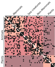
(a) Cross-Entropy

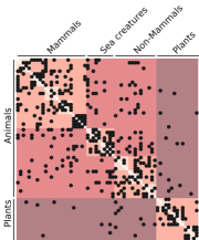
(b) Metric-Guided Prototypes

(c) Hierarchical cost

Figure 3: Partial confusion matrix for the “living organism” class subset of CIFAR100 for the Cross-Entropy baseline (a) and our approach (b). For readability, we only display (in black) entries of the matrices with at least one confusion. We also represent the cost of confusing different classes in shades of reds (c). We note that our approach yields fewer confusions between pairs of classes with high costs, such as plants and animals.

4.5 Restricted Training Data Regime

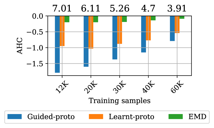
Figure 4: AHC of ResNet-18 trained on restricted training sets of iNaturalist-19 with Guided-proto, Learnt-proto, and EMD. We represent the relative improvement compared to the performance of the Cross-Entropy baseline, which is shown on top of the plots.

We observed that the Learnt-proto method decreases the AHC across all four datasets even though it does not take the cost matrix into account. This suggests that, given enough data, this simple model can learn an empirical taxonomy through its prototypes’ arrangement. Furthermore, this taxonomy can share enough similarity with the one designed by experts to result in a decrease in AHC. To further evaluate the benefit of explicitly using the expert taxonomy with our approach, we train the models Learnt-proto, Guided-proto, and EMD with only part of the $160$k images in the training set of iNat-19, and without pretraining on ImageNet. To compensate for the lack of data, we increase the regularization strength to $\lambda=20$.

In Figure 4, we observe that the two prototype-based approaches consistently improve the performance of the baseline for all training set sizes in terms of AHC. Moreover, the advantages brought by our proposed regularization are all the more significant when applied to small training sets. This observation reinforces the idea that the learnt-proto method requires large amounts of data to learn a meaningful class hierarchy in an unsupervized way.

4.6 Ablation Study

In the Appendix, we present an extensive ablation study. We present here its main take-away.

Scale-Free Distortion:

Our method for automatically choosing the best scale in our smooth distortion surrogate leads to an improvement of $0.9$ ER on the iNat-19 dataset, which amounts to half the improvement compared to the baseline. In the other datasets, the improvements were more limited. We attribute the impact of our scale-free distortion on iNat-19 in particular to the structure of its class hierarchy: at the lowest level, iNat-19 classes have on average $14$ co-hyponyms (siblings), compared to only $2$ to $5$ for the other datasets. When minimizing the distortion with a fixed scale of $1$, the prototypes of hyponyms are incentivized to be close with respect to $d$ since hyponyms have a small hierarchical distance of $2$. This clashes with the minimization of the second part of $\mathcal{L}_{\text{data}}$ as defined in $(\hyperref@@ii[eq:ldata_long]{\ref*{eq:ldata_long}})$, which mutually repels prototypes of different classes. This conflict, made worse by classes with many hyponyms, is removed by our scale-free distortion. See the Appendix for additional insights into how our automatic scaling addresses this issue.

Choice of Metric Space:

Prototypical networks operating on $\Omega=\mathbb{R}^{m}$ typically use the squared Euclidean norm in the distance function, motivated by its quality as a Bregman divergence (?). However, given the large distance between prototypes induced by our regularization, this metric can cause stability issues. We observe for all datasets that that defining $d$ as the Euclidean norm yields significantly better results across all datasets.

Guided vs. fixed prototypes :

As suggested by the lower performance of Hypersphe- rical-proto, jointly learning the prototypes and the embedding network can be advantageous. To confirm this observation, we altered our Guided-proto method to first learn the prototypes and then the embedding network. We observed a significant decrease in performance across the board, up to $5$ more points of ER in iNat-19. Conversely, we altered Hyperspherical-proto to learn spherical prototypes together with the embedding network. This improved the performance of Hyperspherical-proto even though it remained worse than the Cross-Entropy baseline ($+1.20$ ER, $+0.10$ AHC on CIFAR100). These observations suggest that insights from the data distribution can benefit the positioning of prototypes, and that they should be learned conjointly.

5 Conclusion

We introduced a new regularizer modeling the hierarchical relationships between the classes of a nomenclature. This approach can be incorporated into any classification network at no computational cost and with very little added code. We showed that our method consistently decreased the average hierarchical cost of three different backbone networks on different tasks and four datasets. Furthermore, our approach can reduce the rate of errors as well. In contrast to most recent works on hierarchical classification, we showed that this joint training is beneficial compared to the staged strategy of first positioning the prototypes and then training a feature extracting network. A PyTorch implementation of our framework as well as an illustrative notebook are available at https://github.com/VSainteuf/metric-guided-prototypes-pytorch.

Supplementary Materials - Leveraging Class Hierarchies with Metric-Guided Prototype Learning

6 Notebook and illustration

In Figure 5, we represent the embeddings and prototypes generated by variations of our networks as well as their respective performance. We note that the fixed prototypes approach performs significantly worse than our metric-guided method. We observe that the resulting prototypes are more compact when they are learned independently, which can lead to an increase in misclassification. We also remark that when the hierarchy contains no useful information, such as the arbitrary order of digits, the metric-based approach has a worse performance than the free (unguided) method. This is particularly drastic for the fixed prototype approach.

An illustrated notebook to reproduce this figure can be accessed at the following URL:

https://colab.research.google.com/drive/1VoQfBx5q5lWFev0cwxLZ0qQOZU7Rlmb_#offline=true&sandboxMode=true

To run this notebook locally, you can also download it from our repository:
https://github.com/VSainteuf/metric-guided-prototypes-pytorch.

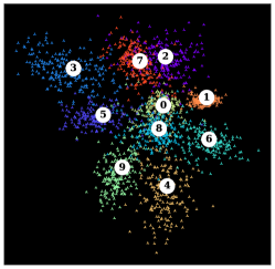
(a) Cross entropy, ER$=15.2\%$ disto${}_{\text{vis}}=0.47$, disto${}_{\text{abs}}=0.61$ AHC${}_{\text{vis}}=0.81$, AHC${}_{\text{abs}}=0.65$

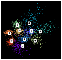
(b) Learnt prototypes, ER$=14.2\%$ disto${}_{\text{vis}}=0.42$, disto${}_{\text{abs}}=0.58$ AHC${}_{\text{vis}}=0.75$, AHC${}_{\text{abs}}=0.50$

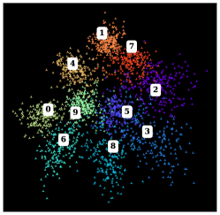
(c) Guided prototypes, ER$=12.8\%$ disto${}_{\text{vis}}=0.22$ AHC${}_{\text{vis}}=0.56$

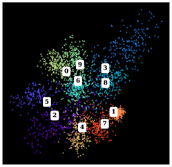
(d) Fixed prototypes, ER$=21.5\%$ disto${}_{\text{vis}}=0.17$ AHC${}_{\text{vis}}=0.82$

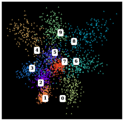
(e) Guided prototypes, ER$=16.9\%$ disto${}_{\text{abs}}=0.24$ AHC${}_{\text{abs}}=0.54$

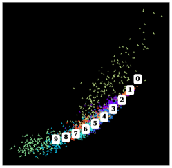
(f) Fixed prototypes, ER$=48.8\%$ disto${}_{\text{abs}}=0.00$ AHC${}_{\text{abs}}=0.80$

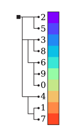
Figure 5: Mean class representation , prototypes , and $2$-dimensional embeddings learnt on perturbed MNIST by a 3-layer convolutional net with six different classification modules: (a) cross-entropy, (b) learnt prototypes, (c) learnt prototypes guided by a visual taxonomy, (d) fixed prototypes (see Section 8.2) from a visual taxonomy , (e) learnt prototypes guided by the numbers’ values, and (f) fixed prototypes from the numbers’ values. The visual hierarchy is represented in (g) and the numerical order in (h). AHC${}_{\text{vis}}$ corresponds to the cost defined by our proposed visual hierarchy, while AHC${}_{\text{abs}}$ is defined after the chain-like structure obtained when organizing the digits along their numerical values. While embedding the metric with prototypes prior to learning the representations leads to lower (scale-free) distortion, this translates into worst performance in terms of AHC and ER. Joint learning achieves better performance on both evaluation metrics. We also remark that when the hierarchy is arbitrary (e-f), metric guiding is detrimental to precision.

7 Additional methodological details

7.1 Scale-Independent Distortion

Computing the scale-free distortion defined in Equation 5 amounts to finding a minimizer of the following function $f:\mathbb{R}\mapsto\mathbb{R}$:

$$f(s) =\sum_{i\in I}\left|s\alpha_{i}-1\right|,$$ (8)

with $\alpha_{k,l}=d(\pi_{k},\pi_{l})/D[k,l]\geq 0$, and $I$ an ordering of $\{k,l\}_{k,l\in\mathcal{K}^{2}}$ such that the sequence $[\alpha_{i}]_{i\in I}$ is non-decreasing.

Proposition 1.

A global minimizer of $f$ defined in (8) is given by $s^{\star}=1/\alpha_{k^{\star}}$ with $k^{\star}$ defined as:

$$k^{\star}=\min\left\{k\in I\,\middle|\,\sum_{i\leq k}\alpha_{i}\geq\sum_{i>k}\alpha_{i}~{}.\right\}$$ (9)

Proof.

First, such $k^{\star}$ exists as it is the smallest member of a discrete, non-empty set. Indeed, since all $\alpha_{i}$ are nonnegative, the set contains at least $k=|I|$. We now verify that $s^{\star}=1/\alpha_{k}^{\star}$ is a critical point of $f$. By definition of $k^{\star}$ we have that $\sum_{i\leq k^{\star}}\alpha_{i}\geq\sum_{i>k^{\star}}\alpha_{i}$ and $\sum_{i<k^{\star}}\alpha_{i}<\sum_{i\geq k^{\star}}\alpha_{i}$. By combining these two inequalities, we have that

$$-\sum_{i<k^{\star}}\alpha_{i}+\sum_{i>k^{\star}}\alpha_{i} \in[-\alpha_{k^{\star}},\alpha_{k^{\star}}]~{}.$$ (10)

Since $I$ orders the $\alpha_{i}$ in increasing order, we can write the subgradient of $f$ at $s^{\star}$ under the following form:

$$\partial_{s}f(s^{\star}) =\sum_{i<k^{\star}}\partial_{s}\left|s^{\star}\alpha_{i}-1\right|+\sum_{i>k^{\star}}\partial_{s}\left|s^{\star}\alpha_{i}-1\right|+\partial_{s}\left|s^{\star}\alpha_{k^{\star}}-1\right|$$ (11)

$$=-\sum_{i<k^{\star}}\alpha_{i}+\sum_{i>k^{\star}}\alpha_{i}+[-\alpha_{k^{\star}},\alpha_{k^{\star}}].$$ (12)

By using the inequality defined in Equation 10, we have that $0\in\partial_{s}f(s^{\star})$ and hence $s^{\star}$ is a critical point of $f$. Since $f$ is convex, such $s^{\star}$ is also a global minimizer of $f$, i.e. an optimal scaling. ∎

This proposition gives us a fast algorithm to obtain an optimal scaling and hence a scale-free distortion: compute the cumulative sum of the $\alpha_{k,l}$ sorted in ascending order until the equality in (9) is first verified at index $k^{\star}$. The resulting optimal scaling is then given by $1/\alpha_{k^{\star}}$.

7.2 Smooth Distortion

The minimization problem with respect to $s$ defined in Equation 6 can be solved in closed form:

$$s^{\star} ={\sum\frac{d(\pi_{k},\pi_{l})}{D[k,l]}}\bigg{/}{\sum\frac{d(\pi_{k},\pi_{l})^{2}}{D[k,l]^{2}}}~{}.$$ (13)

7.3 Evolution of Optimal Scaling

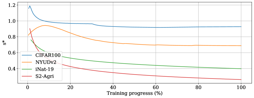
Figure 6: Evolution of the scaling factor $s^{*}$ in $\mathcal{L}_{\text{disto}}$ along the training iterations of the four networks. We observe that $s^{*}$ consistently decreases to values smaller than $1$, which allow the prototypes to spread apart while respecting the fix distances defined by $D$.

In Figure 6, we represent the evolution of the scaling factor $s^{*}$ in $\mathcal{L}_{\text{disto}}$ during training of our guided prototype method on the four datasets. Across all four models, $s^{*}$ presents a decreasing trend overall, which signifies that the average distance between prototypes increases. This is consistent with our analysis of prototypical networks: as the feature learning network and the prototypes are jointly learned, the samples’ representations get closer to their true class’ prototype. In doing so, they repel the other prototypes, which translate into an inflation of the global scale of the problem. Our optimal scaling allows the prototypes’ scale to expand accordingly. Without adaptive scaling, the data loss (3) and regularizer (6) would conflict.

In all our experiments, this scale remained bounded and did not diverge. This can be explained by the fact that for each misclassification $k\rightarrow l$ of a sample $x_{n}$, the representation $f(x_{n})$ is by definition closer to the erroneous prototype $\pi_{l}$ than of the true prototype $\pi_{k}$. The first term of $\mathcal{L}_{\text{data}}$ pushes the true prototype $\pi_{k}$ towards $f(x_{n})$, and by transitivity—towards the erroneous prototype $\pi_{l}$. This phenomenon prevents prototypes from being pushed away from one another indefinitely. However, if the prediction is too precise, i.e. most samples are correctly classified, the prototypes may diverge. This setting, which we haven’t yet encountered, may necessitate a regularization such as weight decay on the prototypes parameters.

Lastly, we remark that the asymptotic optimal scalings are different from one dataset to another. This can be explained foremost by differences in the depth and density of the class hierarchy of each dataset, as presented in Table 1. As explained above, the inherent difficulty of the classification tasks also have an influence on the problem’s scale. However, our parameter-free method is able to automatically find an optimal scaling.

7.4 Inference

As with other prototypical networks, we associate to a sample $n$ the class $k$ whose prototype $\pi_{k}$ is the closest to the representation $f(x_{n})$ with respect to $d$, corresponding to the class of highest probability. This process can be made efficient for a large number of classes $K$ and a high embedding dimension $m$ with a KD-tree data structure, which offers a query complexity of $O(\log(K))$ instead of $O(K\cdot m)$ for an exhaustive comparison. Hence, our method does not induce longer inference time than the cross-entropy for example, as the embedding function typically takes up the most time.

7.5 Rank-based Guiding

Following the ideas of ?, we also experiment with a RankNet-inspired loss (?) which encourages the distances between prototypes to follow the same order as the costs between their respective classes, without imposing a specific scaling:

$$\mathcal{L}_{\text{rank}}(\pi) =-\frac{1}{|\mathcal{T}|}\sum_{k,l,m\in\mathcal{T}}\bar{\bf R}_{k,l,m}\cdot\text{log}(R_{k,l,m})+(1-\bar{\bf R}_{k,l,m})\cdot\text{log}(1-R_{k,l,m})~{},$$ (14)

with $\mathcal{T}=\{(k,l,m)\in\mathcal{K}^{3}\mid k\neq l,l\neq m,k\neq m\}$ the set of ordered triplet of $\mathcal{K}$, $\bar{\bf R}_{k,l,m}$ the hard ranking of the costs between $D_{k,l}$ and $D_{k,m}$, equal to $1$ if $D_{k,l}>D_{k,m}$ and $0$ otherwise, and $R_{k,l,m}=\text{sigmoid}(d(\pi_{k},\pi_{l})-d(\pi_{k},\pi_{m}))$ the soft ranking between $d(\pi_{k},\pi_{l})$ and $d(\pi_{k},\pi_{m})$. For efficiency reasons, we sample at each iteration only a $S$-sized subset of $\mathcal{T}$. We use $S=10$ in our experiments.

8 Additional experimental details

We give additional details on our experiments and some supplementary results in the following subsections.

8.1 Competing methods

Hierarchical Cross-Entropy

(HXE) ? model the class structure with a hierarchical loss composed of the sum of the cross-entropies at each level of the class hierarchy. As suggested, a parameter $\alpha$ taken as $0.1$ defines exponentially decaying weights for higher levels.

Soft Labels

(Soft-labels) ? propose as second baseline in which the the one-hot target vectors are replaced by soft target vectors in the cross-entropy loss. These target vectors are defined as the softmin of the costs between all labels and the true label, with a temperature ${1}/{\beta}$ chosen as $0.1$, as recommended in ?.

Earth Mover Distance regularization

(XE+EMD): ? propose to account for the relationships between classes with a regularization based on the squared earth mover distance. We use $D$ as the ground distance matrix between the probabilistic prediction $p$ and the true class $y$. This regularizer is added along the cross-entropy with a weight of $0.5$ and an offset $\mu$ of $3$.

Hierarchical Inference

(YOLO): ? propose to model the hierarchical structure between classes into a tree-shaped graphical model. First, the conditional probability that a sample belongs to a class given its parent class is obtained with a softmax restricted to the class’ co-hyponyms (i.e. siblings). Then, the posterior probability of a leaf class is given by the product of the conditional probability of its ancestors. The loss is defined as the cross-entropy of the resulting probability of the leaf-classes.

Hyperspherical Prototypes

(Hyperspherical-proto): The method proposed by ? is closer to ours, as it relies on embedding class prototypes. They advocate to first position prototypes on the hypersphere using a rank-based loss (see Section 4.6) combined with a prototype-separating term. They then use the squared cosine distance between the image embeddings and prototypes to train the embedding network. Note that in our re-implementation, we used the finite metric defined by $D$ instead of Word2Vec (?) embeddings to position prototypes. Lastly, we do not evaluate on S2-Agri as the integration of the focal loss is non-trivial.

Deep Mean Classifiers

(Deep-NCM): ? present another prototype-based approach. Here, the prototypes are the cumulative mean of the embeddings of the classes’ samples, updated at each iteration. The embedding network is supervised with $\mathcal{L}_{\text{data}}$ with $d$ defined as the squared Euclidean norm.

8.2 Numerical results

The numerical values of the results shown in Figure 2 are given in Table 2.

————————————————————-

(a) Porcupine $\leftrightarrow$ Shrew $-80\%$, $D_{a}=4$

(b) Caterpillar $\leftrightarrow$ Lizard $-64\%$, $D_{b}=4$

(c) Plate $\leftrightarrow$ Clock $-40\%$, $D_{c}=4$

(d) Streetcar $\leftrightarrow$ Bus $+58\%$, $D_{d}=4$

(e) Otter $\leftrightarrow$ Seal $+60\%$, $D_{e}=2$

(f) Boy $\leftrightarrow$ Man $+78\%$, $D_{f}=2$

Figure 7: Best (a-c) and worse (d-f) improvements in terms of class confusion provided by Guided-proto compared to the cross-entropy baseline for CIFAR100, given in $\%$, along with their error cost. The metric guided regularization particularly helps decreasing the confusions between classes that are visually similar (e.g. Plate and Clock) but are not direct siblings in the class hierarchy ($D=4$). Conversely, the regularization hinders performance for visually similar siblings classes (e.g. Otter and Seal, $D=2$).

Table 2: Error Rate (ER) in % and Average Hierarchical Cost (AHC) on three datasets for our proposed methods (top) and the competing approaches (bottom). The values are computed with the median over $5$ runs for CIFAR100, the average over $5$ cross-validation folds for S2-Agri, and a single run for NYUDv2 and iNat-19. (HSP: Hyperspherical Prototypes, GP: Guided Prototypes).

	CIFAR100			NYUDv2			S2-Agri			iNat-19
	ER	AHC		ER	AHC		ER	AHC		ER	AHC
Cross-Entropy	24.2	1.160		32.7	1.486		19.4	0.699		40.9	1.993
HXE	24.1	1.168		32.4	1.456		19.5	0.731		41.8	2.013
Soft-label	23.5	1.046		32.4	1.424		19.2	0.703		52.8	2.029
XE+EMD	24.5	1.196		33.3	1.498		19.0	0.687		40.1	1.893
YOLO	26.2	1.214		32.0	1.425		19.1	0.685		42.0	1.942
HSP	29.4	1.472		49.7	2.329		-	-		42.4	2.027
Deep-NCM	25.6	1.249		33.5	1.498		19.4	0.702		40.8	1.929
Free-proto	23.8	1.091		32.5	1.462		19.1	0.691		38.8	1.728
Fixed-proto	24.7	1.083		33.1	1.462		19.4	0.710		43.9	2.148
GP-rank	23.3	1.056		32.7	1.445		19.1	0.691		39.3	1.718
GP-disto	23.6	1.052		32.5	1.440		18.9	0.685		38.9	1.721

8.3 Ablation Studies

Table 3: Influence of the choice of scaling in $\mathcal{L}_{\text{disto}}$, metric guiding regularizer, guiding scheme, and distance function $d$ on the performance of Guided-proto on the four datasets. For $d$, we compare the performance of the Euclidean norm, the pseudo-Huberized Euclidean norm, and the square Euclidean norm.

	CIFAR100			NYUDv2			S2-Agri			iNat-19
	ER	AHC		ER	AHC		ER	AHC		ER	AHC
Guided-proto	23.6	1.052		32.5	1.440		18.9	0.685		38.9	1.721
Fixed-scale	+0.1	+0.003		0.0	0.000		+0.2	+0.001		+0.9	0.000
Fixed-proto	+1.1	+0.031		+0.6	+0.013		+0.5	+0.025		+5.0	+0.427
Rank-based guiding	-0.3	+0.004		+0.2	+0.005		+0.2	+0.006		+0.4	-0.003
Squared Norm	+1.0	+0.118		0.0	+0.005		+0.6	+0.022		+2.2	+0.233

Choice of distance :

In Table 3, we report the performance of the Guided-proto model on the four datasets when replacing the Euclidean norm with the squared Euclidean norm. Across our experiments, the squared-norm based model yields a worse performance. This is a notable result as it is the distance commonly used in most prototypical networks (??).

Rank-based Regularization:

? use a rank-based loss (?) to encourage prototype mappings whose pairwise distance follows the same order as an external qualification of errors $D$. We argue that our formulation of $\mathcal{L}_{\text{disto}}$ provides a stronger supervision than only considering the order of distances, and allows the prototypes to find a more profitable arrangement in the embedding space. In Table 3, we observe that replacing our distortion-based loss by a rank-based one results in a slight decrease of overall performance.

Table 4: Robustness assessment of guided prototypes on CIFAR100 (left) and S2-Agri (right). The top line is our chosen hyper-parameter configuration.

	CIFAR100			S2-Agri
	ER	AHC		ER	AHC
Guided-proto	23.6	1.052		18.9	0.685
$\lambda=1$, hidden proto,
$\lambda=0.5$	-0.2	+0.015		+0.5	+0.019
$\lambda=2$	+0.3	+0.013		+0.2	+0.010
$\lambda=3$	+0.1	+0.004		+0.1	+0.010
leaf proto only	+0.2	+0.015		+0.3	+0.011

Robustness:

As shown in Table 4, our presented method has low sensitivity with respect to regularization strength: models trained with $\lambda$ ranging from $0.5$ to $3$ yield sensibly equivalent performances. Choosing $\lambda=1$ seems to be the best configuration in terms of AHC.

Hidden prototypes:

In cases where the cost matrix $D$ is derived from a tree-shaped class hierarchy, it is possible to also learn prototypes for the internal nodes of this tree, corresponding to super-classes of leaf-level labels. These prototypes do not appear in $\mathcal{L}_{\text{data}}$, but can be used in the prototype penalization to instill more structure into the embedding space. In Table 4, line leaf-proto, we note a small but consistent improvement in terms of AHC resulting in associating prototypes for classes corresponding to the internal-nodes of the tree hierarchy as well.

8.4 Illustration of Results

In Figure 7 and Figure 3, we illustrate that our model particularly improves the classification rates of classes with high visual similarity and comparatively large error costs.

9 Additional Implementation Details

CIFAR100

ResNet-18 is trained on CIFAR100 using SGD with initial learning rate $l_{r}=10^{-1}$, momentum set to $0.9$ and weight decay $w_{d}=5\cdot 10^{-4}$. The network is trained for $200$ epochs in batches of size $128$, and the learning rate is divided by $5$ at epochs $60$, $120$, and $160$. The model is evaluated using its weights of the last epoch of training, and the results reported in the paper are median values over $5$ runs.

NYUDv2

We train FuseNet on NYUDv2 using SGD with momentum set to $0.9$. The learning rate is set initially to $10^{-3}$ and multiplied at each epoch by a factor that exponentially decreases from $1$ to $0.9$. The network is trained for $300$ epochs in batches of $4$ with weight decay set to $5\cdot 10^{-3}$. We report the performance of the best-of-five last testing epochs.

S2-Agri

We train PSE+TAE on S2-Agri using Adam with $l_{r}=10^{-3}$, $\beta=(0.9;0.999)$ and no weight decay. The dataset is randomly separated in five splits. For each of the five folds, 3 splits are used as training data on which the network is trained in batches of $128$ samples for $100$ epochs. The best epoch is selected based on its performance on the validation set, and we use the last split to measure the final performance of the model. We report the average performance over the five folds.

iNaturalist-19

Given the complexity of the dataset, we follow ? and use a ResNet-18 pre-trained on ImageNet. The network is trained for $65$ epochs in batches of $64$ epochs using Adam with $l_{r}=10^{-4}$, $\beta=(0.9;0.999)$ and no weight decay. The best epoch is selected based on the performance on the validation set, and we report the performance on the held-out test set.

10 Hierarchies used in Experiments

We present here the hierarchy used in the numerical experiments to derive the cost matrix. We define the cost between two classes as the length of the shortest path in the proposed tree-shape hierarchy. The hierarchy of CIFAR100 is presented in Figure 8, NYUDv2 in Figure 9, S2-Agri in Figure 10, and iNat-19 in Figure 11.

For S2-Agri, we built the hierarchy by combining the two levels available in the dataset S2 of Garnot et al. withwith the fine-grained description of the agricutltural parcel classes on the French Payment Agency’s website (in French):

https://www1.telepac.agriculture.gouv.fr/telepac/pdf/tas/2017/Dossier-PAC-2017_notice_cultures-precisions.pdf.

Note that for S2-Agri, following ? we have removed all classes that had less than $100$ samples among the almost $200\,000$ parcels to limit the imbalance of the dataset.

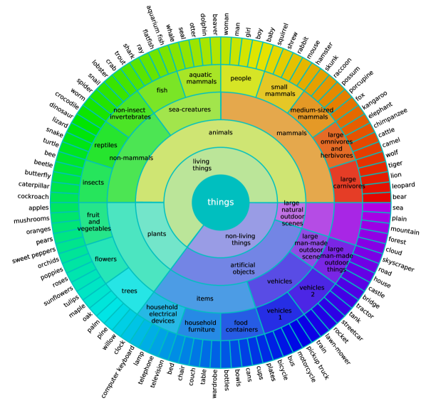
Figure 8: Class hierarchy for CIFAR100. The arcs at different radii represent the different classes of each level of the hierarchy. Unlabelled arcs share the same name as their parent class.

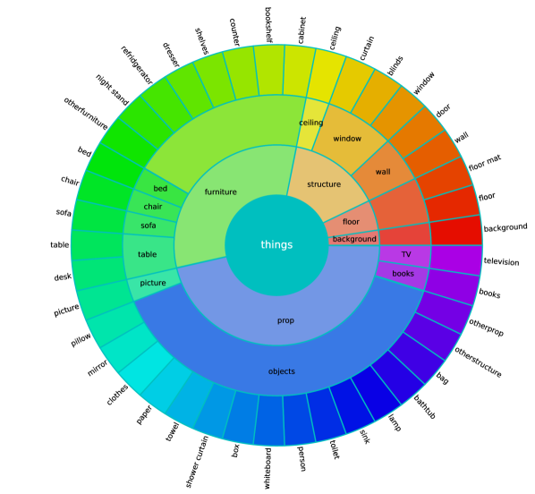
Figure 9: Class hierarchy for NYUv2

Figure 10: Class hierarchy for S2-Agri

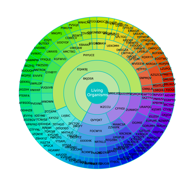
Figure 11: Class hierarchy for iNat-19, only the first $6$ levels of the hierarchy are represented. At the time of writing, only the classes’ obfuscated names were publicly available

Bibliography

- Naveed Akhtar and Ajmal Mian. Threat of adversarial attacks on deep learning in computer vision: A survey. IEEE Access, 2018.
- Shahanaz Ayub and JP Saini. ECG classification and abnormality detection using cascade forward neural network. International Journal of Engineering, Science and Technology, 2011.
- Luca Bertinetto, Romain Mueller, Konstantinos Tertikas, Sina Samangooei, and Nicholas A Lord. Making better mistakes: Leveraging class hierarchies with deep networks. In CVPR, 2020.
- Jean Bourgain. On Lipschitz embedding of finite metric spaces in Hilbert space. Israel Journal of Mathematics, 1985.
- Gerhard Brankatschk and Matthias Finkbeiner. Modeling crop rotation in agricultural lcas—challenges and potential solutions. Agricultural Systems, 2015.
- Donald G Bullock. Crop rotation. Critical reviews in plant sciences, 1992.
- Samuel Rota Bulo, Gerhard Neuhold, and Peter Kontschieder. Loss max-pooling for semantic image segmentation. In CVPR, 2017.
- Chris Burges, Tal Shaked, Erin Renshaw, Ari Lazier, Matt Deeds, Nicole Hamilton, and Greg Hullender. Learning to rank using gradient descent. In ICML, 2005.
- Chaofan Chen, Oscar Li, Daniel Tao, Alina Barnett, Cynthia Rudin, and Jonathan K Su. This looks like that: deep learning for interpretable image recognition. In NeurIPS, 2019.
- Christopher De Sa, Albert Gu, Christopher Ré, and Frederic Sala. Representation tradeoffs for hyperbolic embeddings. In Proceedings of Machine Learning Research, 2018.
- Jia Deng, Alexander C Berg, Kai Li, and Li Fei-Fei. What does classifying more than 10,000 image categories tell us? In ECCV, 2010.
- Nanqing Dong and Eric Xing. Few-shot semantic segmentation with prototype learning. In BMVC, 2018.
- Steven Fortune. Voronoi diagrams and Delaunay triangulations. In Computing in Euclidean Geometry. World Scientific, 1992.
- Andrew Gelman, John B Carlin, Hal S Stern, David B Dunson, Aki Vehtari, and Donald B Rubin. Bayesian data analysis. CRC press, 2013.
- Wyn Grant. The common agricultural policy. Macmillan International Higher Education, 1997.
- Samantha Guerriero, Barbara Caputo, and Thomas Mensink. DeepNCM: deep nearest class mean classifiers. In ICLR, Worskhop, 2018.
- Saurabh Gupta, Pablo Arbelaez, and Jitendra Malik. Perceptual organization and recognition of indoor scenes from RGB-D images. In CVPR, 2013.
- A Handa, V Patraucean, V Badrinarayanan, S Stent, and R Cipolla. Uunderstanding real world indoor scenes with synthetic data. In CVPR, 2016.
- Caner Hazirbas, Lingni Ma, Csaba Domokos, and Daniel Cremers. Fusenet: Incorporating depth into semantic segmentation via fusion-based CNN architecture. In ACCV, 2016.
- Kaiming He, Xiangyu Zhang, Shaoqing Ren, and Jian Sun. Deep residual learning for image recognition. In CVPR, 2016.
- Le Hou, Chen-Ping Yu, and Dimitris Samaras. Squared earth mover’s distance-based loss for training deep neural networks. In NeurIPS Workshop, 2016.
- Piotr Indyk, Jiří Matoušek, and Anastasios Sidiropoulos. Low-distortion embeddings of finite metric spaces. In Handbook of discrete and computational geometry. Chapman and Hall/CRC, 2017.
- Saumya Jetley, Bernardino Romera-Paredes, Sadeep Jayasumana, and Philip Torr. Prototypical priors: From improving classification to zero-shot learning. In BMVC, 2015.
- Shyamgopal Karthik, Ameya Prabhu, Puneet K Dokania, and Vineet Gandhi. No cost likelihood manipulation at test time for making better mistakes in deep networks. ICLR, 2021.
- Valentin Khrulkov, Leyla Mirvakhabova, Evgeniya Ustinova, Ivan Oseledets, and Victor Lempitsky. Hyperbolic image embeddings. In CVPR, 2020.
- Teuvo Kohonen. Learning vector quantization. In Self-organizing maps. Springer, 1995.
- Aris Kosmopoulos, Ioannis Partalas, Eric Gaussier, Georgios Paliouras, and Ion Androutsopoulos. Evaluation measures for hierarchical classification: a unified view and novel approaches. Data Mining and Knowledge Discovery, 2015.
- Alex Krizhevsky, Geoffrey Hinton, et al. Learning multiple layers of features from tiny images. Technical report, University of Toronto, 2009.
- Tsung-Yi Lin, Priya Goyal, Ross Girshick, Kaiming He, and Piotr Dollár. Focal loss for dense object detection. In ICCV, 2017.
- Shaoteng Liu, Jingjing Chen, Liangming Pan, Chong-Wah Ngo, Tat-Seng Chua, and Yu-Gang Jiang. Hyperbolic visual embedding learning for zero-shot recognition. In CVPR, 2020.
- Teng Long, Pascal Mettes, Heng Tao Shen, and Cees GM Snoek. Searching for actions on the hyperbole. In CVPR, 2020.
- Pascal Mettes, Elise van der Pol, and Cees Snoek. Hyperspherical prototype networks. In NeurIPS, 2019.
- Tomas Mikolov, Kai Chen, Greg Corrado, and Jeffrey Dean. Efficient estimation of word representations in vector space. In ICLR Workshop, 2013.
- George A Miller, Richard Beckwith, Christiane Fellbaum, Derek Gross, and Katherine J Miller. Introduction to wordnet: An on-line lexical database. International Journal of Lexicography, 1990.
- Pushmeet Kohli Nathan Silberman, Derek Hoiem and Rob Fergus. Indoor segmentation and support inference from RGBD images. In ECCV, 2012.
- Maximillian Nickel and Douwe Kiela. Poincaré embeddings for learning hierarchical representations. In NeurIPS, 2017.
- Joseph Redmon and Ali Farhadi. YOLO9000: better, faster, stronger. In CVPR, 2017.
- Deboleena Roy, Priyadarshini Panda, and Kaushik Roy. Tree-CNN: a hierarchical deep convolutional neural network for incremental learning. Neural Networks, 2020.
- Olga Russakovsky, Jia Deng, Hao Su, Jonathan Krause, Sanjeev Satheesh, Sean Ma, Zhiheng Huang, Andrej Karpathy, Aditya Khosla, Michael Bernstein, et al. Imagenet large scale visual recognition challenge. International Journal of Computer Vision, 2015.
- Vivien Sainte Fare Garnot, Loic Landrieu, Sebastien Giordano, and Nesrine Chehata. Satellite image time series classification with pixel-set encoders and temporal self-attention. In CVPR, 2020.
- Ruslan Salakhutdinov, Joshua B Tenenbaum, and Antonio Torralba. Learning with hierarchical-deep models. IEEE Transactions on Pattern Analysis and Machine Intelligence, 2012.
- Atsushi Sato and Keiji Yamada. Generalized learning vector quantization. NeurIPS, 1995.
- Abhinav Shrivastava, Abhinav Gupta, and Ross Girshick. Training region-based object detectors with online hard example mining. In CVPR, 2016.
- Carlos N Silla and Alex A Freitas. A survey of hierarchical classification across different application domains. Data Mining and Knowledge Discovery, 2011.
- Jake Snell, Kevin Swersky, and Richard Zemel. Prototypical networks for few-shot learning. In NeurIPS, 2017.
- Nitish Srivastava and Russ R Salakhutdinov. Discriminative transfer learning with tree-based priors. In NeurIPS, 2013.
- Kah-Kay Sung. Learning and example selection for object and pattern detection. MIT A.I., 1996.
- Robert Tibshirani, Trevor Hastie, Balasubramanian Narasimhan, and Gilbert Chu. Diagnosis of multiple cancer types by shrunken centroids of gene expression. Proceedings of the National Academy of Sciences, 2002.
- Grant Van Horn, Oisin Mac Aodha, Yang Song, Yin Cui, Chen Sun, Alex Shepard, Hartwig Adam, Pietro Perona, and Serge Belongie. The iNaturalist species classification and detection dataset. In CVPR, 2018.
- Zhicheng Yan, Hao Zhang, Robinson Piramuthu, Vignesh Jagadeesh, Dennis DeCoste, Wei Di, and Yizhou Yu. HD-CNN: hierarchical deep convolutional neural networks for large scale visual recognition. In ICCV, 2015.
- Hong-Ming Yang, Xu-Yao Zhang, Fei Yin, and Cheng-Lin Liu. Robust classification with convolutional prototype learning. In CVPR, 2018.