Deep Contextual Embeddings for Address Classification in E-commerce

Abstract.

E-commerce customers in developing nations like India tend to follow no fixed format while entering shipping addresses. Parsing such addresses is challenging because of a lack of inherent structure or hierarchy. It is imperative to understand the language of addresses, so that shipments can be routed without delays. In this paper, we propose a novel approach towards understanding customer addresses by deriving motivation from recent advances in Natural Language Processing (NLP). We also formulate different pre-processing steps for addresses using a combination of edit distance and phonetic algorithms. Then we approach the task of creating vector representations for addresses using Word2Vec with TF-IDF, Bi-LSTM and BERT based approaches. We compare these approaches with respect to sub-region classification task for North and South Indian cities. Through experiments, we demonstrate the effectiveness of generalized RoBERTa model, pre-trained over a large address corpus for language modelling task. Our proposed RoBERTa model achieves a classification accuracy of around 90% with minimal text preprocessing for sub-region classification task outperforming all other approaches. Once pre-trained, the RoBERTa model can be fine-tuned for various downstream tasks in supply chain like pincode suggestion and geo-coding. The model generalizes well for such tasks even with limited labelled data. To the best of our knowledge, this is the first of its kind research proposing a novel approach of understanding customer addresses in e-commerce domain by pre-training language models and fine-tuning them for different purposes.

1. Introduction

Machine processing of manually entered addresses poses a challenge in developing countries because of a lack of standardized format. Customers shopping online tend to enter shipping addresses with their own notion of correctness. This creates problems for e-commerce companies in routing shipments for last mile delivery. Consider the following examples of addresses entered by customers:

1. ‘XXX, AECS Layout, Geddalahalli, Sanjaynagar main Road Opp. Indian Oil petrol pump, Ramkrishna Layout, Bengaluru Karnataka 560037’
   

2. ‘XXX, B-Block, New Chandra CHS, Veera Desai Rd, Azad Nagar 2, Jeevan Nagar, Azad Nagar, Andheri West, Mumbai, Maharashtra 400102’
   

3. ‘Gopalpur Gali XXX, Near Hanuman Temple, Vijayapura, Karnataka 586104’
   

4. ‘Sector 23, House number XXX, Faridabad, Haryana 121004’
   

5. ‘H-XXX, Fortune Residency, Raj Nagar Extension Ghaziabad Uttar Pradesh 201003’

It is evident from above illustrations that addresses do not tend to follow any fixed pattern and consist of tokens with no standard spellings. Thus, applying Named Entity Recognition (NER) systems to Indian addresses for sub-region classification becomes a challenging problem. Devising such a system for Indian context requires a large labelled dataset to cover all patterns across the geography of a country and is a tedious task. At the same time, Geo-location information which otherwise makes the problem of sub-region classification trivial, is either not readily available or is expensive to obtain. In spite of all these challenges, e-commerce companies need to deliver shipments at customer doorstep in remote as well as densely populated areas. At this point, it becomes necessary to interpret and understand the language of noisy addresses at scale and route the shipments appropriately. Many a times, fraudsters tend to enter junk addresses and e-commerce players end up incurring unnecessary shipping and reverse logistic costs. Hence, it is important to flag incomplete addresses while not being too strict on the definition of completeness. In recent years, the focus of NLP research has been on pre-training language models over large datasets and fine-tuning them for specific tasks like text classification, machine translation, question answering etc. In this paper, we propose methods to pre-process addresses and learn their latent representations using different approaches. Starting from traditional Machine Learning method, we explore sequential network(Hochreiter and Schmidhuber, 1997) and Transformer(Vaswani et al., 2017) based model to generate address representations. We compare these different paradigms by demonstrating their performance over sub-region classification task. We also comment on the limitations of traditional Machine Learning approaches and advantages of sequential networks over them. Further, we talk about the novelty of Transformer based models over sequential networks in the context of addresses. The contribution of the paper is as follows:

1. Details the purpose and challenges of parsing noisy addresses

2. Introduces multi-stage address preprocessing techniques

3. Proposes three approaches to learn address representations and their comparison with respect to sub-region classification task

4. Describes advantages of BERT based model as compared to traditional methods and sequential networks in the context of Indian addresses

The rest of the paper is organized as follows: In Section 2, we review previous works that deal with addresses in e-commerce. Next we present insights into the problem that occur in natural language addresses in Section 3 and propose pre-processing steps for addresses in Section 4. In Section 5, we present different approaches to learn latent address representations with sub-region classification task. In Section 6, we outline the experimental setup and present the results and visualizations of our experiments in Section 7. We present error analysis in Section 8 where we try to explain the reasons behind misclassified instances. Finally, we conclude the paper and discuss future work in Section 9.

2. Related Work

Purves and Jones (2011) provide a detailed account of seven major issues in Geographical Information Retrieval such as detecting and disambiguation of toponyms, geographical relevant ranking and user interfaces. Among them, the challenges of vague geographic terminology and spatial and text indexing are present in the current problem. Some such frequently occurring spatial language terms in the addresses include ‘near’, ‘behind’ and ‘above’. Ozdamar and Demir (2012) propose hierarchical cluster and route procedure to coordinate vehicles for large scale post-disaster distribution and evaluation. Gevaers et al. (2011) provide a description of the last mile problem in logistics and the challenges uniquely faced by last mile unlike any other component in supply chain logistics. Babu et al. (2015) show methods to classify textual address into geographical sub-regions for shipment delivery using Machine Learning. Their work mainly involves address pre-processing, clustering and classification using ensemble of classifiers to classify the addresses into sub-regions. Seng (2019) work on Malaysian addresses and classify them into different property types like condominium, apartments, residential homes ( bungalow, terrace houses, etc.) and business premises like shops, factories, hospitals, and so on. They use Machine Learning based models and also propose LSTM based models for classifying addresses into property types. Kakkar and Babu (2018) discuss the challenges with address data in Indian context and propose methods for efficient large scale address clustering using conventional as well as deep learning techniques. They experiment with different variants of Leader clustering using edit distance, word embedding etc. For detecting fraud addresses over e-commerce platforms and reduce operational cost, Babu and Kakkar (2017) propose different Machine Learning methodologies to classify addresses as ‘normal’ or ‘monkey-typed’(fraud). In order to represent addresses of populated places, Kejriwal and Szekely (2017) train a neural embedding algorithm based on skip-gram(Mikolov et al., 2013) architecture to represent each populated place into a 100-dimensional vector space. For Neural Machine Translation (NMT), Vaswani et al. (2017) propose Transformer model which is based solely on attention mechanisms, moving away from recurrence and convolutions. The transformer model significantly reduces training time due to its positional embeddings based parallel input architecture. Devlin et al. (2018) propose BERT architecture, which stands for Bidirectional Encoder Representations from Transformers. They demonstrate that BERT obtains state-of-the-art performance on several NLP tasks like question answering, classification etc. Liu et al. (2019) propose RoBERTa which is a robust and optimized version of pre-training a BERT based model and achieve new state-of-the-art results on GLUE(Wang et al., 2018), RACE(Lai et al., 2017) and SQuAD(Rajpurkar et al., 2016) datasets.
To the best of our knowledge, there is no prior work that treats the problem of understanding addresses from a language modelling perspective. We experiment with different paradigms and demonstrate the efficacy of a BERT based model, pre-trained over a large address corpus for the downstream task of sub-region classification.

3. Problem Insights

Sorting shipments based on addresses forms an integral part of e-commerce operations. When a customer places an order online, items corresponding to the order are packed at a warehouse and dispatched for delivery. During the course of its journey from warehouse to the customer doorstep, the shipment undergoes multiple levels of sortation. The first level of sort is very broad and typically happens at the warehouse itself where multiple shipments are clubbed together in a ‘master bag’ on a state level and dispatched to different hubs. At the hub, another sort takes place on a city level and shipments are dispatched to the respective cities. As customers usually provide their state and city information accurately, sorting at the warehouse and the hub becomes a trivial process. Once shipments reach a city, they are sub-divided into different zones. Each zone is further divided into multiple sub-regions. The sub-regions can take highly irregular shapes depending on density of customers, road network and ease of delivery. Figure 1 shows different sub-regions for last mile delivery of shipments. These sub-regions constitute the class definitions for our problem. The challenge in last mile delivery emerges when customers are unsure of their locality names and pincodes. The ambiguity arises because of the unstructured nature of localities and streets in developing nations. Coupled with this, area names originating from colloquial languages make it difficult for users to enter their shipping addresses in English, resulting in multiple spell variants of localities, sometimes in hundreds. Solutions for parsing addresses (Craig et al., 2019) have been proposed in the past but they seldom work for cities in developing nations like India, Nepal and Bangladesh where there is no standard way of writing an address. The notion of sufficiency of information for a successful delivery is subjective and depends on multiple factors like the address text, familiarity of locality for the delivery agent, availability of customers’ phone numbers in case of confusion and so on. In planned cities, areas are generally divided into blocks (sectors) and thus mentioning the house number and name of the sector might be sufficient for a delivery agent. But in unplanned cities, where a huge majority of the population resides, locality definition become very subjective. Deciphering pincodes is also a cumbersome task, especially at the boundaries. As a result, customers end up entering noisy addresses for the last mile. For the purpose of the problem described in this paper, we ignore phone numbers of customers as a source of information and work with text addresses only. For solving the challenges of last mile delivery, we propose address preprocessing methods. Subsequently, we describe ways to use state-of-the-art NLP approaches to obtain address representations which can be used for various downstream tasks.

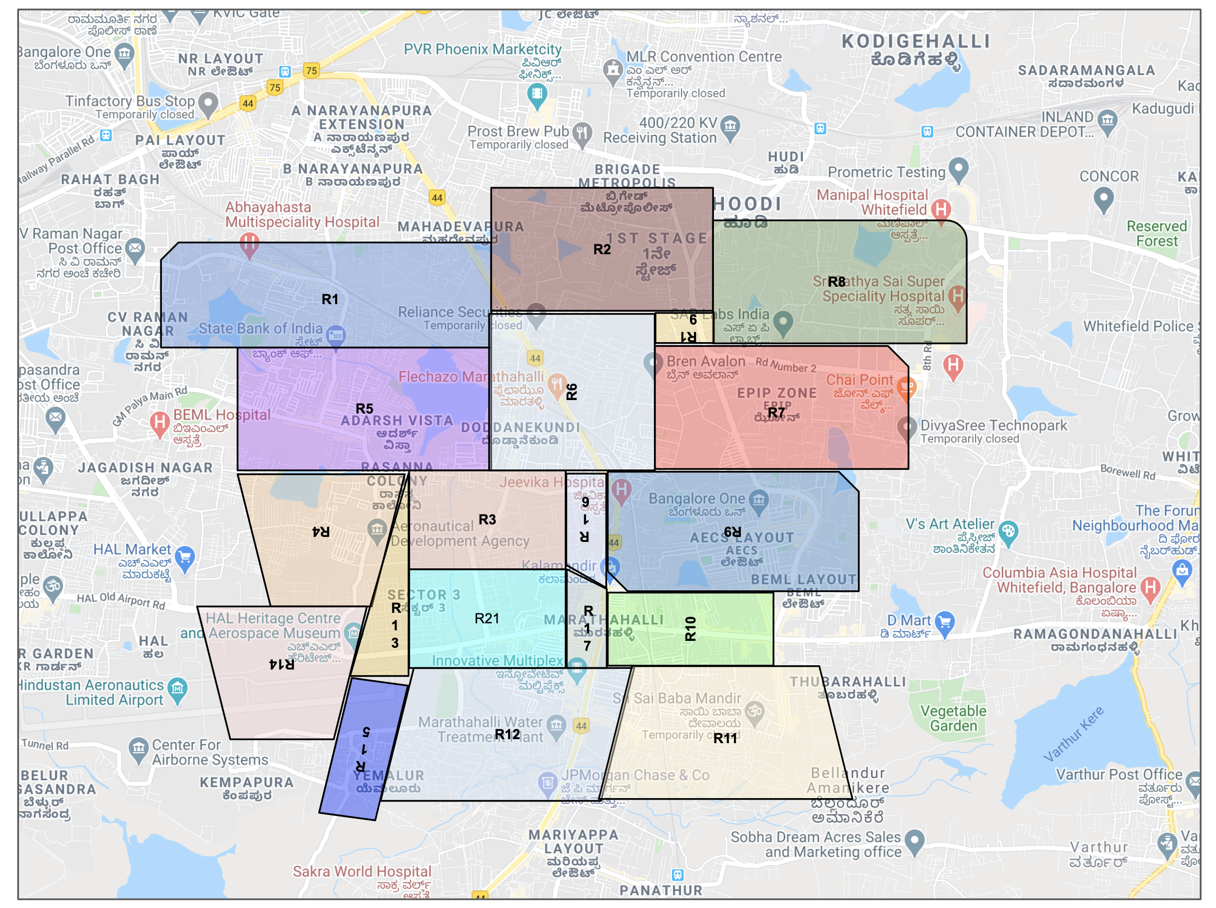
Figure 1. Sample map depicting sub-regions for last mile delivery.

4. Address Pre-processing

We propose different pre-processing steps for addresses. Our analysis indicates that customers generally tend to make mistakes while entering names of localities and buildings broadly due to two reasons:

1. Input errors while typing, arising mainly due to closeness of characters in the keyboard

2. Uncertainty regarding ‘correct’ spellings of locality/street names

The notion of ‘correct spelling’ is itself subjective and we consider the correct spelling to be the one entered most frequently by customers. In our work, we bucket the errors into four categories in Table 1. The second column shows address tokens and their correct form.

Error Type	Example
Missing white space between correctly spelled tokens	meenakshiclassic $\rightarrow$ meenakshi classic
Redundant whitespace between correctly spelled tokens	lay out $\rightarrow$ layout
Misspelled individual tokens	appartments $\rightarrow$ apartments
Misspelled compound tokens with no whitespace	sectarnoida $\rightarrow$ sector noida

Table 1. Types of errors encountered in Indian Addresses.

For traditional ML approaches, directly using raw addresses without spell correction leads to a larger vocabulary size bringing in problems of high dimensionality and over-fitting. Standard English language Stemmers and Lemmatizers do not yield satisfactory results for vocabulary reduction because of code-mixing (Bokamba, 1988) issues in addresses. Hence we need to devise custom methods for reducing the vocabulary size by correcting for spell variations. We illustrate different methods for solving each of the errors mentioned in Table 1. Figure 2 shows the overall steps involved in address preprocessing.

4.1. Basic Cleaning

We begin by performing a basic pre-processing of addresses which includes removal of special characters and lower-casing of tokens. We remove all the numbers which are of length greater than six as some customers enter phone numbers and pincodes in the address field. Address tokens are generated by splitting on whitespace character. We append pincodes to addresses after applying all the pre-processing steps.

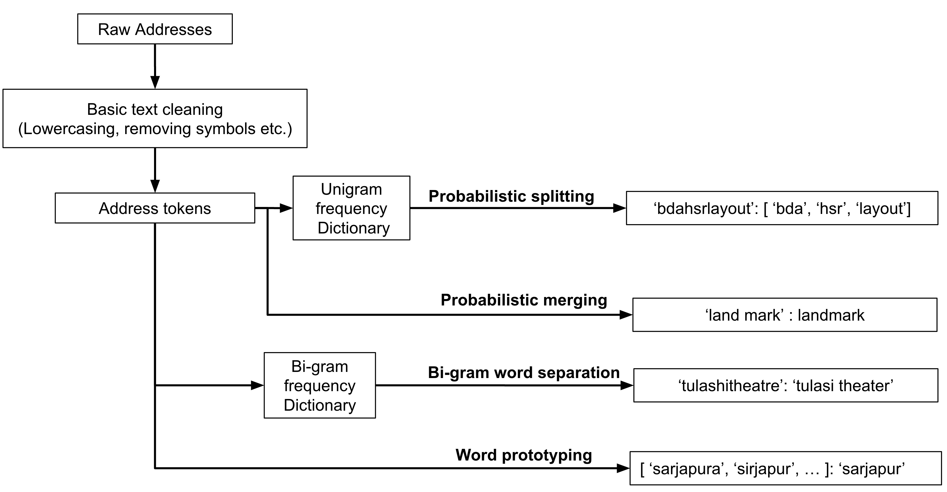
Figure 2. Flow-Diagram depicting address pre-processing methods.

4.2. Probabilistic splitting

The motivation for this technique comes from Babu et al. (2015). In this step, we perform token separation using count frequencies in a large corpus of customer addresses. The first step is to construct a term-frequency dictionary for the corpus. Following this, we iterate through the corpus and split each token at different positions to check if the resulting count of individual tokens after splitting is greater than the compound token. In such cases, we store the instance in a separate dictionary which we can use for preprocessing addresses at runtime. Consider the compound token ‘hsrlayout’, the method iteratively splits this token at different positions and finally results in ‘hsr’ and ‘layout’ as the joint probability of these tokens exceeds the probability of ‘hsrlayout’.

4.3. Spell correction

In order to determine the right spell variant and correct for variations, we cluster tokens in our corpus using leader clustering (Ling, 1981). This choice emanates from the fact that leader clustering is easy to implement and does not require specifying the number of clusters in advance and has a complexity of $O(n)$. We recursively cluster the tokens in our corpus using Levenshtein distance (Levenshtein, 1966) coupled with Metaphone algorithm (Philips, 1990). We use a combination of these algorithms as standalone use of either of them has some drawbacks. While using only edit distance based clustering, we observe that many localities which differ by a single character but are phonetically different tend to get clustered together. For example, in a city like Bangalore we find two distinct localities with names ‘Bommasandra’ and ‘Dommasandra’ which differ by a single character. While using only the edit distance condition, all instances of the former will be tagged with the latter or vice-versa depending on which locality occurs more frequently in the corpus. This will result in erroneous outputs for downstream tasks. In the above instance, we observe that the two locality names are phonetically different and a phonetic algorithm will output different hash values and thus help in assigning them to separate clusters. When using only phonetic based approach, we find that some distinct locality names are clustered together. For example, two localities by the name ‘Mathkur’ and ‘Mathikere’ have the same hash value according to Metaphone algorithm. In this case, even though the two locality names have similar phonetic hash values, by using an edit distance threshold we can ensure that the two are not clustered together. This inspires our choice of a combination of edit distance and phonetic algorithms for clustering spell variants. The most frequently occurring instance within each cluster is selected as the ‘leader’. In order to perform spell correction, we replace each spell variant with its corresponding leader. The key principle behind spell correction for addresses is summarized below. Consider two tokens $\boldsymbol{T_{a}}$ and $\boldsymbol{T_{b}}$. We say $\boldsymbol{T_{a}}$ is a spell variant of $\boldsymbol{T_{b}}$ if:

$Count(\boldsymbol{T_{a}})<Count(\boldsymbol{T_{b}})$

&

$LevenshteinDistance(\boldsymbol{T_{a}},\boldsymbol{T_{b}})<threshold$

&

$Metaphone(\boldsymbol{T_{a}})==Metaphone(\boldsymbol{T_{b}})$

For experiments, we set $threshold$ value equal to 3 and only consider tokens of length greater than 6 as candidates for spell correction.

4.4. Bigram separation

Probabilistic splitting of compound tokens described in Section 4.2 can work only when individual tokens after splitting have a support larger than the compound token. If there is a missing white space coupled with a spelling error, probabilistic word splitting will not be able to separate the tokens. This is because the incorrect spell variant will not have enough support in the corpus. For this reason, we propose bi-gram word separation using leader clustering. At first, we construct a dictionary of all bi-grams occurring in our corpus as keys and number of occurrences as values. These bigrams are considered as single tokens and we iterate through the corpus and cluster the address tokens using leader clustering algorithm with edit distance threshold and phonetic matching condition. For example, ‘bangalore karnataka’ is a bigram which occurs frequently in the corpus. Against this ‘leader’, different erroneous instances get assigned like ‘bangalorkarnataka’, ‘bangalorekarnatak’ etc. These instances cannot be split using ‘Probabilistic splitting’ described in Section 4.2 since the tokens ‘bangalor’ and ‘karnatak’ do not have significant support in the corpus. We store the bigrams and their error variants in a dictionary and use it for address pre-processing in the downstream tasks.

4.5. Probabilistic merging

Customers often enter unnecessary whitespaces while typing addresses. For correcting such instances, we propose probabilistic merging similar to the method described in Section 4.2. Instead of splitting the tokens, we merge adjacent tokens in the corpus if the compound token has a higher probability of occurrence compared to the individual tokens. For example, the tokens ‘lay’ and ‘out’ will have a significantly lesser count than the compound token ‘layout’ and thus all such instances where the token ‘lay’ occurs followed by ‘out’ will be replaced with ‘layout’.

5. Approaches

We demonstrate the use of three different paradigms: Traditional Machine Learning, Bi-LSTMs and BERT based model for generating latent address representations and use them for sub-region classification task. Through our experiments, we observe the effectiveness of generalized RoBERTa model, pre-trained over a large address corpus for language modelling task. We also comment on the limitations of traditional machine learning approaches and advantages of sequential networks. Further, we talk about the novelty of RoBERTa model over sequential networks in the context of addresses.

5.1. Word2Vec with TF-IDF

As a baseline approach we use the techniques described in Section 4 to pre-process addresses and use them to train a Word2Vec model (Mikolov et al., 2013) for obtaining vector representation of tokens in an address. Further we compute Term Frequency - Inverse Document Frequency (TF-IDF)(Salton and McGill, 1986) values for each token within an address and use them as weights for averaging the word vectors to obtain representation for an address. Weighting the tokens within an address is necessary since not all tokens in an address are equally ‘important’ from a classification standpoint. Generally, we find that locality/landmark is the most important token, even for humans to identify the right sub-region. But in many instances, it is not very straight forward to be able to point at the appropriate information necessary for classification. Thus, in order to make the model automatically identify the most important tokens in an address, we use the TF-IDF concept. TF-IDF is a statistical measure of how important a word is to a document in a collection or corpus. Term Frequency (TF) denotes the frequency of a term within a document and Document Frequency (DF) is a measure of the number of documents in which a particular term occurs. Mathematically, it can be defined as follows:

(1) $$\textbf{TF}(t,d)=f_{t,d}$$

(2) $$\textbf{IDF}(t,D)=log\frac{N}{|\{d\in D:t\in d\}|}$$

In our case, an address is a document $\boldsymbol{d}$, each token in the address is $\boldsymbol{t}$, the collection of addresses is the corpus $\boldsymbol{D}$ and total number of addresses is $\boldsymbol{N}$. The TF-IDF statistic by definition assigns a lower weight to very frequent tokens. For our case, city names are typically mentioned in all the addresses and thus are not of much value. Contrary to city names, customers sometime enter information like detailed directions to reach their door step which form rare tokens in our corpus. In such cases, TF-IDF assigns the maximum weight of $log(N)$ and we remove such tokens while constructing address representations. We use these embeddings as features for training a multi-class classifier to classify addresses into sub-regions. A drawback of this approach is that, by averaging word vectors we end up losing the sequential information. For example, the addresses ‘House No. X, Sector Y, Faridabad’ and ‘House No. Y, Sector X, Faridabad’ end up producing the same address vectors and induce error in classification. In spite of this, it forms a strong baseline to assess the efficacy of more advanced approaches.

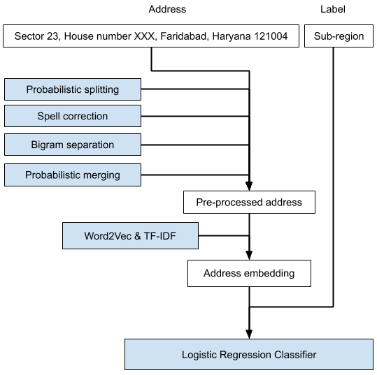
Figure 3. Logistic regression classifier with TF-IDF weighted Word2Vec vectors as features.

5.2. Bi-LSTM

Averaging word vectors leads to loss of sequential information, hence we move on to a Bi-LSTM(Hochreiter and Schmidhuber, 1997) based approach. While LSTMs are known to preserve the sequence information, Bi-directional LSTMs have an added advantage since they also capture both the left and right context in case of text classification. Given an input address of length T with words $w_{t}$, where $t\in[1,T]$. We convert each word $w_{t}$ to its vector representation $x_{t}$ using the embedding matrix $E$. We then use a Bi-directional LSTM to get annotations of words by summarizing information from both directions. Bidirectional LSTMs consist of a forward LSTM $\overrightarrow{f}$, which reads the address from $w_{1}$ to $w_{T}$ and a backward LSTM $\overleftarrow{f}$, which reads the address from $w_{T}$ to $w_{1}$:

(3) $$x_{t}=E^{T}w_{t},t\in[1,T]$$

(4) $$\overrightarrow{h_{t}}=\overrightarrow{LSTM}(x_{t}),t\in[1,T]$$

(5) $$\overleftarrow{h_{t}}=\overleftarrow{LSTM}(x_{t}),t\in[T,1]$$

We obtain representation for a given address token $w_{t}$ by concatenating the forward hidden state $\overrightarrow{h_{t}}$ and backward hidden state $\overleftarrow{h_{t}}$, i.e., $h_{t}=[\overrightarrow{h_{t}},\overleftarrow{h_{t}}]$, which summarizes the information of the entire address centered around $w_{t}$. The concatenation of final hidden state outputs of the forward and backward LSTMs is denoted by $h_{T}=[\overrightarrow{h_{T}},\overleftarrow{h_{T}}]$. This forms the address embedding which is then passed to a dense layer with softmax activation. We train this model by minimizing cross-entropy loss. Section 7 shows the improvement in performance due to the ability of LSTMs to better capture sequential information. The drawback with this approach is that training a Bi-LSTM model is relatively slow because of its sequential nature. Hence we experiment with Transformer based models which have parallelism in-built.

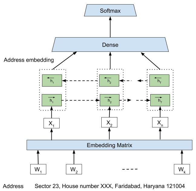
Figure 4. Bi-LSTM architecture for Address classification.

5.3. RoBERTa

In this section, we experiment with RoBERTa(Liu et al., 2019) which is a variant of BERT(Devlin et al., 2018), for pre-training over addresses and fine-tune it for sub-region classification task. The BERT model optimizes over two auxiliary pre-training tasks:

• Mask Language Model (MLM): Randomly masking 15% of the tokens in each sequence and predicting the missing words

• Next Sentence Prediction (NSP): Randomly sampling sentence pairs and predicting whether the latter sentence is the next sentence of the former

BERT based representations try to learn the context around a word and is able to better capture its meaning syntactically and semantically. For our context, NSP loss does not hold meaning since customer addresses on e-commerce platforms are logged independently. This motivates the choice of RoBERTa model since it uses only the MLM auxiliary task for pre-training over addresses. In experiments we use byte-level BPE (Sennrich et al., 2015) tokenization for encoding addresses. We use perplexity(Chen et al., 2018) score for evaluating the RoBERTa language model. It is defined as follows:

(6) $$P(Sentence)=P(w_{1}w_{2}....w_{N})^{\frac{-1}{N}}$$

where P(Sentence) denotes the probability of a test sentence and $w_{1}$, $w_{2}$,…., $w_{N}$ denotes words in the sentence. Generally, lower is the perplexity, better is the language model. After pre-training, the model would have learnt the syntactic and semantic aspects of tokens in shipping addresses. Figure 5 shows the overall approach used to pre-train RoBERTa model and fine-tune it for sub-region classification.

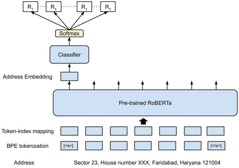
Figure 5. Pre-trained RoBERTa architecture for sub-region classification.

Dataset	Number of rows (addresses)	Number of classes (sub-regions)
Zone-1	98,868	42
Zone-2	93,991	20
Zone-3	106,421	86
Zone-4	218,434	176

Table 2. Dataset details for sub-region classification.

6. Experimental Setup

We experiment with four labelled datasets, two each from North and South Indian cities. The datasets are coded as Zone-1, Zone-2 from South India and Zone-3, Zone-4 from North India. Table 2 captures the details of all four datasets in terms of their size and number of classes. Each class represents a sub-region within a zone, which typically corresponds to a locality or multiple localities. The geographical area covered by a class (sub-region) varies with customer density. Thus, boundaries of these regions when drawn over a map can take extremely irregular shapes as depicted in Figure 1. All the addresses are unique and do not contain exact duplicates. For the purpose of address classification, we do not remove cases where multiple customers ordering from the same location have written their address differently. This happens in cases where customers order from their office location or when family members order from the same house through different accounts. We set aside 20% of rows randomly selected from each of the 4 labelled dataset as holdout test set. For all modelling approaches, we experiment with two variations of address pre-processing: Applying only the basic pre-processing step of Section 4.1 to addresses and applying all the steps mentioned in Section 4. In Table 3, we report the classification results of all the proposed approaches. For Word2Vec with TF-IDF based approach, we train a Word2Vec model over address dataset using the Gensim(Řehůřek and Sojka, 2010) library with vectors of dimension $100$, window size of $5$ and use it in our baseline approach mentioned in 5.1. We train a logistic classifier with $L2$ regularization using scikit-learn(Pedregosa et al., 2011) for $5000$ iterations

Modelling Approaches	Full Pre-Processing	Zone-1	Zone-2	Zone-3	Zone-4
Averaging Word2Vec tokens	No	0.77	0.79	0.76	0.80
Word2Vec + TF-IDF	No	0.81	0.82	0.80	0.83
Word2Vec + TF-IDF	Yes	0.85	0.84	0.82	0.85
Bi-LSTM w/o pre-trained word embeddings	No	0.88	0.87	0.83	0.88
Bi-LSTM with pre-trained word embeddings	Yes	0.89	0.88	0.84	0.90
Pre-trained RoBERTa from hugging face	No	0.89	0.90	0.85	0.91
Custom Pre-trained RoBERTa	No	0.88	0.91	0.84	0.92
Custom Pre-trained RoBERTa	Yes	0.90	0.88	0.85	0.91

Table 3. Accuracy numbers for different approaches for sub-region classification task.

Dataset	Number of rows (addresses)	Perplexity
Combined Dataset with basic pre-processing	106,421	4.509
Combined Dataset with full pre-processing	218,434	5.07

Table 4. Perplexity scores for RoBERTa pre-trained over Indian addresses for language modelling task.

in order to minimize cross-entropy loss. For Bi-LSTM based approach, we experiment with two scenarios:

1. Training Bi-LSTM network by randomly initializing Embedding Matrix

2. Training Bi-LSTM network by initializing Embedding Matrix with pre-trained word vectors obtained in Section 5.1

We pre-pad the tokens to obtain a uniform sequence length of $max\_length=60$ for all the addresses. We use softmax activation in the dense layer with Adam(Kingma and Ba, 2014) optimizer and Cross Entropy loss. The training and testing is performed individually on each of the four datasets and the number of epochs is chosen using cross-validation. For RoBERTa model, we pre-train the ‘DistilRoBERTa-base’ from HuggingFace (Wolf et al., 2019). The model is distilled from ‘roberta-base’ checkpoint and has 6-layer, 768-hidden, 12-attention heads, 82M parameters. DistilRoBERTa-base is faster while not compromising much on performance (Sanh et al., 2019). Pre-training is done on NVIDIA TESLA P100 GPU with a vocabulary size of 30,000 on a combined dataset of North and South Indian addresses referred as combined dataset. We experiment with two variations of address pre-processing for pre-training the model:

• Only basic pre-processing as described in Section 4.1

• Full pre-preprocessing using all the steps mentioned in Section 4

Pre-training of the model is done with the above pre-processing variations and the results are present in Table 4. The model is trained to optimize the Masked Language Modelling objective as mentioned in 5.3 for 4 epochs with a cumulative training time of 12 hours and a batch size of 64. The pre-training is done using Pytorch (Paszke et al., 2019) framework. For sub-region classification task, we fine tune the pre-trained RoBERTa model using ‘RobertaForSequenceClassification’(Wolf et al., 2019) and initialize it with our pre-trained RoBERTa model. Fine-tuning ‘RobertaForSequenceClassification’ optimizes for cross-entropy loss using AdamW (Kingma and Ba, 2014)(Loshchilov and Hutter, 2017) optimizer.

7. Results & Visualization

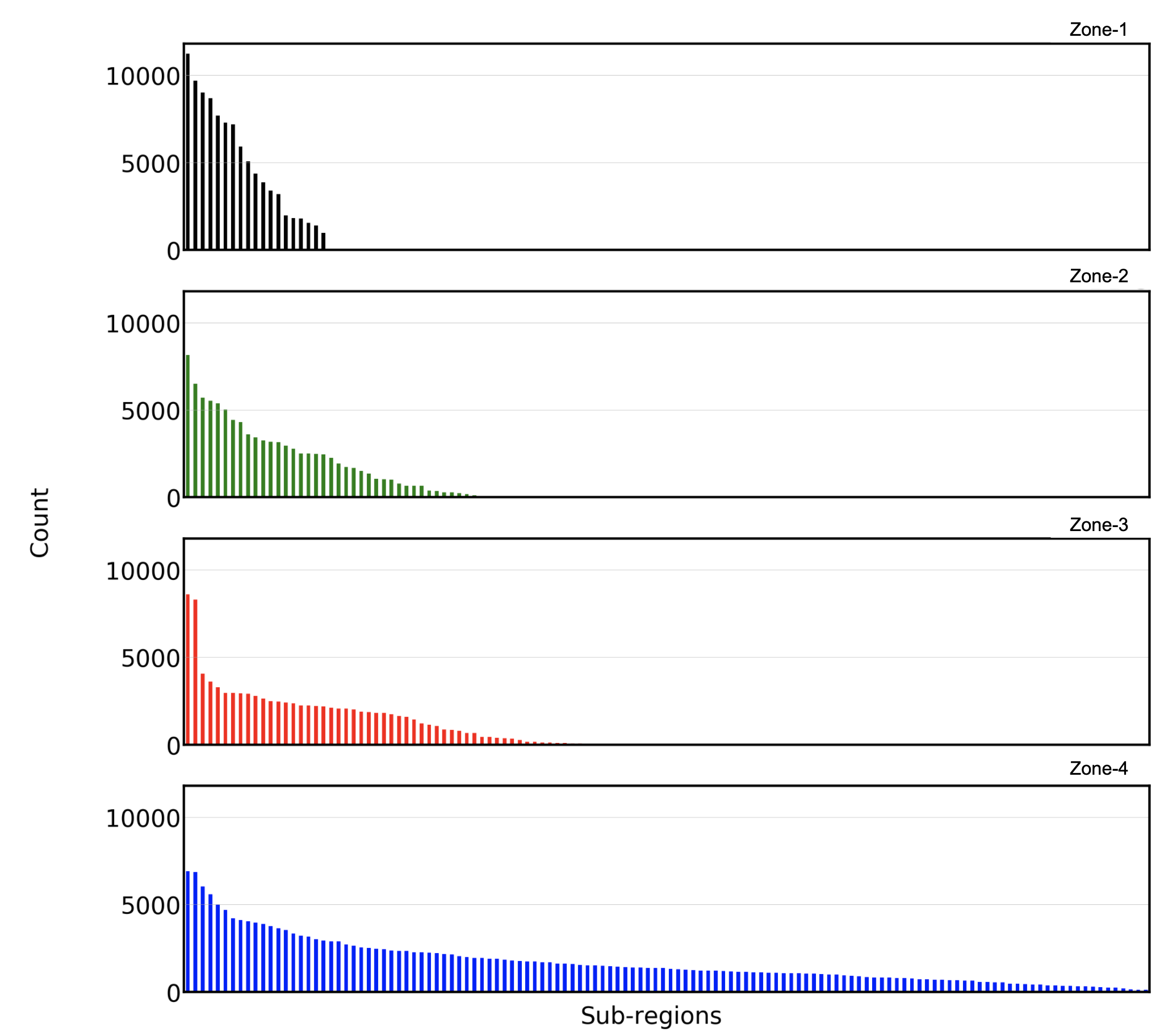
Figure 6. Class distribution of addresses for datasets mentioned in Table 2.

Table 2 lists the details of the datasets for the sub-region classification task. We use these datasets for evaluating each of the three different approaches mentioned in Section 5. Zone-1 and Zone-2 belong to South Indian Cities and Zone-3 and Zone-4 belong to North Indian cities. One can observe that the number of addresses in Zone-1 and Zone-2 are less as compared to Zone-3 and Zone-4. The number of sub-region/classes in Zone-3 and Zone-4 are 86 and 176 respectively, which are high compared to Zone-1/Zone-2. These differences occur due the fact that different zones cater to geographical areas with different population densities. Figure 6 shows the class distribution for the four datasets. We observe a skewed distribution since some sub-regions receive more shipments even though they are geographically small in size like office locations and large apartment complexes. Table 4 shows the combined dataset which we use for pre-training RoBERTa. We obtain a perplexity score of 4.51 for RoBERTa trained over combined dataset with basic pre-processing and with full pre-processing we observe it to be 5.07. The relatively lower perplexity scores are expected since the maximum length of addresses (sentences) after tokenization is 60 which is very less compared to the sequence lengths observed in NLP benchmark datasets like (Wang et al., 2018). Table 3 shows the accuracy values of different approaches for sub-region classification task performed on each of the four holdout test sets. A ‘Yes’ in the Full Pre-Processing column indicates that training is performed by applying full pre-processing and a ‘No’ indicates only basic pre-processing steps are applied. For Word2Vec based approaches, we experiment with three scenarios: $(1)$ Simple averaging of word vectors with basic pre-processing, $(2)$ Word2Vec with TF-IDF with basic pre-processing and $(3)$ Wor2Vec with TF-IDF with full pre-processing. Among these, the third setting achieves the best accuracy scores of 0.85, 0.84, 0.82 and 0.85 for Zone-1, Zone-2, Zone-3 and Zone-4 respectively indicating the efficacy of TF-IDF and address pre-processing techniques. Bi-LSTM based approach with pre-trained word embeddings is able to achieve best accuracy scores of 0.89, 0.88, 0.84 and 0.90 which shows that using pre-trained word vectors is advantageous compared to randomly initializing word vectors in the embedding matrix. For BERT based approaches, we compare RoBERTa model pre-trained using OpenWebTextCorpus(Gokaslan and Cohen, 2019) with the same pre-trained using combined dataset mentioned in Table 4. RoBERTa pre-trained on combined dataset of addresses with basic pre-processing is able to achieve accuracy scores of 0.88, 0.91, 0.84 and 0.92 respectively. Using combined dataset with full pre-processing for pre-training, the model achieves accuracy scores of 0.90, 0.88, 0.85 and 0.91. Hence, RoBERTa model pre-trained over a large address corpus for language modelling and fine-tuned for sub-region classification attains the highest accuracy scores compared to all other approaches indicating that custom pre-training over addresses is advantageous. Although the accuracy scores of Bi-LSTM and RoBERTa are comparable, there are some key differences between the two approaches. While Bi-LSTM networks are trained specifically for sub-region classification, the pre-trained RoBERTa model is only fine-tuned by training the last classification layer and hence can be used for multiple other downstream tasks using transfer learning. While we can also pre-train Bi-LSTM models as mentioned in Peters et al. (2018) and Howard and Ruder (2018), their performance over standard NLP benchmark datasets is significantly less as compared to BERT based models and motivates us to directly experiment with BERT based models for pre-training. BERT based models are more parallelizable owing to their non-sequential nature which is also a key factor in our choice of model for pre-training. Figure 7 shows the visualization of self attention weights for pre-trained Roberta model. We obtain these visualization using tool developed by Vig (2019). In the figure, edge density indicates the amount of weightage that is given to a particular token while optimizing for MLM loss in pre-training. We take a hypothetical example address: ‘room no 12 building no 257 srinivasa homes near kakatcafe hsr layout sector 3 560103’ for understanding the visualization. The figure at the top left shows the context in which number ‘12’ appears. From the figure it is visible that model has learned the representation in context of ‘room’ and ‘building’ which are associated with number ‘12’. The top right figure shows the association of number ‘257’ with context tokens: ‘building’, ‘no’ and ‘srinivasa’. Bottom left figure indicates the association of ‘layout’ with ‘hsr’ and the one at the bottom right indicates the association of ‘3’ with ‘sector’. We can observe from these visualizations that BERT based models incorporate the concept of self-attention by learning the embeddings for words based on the context in which they appear. From these visualizations one can find similarities in the way transformer models understand addresses and the way humans do, which is by associating different tokens to the context in which they appear. Figure 8 shows the violin plots of probability scores assigned to the predicted classes for different approaches. We plot results for the best models in all three approaches i.e Word2Vec with TF-IDF using full pre-processing, Bi-LSTM with pre-initialized word vectors and RoBERTa model pre-trained over address corpus with full address pre-processing. One can observe that the plots become more and more skewed towards the maximum as we move from left to right indicating a decrease in entropy of predicted probability scores. This is indicative of the higher confidence with which RoBERTa model is able to classify addresses as compared to other models.

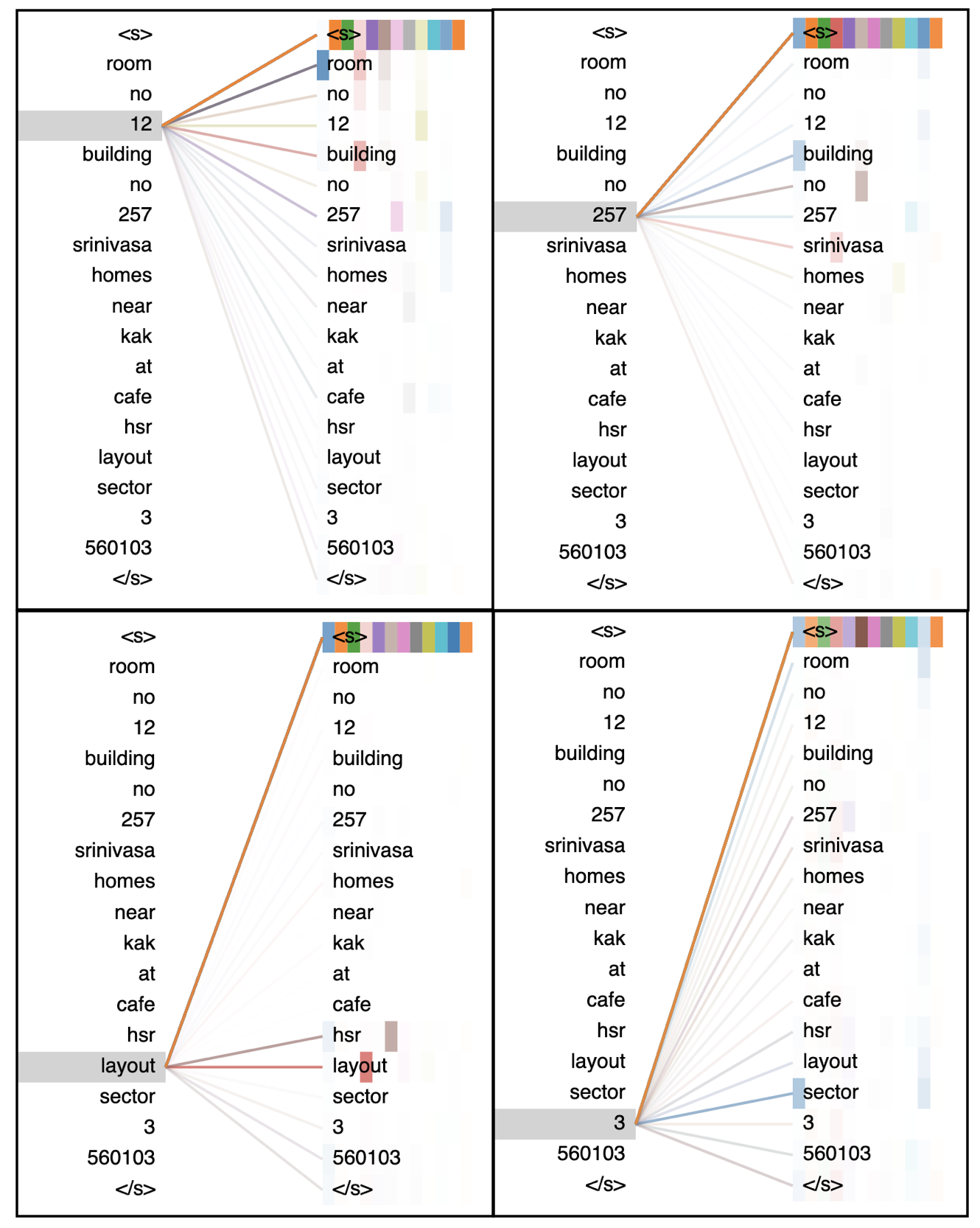
Figure 7. RoBERTa Multi-head Attention weights visualization.

8. Error Analysis

In this section, we present an analysis of the cases where the approaches presented in this paper fail to yield the expected result. The address pre-processing steps mentioned in Section 4 are heuristic methods and are prone to errors. Although these methods incorporate both edit distance threshold and phonetic matching conditions, they tend to fail in case of short-forms of tokens that customers use like ‘apt’ for ‘apartment’, ‘rd’ for ‘road’ etc. Also the pre-processing is dictionary based token substitution and hence it fails to correct tokens when new spell variants are encountered. For the approach described in Section 5.1, the model cannot account for sequential information in addresses. At the same time, Word2Vec approach is not able handle Out-Of-Vocabulary (OOV) tokens which poses a major hurdle with misspelled tokens in addresses. When locality names are misspelled, the tokens are simply ignored while computing the address embedding resulting in misclassification. For Bi-LSTM based approach mentioned in Section 5.2, the number of training parameters depend on the size of the tokenizer vocabulary. The tokenizer treats all OOV tokens as ‘UNK’ (Unknown) and thus, even in this approach the OOV problem persists. Roberta model described in Section 5.3 is able to handle spell variations as well as out of vocabulary words using BPE encoding. In this scenario, we can set a desired vocabulary size and the OOV tokens are split into sub-tokens. When we analyze the misclassified instances of our

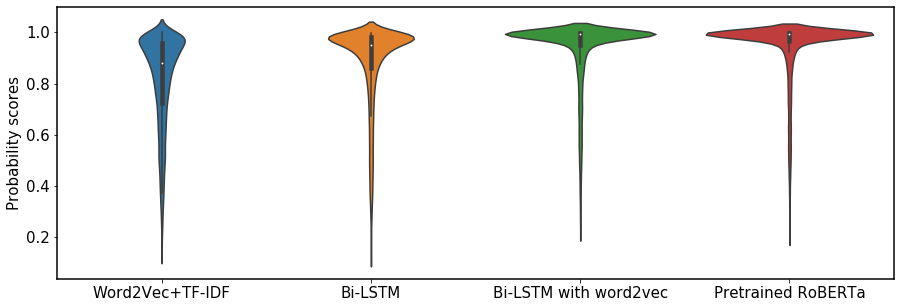
Figure 8. Violin plots of predicted class probability scores for holdout test set for Zone-1 using various approaches.

Type of address	Example	Probable reason
Incomplete	‘House No. XXX, Noida’	Missing locality names
Incoherent	‘Near Kormangala, Hebbal’	Disjoint locality names
Monkey typed	‘dasdasdaasdad’	Fraud/Angry customer

Table 5. Types of misclassified addresses.

RoBERTa based approach, we find that classification errors could be broadly attributed to the categories mentioned in Table 5. Such addresses are hard to interpret even for geo-coding APIs and human evaluators. Our approaches assign a significantly low class probability to such cases and can help in flagging those instances.

9. Conclusion & Future Work

In this paper we tackled the challenging problem of understanding customer addresses in e-commerce for the Indian context. We listed errors commonly made by customers and proposed methodologies to pre-process addresses based on a combination of edit distance and phonetic algorithms. We formulated and compared different approaches based on Word2Vec, Bi-directional LSTM and RoBERTa with respect to sub-region classification task. Evaluation of the approaches is done for North and South Indian addresses on the basis of accuracy scores. We showed that pre-training RoBERTa over a large address dataset and fine-tuning it for classification outperforms other approaches on all the datasets. Pre-training Bi-LSTM based models and using them for downstream task is possible but is slow as compared to BERT variants. Recent research highlights that BERT models are faster to train and capture the context better as compared to Bi-LSTM based models resulting in state-of-the-art-performance on benchmark NLP datasets. This motivated us to use RoBERTa by pre-training it over large address dataset and subsequently fine-tuning it. As part of future work, we can experiment with different tokenization strategies like WordPiece(Devlin et al., 2018) and SentencePiece(Kudo and Richardson, 2018) for tokenizing addresses. We can also pre-train other variants of BERT and compare them based on perplexity score. Such models can generalize better in situations where labelled data is limited like address geo-coding. By framing the problem of parsing address as a language modelling task, this paper presents the first line of research using recent NLP techniques. The deep contextual address embeddings obtained from RoBERTa model can be used to solve multiple problems in the domain of Supply Chain Management.

10. Acknowledgements

The authors would like to thank Nachiappan Sundaram, Deepak Kumar N and Ahsan Mazindrani from Myntra Designs Pvt. Ltd. for their valuable inputs at critical stages of the project.

References

- (1)
- Babu et al. (2015) T. Ravindra Babu, Abhranil Chatterjee, Shivram Khandeparker, A. Vamsi Subhash, and Sawan Gupta. 2015. Geographical address classification without using geolocation coordinates. In Proceedings of the 9th Workshop on Geographic Information Retrieval, GIR 2015, Paris, France, November 26-27, 2015, Ross S. Purves and Christopher B. Jones (Eds.). ACM, 8:1–8:10. https://doi.org/10.1145/2837689.2837696
- Babu and Kakkar (2017) T. Ravindra Babu and Vishal Kakkar. 2017. Address Fraud: Monkey Typed Address Classification for e-Commerce Applications. In eCOM@SIGIR.
- Bokamba (1988) Eyamba G Bokamba. 1988. Code-mixing, language variation, and linguistic theory: Evidence from Bantu languages. Lingua 71, 1 (1988), 21–62.
- Chen et al. (2018) Stanley F Chen, Douglas Beeferman, and Roni Rosenfeld. 2018. Evaluation Metrics For Language Models. https://doi.org/10.1184/R1/6605324.v1
- Craig et al. (2019) Helen Craig, Dragomir Yankov, Renzhong Wang, Pavel Berkhin, and Wei Wu. 2019. Scaling Address Parsing Sequence Models through Active Learning. In Proceedings of the 27th ACM SIGSPATIAL International Conference on Advances in Geographic Information Systems (Chicago, IL, USA) (SIGSPATIAL ’19). Association for Computing Machinery, New York, NY, USA, 424–427. https://doi.org/10.1145/3347146.3359070
- Devlin et al. (2018) Jacob Devlin, Ming-Wei Chang, Kenton Lee, and Kristina Toutanova. 2018. BERT: Pre-training of Deep Bidirectional Transformers for Language Understanding. CoRR abs/1810.04805 (2018). arXiv:1810.04805 http://arxiv.org/abs/1810.04805
- Gevaers et al. (2011) Roel Gevaers, Eddy Van de Voorde, and Thierry Vanelslander. 2011. Characteristics and Typology of Last-mile Logistics from an Innovation Perspective in an Urban Context. In City Distribution and Urban Freight Transport, Cathy Macharis and Sandra Melo (Eds.). Edward Elgar Publishing, Chapter 3. https://ideas.repec.org/h/elg/eechap/14398_3.html
- Gokaslan and Cohen (2019) Aaron Gokaslan and Vanya Cohen. 2019. OpenWebText Corpus. http://Skylion007.github.io/OpenWebTextCorpus
- Hochreiter and Schmidhuber (1997) Sepp Hochreiter and Jürgen Schmidhuber. 1997. Long short-term memory. Neural computation 9, 8 (1997), 1735–1780.
- Howard and Ruder (2018) Jeremy Howard and Sebastian Ruder. 2018. Fine-tuned Language Models for Text Classification. CoRR abs/1801.06146 (2018). arXiv:1801.06146 http://arxiv.org/abs/1801.06146
- Kakkar and Babu (2018) Vishal Kakkar and T. Ravindra Babu. 2018. Address Clustering for e-Commerce Applications. In eCOM@SIGIR.
- Kejriwal and Szekely (2017) Mayank Kejriwal and Pedro Szekely. 2017. Neural Embeddings for Populated Geonames Locations. In The Semantic Web – ISWC 2017, Claudia d’Amato, Miriam Fernandez, Valentina Tamma, Freddy Lecue, Philippe Cudré-Mauroux, Juan Sequeda, Christoph Lange, and Jeff Heflin (Eds.). Springer International Publishing, Cham, 139–146.
- Kingma and Ba (2014) Diederik P. Kingma and Jimmy Ba. 2014. Adam: A Method for Stochastic Optimization. http://arxiv.org/abs/1412.6980 cite arxiv:1412.6980Comment: Published as a conference paper at the 3rd International Conference for Learning Representations, San Diego, 2015.
- Kudo and Richardson (2018) Taku Kudo and John Richardson. 2018. SentencePiece: A simple and language independent subword tokenizer and detokenizer for Neural Text Processing. CoRR abs/1808.06226 (2018). arXiv:1808.06226 http://arxiv.org/abs/1808.06226
- Lai et al. (2017) Guokun Lai, Qizhe Xie, Hanxiao Liu, Yiming Yang, and Eduard Hovy. 2017. RACE: Large-scale ReAding Comprehension Dataset From Examinations. In Proceedings of the 2017 Conference on Empirical Methods in Natural Language Processing. Association for Computational Linguistics, Copenhagen, Denmark, 785–794. https://doi.org/10.18653/v1/D17-1082
- Levenshtein (1966) V. I. Levenshtein. 1966. Binary Codes Capable of Correcting Deletions, Insertions and Reversals. Soviet Physics Doklady 10 (Feb. 1966), 707.
- Ling (1981) Robert F. Ling. 1981. Cluster Analysis Algorithms for Data Reduction and Classification of Objects. Technometrics 23, 4 (1981), 417–418. https://doi.org/10.1080/00401706.1981.10487693 arXiv:https://amstat.tandfonline.com/doi/pdf/10.1080/00401706.1981.10487693
- Liu et al. (2019) Yinhan Liu, Myle Ott, Naman Goyal, Jingfei Du, Mandar Joshi, Danqi Chen, Omer Levy, Mike Lewis, Luke Zettlemoyer, and Veselin Stoyanov. 2019. RoBERTa: A Robustly Optimized BERT Pretraining Approach. CoRR abs/1907.11692 (2019). arXiv:1907.11692 http://arxiv.org/abs/1907.11692
- Loshchilov and Hutter (2017) Ilya Loshchilov and Frank Hutter. 2017. Decoupled Weight Decay Regularization. arXiv:cs.LG/1711.05101
- Mikolov et al. (2013) Tomas Mikolov, Ilya Sutskever, Kai Chen, Greg Corrado, and Jeffrey Dean. 2013. Distributed Representations of Words and Phrases and their Compositionality. (2013).
- Ozdamar and Demir (2012) Linet Ozdamar and Onur Demir. 2012. A hierarchical clustering and routing procedure for large scale disaster relief logistics planning. https://doi.org/10.1016/j.tre.2011.11.003
- Paszke et al. (2019) Adam Paszke, Sam Gross, Francisco Massa, Adam Lerer, James Bradbury, Gregory Chanan, Trevor Killeen, Zeming Lin, Natalia Gimelshein, Luca Antiga, Alban Desmaison, Andreas Kopf, Edward Yang, Zachary DeVito, Martin Raison, Alykhan Tejani, Sasank Chilamkurthy, Benoit Steiner, Lu Fang, Junjie Bai, and Soumith Chintala. 2019. PyTorch: An Imperative Style, High-Performance Deep Learning Library. In Advances in Neural Information Processing Systems 32, H. Wallach, H. Larochelle, A. Beygelzimer, F. d'Alché-Buc, E. Fox, and R. Garnett (Eds.). Curran Associates, Inc., 8024–8035. http://papers.neurips.cc/paper/9015-pytorch-an-imperative-style-high-performance-deep-learning-library.pdf
- Pedregosa et al. (2011) F. Pedregosa, G. Varoquaux, A. Gramfort, V. Michel, B. Thirion, O. Grisel, M. Blondel, P. Prettenhofer, R. Weiss, V. Dubourg, J. Vanderplas, A. Passos, D. Cournapeau, M. Brucher, M. Perrot, and E. Duchesnay. 2011. Scikit-learn: Machine Learning in Python. Journal of Machine Learning Research 12 (2011), 2825–2830.
- Peters et al. (2018) Matthew E. Peters, Mark Neumann, Mohit Iyyer, Matt Gardner, Christopher Clark, Kenton Lee, and Luke Zettlemoyer. 2018. Deep contextualized word representations. In Proc. of NAACL.
- Philips (1990) Lawrence Philips. 1990. Hanging on the Metaphone. Computer Language Magazine 7, 12 (December 1990), 39–44. Accessible at http://www.cuj.com/documents/s=8038/cuj0006philips/.
- Purves and Jones (2011) Ross Purves and Christopher Jones. 2011. Geographic Information Retrieval. SIGSPATIAL Special 3, 2 (July 2011), 2–4. https://doi.org/10.1145/2047296.2047297
- Rajpurkar et al. (2016) Pranav Rajpurkar, Jian Zhang, Konstantin Lopyrev, and Percy Liang. 2016. SQuAD: 100, 000+ Questions for Machine Comprehension of Text. CoRR abs/1606.05250 (2016). arXiv:1606.05250 http://arxiv.org/abs/1606.05250
- Řehůřek and Sojka (2010) Radim Řehůřek and Petr Sojka. 2010. Software Framework for Topic Modelling with Large Corpora. In Proceedings of the LREC 2010 Workshop on New Challenges for NLP Frameworks. ELRA, Valletta, Malta, 45–50.
- Salton and McGill (1986) Gerard Salton and Michael J McGill. 1986. Introduction to modern information retrieval. (1986).
- Sanh et al. (2019) Victor Sanh, Lysandre Debut, Julien Chaumond, and Thomas Wolf. 2019. DistilBERT, a distilled version of BERT: smaller, faster, cheaper and lighter. In NeurIPS EMC2 Workshop.
- Seng (2019) Loke Seng. 2019. A Two-Stage Text-based Approach to Postal Delivery Address Classification using Long Short-Term Memory Neural Networks. (10 2019). https://doi.org/10.13140/RG.2.2.34525.77283
- Sennrich et al. (2015) Rico Sennrich, Barry Haddow, and Alexandra Birch. 2015. Neural Machine Translation of Rare Words with Subword Units. CoRR abs/1508.07909 (2015). arXiv:1508.07909 http://arxiv.org/abs/1508.07909
- Vaswani et al. (2017) Ashish Vaswani, Noam Shazeer, Niki Parmar, Jakob Uszkoreit, Llion Jones, Aidan N. Gomez, Lukasz Kaiser, and Illia Polosukhin. 2017. Attention Is All You Need. CoRR abs/1706.03762 (2017). arXiv:1706.03762 http://arxiv.org/abs/1706.03762
- Vig (2019) Jesse Vig. 2019. A Multiscale Visualization of Attention in the Transformer Model. In Proceedings of the 57th Conference of the Association for Computational Linguistics, ACL 2019, Florence, Italy, July 28 - August 2, 2019, Volume 3: System Demonstrations, Marta R. Costa-jussà and Enrique Alfonseca (Eds.). Association for Computational Linguistics, 37–42. https://doi.org/10.18653/v1/p19-3007
- Wang et al. (2018) Alex Wang, Amanpreet Singh, Julian Michael, Felix Hill, Omer Levy, and Samuel Bowman. 2018. GLUE: A Multi-Task Benchmark and Analysis Platform for Natural Language Understanding. In Proceedings of the 2018 EMNLP Workshop BlackboxNLP: Analyzing and Interpreting Neural Networks for NLP. Association for Computational Linguistics, Brussels, Belgium, 353–355. https://doi.org/10.18653/v1/W18-5446
- Wolf et al. (2019) Thomas Wolf, Lysandre Debut, Victor Sanh, Julien Chaumond, Clement Delangue, Anthony Moi, Pierric Cistac, Tim Rault, Rémi Louf, Morgan Funtowicz, and Jamie Brew. 2019. HuggingFace’s Transformers: State-of-the-art Natural Language Processing. arXiv:cs.CL/1910.03771