On the Validity of Physical Optics for Narrow-band Beam Scattering and Diffraction from the Open Cylindrical Surface

F. M. Lastname

F. M. Lastname

Abstract— The exact formulas for the induced electric surface current (in the scattering phenomenon) and the equivalent electric surface current (in the diffraction phenomenon) on the open cylindrical surface due to an arbitrary narrow-band beam have been shown in their closed-form expressions within the context of the cylindrical harmonics, which gives information about the validity of the Physical Optics (PO) approximation. Both the Electric Field Integral Equation (EFIE) and the Magnetic Field Integral Equation (MFIE) are used to find the induced (equivalent) electric surface currents in the context of the cylindrical harmonics. The numerical example of the scattering and diffraction of the Hermite Gaussian beam from the open cylindrical surface is shown. The result is useful for the evaluation of the validity of the PO approximation in the cylinder-like surface.

I. Introduction

The Physical Optics (PO) approximation has been extensively used as the approximation of the exact solution in many applications [1, 2, 3, 4, 5, 6, 7, 8, 9, 10, 11, 12, 13, 14, 15, 16, 17], which include microwave imaging, reflector antenna design, and evaluation of Radar Cross Section (RCS) [18, 19, 20, 21]. It is helpful to have an analytical formula to predict the behavior of the PO approximation in order to use it effectively. In this article, the exact closed-form expressions will be shown for the induced (equivalent) electric surface currents on the open cylindrical surface, from which the information of the validity of the PO approximation is obtained for the cylinder-like surface. The scheme used to illustrate the problem is given in Fig. 1. The time dependence $e^{i\omega t}$ ($i=\sqrt{-1}$) has been assumed in this article.

II. The Cylindrical Harmonics

The cylindrical modal expansion of the vector potential ${\bf A}({\bf r})$ for the electric surface current ${\bf J}_{s}({\bf r}^{\prime})$ on an arbitrary surface in the cylindrical coordinate is given as

$${\bf A}({\bf r})=\mu\int\!\!\int_{S}\left[\begin{array}[]{cccc}\\ \\ \end{array}g({\bf r-r^{\prime}}){\bf J}_{s}{\bf(r^{\prime})}\begin{array}[]{cccc}\\ \\ \end{array}\right]dS^{\prime}=\frac{\mu}{i8\pi}\int\!\!\int_{S}\left[\begin{array}[]{cccc}\\ \\ \end{array}{\bf J}_{s}{\bf(r^{\prime})}\int_{-\infty}^{\infty}H_{0}^{(2)}\left(\Lambda\left|\boldsymbol{\rho}-\boldsymbol{\rho}^{\prime}\right|\right)e^{-ih(z-z^{\prime})}dh\begin{array}[]{cccc}\\ \\ \end{array}\right]dS^{\prime}$$ (9)

where $\mu$ is the permeability of the homogeneous medium. $H_{0}^{(2)}(\ {\cdot}\ )$ is Hankel function of the second kind of order 0. The scalar Green’s function $g(\ \cdot\ )$ and the transverse wave vector $\Lambda$ are defined as

$$g(\ {\cdot}\ )=\frac{e^{-ik|\ {\cdot}\ |}}{4\pi|\ {\cdot}\ |},\ \ \Lambda=\sqrt{k^{2}-h^{2}}.$$ (10)

According to the cylindrical addition theorem,

$$H_{0}^{(2)}\left(\Lambda\left|\boldsymbol{\rho}-\boldsymbol{\rho}^{\prime}\right|\right)=\sum_{m=-\infty}^{\infty}\left\{\begin{array}[]{ccc}\left.H_{m}^{(2)}(\Lambda\rho)J_{m}(\Lambda\rho^{\prime})e^{im(\phi^{\prime}-\phi)}\right|_{\rho>\rho^{\prime}}\\ \\ \left.J_{m}(\Lambda\rho)H_{m}^{(2)}(\Lambda\rho^{\prime})e^{im(\phi^{\prime}-\phi)}\right|_{\rho<\rho^{\prime}}\end{array}\right.\hskip 14.45377pt$$ (14)

where $\rho\equiv|\boldsymbol{\rho}|$ is the observation coordinate and $\rho^{\prime}\equiv|\boldsymbol{\rho}^{\prime}|$ is the source coordinate. $J_{m}(\ {\cdot}\ )$ is Bessel function of the first kind of integer order $m$ and $H_{m}^{(2)}(\ {\cdot}\ )$ is Hankel function of the second kind of integer order $m$. Substituting (14) into (9), the cylindrical modal expansion of ${{\bf A}({\bf r})}$ is obtained,

$${\bf A}^{>}_{<}({\bf r}) = \hbox{IFT}\left({\bf g}^{>}_{<}(m,h)\begin{array}[]{cc}H_{m}^{(2)}(\Lambda\rho)\\ J_{m}(\Lambda\rho)\end{array}\begin{array}[]{cccc}\\ \\ \end{array}\right)$$ (19)

$$\ \ \ \ \ \ \ \ {\bf g}^{>}_{<}(m,h)=\frac{\mu}{i4}\int\!\!\int_{S}\left[\begin{array}[]{cc}J_{m}(\Lambda\rho^{\prime})\\ H_{m}^{(2)}(\Lambda\rho^{\prime})\end{array}{\bf J}_{s}{\bf(r^{\prime})}e^{i(m\phi^{\prime}+hz^{\prime})}\begin{array}[]{cccc}\\ \\ \end{array}\right]dS^{\prime}$$ (24)

where, the the superscript “$>$” denotes $\rho>\rho^{\prime}$ and the subscript “$<$” denotes $\rho<\rho^{\prime}$. The Inverse Fourier Transform (IFT) is defined as

$$\hbox{IFT}\left(\begin{array}[]{ccc}\\ \end{array}{\cdot}\begin{array}[]{ccc}\\ \end{array}\right)=\frac{1}{2\pi}\sum_{m=-\infty}^{\infty}\left\{\int_{-\infty}^{\infty}\left[\left(\begin{array}[]{ccc}\\ \end{array}{\cdot}\begin{array}[]{ccc}\\ \end{array}\right)e^{-i(m\phi+hz)}\begin{array}[]{ccc}\\ \end{array}\right]dh\begin{array}[]{ccc}\\ \\ \\ \end{array}\right\}.$$ (25)

The electromagnetic field (${\bf E},{\bf H}$) is given as

$${\bf E}^{>}_{<}({\bf r})=-i\omega{\bf A}^{>}_{<}({\bf r})+\frac{1}{i\omega\mu\epsilon}\nabla\left[\nabla\cdot{\bf A}^{>}_{<}({\bf r})\begin{array}[]{ccc}\\ \\ \end{array}\right],\ \ \ \ {\bf H}^{>}_{<}({\bf r})=\frac{1}{\mu}\nabla\times{\bf A}^{>}_{<}({\bf r})$$ (26)

Figure 1: The narrow-band beam scattering and diffraction in the cylindrical geometry: the incident field ${\bf E}^{i}$ propagates onto cylindrical surface $S$ with radius of $\rho_{0}$, then it could be back-scattered to ${\bf E}^{s}$ if surface $S$ serves as a PEC scatter, with induced surface current ${\bf J}_{s}^{-}$; or it may forward-propagate to ${\bf E}^{d}$ if it is a diffraction phenomenon, with equivalent surface current ${\bf J}_{s}^{+}=-{\bf J}_{s}^{-}$. $\hat{\bf n}^{+}$ and $\hat{\bf n}^{-}$ are the outward and inward unit surface normals to $S$ respectively.

III. Exact Formulas for Induced and Equivalent Electric Surface Currents

Due to the fact that ${\bf J}_{s}^{-}=-{\bf J}_{s}^{+}$ (see Fig. 1), let’s consider the scattering phenomenon and express the incident electromagnetic field (${\bf E}^{i},{\bf H}^{i}$) into the cylindrical harmonics,

$${\bf E}^{i}(\rho)=\sum_{m=-\infty}^{\infty}\left\{\int_{-\infty}^{\infty}\left[\begin{array}[]{ccc}\\ \\ \end{array}a^{h}_{m}\ {\bf M}^{h}_{m}(\rho)+b^{h}_{m}\ {\bf N}^{h}_{m}(\rho)\begin{array}[]{ccc}\\ \\ \end{array}\right]dh\begin{array}[]{ccc}\\ \\ \\ \end{array}\right\}$$ (34)

$${\bf H}^{i}(\rho)=\frac{i}{\eta}\sum_{m=-\infty}^{\infty}\left\{\int_{-\infty}^{\infty}\left[\begin{array}[]{ccc}\\ \\ \end{array}a^{h}_{m}\ {\bf N}^{h}_{m}(\rho)+b^{h}_{m}\ {\bf M}^{h}_{m}(\rho)\begin{array}[]{ccc}\\ \\ \end{array}\right]dh\begin{array}[]{ccc}\\ \\ \\ \end{array}\right\}$$ (42)

$${\bf M}^{h}_{m}({\bf r})=\left[\begin{array}[]{ccc}\\ \\ \end{array}\hat{\boldsymbol{\rho}}\frac{m}{i\rho}H_{m}^{(2)}(\Lambda\rho)-\hat{\boldsymbol{\phi}}\Lambda\frac{\partial H_{m}^{(2)}(\Lambda\rho)}{\partial(\Lambda\rho)}\begin{array}[]{ccc}\\ \\ \end{array}\right]e^{-im\phi}e^{-ihz}$$ (47)

$${\bf N}^{h}_{m}({\bf r})=\left[\begin{array}[]{ccc}\\ \\ \end{array}\hat{\boldsymbol{\rho}}\frac{h\Lambda}{ik}\frac{\partial H_{m}^{(2)}(\Lambda\rho)}{\partial(\Lambda\rho)}-\hat{\boldsymbol{\phi}}\frac{mh}{k\rho}H_{m}^{(2)}(\Lambda\rho)+\hat{\bf z}\frac{\Lambda^{2}}{k}H_{m}^{(2)}(\Lambda\rho)\begin{array}[]{ccc}\\ \\ \end{array}\right]e^{-im\phi}e^{-ihz}$$ (52)

Similarly, express the scattered electromagnetic field (${\bf E}^{s},{\bf H}^{s}$) as

$${\bf E}^{s}(\rho)=\sum_{m=-\infty}^{\infty}\left\{\int_{-\infty}^{\infty}\left[\begin{array}[]{ccc}\\ \\ \end{array}c^{h}_{m}\ {\bf M}^{h}_{m}(\rho)+d^{h}_{m}\ {\bf N}^{h}_{m}(\rho)\begin{array}[]{ccc}\\ \\ \end{array}\right]dh\begin{array}[]{ccc}\\ \\ \\ \end{array}\right\}$$ (60)

$${\bf H}^{s}(\rho)=\frac{i}{\eta}\sum_{m=-\infty}^{\infty}\left\{\int_{-\infty}^{\infty}\left[\begin{array}[]{ccc}\\ \\ \end{array}c^{h}_{m}\ {\bf N}^{h}_{m}(\rho)+d^{h}_{m}\ {\bf M}^{h}_{m}(\rho)\begin{array}[]{ccc}\\ \\ \end{array}\right]dh\begin{array}[]{ccc}\\ \\ \\ \end{array}\right\}$$ (68)

Now the induced electric surface current ${\bf J}_{s}^{-}$ on the cylindrical surface $S$ is given as

$${\bf J}_{s}^{-}(\rho_{0})=\hat{\bf n}^{-}\times\left[{\bf H}^{i}(\rho_{0})+{\bf H}^{s}(\rho_{0})\right]=\left[{\bf H}^{i}(\rho_{0})+{\bf H}^{s}(\rho_{0})\right]\times\hat{\boldsymbol{\rho}}_{0}$$ (69)

$$=\frac{i}{\eta}\sum_{m=-\infty}^{\infty}\left\{\int_{-\infty}^{\infty}\left[\begin{array}[]{ccc}\\ \\ \end{array}\left(a^{h}_{m}+c^{h}_{m}\right){\bf N}^{h}_{m}(\rho_{0})\times\hat{\boldsymbol{\rho}}_{0}+\left(b^{h}_{m}+d^{h}_{m}\right){\bf M}^{h}_{m}(\rho_{0})\times\hat{\boldsymbol{\rho}}_{0}\begin{array}[]{ccc}\\ \\ \end{array}\right]dh\begin{array}[]{ccc}\\ \\ \\ \end{array}\right\}$$ (77)

1.  Electric Field Integral Equation (EFIE)

Let’s consider the TM mode (${\bf N}^{h}_{m}$ for ${\bf E}$ and ${\bf M}^{h}_{m}$ for ${\bf H}$) here. From (47) and (69),

$${\bf J}_{s}^{-,\hbox{\tiny TM}}(\rho_{0})=\hat{\bf z}\frac{i}{\eta}\sum_{m=-\infty}^{\infty}\left\{\begin{array}[]{ccc}\\ \\ \\ \end{array}\int_{-\infty}^{\infty}\left(b^{h}_{m}+d^{h}_{m}\right)\Lambda\left.\frac{\partial H_{m}^{(2)}(\Lambda\rho)}{\partial(\Lambda\rho)}\right|_{\rho_{0}}dh\begin{array}[]{ccc}\\ \\ \\ \end{array}\right\}$$ (84)

Substituting (84) into (26), the $z$-component of the scattered electric field $\hbox{ E}^{s,\hbox{\tiny TM}}_{z,<}$ on the cylindrical surface is obtained ($\hbox{A}_{z,<}^{\hbox{\tiny TM}}\equiv\hat{\bf z}\cdot{\bf A}_{<}^{\hbox{\tiny TM}}$),

$$\hbox{ E}^{s,\hbox{\tiny TM}}_{<,z}(\rho_{0})=-i\omega\left(\frac{\Lambda}{k}\right)^{2}\hbox{A}_{z,<}^{\hbox{\tiny TM}}(\rho_{0})$$ (85)

$$=\frac{\pi\rho_{0}}{i2k}\sum_{m=-\infty}^{\infty}\left\{\begin{array}[]{ccc}\\ \\ \\ \end{array}\int_{-\infty}^{\infty}\left(b^{h}_{m}+d^{h}_{m}\right)\Lambda^{3}J_{m}(\Lambda\rho_{0})H_{m}^{(2)}(\Lambda\rho_{0})\left.\frac{\partial H_{m}^{(2)}(\Lambda\rho)}{\partial(\Lambda\rho)}\right|_{\rho_{0}}dh\begin{array}[]{ccc}\\ \\ \\ \end{array}\right\}$$ (92)

Note that $\hbox{ E}^{s,\hbox{\tiny TM}}_{z,<}$ is given on the whole cylindrical surface that is just inside (infinitesimally close to) cylindrical surface $S$, on both the front side and the back side. It can be separated into two parts for the narrow-band beam, which can be seen from the property of Bessel function,

$$J_{m}(\ \cdot\ )=\frac{H_{m}^{(1)}(\ \cdot\ )+H_{m}^{(2)}(\ \cdot\ )}{2}$$ (93)

The scattered electric field on the front side is thus given as

$$\hbox{ E}^{s,\hbox{\tiny TM}}_{z,<,f}(\rho_{0})=\frac{\pi\rho_{0}}{i4k}\sum_{m=-\infty}^{\infty}\left\{\begin{array}[]{ccc}\\ \\ \\ \end{array}\int_{-\infty}^{\infty}\left(b^{h}_{m}+d^{h}_{m}\right)\Lambda^{3}H_{m}^{(1)}(\Lambda\rho_{0})H_{m}^{(2)}(\Lambda\rho_{0})\left.\frac{\partial H_{m}^{(2)}(\Lambda\rho)}{\partial(\Lambda\rho)}\right|_{\rho_{0}}dh\begin{array}[]{ccc}\\ \\ \\ \end{array}\right\}$$ (100)

Now apply the EFIE on the cylindrical surface $\hbox{E}^{s,\hbox{\tiny TM}}_{z,<,f}(\rho_{0})=-\hbox{E}^{i,\hbox{\tiny TM}}_{z}(\rho_{0})$, from (34) and (100),

$$b^{h}_{m}+d^{h}_{m}=\frac{2}{\xi}b^{h}_{m},\ \ \ \ \ d^{h}_{m}=\left[\frac{2}{\xi}-1\right]b^{h}_{m},\ \ \ \ \ \xi\equiv i\frac{\pi}{2}\Lambda\rho_{0}H_{m}^{(1)}(\Lambda\rho_{0})\left.\frac{\partial H_{m}^{(2)}(\Lambda\rho)}{\partial(\Lambda\rho)}\right|_{\rho_{0}}$$ (101)

Note that $\xi\rightarrow 1$ for $\rho_{0}\rightarrow\infty$, which means that $d^{h}_{m}\rightarrow b^{h}_{m}$ and the PO approximation reduces to the exact induced electric surface current.

2.  Magnetic Field Integral Equation (MFIE)

Let’s also take the TM mode (${\bf N}^{h}_{m}$ for ${\bf E}$ and ${\bf M}^{h}_{m}$ for ${\bf H}$) as an example. From (26) and (84), the $\phi$-component of the scattered magnetic field $\hbox{ H}^{s,\hbox{\tiny TM}}_{\phi,<,f}(\rho_{0})$ on the front side of the cylindrical surface is found as

$$\hbox{ H}^{s,\hbox{\tiny TM}}_{\phi,<,f}(\rho_{0})=\frac{i}{\eta}\sum_{m=-\infty}^{\infty}\left\{\int_{-\infty}^{\infty}\left[\begin{array}[]{ccc}\\ \\ \end{array}\frac{\xi^{\ast}}{2}\left(b^{h}_{m}+d^{h}_{m}\right)\ {\bf M}^{h}_{m}(\rho)\begin{array}[]{ccc}\\ \\ \end{array}\right]dh\begin{array}[]{ccc}\\ \\ \\ \end{array}\right\}$$ (109)

Now apply the MFIE on the cylindrical surface $\hbox{ H}^{s,\hbox{\tiny TM}}_{\phi,<,f}(\rho_{0})+\hbox{ H}^{i,\hbox{\tiny TM}}_{\phi}(\rho_{0})=-\hbox{J}_{s,z}^{-,\hbox{\tiny TM}}(\rho_{0})$,

$$b^{h}_{m}+d^{h}_{m}=\frac{2}{2-\xi^{\ast}}b^{h}_{m},\ \ \ \ \ d^{h}_{m}=\frac{\xi^{\ast}}{2-\xi^{\ast}}b^{h}_{m}$$ (110)

It is not difficult to show that (101) and (110) are equivalent by using the Wronskian relation,

$$H_{m}^{(2)}(\Lambda\rho)\frac{\partial H_{m}^{(1)}(\Lambda\rho)}{\partial(\Lambda\rho)}-H_{m}^{(1)}(\Lambda\rho)\frac{\partial H_{m}^{(2)}(\Lambda\rho)}{\partial(\Lambda\rho)}=\frac{i4}{\pi\Lambda\rho}$$ (111)

3. The Induced and Equivalent Electric Surface Currents

Following the similar procedure, the induced electric surface current for the TE mode (${\bf M}^{h}_{m}$ for ${\bf E}$ and ${\bf N}^{h}_{m}$ for ${\bf H}$) is given as

$$a^{h}_{m}+c^{h}_{m}=\frac{2}{\xi^{\ast}}a^{h}_{m},\ \ \ \ \ c^{h}_{m}=\left[\frac{2}{\xi^{\ast}}-1\right]a^{h}_{m}$$ (112)

Substituting (101) and (112) into (69), the total induced and equivalent electric surface currents are obtained,

$${\bf J}_{s}^{-}(\rho_{0})=-{\bf J}_{s}^{+}(\rho_{0})=\frac{i2}{\eta}\sum_{m=-\infty}^{\infty}\left\{\int_{-\infty}^{\infty}\left[\begin{array}[]{ccc}\\ \\ \end{array}a_{m}^{h}\frac{{\bf N}^{h}_{m}(\rho_{0})\times\hat{\boldsymbol{\rho}}_{0}}{\xi^{\ast}}+b_{m}^{h}\frac{{\bf M}^{h}_{m}(\rho_{0})\times\hat{\boldsymbol{\rho}}_{0}}{\xi}\begin{array}[]{ccc}\\ \\ \end{array}\right]dh\begin{array}[]{ccc}\\ \\ \\ \end{array}\right\}$$ (120)

From (120), it is clear that the exact induced and equivalent electric surface currents only deviate from the PO approximation by a factor of $\frac{1}{\xi}$ for TM mode and $\frac{1}{\xi^{\ast}}$ for TE mode.

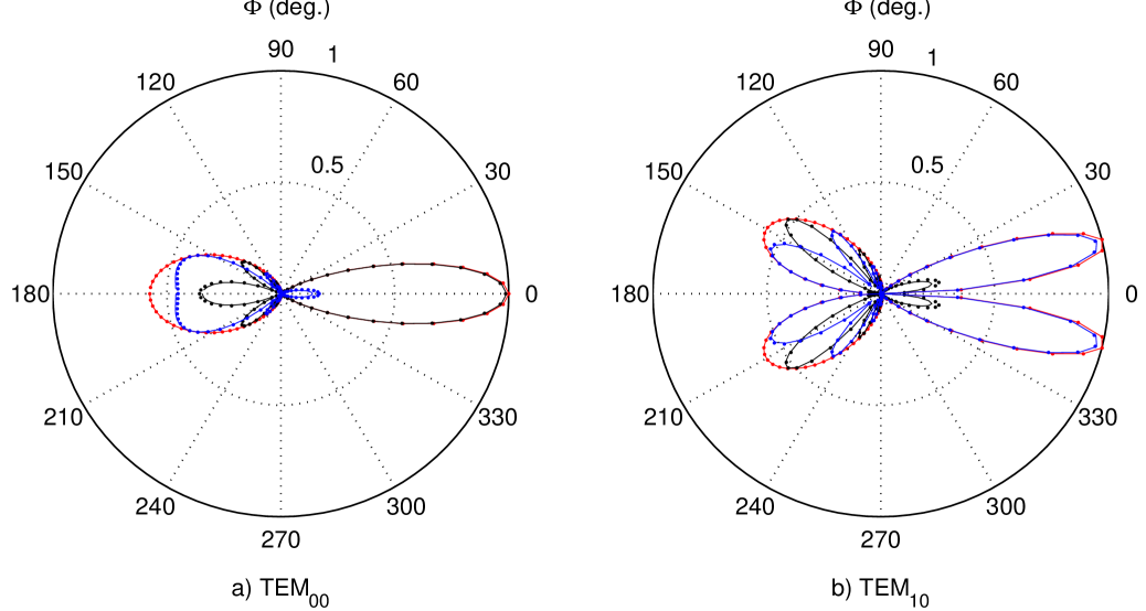
Figure 2: The PO approximation (dots) Vs. result (lines) from MoM: a) TEM₀₀; and b) TEM₁₀. Red is for the magnitude; blue is for the real part; and black is for the imaginary part. Results have been normalized.

IV. Numerical Confirmation: the Hermite Gaussian Beam

The incident Hermite Gaussian beam (TEM₀₀ and TEM₁₀) has been used to test the result given in (120). The TEM_mn Hermite Gaussian beam is given as

$${\bf E}_{mn}=\hat{\bf z}\sqrt{\frac{\eta}{\pi 2^{m+n-2}m!n!w_{y}(x)w_{z}(x)}}\hbox{H}_{m}\left(\sqrt{2}\frac{y}{w_{y}(x)}\right)\hbox{H}_{n}\left(\sqrt{2}\frac{z}{w_{z}(x)}\right)$$ (121)

$$e^{-\left[y^{2}\left(\frac{1}{w_{y}^{2}(x)}+\frac{ik}{2R_{y}(x)}\right)+z^{2}\left(\frac{1}{w_{z}^{2}(x)}+\frac{ik}{2R_{z}(x)}\right)\right]}e^{-i\left[kx-\left(m+\frac{1}{2}\right)\arctan\left(\frac{x}{\hbox{\tiny L}_{y}}\right)-\left(n+\frac{1}{2}\right)\arctan\left(\frac{x}{\hbox{\tiny L}_{z}}\right)\right]},$$

where H_m,n is the Hermite polynomial and the following quantities have been defined,

$$w_{\tau}(x)=w_{0\tau}\left[1+\frac{x}{\hbox{\small L}_{\tau}}\right]^{\frac{1}{2}},\ \ \ \ R_{\tau}(x)=x+\hbox{L}_{\tau}^{2}/x,\ \ \ \ \hbox{L}_{\tau}=\frac{kw_{0\tau}^{2}}{2},\ \ \ \ \tau=y,z$$ (122)

In our numerical computation, both TEM₀₀ and TEM₁₀ Hermite Gaussian beams are $\hat{\bf z}$-polarized (TM mode only in the cylindrical coordinate). The symmetrical waist radii have been set as $w_{0y}=w_{0z}=1\lambda$. The radius of the scattering (diffracting) cylindrical surface is $\rho_{0}=3\lambda$ and the radius of the observation cylindrical surface is $\rho=20\lambda$.

The scattered electric field $\hbox{E}_{z}^{s}$ ($\phi\in\left[\frac{\pi}{2},\frac{3\pi}{2}\right]$) and the diffracted electric field $\hbox{E}_{z}^{d}$ ($\phi\in\left[-\frac{\pi}{2},\frac{\pi}{2}\right]$) calculated from the PO approximation have been plotted (dots) in Fig. 2, together with the result (lines) obtained from the Method of Moment (MoM). Also, the theoretical induced (equivalent) current given in (120) has been used to calculate the scattered electric field $\hbox{E}_{z}^{s}$ and the diffracted electric field $\hbox{E}_{z}^{d}$, which is shown in Fig. 3 (dots), with good agreement with the result from the MoM (lines). All plots are for results on the observation cylindrical surface with radius $\rho=20\lambda$.

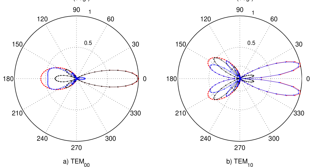
Figure 3: Result (dots) obtained from Eqn. (120) Vs. result (lines) from MoM: a) TEM₀₀ and b) TEM₁₀. Red is for the magnitude; blue is for the real part; and black is for the imaginary part. Results have been normalized.

Conclusion

The exact formulas for the induced electric surface current in the scattering phenomenon and the equivalent electric surface current in the diffraction phenomenon have been derived, which gives helpful information of the PO approximation in the cylinder-like surface.

Bibliography

• [1] Shaolin Liao and Ronald J. Vernon, “The Near-Field and Far-Field Properties of the Cylindrical Modal Expansions with Application in the Image Theorem,” In 2006 Joint 31st International Conference on Infrared Millimeter Waves and 14th International Conference on Teraherz Electronics, pages 260-260, September 2006. ISSN: 2162-2035.
• [2] Shaolin Liao and R.J. Vernon, “A new fast algorithm for calculating near-field propagation between arbitrary smooth surfaces,” In 2005 Joint 30th International Conference on Infrared and Millimeter Waves and 13th International Conference on Terahertz Electronics, volume 2, pages 606-607 vol. 2, September 2005. ISSN: 2162-2035.
• [3] Shaolin Liao, Henry Soekmadji, and Ronald J. Vernon, “On Fast Computation of Electromagnetic Wave Propagation through FFT,” In 2006 7th International Symposium on Antennas Propagation EM Theory, pages 1-4, October 2006.
• [4] Shaolin Liao and Ronald J. Vernon, “The Cylindrical Taylor-Interpolation FFT Algorithm,” In 2006 Joint 31st International Conference on Infrared Millimeter Waves and 14th International Conference on Teraherz Electronics, pages 259-259, September 2006. ISSN: 2162-2035.
• [5] Shaolin Liao, “Beam-shaping PEC Mirror Phase Corrector Design,” PIERS Online, 3(4):392-396, 2007.
• [6] Shaolin Liao, “Fast Computation of Electromagnetic Wave Propagation and Scattering for Quasi-cylindrical Geometry,” PIERS Online, 3(1):96-100, 2007.
• [7] Shaolin Liao, “On the Validity of Physical Optics for Narrow-band Beam Scattering and Diffraction from the Open Cylindrical Surface,” PIERS Online, 3(2):158-162, 2007.
• [8] Shaolin Liao, Ronald J. Vernon, and Jeffrey Neilson, “A high-efficiency four-frequency mode converter design with small output angle variation for a step-tunable gyrotron,” In 2008 33rd International Conference on Infrared, Millimeter and Terahertz Waves, pages 1-2, September 2008. ISSN: 2162-2035.
• [9] S. Liao, R. J. Vernon, and J. Neilson, “A four-frequency mode converter with small output angle variation for a step-tunable gyrotron,” In Electron Cyclotron Emission and Electron Cyclotron Resonance Heating (EC-15), pages 477-482. WORLD SCIENTIFIC, April 2009.
• [10] Ronald J. Vernon, “High-Power Microwave Transmission and Mode Conversion Program,” Technical Report DOEUW52122, Univ. of Wisconsin, Madison, WI (United States), August 2015.
• [11] Shaolin Liao, Multi-frequency beam-shaping mirror system design for high-power gyrotrons: theory, algorithms and methods, Ph.D. Thesis, University of Wisconsin at Madison, USA, 2008. AAI3314260 ISBN-13: 9780549633167.
• [12] Shaolin Liao and Ronald J. Vernon, “A Fast Algorithm for Wave Propagation from a Plane or a Cylindrical Surface,” International Journal of Infrared and Millimeter Waves, 28(6):479-490, June 2007.
• [13] S.-L. Liao and R. J. Vernon, “Sub-THz Beam-Shaping Mirror System Designs for Quasi-optical Mode Converters in High-power Gyrotrons,” Journal of Electromagnetic Waves and Applications, 21(4):425-439, January 2007. Publisher: Taylor & Francis.
• [14] Shaolin Liao, “Miter Bend Mirror Design for Corrugated Waveguides,” Progress In Electromagnetics Research, 10:157-162, 2009.
• [15] Shaolin Liao and Ronald J. Vernon, “A Fast Algorithm for Computation of Electromagnetic Wave Propagation in Half-Space,” IEEE Transactions on Antennas and Propagation, 57(7):2068-2075, July 2009.
• [16] Shaolin Liao, N. Gopalsami, A. Venugopal, A. Heifetz, and A. C. Raptis, “An efficient iterative algorithm for computation of scattering from dielectric objects,” Optics Express, 19(4):3304-3315, February 2011. Publisher: Optical Society of America.
• [17] Shaolin Liao, “Spectral-domain MOM for Planar Meta-materials of Arbitrary Aperture Wave-guide Array,” In 2019 IEEE MTT-S International Conference on Numerical Electromagnetic and Multiphysics Modeling and Optimization (NEMO), pages 1-4, May 2019.
• [18] D-B Lin and T-H Chu, “Bistatic frequency-swept microwave imaging: principle, methodology and experimental results,” IEEE Transactions on Microwave Theory and Techniques, Vol. 41, No. 5, May 1993, pp. 855-861.
• [19] B. Schlobohm, F. Amdt and J. Kless, “Direct PO optimized dual-offset reflector antennas for small earth stations and for millimeter wave atmospheric sensors,” IEEE Transactions on Microwave Theory and Techniques, Vol. 40, No. 6, June 1992, pp. 1310-1317.
• [20] T. J. Hestilow, “Simple formulas for the calculation of the average physical optics RCS of a cylinder and a flat plate over a symmetric window around broadside,” IEEE Antennas and Propagation Magazine, Vol. 42, No. 5, Oct. 2000, pp. 48-52.
• [21] Shaolin Liao and R. J. Vernon, “A new fast algorithm for field propagation between arbitrary smooth surfaces”, In: the joint 30${}^{\hbox{\tiny th}}$ Infrared and Millimeter Waves and 13${}^{\hbox{\tiny th}}$ International Conference on Terahertz Electronics, Williamsburg, Virginia, USA, 2005, ISBN: 0-7803-9348-1, INSPEC number: 8788764, DOI: 10.1109/ICIMW.2005.1572687, Vol. 2, pp. 606-607.