Beam-Shaping PEC Mirror Phase Corrector Design

F. M. Lastname

F. M. Lastname

Abstract— The Perfect Electric Conductor (PEC) mirror phase corrector plays an important role in the beam-shaping mirror system design for Quasi-Optical (QO) mode converter (launcher) in the sub-THz high-power gyrotron. In this article, both the Geometry Optical (GO) method and the phase gradient method have been presented for the PEC mirror phase corrector design. The advantages and disadvantages are discussed for both methods. An efficient algorithm has been proposed for the phase gradient method.

The PEC mirror phase corrector is essential to shape the input beam from the QO mode converter (launcher) into the desired Fundamental Gaussian Beam (FGB) in the sub-THz high-power gyrotron [1, 2, 3, 4, 5, 6, 7, 8, 9, 10, 11, 12, 13, 14, 15, 16, 17, 18, 19, 20]. Figure 1 shows the diagram of such beam-shaping mirror system, in which the 4 pieces of PEC mirrors (M₁, M₂, M₃ and M₄) serve as the phase correctors, aiming at shaping the input beam from the QO launcher into the desired FGB output beam. During the iterative beam-shaping mirror system design [1, 6], phase unwrapping is commonly required in the PEC mirror phase corrector design, which can effectively suppress the edge diffraction due to the discontinuities if otherwise the wrapped phase is used. In this article, both the GO method and the phase gradient method are discussed. An FFT-based efficient algorithm is also proposed to speed up the PEC mirror phase corrector design for the phase gradient method. The time dependence $e^{i\omega t}$ is assumed.

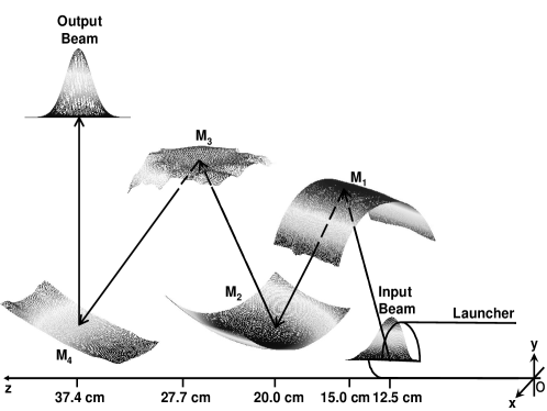
Figure 1: The diagram of the beam-shaping mirror system consisting of 4 pieces of PEC mirrors to shape the input beam from the QO launcher into the desired FGB output beam. The approximate z coordinates of the 4 pieces of PEC mirrors have been marked on z axis.

II. The Problem of Phase Unwrapping

The phase correction requires the knowledge of the unwrapped 2-Dimensional (2D) phases of the incident electric field and the reflected electric field ($\theta^{i}$, $\theta^{r}$). However, the phase obtained from the electric field E through $\check{\theta}=\arctan\left[\frac{\Im({\bf E})}{\Re({\bf E})}\right]$ ($\Re$ and $\Im$ denote the real part and the imaginary part respectively) is the wrapped 2D phase, which contains discontinuities of $2n\pi$ (n is an integer). So, in order to ensure the smoothness of the PEC mirror surface, the wrapped 2D phases ($\check{\theta}^{i}$, $\check{\theta}^{r}$) must be unwrapped through the 2D phase unwrapping methods [21, 22].

Mathematically, in the ideal situation where there is no residues in the wrapped 2D phase $\check{\theta}$, the discreet phase gradient $\nabla{\theta}=\nabla\check{\theta}$ (assuming that $\nabla{\theta}<\pi$) and the 2D phase unwrapping can be expressed as,

$$\theta=\int_{C}\nabla\check{\theta}\cdot d{\bf r}+\theta({\bf r}_{0})$$ (1)

where, $\theta$ denotes the 2D unwrapped phase along the integration path $C$ and $r_{0}$ denotes the starting point of the path integration. Note that the unwrapped phase $\theta$ obtained through (1) should not depend on the integration path $C$. However, due to the residues in practice, the discrete phase gradient should be written as $\nabla\check{\theta}=(\nabla g+\nabla\times{\bf R})$ and the unwrapped phase $\theta$ is obtained as follows,

$$\theta=\int_{C}(\nabla g+\nabla\times{\bf R})\cdot d{\bf r}+\theta({\bf r}_{0})$$ (2)

From (2), it can be seen that $\nabla\times{\bf R}\neq 0$ is caused by the existence of residues and the unwrapped phase $\theta$ depends on the integration path $C$. There are many 2D phase unwrapping algorithms to deal with the residues in the literatures [21], [22]. For example, the path following algorithm (e.g., “quality-guided” method and “mask-cut” method) gives faithful congruent unwrapped phase (with $2n\pi$ difference from the wrapped phase). However, path following algorithm is time-consuming and the unwrapped phase contains many discontinuities due to the existence of residues. Another commonly-used algorithm, the minimum norm method unwraps the wrapped phase by minimizing the $r$-norm phase difference between the gradients of the wrapped phase and the desired unwrapped phase [22],

$$Q=\sum_{X}\sum_{Z}\left[\begin{array}[]{cccc}\\ \\ \\ \end{array}w_{x}\left|\frac{\partial\theta}{\partial x}-\frac{\partial\check{\theta}}{\partial x}\right|^{r}+w_{z}\left|\frac{\partial\theta}{\partial z}-\frac{\partial\check{\theta}}{\partial z}\right|^{r}\begin{array}[]{cccc}\\ \\ \\ \end{array}\right]$$ (9)

where, $w_{x}$ and $w_{z}$ are weights for $\hat{\bf x}$ and $\hat{\bf z}$ directions respectively. When $r=2$, it is called the Least Mean Square (LMS) method.

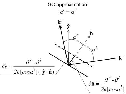
Figure 2: The PEC mirror surface correction in the sub-THz QO regime: ${\bf k}^{i}$ and ${\bf k}^{r}$ are wave vectors for the local incident beam (with incident angle $\alpha^{i}$) and the local reflection beam (with reflected angle $\alpha^{r}$). $\delta_{\hat{\bf n}}$ is the PEC mirror surface correction in $\hat{\bf n}$ direction and $\delta_{\hat{\bf y}}$ is the PEC mirror surface correction in $\hat{\bf y}$ direction.

III. The GO Method

In the sub-THz QO regime, it is reasonable to assume that the intensity or magnitude of the electric field is locally constant and the local phase change can be evaluated through the GO method, as shown in Fig. 2. For fixed computational grid given on x-z plane (in favor of FFT operation), $\delta_{\hat{\bf y}}$ is preferred, which is rewritten as follows ($\cos\alpha^{i}=\frac{{\bf k}^{i}\cdot\hat{\bf n}}{k}$),

$$\delta_{\hat{\bf y}}=\frac{\delta\theta}{2\left({\bf k}^{i}\cdot\hat{\bf n}\right)\left(\hat{\bf y}\cdot\hat{\bf n}\right)},\ \ \ \ \ \ \ \ \delta\theta=\theta^{r}-\theta^{i}$$ (10)

There are two approaches to calculate the local wave vector ${\bf k}$ (incident wave vector ${\bf k}^{i}$ and reflected wave vector ${\bf k}^{r}$), i.e., 1) the Poynting vector approach; and 2) the phase gradient approach. The Poynting vector approach assumes that the local beam propagates in the direction given by the Poynting vector,

$${\bf k}\propto{\bf E}\times\left({\bf H}\right)^{\ast}\propto{\bf E}\times\nabla\times\left({\bf E}\right)^{\ast}$$ (11)

The phase gradient approach approximates the local wave vector as the gradient of the phase,

$${\bf k}\propto\nabla\theta$$ (12)

It is not difficult to show that the two approaches are equivalent in the far-field limit.

Instead of (10), the expression of the PEC mirror surface correction $\delta_{\hat{\bf y}}$ in the phase gradient method is given as

$$\delta_{\hat{\bf y}}=\frac{\delta\theta}{\nabla\left(\delta\theta\right)}=\frac{\delta\theta}{\nabla\theta^{r}-\nabla\theta^{i}}$$ (13)

The phase gradient $\nabla\theta$ for the electric field ${\bf E}=|{\bf E}|e^{i\theta}$ can be found as

$$\nabla{\bf E} = \nabla\left\{|{\bf E}|e^{i\theta}\right\}$$

$$= \nabla\left\{|{\bf E}|\right\}e^{i\theta}+|{\bf E}|\nabla\left\{e^{i\theta}\right\}$$

$$= \left[\begin{array}[]{cc}\\ \\ \end{array}\nabla\left\{|{\bf E}|\right\}+i|{\bf E}|\nabla\theta\begin{array}[]{cc}\\ \\ \end{array}\right]e^{i\theta}$$ (19)

$$\rightarrow\nabla\theta = \Im\left[\frac{\nabla{\bf E}}{{\bf E}}\right]=\Im\left[\begin{array}[]{cc}\\ \\ \end{array}\nabla\ln{\bf E}\begin{array}[]{cc}\\ \\ \end{array}\right]$$ (24)

$$\rightarrow\nabla\left\{|{\bf E}|\right\} = \Re\left[\nabla{\bf E}e^{-i\theta}\right]$$

From (Beam-Shaping PEC Mirror Phase Corrector Design) and (24), the expression for $\nabla\left(\delta\theta\right)$ in (13) is obtained,

$$\nabla\left(\delta\theta\right) = \Im\left[\frac{\nabla{\bf E}^{r}}{{\bf E}^{r}}-\frac{\nabla{\bf E}^{i}}{{\bf E}^{i}}\right]=\Im\left[\begin{array}[]{cc}\\ \\ \end{array}\nabla\ln\frac{{\bf E}^{r}}{{\bf E}^{i}}\begin{array}[]{cc}\\ \\ \end{array}\right]$$ (29)

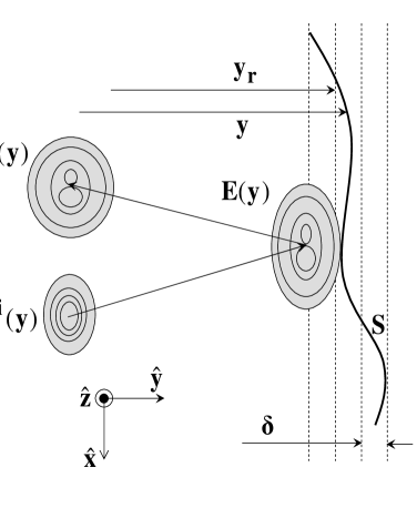
Figure 3: Illustration of the FFT-based efficient algorithm for the phase gradient method. ${\bf E}^{i}$ and ${\bf E}^{r}$ are the incident electric field and reflected electric field respectively. $S$ is the PEC mirror phase corrector. $y$ is the coordinate of the PEC mirror phase corrector and $y_{r}$ is the coordinate of the slicing reference plane. $\delta$ is the spacing between two adjacent slicing reference planes.

V. An Efficient Algorithm for Phase Gradient Method

By slicing the PEC mirror phase corrector into many subdomains, as shown in Fig. 3, the FFT can be used [3, 6] to compute the electric field ${\bf E}$ and it’s derivatives,

$${\bf E}(y)=\hbox{IFT}\left\{\begin{array}[]{cc}\\ \\ \end{array}{\bf F}(k_{x},k_{z})e^{-ik_{y}y}\begin{array}[]{cc}\\ \\ \end{array}\right\},\ \ \ {\bf F}(k_{x},k_{z})=\hbox{FT}\left\{\begin{array}[]{cc}\\ \\ \end{array}{\bf E}(y=0)\begin{array}[]{cc}\\ \\ \end{array}\right\}$$ (38)

$$\frac{\partial{\bf E}(y)}{\partial v}=\hbox{IFT}\left\{\begin{array}[]{cc}\\ \\ \end{array}-ik_{v}{\bf F}(k_{x},k_{z})e^{-ik_{y}y}\begin{array}[]{cc}\\ \\ \end{array}\right\},\ \ \ \ \ v=x,z$$ (43)

where, the Fourier Transform (FT) and the Inverse Fourier Transform (IFT) are defined as follows,

$$\hbox{FT}\left\{\begin{array}[]{cc}\\ \end{array}\cdot\begin{array}[]{cc}\\ \end{array}\right\} \equiv \frac{1}{2\pi}\int_{-\infty}^{\infty}dxe^{ik_{x}x}\int_{-\infty}^{\infty}\left\{\begin{array}[]{cc}\\ \end{array}\cdot\begin{array}[]{cc}\\ \end{array}\right\}e^{ik_{z}z}dz$$ (48)

$$\hbox{IFT}\left\{\begin{array}[]{cc}\\ \end{array}\cdot\begin{array}[]{cc}\\ \end{array}\right\} \equiv \frac{1}{2\pi}\int_{-\infty}^{\infty}dk_{x}e^{-ik_{x}x}\int_{-\infty}^{\infty}\left\{\begin{array}[]{cc}\\ \end{array}\cdot\begin{array}[]{cc}\\ \end{array}\right\}e^{-ik_{z}z}dk_{z}$$ (53)

The wrapped phase difference $\delta\check{\theta}=\left(\check{\theta}^{i}-\check{\theta}^{r}\right)$ is obtained from (38). Due to similarity, only x-component $\hat{\bf x}\hbox{E}_{x}$ is considered here,

$$\delta\check{\theta}_{x}=\arctan\left[\frac{\Im\left(\begin{array}[]{cc}\\ \\ \end{array}\hbox{IFT}\left\{\hbox{ F}^{r}_{x}(k_{x},k_{z})e^{-ik_{y}y}\right\}\begin{array}[]{cc}\\ \\ \end{array}\right)}{\Re\left(\begin{array}[]{cc}\\ \\ \end{array}\hbox{IFT}\left\{\hbox{ F}^{r}_{x}(k_{x},k_{z})e^{-ik_{y}y}\right\}\begin{array}[]{cc}\\ \\ \end{array}\right)}\right]-\arctan\left[\frac{\Im\left(\begin{array}[]{cc}\\ \\ \end{array}\hbox{IFT}\left\{\hbox{ F}^{i}_{x}(k_{x},k_{z})e^{-ik_{y}y}\right\}\begin{array}[]{cc}\\ \\ \end{array}\right)}{\Re\left(\begin{array}[]{cc}\\ \\ \end{array}\hbox{IFT}\left\{\hbox{ F}^{i}_{x}(k_{x},k_{z})e^{-ik_{y}y}\right\}\begin{array}[]{cc}\\ \\ \end{array}\right)}\right]$$ (70)

With the help of (38)-(53), the gradient of the phase difference $\nabla\left(\delta\theta_{x}\right)$ on the slicing reference plane $y_{r}$ in Fig. 3 can be obtained from (29),

$$\nabla\left(\delta\theta_{x}\right)=\nabla\left(\delta\check{\theta}_{x}\right)=\Re\left[\frac{\hbox{IFT}\left\{{\bf k}\hbox{ F}^{i}_{x}(k_{x},k_{z})e^{-ik_{y}y}\right\}}{\hbox{IFT}\left\{\hbox{ F}^{i}_{x}(k_{x},k_{z})e^{-ik_{y}y}\right\}}-\frac{\hbox{IFT}\left\{{\bf k}\hbox{ F}^{r}_{x}(k_{x},k_{z})e^{-ik_{y}y}\right\}}{\hbox{IFT}\left\{\hbox{ F}^{r}_{x}(k_{x},k_{z})e^{-ik_{y}y}\right\}}\right]$$ (71)

To obtain the PEC mirror surface correction $\delta_{\hat{\bf y}}$ through (13), $\delta\check{\theta}_{x}$ has to be unwrapped. Here, an FFT-based phase unwrapping algorithm is presented for the $r$-norm minimum problem given in (9). Suppose that $\delta\theta_{x}$ can be expressed in the Fourier series,

$$\delta\theta_{x}=\hbox{IFT}\{f(k_{x},k_{z})\}$$ (72)

Then,

$$\frac{\partial\left(\delta\theta_{x}\right)}{\partial v}=\hbox{IFT}\{-ik_{v}f(k_{x},k_{z})\},\ \ \ \ \ v=x,z$$ (73)

To obtain $\delta\theta_{x}$, the Fourier coefficient $f(k_{x},k_{z})$ is chosen to minimize the cost function $Q$ given in (9), with $w_{x}=w_{z}=1$. For LMS method where $r=2$, it can be shown that $f(k_{x},k_{z})$ takes the following form,

$$\frac{Q\left(f+\delta f\right)-Q\left(f\right)}{\delta f}=0\rightarrow f(k_{x},k_{z})=i\frac{k_{x}\hbox{FT}\left\{\nabla\left(\delta\check{\theta}_{x}\right)\cdot\hat{\bf x}\right\}+k_{z}\hbox{FT}\left\{\nabla\left(\delta\check{\theta}_{x}\right)\cdot\hat{\bf z}\right\}}{k_{x}^{2}+k_{z}^{2}}$$ (74)

Now, the PEC mirror surface correction $\delta_{\hat{\bf y}}$ can be obtained from (13), with the help of (71)-(74).

VI. Discussion

It has been shown that both the GO method and the phase gradient method can be used in the PEC mirror phase corrector design. Both methods have their advantages and disadvantages, e.g., the GO method is simple and easy to use, but it is time-consuming; the phase gradient method is efficient (due to the use of FFT), but it’s application is limited by the sampling theorem. In general, the GO method is suitable for problems of significant side lobes; and the phase gradient method is suitable for problems of smooth phase front with negligible side lobes.

VII. Conclusion

In this article, both the GO method and the phase gradient method have been presented for the PEC mirror phase corrector design. The FFT-based efficient algorithm has been proposed for the phase gradient method to speed up the design procedure.

Acknowledgements

This work was supported by the U.S. Dept. of Energy under the contract DE-FG02-85ER52122.

Bibliography

- [1] R. Cao and R. J. Vernon, “Improved performance of three-mirror beam-shaping systems and application to step-tunable converters,” the 30 Int. Conf. on Infrared and Millimeter Waves, Williamsburg, Virginia, USA, Sep. 19-23, 2005, pp. 616-617.
- [2] Michael P. Perkins and R. J. Vernon, “Iterative design of a cylinder-based beam-shaping mirror pair for use in a gyrotron internal quasi-optical mode converter,” the 29 Int. Conf. on Infrared and Millimeter Waves, Karlsruhe, Germany, Sep. 27-Oct. 1, 2004.
- [3] S.-L. Liao and R. J. Vernon, “A new fast algorithm for field propagation between arbitrary smooth surfaces”, the joint 30 Infrared and Millimeter Waves and 13 International Conference on Terahertz Electronics, Williamsburg, Virginia, USA, 2005, ISBN: 0-7803-9348-1, INSPEC number: 8788764, DOI: 10.1109/ICIMW.2005.1572687, Vol. 2, pp. 606-607.
- [4] S.-L. Liao and R. J. Vernon, “The near-field and far-field properties of the cylindrical modal expansions with application in the image theorem,” the 31 Int. Conf. on Infrared and Millimeter Waves, Shanghai, China, IEEE MTT, Catalog Number: 06EX1385C, ISBN: 1-4244-0400-2, Sep. 18-22, 2006.
- [5] S.-L. Liao and R. J. Vernon, “The cylindrical Taylor-interpolation FFT algorithm,” the 31 Int. Conf. on Infrared and Millimeter Waves, Shanghai, China, IEEE MTT, Catalog Number: 06EX1385C, ISBN: 1-4244-0400-2, Sep. 18-22, 2006.
- [6] S.-L. Liao and R. J. Vernon, “Sub-THz beam-shaping mirror designs for quasi-optical mode converter in high-power gyrotrons”, J. Electromagn. Waves and Appl., scheduled for volume 21, number 4, page 425-439, 2007.
- [7] Shaolin Liao and R.J. Vernon, “A new fast algorithm for calculating near-field propagation between arbitrary smooth surfaces,” In 2005 Joint 30th International Conference on Infrared and Millimeter Waves and 13th International Conference on Terahertz Electronics, volume 2, pages 606-607 vol. 2, September 2005. ISSN: 2162-2035.
- [8] Shaolin Liao, Henry Soekmadji, and Ronald J. Vernon, “On Fast Computation of Electromagnetic Wave Propagation through FFT,” In 2006 7th International Symposium on Antennas Propagation EM Theory, pages 1-4, October 2006.
- [9] Shaolin Liao, “Beam-shaping PEC Mirror Phase Corrector Design,” PIERS Online, 3(4):392-396, 2007.
- [10] Shaolin Liao, “Fast Computation of Electromagnetic Wave Propagation and Scattering for Quasi-cylindrical Geometry,” PIERS Online, 3(1):96-100, 2007.
- [11] Shaolin Liao, “On the validity of physical optics for narrow-band beam scattering and diffraction from the open cylindrical surface,” Progress in Electromagnetics Research Symposium (PIERS), vol. 3, no. 2, pp. 158–162 Mar., 2007. arXiv:physics/3252668. DOI: 10.2529/PIERS060906142312
- [12] Shaolin Liao, Ronald J. Vernon, and Jeffrey Neilson, “A high-efficiency four-frequency mode converter design with small output angle variation for a step-tunable gyrotron,” In 2008 33rd International Conference on Infrared, Millimeter and Terahertz Waves, pages 1-2, September 2008. ISSN: 2162-2035.
- [13] S. Liao, R. J. Vernon, and J. Neilson, “A four-frequency mode converter with small output angle variation for a step-tunable gyrotron,” In Electron Cyclotron Emission and Electron Cyclotron Resonance Heating (EC-15), pages 477-482. WORLD SCIENTIFIC, April 2009.
- [14] Ronald J. Vernon, “High-Power Microwave Transmission and Mode Conversion Program,” Technical Report DOEUW52122, Univ. of Wisconsin, Madison, WI (United States), August 2015.
- [15] Shaolin Liao, Multi-frequency beam-shaping mirror system design for high-power gyrotrons: theory, algorithms and methods, Ph.D. Thesis, University of Wisconsin at Madison, USA, 2008. AAI3314260 ISBN-13: 9780549633167.
- [16] Shaolin Liao and Ronald J. Vernon, “A Fast Algorithm for Wave Propagation from a Plane or a Cylindrical Surface,” International Journal of Infrared and Millimeter Waves, 28(6):479-490, June 2007.
- [17] Shaolin Liao, “Miter Bend Mirror Design for Corrugated Waveguides,” Progress In Electromagnetics Research, 10:157-162, 2009.
- [18] Shaolin Liao and Ronald J. Vernon, “A Fast Algorithm for Computation of Electromagnetic Wave Propagation in Half-Space,” IEEE Transactions on Antennas and Propagation, 57(7):2068-2075, July 2009.
- [19] Shaolin Liao, N. Gopalsami, A. Venugopal, A. Heifetz, and A. C. Raptis, “An efficient iterative algorithm for computation of scattering from dielectric objects,” Optics Express, 19(4):3304-3315, February 2011. Publisher: Optical Society of America.
- [20] Shaolin Liao, “Spectral-domain MOM for Planar Meta-materials of Arbitrary Aperture Wave-guide Array,” In 2019 IEEE MTT-S International Conference on Numerical Electromagnetic and Multiphysics Modeling and Optimization (NEMO), pages 1-4, May 2019.
- [21] R. Gerchberg and W. Saxton, “A practical algorithm for the determination of phase from image and diffraction plane pictures, ” Optik, Vol. 35, No. 2, 1972, pp. 237-246.
- [22] D. Ghiglia and M. Pritt, Two-Dimensional Phase Unwrapping Theory, Algorithms, and Software, John Wiley & Sons, New York, 1998.