Cerman: Software for simulating streamer propagation in dielectric liquids based on
the Townsend–Meek criterion

Abstract

We present a software to simulate the propagation of positive streamers in dielectric liquids. Such liquids are commonly used for electric insulation of high-power equipment. We simulate electrical breakdown in a needle–plane geometry, where the needle and the extremities of the streamer are modeled by hyperboloids, which are used to calculate the electric field in the liquid. If the field is sufficiently high, electrons released from anions in the liquid can turn into electron avalanches, and the streamer propagates if an avalanche meets the Townsend–Meek criterion. The software is written entirely in Python and released under an MIT license. We also present a set of model simulations demonstrating the capability and versatility of the software.

1 Introduction

1.1 Streamers in liquids

Dielectric liquids, specifically transformer oils, are used as electric insulation in high-power equipment such as power transformers [1]. Equipment failure is always a possibility, and in a world with ever-growing need for energy, there is a continuous effort to make equipment better, cheaper, more compact, and more environmentally friendly. To prevent equipment failure due to electrical discharges, new insulating liquids as well as additives are tested, experiments are carried out to better understand the physical nature of the phenomena, and simulations are performed to test the validity of predictive models [2, 3].

Since electrical discharge events are rare at operating conditions, model experiments are designed to induce discharge in the liquid. In one such model experiment, a needle electrode is placed opposing a planar electrode, where the needle–plane gap is insulated by a liquid [2]. If high voltage is applied, resulting in a sufficiently strong electric field close to the needle, the liquid will lose its insulating properties and begin to conduct electricity, and subsequent (partial) discharges from the needle into the liquid can occur. The charge transported into the liquid can increase the electric field and lead to partial discharges in new regions in a self-induced manner. Shadowgraphic images (an imaging technique exploiting differences in permittivity) reveal that a gaseous channel, a “streamer”, is formed and how it branches as it propagates through the liquid [4]. If a streamer bridges the gap between two electrodes, an electric discharge can follow, possibly destroying the affected equipment.

Streamers are commonly classified by their polarity and speed of propagation from the slow 1st mode to the fast 4th mode, ranging from below $0.1\text{\,}\mathrm{k}\mathrm{m}\mathrm{/}\mathrm{s}$ to well above $100\text{\,}\mathrm{k}\mathrm{m}\mathrm{/}\mathrm{s}$ [2]. Streamers with negative polarity typically have a lower inception voltage than streamers with positive polarity (positive streamers), however, positive streamers typically lead to breakdowns at lower voltage than negative streamers, and as such, research is mainly concerned with positive streamers. The streamer phenomenon involves processes covering several length and time scales. Speed and branching is studied in gaps of different sizes ($\mathrm{m}\mathrm{m}$–$\mathrm{m}$), while many of the interesting processes, such as field ionization, high-field conduction, electro-hydrodynamic movement, bubble nucleation, cavitation, electron avalanches, photoionization, occur on a $\mathrm{\SIUnitSymbolMicro m}\text{/}$-scale [2, 3]. A streamer usually stops or leads to a breakdown on a $\mathrm{\SIUnitSymbolMicro s}\text{/}$-scale ($$\mathrm{k}\mathrm{m}\mathrm{/}\mathrm{s}$=$\mathrm{m}\mathrm{m}\mathrm{/}\mathrm{\SIUnitSymbolMicro}\mathrm{s}$$), whereas processes such as recombination of electrons and anions can occur within picoseconds. Consequently, experimentation as well as simulation is challenging.

1.2 Modeling and simulations

While sophisticated equipment is required for experiments, simulations often investigate the effect of given processes through relatively simple models. The fractal nature of the streamer structure can be simulated by considering a lattice where each point is either part of an electrode, the liquid, or the streamer [5]. Here, the streamer expands to new lattice points when some criterion, such as electric field strength, is obtained. Through kinetic Monte Carlo methods, the stochastic nature and the physical time can also be studied in such simulations [6]. By considering the streamer as an electrical network of resistors and capacitors, the charge and conduction can be studied, without necessarily confining the points of the network to a grid [7]. Models where the streamer consists of a set of discrete points are simplistic but also efficient. Conversely, with a higher demand for computational power, computational fluid dynamic (CFD) methods can be applied to solve the equations for generation and transport of charged particles (the flow of natural particles is often ignored) during a streamer discharge [8, 9], while the stochasticity and branching of streamers can be introduced by adding impurities [10]. Such CFD-calculations often ignore the phase change from liquid to gas as well and are confined to a small region because of the computational complexity. However, for simplified, single-channel streamers, both the phase change and the processes in the channel can be simulated [11, 12]. Code used for simulation of streamers in liquids is rarely published, in fact, we found just a single example [13].

1.3 Avalanche model

Figure 1: Illustration of the main components in the simulation model. The needle electrode and the streamer heads are hyperboloids, each with a potential $V_{i}$. A region of interest (ROI) is used to limit the computational effort to a region surrounding the active part of streamer. The ROI controls the position of the “seeds”, which are classified as anions, electrons, or avalanches, depending on the electric field strength at their position. The “shadowgraphic” image of the streamer is created by plotting all former positions of streamer heads.

We have previously described our streamer model for positive streamers where the propagation is based on an electron avalanche mechanism [14]. The model has been extended to account for conductance in the streamer channel and capacitance between the streamer and the planar electrode [15], as well as photoionization in front of the streamer [16], the latter as a mechanism for the transition from slow to fast propagation.

Streamer propagation is simulated in a setup resembling model experiments, a needle–plane gap filled with a model liquid, see figure 1 for details. The needle and streamer give rise to an electric field, affecting charged particles in the liquid. A number of anions, “seeds” for electron avalanches, is modeled within a volume surrounding the streamer, a “region of interest” (ROI). Electrons released from the anions can create electron avalanches, and the streamer propagates when an avalanche meets the Townsend–Meek criterion, i.e. exceeds a critical number of electrons [14]. The needle and the streamer heads (the extremities of the streamer) are modeled as hyperboloids, which simplifies calculating the electrical field since the Laplacian is analytic in prolate spheroid coordinates [17]. The electric field and potential is calculated by considering electrostatic shielding [14], as well as the conductance in the channel and the capacitance towards the planar electrode [15]. The streamer undergoes a transition into a fast propagation mode when radiation from the streamer head can ionize molecules directly in front of the streamer [16]. More details on the model is given in section 3.

The main output of the simulations include the propagation speed, the streamer shape (branching), and propagation distance. In addition, properties such as the initiation time, the potential of individual streamer heads, electric breakdown within the streamer channel, and avalanche growth, can also be investigated. Simulations show how various parameters affect the results, where the gap size, applied voltage, and type of liquid are important parameters for a simulation. Furthermore, other parameters such as the size of a streamer head, the conductivity of the streamer channel, properties of additives, and avalanche growth parameters can be varied to validate whether the underlying physical models are reasonable.

1.4 Scope

The present work describes the use, functionality and implementation of Cerman [18], a software to do simulations with our model [14, 15, 16], with the purpose to make the software publicly available. Section 2 demonstrates how to set up, simulate, and evaluate results of a relevant problem. Further details on the model and its implementation are given in section 3, whereas section 4 outlines the current functionality and some prospects for the future. A summary is then given in section 5. Furthermore, details on the algorithm is included in A, simulation parameters in B, and simulation example input files in C.

2 Simulation – using the software

Listing 1: Example of JSON-input file, gtcmsim.json, defining a simulation series with several values for the needle voltage $V_{0}$ and the threshold for breakdown in the streamer channel $E_{\textrm{bd}}$, both with and without photoionization enabled. Furthermore, each permutation is to be carried out 10 times with different initial seed positions. Note, by setting gtalphakind to gtA1991, $\alpha$ is calculated by 5. See B for a description of the parameters.

⬇

{

"gap_size": 0.010,

"needle_radius": 6e-06,

"needle_voltage": "linspace(60e3, 150e3, 10)",

"liquid_name": "cyclohexane",

"alphakind": "A1991",

"liquid_Ealpha": 0.65e09,

"liquid_IP": 9,

"streamer_head_radius": 3e-06,

"streamer_U_grad": 0e+06,

"streamer_d_merge": 12.5e-6,

"streamer_scale_tvl": 0.1,

"streamer_photo_enabled": [false, true],

"streamer_photo_efield": 3.1e9,

"streamer_photo_speed": 20e3,

"rc_tau0": 1e-6,

"rc_breakdown": [0e6, 4e6, 8e6, 16e6, 64e6],

"random_seed": 1,

"simulation_runs": 10,

"save_specs_enabled": {

"stat": true,

"gp5": true

}

}

2.1 Software overview

The software name Cerman is an abbreviation of ceraunomancy, which means to control lightning or to use lightning to gain information. The implementation is done in Python, an open-source, interpreted, high-level, dynamic programming language [19], and the software is available on GitHub [18] under an MIT license. The software is script-based, and controlled through the command gtcerman, which is used for creation of input files, running simulations, and evaluating the results. When a simulation is started, the simulation parameters are loaded from an input file, and the classes for the various functions are initiated. See B for a summary of simulation parameters. The simulation itself is essentially a loop where seeds in the liquid are moved and the streamer structure is updated until the streamer stops or leads to a breakdown. The algorithm is detailed in A.

2.2 Getting started

Download Cerman from GitHub [18] and install it by running

⬇

pip install .

from the downloaded folder. This installs the python package and the script gtcerman. Python 3.6 or above is required, as well as the packages gtnumpy [20], gtscipy [21], gtmatplotlib, gtsimplejson, and gtstatsmodels. The dependencies are automatically installed by gtpip. The software has been developed in OSX and has been tested on Linux as well.

2.3 Create simulation input

Figure 2: Visualization of the difference in parameter values between a selection of input files.

Each simulation requires a JSON-formatted input file where the parameters are given. Such files can be created from a master input file, specifying the parameters for a simulation series. A master input file can be created from a regular input file by changing a parameter value into a list of values. More than one parameter can contain lists, and all possible combinations of values is found to create the input files for the simulation series. To demonstrate, we use gtcmsim.json in listing 1, which specifies a simulation series exploring the influence of various parameters. The ten values for the applied voltage are specified through a gtlinspace-command, while the values for the threshold for breakdown in the channel and photoionization (fast mode) enabled are given in list form. Furthermore, gtsimulation_runs specifies the number of similar simulations, only differing by gtrandom_seed. If gtrandom_seed is gtnull, then each input file is created with a random number as gtrandom_seed, and when a number is specified, a range of number is generated, in this case, the numbers 1 through 10. Note that gtrandom_seed refers to the seed number for initializing the random number generator, not to the seeds within the ROI. However, a given gtrandom_seed does corresponds to a given initial positions of the seed anions. Defining fixed a gtrandom_seed for each simulation series makes it easier to see how a change in a given value affects the simulation, but for analyzing a larger assemble of simulations, it is usually preferable that the simulations are uncorrelated, i.e. have random initial anion placement.

Individual input files are created by running the gtcerman with the argument gtci (create input) and specifying which file to expand with gt-f:

⬇

cerman ci -f <filename>

This command creates a a number of new files by permutation of all lists in the given input file. The permutation of 10 random seeds, 10 applied voltages, 5 breakdown thresholds, and 2 modes for photoionization in listing 1 results in 1000 files. By default, the random seed is expanded first, followed by the needle voltage, which is is useful to consider when designing a simulation series. Choosing an appropriate number of values for these two parameters makes it easier to search for simulation files with given properties. When expanding the example in listing 1, the least significant digit gt??X indicates random seed number, the second digit gt?X? indicates the needle voltage, while the most significant digit gtX?? indicates the threshold for breakdown in the streamer channel and whether photoionization is enabled or not.

The action gtpp (plot parameters) creates a matrix representation of the parameter variation in set of input files, and is used like

⬇

cerman pp -g <pattern>

The argument gt-g specifies the pattern to search (or “glob”) for, e.g. gtcmsim_?00.json. The files are plotted at the $x$-axis and the varied parameters on the $y$-axis, see figure 2 for an example output. The name of the output file is based on the first file in the pattern.

After ensuring that the input parameter values are as desired, simulations are run using

⬇

cerman sims -g <pattern> -m <no>

which creates a queue of all files matching the pattern, and simulates a given number in parallel. For instance, gtcerman sims -g "cmsim_?5?.json" -m 15, simulates all input files with the same voltage, creating a queue where up to 15 separate subprocesses each run one simulation. These python processes are single threaded, and works best if gtnumpy is limited to a single thread as well. Each simulation dumps the input parameters and progress information to a log file. For each simulation we then have a parameter file, a log file, and one or more save files. The files are named by extending the name of the master file, e.g.

⬇

cmsim.json # master file

cmsim_290.json # input parameters

cmsim_290.log # log file

cmsim_290_gp5.pkl # save file

cmsim_290_stat.pkl # save file

2.4 Evaluate results

The results are evaluated by parsing the data stored from one or more simulations. The input file, listing 1, defines two “save specifications” as gttrue, i.e. enabled, each defining various simulation data to be dumped to disk at given intervals or occasions. The gtsave_spec called gtstat saves iteration number, CPU time, simulation time, leading head $z$ position, number of critical avalanches, and the position of each new streamer head, for every iteration. This enables evaluation of the shape of the streamer and its propagation speed. The gtsave_spec called gtgp5 saves most of the data available, including the position of all the seeds (anions/electrons/avalanches), for every 5 percent of streamer propagation, i.e. a total of 20 times for a breakdown streamer. The data is saved using gtpickle and can be loaded to analyze a given iteration, a whole simulation, or by combining data from several simulation.

Evaluate iterations. Iteration data can be used to analyze the details of a simulation. This is particularly useful when evaluating the validity of the simulation parameters. Use for instance

⬇

cerman pi seedheads -r <start stop> -g <pattern>

where gtpi means “plot iteration” and gtseedheads is a scatter plot of avalanches and the streamer head configuration. The option gt-r controls the range of iterations to plot. Figure 28 in [14] shows a number of such plots.

Figure 3: (left) Streak plots where “options” have been used to limit the $x$-axis and to show $V$, $E_{\textrm{bd}}$, and photoionization on the legend. (right) Shadow plots where each streamer is plotted with an offset and the legend is hidden. The legend is the same for both plots.

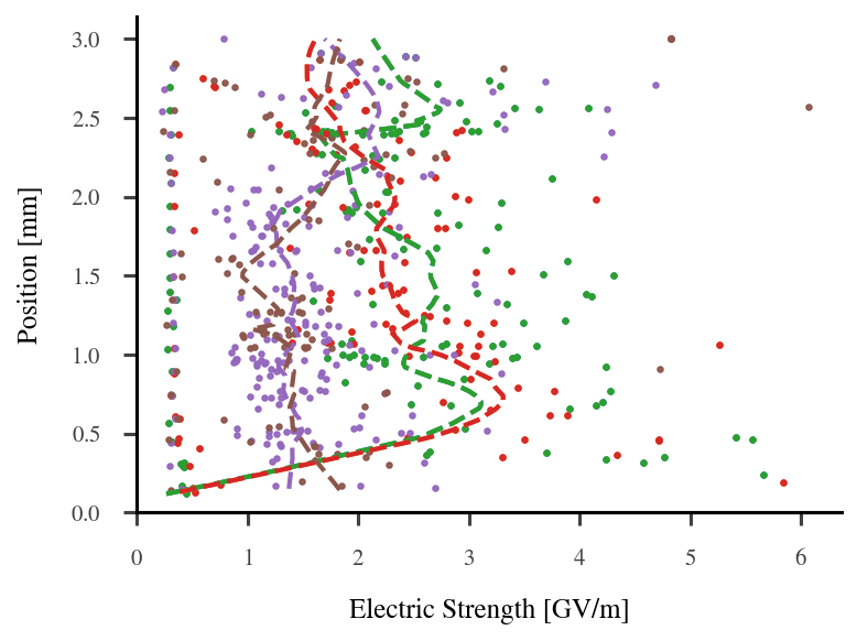
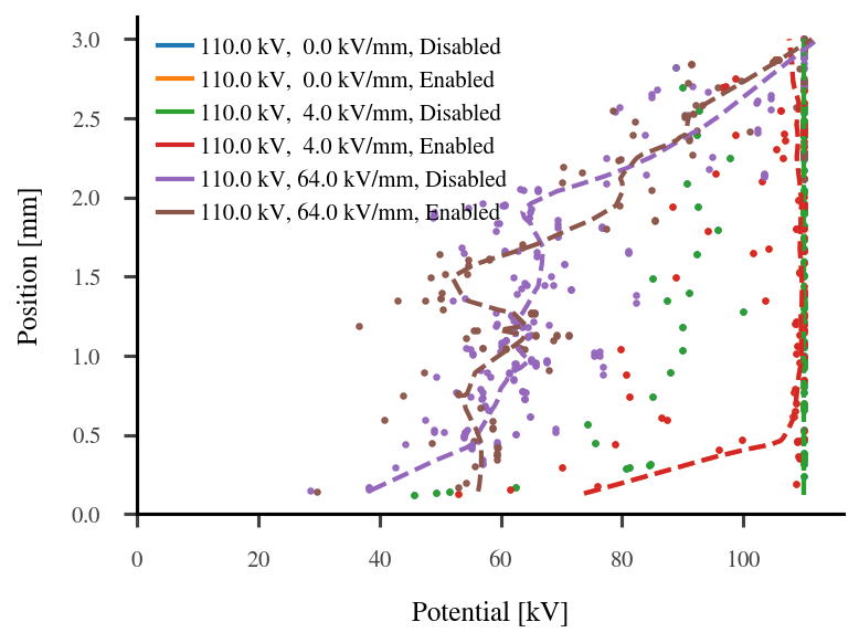
Figure 4: The electric strength (left) and the electric potential (right) at the tip of each new streamer head. The streamer heads are sampled for every 5 % of propagation. The “options” are used to control which streamer heads to use for the calculation and which positions to calculate for.

Evaluate simulations. Use gtps for simulation plots. These are mainly plotted with the $z$-position in the gap on the $y$-axis. Plotting the $x$- or $y$-position of streamer heads on the $x$-axis, using gtshadow, gives a “shadowgraphic” plot of the streamer:

⬇

cerman ps shadow -g <pattern> -o <options>

Similarly, plotting the propagation time on the $x$-axis is done in a gtstreak plot. Options can be added to control the limits/extents of the plot, the figure size, the behavior of the legend, redefining the axis labels, starting each plot with an offset, saving the plotted data to a JSON-file, and much more. Use gthelp to show available commands and options, for instance:

⬇

cerman help # for the main script

cerman ps help # for plot simulation

cerman ps shadow -o help # for shadow plot

Single simulation data may be of interest, but it is often better to compare several simulations in the same plot to visualize how the input parameters affect the results. The gtgp5 save requires a lot of disk space, but can be very useful in analyzing the data. For plotting the potential of each head, use

⬇

cerman ps headsestr -g <pattern> -o <options>

The current (active) heads of the streamer is selected, their potential is scaled (electrostatic shielding, using a nnls-approach, cf. [14]), and then, the electric field at their position is calculated. However, the options can be used to specify the method for scaling and which positions to calculate the field for, e.g. at the position of each appended (new) streamer head. The electric field strength and electric potential are presented as scatter plots against the $z$-position of each given position, as well as dashed line indicating the average value, see figure 4.

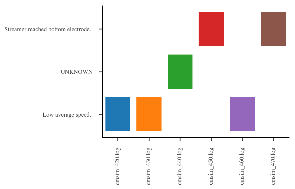
Figure 5: Example, parsing the log files to visualize how simulations have terminated. “Unknown” implies that the simulation is not complete (ongoing or aborted).

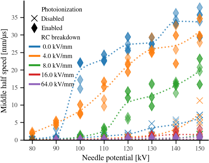
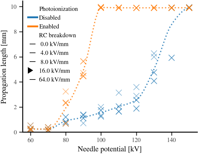
Figure 6: Example, combination plots: (left) propagation speed using both markers and colors, and (right) propagation length for only a given value of one parameter with the other parameter colored.

Evaluate a series of simulations. The difference in the simulated parameters can be visualized using gtpp and globbing for the gtpkl-files or gtlog-files. An existing gtlog-file indicates that a simulation was initiated. The command

⬇

cerman psr -g <pattern>

parses log files and plots the reasons why the simulations were terminated. An example of such a plot is shown in figure 5. This is a good way to verify that simulations have completed successfully.

When all simulations are completed and verified, parse all the save files and build a combined database of the results:

⬇

cerman ca -g <pattern> -o mode=reload

The option gtreload forces files to be parsed, even if they already are in the database. When parsing the save files, a number of properties are extracted or calculated. Results such as propagation length (ls), average propagation speed (psa), inception time (ita), average jump distance (jda), simulation time (st), and computational time (ct) are saved in the database. The results are plotted by using

⬇

cerman pr <parameter> -f <file> -o <options>

The parameter gives the $x$-axis of the plot, for instance gtv (needle voltage). The results to plot is given through the option, e.g. gt-o ykeys=ls_psa. The software inspects the database of parsed save files for varied parameters and automatically create plots of all possible permutations using colors and markers. Figure 6 shows a selection of such plots, where needle voltage is on the $x$-axis and the other parameters have been added automatically.

As illustrated, the software has been designed to facilitate simulating and analyzing a large simulations series in a semi-automatic fashion. The individual simulations have their parameters defined in dedicated files, while the behavior of the gtcerman-script is defined by command line arguments.

3 Model implementation

This section describes the implementation of our model [14, 15, 16] in more detail. An overview of the model is already given in section 1.3, and figure 1 is useful for understanding the principal setup, a needle–plane gap where electron avalanches grow from single electron seeds.

The electric field. The needle electrode and the streamer heads are modeled as hyperboloids. The Laplacian electric potential $V_{i}$ and electric field $\bm{E}_{i}$ from a streamer head $i$ is calculated analytically in prolate spheroid coordinates [14]. For a position $\bm{r}$, the electric potential $V(\bm{r})$ and field $\bm{E}(\bm{r})$ is given by the superposition principle,

$$V(\bm{r})=\sum_{i}k_{i}V_{i}(\bm{r})\quad\text{and}\quad\bm{E}(\bm{r})=\sum_{i}k_{i}\bm{E}_{i}(\bm{r})\,,$$ (1)

where the coefficients $k_{i}$ are introduced to account for electrostatic shielding. An optimization is performed such that the unshielded potential at the tip of any streamer head $j$ equals the sum of all the shielded potentials at that position, $V_{j}(\bm{r_{j}})=\sum k_{i}V_{i}(\bm{r_{j}})$ [14].

Region of interest (ROI). The ROI is a cylindrical volume used to control the position of seeds, see figure 1. Note, the seeds in this respect include all anions, electrons, and even all avalanches. The number of seeds in a simulation is given by the specified density of seeds and the volume of the ROI. Initially, the seeds are placed at random positions within the ROI. When a seed falls behind the ROI, collides with the streamer, or creates a critical avalanche, it is removed and replaced by a new seed. The new seed is placed with a $z$-position one ROI-height closer to the plane, at a random $xy$-position (at a radius less than the ROI radius). The ROI volume is defined by a distance from the $z$-axis, and a given length above and below the leading streamer head, which is the part of the streamer closest to the planar electrode. When a new streamer head is created closer to the plane, the streamer propagates, and the ROI moves as well.

Anions, electrons, and electron avalanches. The electric field $E$ is calculated for each seed and the seeds are classified as avalanches ($E\geq E_{\textrm{c}}$), electrons ($E\geq E_{\textrm{d}}$), or anions ($E<E_{\textrm{d}}$), where the avalanche threshold $E_{\textrm{c}}$ and detachment threshold $E_{\textrm{d}}$ are given as input parameters. Seeds move in the electric field with a speed dependent on their mobility $\mu$, which gives the distance the seed moves, $\Delta\bm{s}=\bm{E}\mu\Delta t$, for a time step $\Delta t$. The number of electrons $N_{\textrm{e}}$ in an electron avalanche, starting from a single electron, can be calculated by [14]

$$N_{\textrm{e}}=\exp\sum_{i}\Delta s_{i}\alpha_{i}=\exp\sum_{i}E_{i}\,\mu_{\textrm{e}}\,\alpha_{\textrm{m}}\,e^{-{E_{\alpha}}/{E_{i}}}\Delta t_{i}\,,$$ (2)

where $\alpha$ is the avalanche growth, $\mu_{\textrm{e}}$ is the electron mobility, $\Delta t$ is the time step, and $i$ is an iteration, whereas the avalanche growth parameters $\alpha_{\textrm{m}}$ and $E_{\alpha}$ have been obtained from experiments [14]. In practice, however, we only calculate and store the exponent in 2, $Q_{\textrm{e}}=\ln N_{\textrm{e}}$,

$$Q_{\textrm{e}}=\sum_{i}\Delta Q_{i}=\sum_{i}\Delta s_{i}\alpha_{i}\,,$$ (3)

for each electron avalanche. When a low-IP additive is present, $\alpha$ is modified by adding a factor [14]

$$\alpha_{i,\text{add}}=\alpha_{i}(1-x_{\textrm{add}}+x_{\textrm{add}}e^{k_{\alpha}(I_{\textrm{b}}-I_{\textrm{a}})})$$ (4)

which is dependent on the mole fraction of the additive $x_{\textrm{add}}$, and the difference in IP between the base liquid $I_{\textrm{b}}$ and the additive $I_{\textrm{a}}$ modified by a factor $k_{\alpha}$ as prescribed by [22]. This is the default setting for the software. Another model for $\alpha$ given in [23] is also implemented:

$$\alpha_{i,\text{mod}}=\frac{3eE_{\alpha}^{2}}{I_{\textrm{b}}E_{i}}e^{-\frac{E_{\alpha}}{E_{i}}}\,.$$ (5)

This method is applied in listing 1.

Expanding the streamer structure. According to the Townsend–Meek criterion [24], streamer breakdown occurs when an avalanche exceeds a critical number of electrons $N_{\textrm{c}}=\exp(Q_{\textrm{c}})$. When an avalanche obtains $Q_{\textrm{e}}>Q_{\textrm{c}}$, we place a new streamer head at its position [14]. The initial potential of a new streamer head is calculated by considering the capacitance and potential of the closest existing streamer heads [15]. If adding the new head implies removing another head (see the paragraph below), the potential changes slightly, mimicking transfer of charge. However, if both the new and the present head stays, they share the “charge”, which gives a moderate reduction in the potential of both heads.

Optimizing the streamer structure. There are three criteria for removing heads. A streamer head $i$ is removed if

$$\nu_{j}(\bm{r}_{i})<\nu_{j}(\bm{r}_{j})\quad\text{or}\quad k_{i}<k_{\textrm{c}}\quad\text{or}\quad\big{(}({\lvert\bm{r}_{i}-\bm{r}_{j}\rvert}<d_{\textrm{m}})\text{ and }(z_{i}>z_{j})\big{)}\,,$$ (6)

are satisfied for any other streamer head $j$ [14]. The first condition checks whether the tip of one hyperbole ($\bm{r}_{i}$) is inside another hyperbole, a collision (the $\nu$-coordinate describes a hyperboloid, specifically the asymptotic angle). The second condition removes heads whose potential are to a high degree shielded by other heads (if the coefficient $k_{i}$ in 1 lower than a threshold $k_{c}$). The third condition checks whether two streamer heads are closer than $d_{\textrm{m}}$ and should be merged to a single head, where the one at the highest $z$-coordinate is removed.

Conduction and breakdown in the streamer channel. Conduction in the streamer channel increases the potential of each streamer head $i$ each iteration,

$$\Delta V_{i}=V_{0}-V_{i}\quad\rightarrow\quad V_{i}=V_{0}-\Delta V_{i}\,e^{-\Delta t/\tau_{i}}\,.$$ (7)

The time constant $\tau_{i}=RC\tau_{0}$ (for a given head $i$) is calculated from the resistance $R$ in the channel and the capacitance $C$ towards the plane [15]

$$R\propto\ell\,,\quad\text{and}\quad C\propto\left(\ln\frac{4z+2r_{\textrm{s}}}{r_{\textrm{s}}}\right)^{-1}\,,$$ (8)

where $\ell$ is the channel length (distance to the needle), $r_{\textrm{s}}$ is the tip curvature radius of the streamer head, and $z$ is the $z$-position of the streamer head. As such, each streamer head is treated as an individual RC-circuit, e.g. the three streamer heads in figure 1 would each have an individual resistance (channel) as well as an individual capacitance towards the planar electrode. If the conduction is low, the potential difference $\Delta V_{i}$ increases as the streamer propagates, and the electric field within the streamer channel $E_{\textrm{s}}=\Delta V_{i}/\ell_{i}$ may increase as well. If $E_{\textrm{s}}$ exceeds a threshold $E_{\textrm{b}}$, a breakdown occurs, equalizing the potential of the streamer head and the needle, which is achieved by setting $\tau_{i}=0$ in 7 for the given iteration.

Photoionization. Photoionization is a possible mechanism for fast streamer propagation [25]. We have proposed a mechanism in which the propagation speed of a streamer increases if the liquid cannot absorb radiation energy to excited states, as a result of a strong electric field reducing the ionization potential [16]. Since the full model, considering fluorescent radiation from the streamer head, and a field-dependent photoionization absorption cross section, is computationally expensive, a simpler model is used in the simulations. Instead we calculate the field strength $E_{w}$ required to reduce the ionization potential below the energy of the fluorescent radiation. In each iteration, if the electric field $E$ at the tip of a streamer head $i$ exceeds the parameter $E_{w}$, the head is moved a distance $\Delta\bm{s}_{i}$ towards the planar electrode,

$$\Delta\bm{s}_{i}=-v_{w}\,\Delta t\,\Theta\!\left(E(\bm{r}_{i})-E_{w}\right)\,\hat{\bm{z}}\,,$$ (9)

where $v_{w}$ is the photoionization speed, and $\Theta$ is the Heaviside step function. For more details on the entire model, see our previous work [14, 15, 16].

4 Current functionality and future prospects

The main function of the model and the software is to simulate streamers in a point–plane gap, using the Townsend–Meek criterion for propagation. The propagation criterion is met when electron avalanches obtain a given size. This model and the algorithm are fixed, but there are several parameters which can be adjusted. Changing experiment features such as needle tip radius, gap size, voltage, liquid properties, or the parameters of the algorithms, is straightforward. Proposals to extend the software to encompass new functionality is given in this section.

In [14] we explored the fundamental features off the model, i.e. a streamer consisting of charged hyperbolic streamer heads, and streamer growth by electron avalanches initiating from anions. The model predicts several aspects of streamer propagation, and shows how they are linked towards the values of given input parameters. The predicted propagation speed and the degree of branching were both lower than expected. We found how the speed was dependent mainly on the number of electron avalanches and their growth, while the branching was mainly related to how the streamer heads were configured and managed, which is mainly controlled by the parameters $k_{\textrm{c}}$ and $d_{\textrm{m}}$ in 6.

When new streamer heads were added, their potential was set assuming a constant electric field within the channel, resulting in a moderate voltage drop between the needle electrode and the streamer head [14]. To better represent the dynamics of the streamer channel, an RC-model was developed [15]. In the RC-model, the potential of new streamer heads is dependent of the potential of the closest existing streamer heads. If the conductance of the streamer channel is high, then the potential of the streamer head is kept close to that of the needle, giving results comparable to those without the RC-model. Conversely, having low conduction regulates the speed of the streamer, increasing the likelihood that more branches are able to propagate. Furthermore, the RC-model also allows for simulation of a breakdown within the streamer channel itself, which is likely what occurs during a re-illumination. This breakdown occurs when the electric field within the channel exceeds a given threshold.

The importance of photoionization during a streamer breakdown is unknown. We explored different aspects of photoionization in [16], and implemented a model for change to a fast propagating mode. Molecules excited by energetic processes, such as electron avalanches, can relax to a lower energy state by emitting radiation. We argued that fluorescent radiation can be important, and modeled how this radiation can cause ionization in high-field areas, since the high-field reduces the ionization potential.

In the current implementation, a square wave voltage is applied to the needle at the beginning of the simulation. It is easy to change the behavior to a voltage ramp, from zero to max over a given time. This can be the basis for a study on streamer inception where other parameters such as needle size and the electron properties of the liquid are investigated as well. Simulating a dynamic voltage, such as a lightning impulse, requires some more work, but is also achievable.

We have focused on cyclohexane since many of its properties are well known, but other non-polar insulating liquids can be studied by changing relevant parameters. The seed density $n_{\textrm{ion}}$ is based on the low-field conductivity $\sigma$ and electron mobility $\mu_{\textrm{e}}$ of the liquid, and the propagation speed scales linearly with both seed density $n_{\textrm{ion}}$ and electron mobility $\mu_{\textrm{e}}$. The electron avalanche growth parameters are also liquid-dependent, and $E_{\alpha}$ in particular has a big impact on the results [14]. Streamer parameters, such as conductivity of the streamer channel and streamer head radius, need to be reevaluated as well for other liquids. The properties of the streamer channel are also important to simulate the effects of external pressure, which mainly affects processes in the gaseous phase [26].

The effect of additives with a low ionization potential (IP) are modeled as causing an increase in electron avalanche growth [22, 14]. Other additives can easily be used as long as the IP of both the base liquid and the additive are known. Low-IP additives are known to facilitate the propagation of slow streamers and to increase the acceleration voltage, possibly as a result of increased branching [27], however the mechanisms involved are not known. It is possible that low-IP additives are sources of electrons that can initiate avalanches, produced for instance through photoionization or fluctuations in the electric field. Such mechanisms can be added to the model and simulated, but will require some work. Furthermore, the mechanisms of added electron scavengers can also be interesting for further investigation, and particularly if negative streamers are to be simulated [22].

Our primary concern have been with positive streamers, since these are more likely to lead to a complete breakdown than negative streamers. The model relies on electrons detaching from anions, moving towards regions where the field is higher, and then forming electron avalanches. The polarity of our model can easily be reversed, however, the electrons would then drift away and be unable to form avalanches. As such, a model for creation of new electrons is needed to simulate negative streamers with the software. Charge injection from the needle and the streamer can be one such mechanism [28]. Another option is to model electron generation (charge separation) in the high-field region surrounding the needle and the streamer. Such mechanisms are interesting for simulating positive streamers as well.

The hyperbole approximation simplifies the calculation of the electric field, both from the needle electrode and from the streamer heads. Other experimental geometries, such as plane–needle–plane, or even more realistic real-life geometries can be implemented. The challenge is to set the correct shielding or scaling of the streamer heads according to the influence of the geometry. Simpler geometric restrictions are easier to implement, for instance by manipulating the ROI. The streamer can be restricted to a tube by setting a low value for the maximum radius of the ROI. Another method is setting the “merge threshold” very high, such that the streamer is restricted to a single channel with a single head, which can be representative for a streamer in a tube [29].

There are many mechanisms that can be added to investigate different methods of streamer propagation, for instance effects of Joule heating or electro-hydrodynamic cavitation [30]. There are also several parts of the existing model that can be improved. Better calculation and balancing of charges and energy would greatly improve the model. For instance an electric network model where the streamer is consisting of several interconnected parts, in contrast to the current implementation where all the streamer heads are individually “connected” to the needle. Such an approach can give a better understanding of the charge flow in the different parts and branches of the streamer, as well as a better representation of the electric field. Development towards a model for a space-charge limited field [31] can further improve the electric field representation, however, possibly at a high computational cost.

5 Summary

We present a software for simulating the propagation of positive streamers in a needle–plane gap insulated by a dielectric liquid. The model is based on the Townsend–Meek criterion in which an electron avalanche have to obtain a given size for the streamer to propagate. The software was developed and used for simulating our models for electron avalanche growth [14], conductance and capacitance in the streamer channels [15], as well as photoionization in front of the streamer [16]. From the examples on how to set up, run, and evaluate simulations, others can recreate our previous results or create their own set of simulations. Furthermore, the overview of the implementation and algorithm serves as a good starting point for others to change or extend the functionality of the software.

Appendix A The algorithm

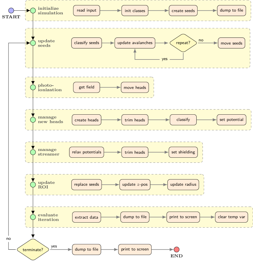
Figure 7: The simulation algorithm consists of initialization, a loop where the seeds and the streamer structure is updated, and then a finalization. It the loop, first the seeds (anions, electrons avalanches) are affected by the electric field, then the streamer structure is modified and this changes the electric field, finally the region of interest (ROI) is updated and the data from the iteration is evaluated. The loop concludes when one (of several) criterion is met, typically low propagation speed or reaching the opposing electrode. Details on each step is found in A.

This section describes the algorithm used to implement the model in more detail, essentially each part of figure 7, while referencing relevant parts from section 3.

Initialize simulation. The simulation input parameters are read and used to initialize classes for code profiling, simulation logging, calculation of avalanche growth, the needle, the streamer, the region of interest (ROI), the seeds (anions, electron, avalanches), how to save data, and how to evaluate simulation data. The initiation of the log file includes dumping the input parameters to the file. Given the ROI volume and the seed density, a number of seeds is created and placed within the ROI at random positions. Then, the save files are initialized by dumping the initial data, mainly information concerning the needle and the seeds.

Update seeds. The electric field $E$ is calculated for each seed (applying 1) and the seeds are classified as avalanches, electrons, and anions. All the avalanches move in the electric field and grow in size (see 2). The procedure is repeated until an avalanche collides with a streamer head, an avalanche meets the Townsend–Meek criterion, or a total of $N_{\textsc{msn}}$ repetitions has been performed. The “time” spent in this inner loop sets the time step for the current iteration of the main simulation loop. Finally, all the electrons and anions are moved. The inner loop over just the avalanches save significant computational time since the calculation of the electric field is the most expensive part of the computation and the avalanches is usually a small fraction of all the seeds.

Photoionization. The electric field at the tip of each streamer head is calculated and compared with the threshold for photoionization. Each streamer head where $E>E_{w}$ is “moved” a distance $v_{w}\Delta t$ towards $z=0$. Moving implies creating a new head, setting the potential by “transferring charge”, and removing the old head.

Manage new heads. For each critical avalanche a new head is created. If the simulation time step is set sufficiently low, there is usually zero or just one new head. The new head is discarded if it satisfies any of the criteria in 6, however, if adding it will cause another to be removed (later), the new head is classified as “merging”. If none of the criteria in 6 is met by adding the new head, i.e. all heads are kept, then it is a “branching” head, since adding it is potentially the start of a new branch. The potential of “merging” is set by “charge transfer” from the closest head, while “branching” heads have their potential set by “sharing charge” with the closest head, where the latter method also modifies the potential of the existing head [15].

Manage streamer. The potential of each streamer head is relaxed towards the potential of the needle by applying 7. This step increases the potential of the streamer head to the potential of the needle when a breakdown in the channel occurs. As mentioned above, the calculation of the electric field for the seeds is computationally expensive, and it actually scales with both the number of seeds and the number of streamer heads. It is therefore preferable to keep the number of heads to a minimum. Superfluous heads are trimmed according to the criteria in 6. Then, the electrostatic shielding is set for the trimmed structure.

Update ROI. Seeds that have moved behind the ROI, collided with the streamer, or lead to a critical avalanche are removed and replaced by a new seed. When a seed is replaced, the new seed is placed a distance, equal to the height of the ROI, closer to the plane, at a random $xy$-position within the ROI radius. If the streamer has moved closer to the plane, the ROI moves as well, and seeds behind the new position are replaced. If a streamer head is close to the edge of the ROI, the ROI expands towards the maximum radius. New seeds are created at random position within the expanded region.

Evaluate iteration. Iteration data is extracted from the various classes to be saved for later use. The data is used to evaluate whether any stop condition is fulfilled, and stored to dedicated classes. Which data to store and how often to sample the data is controlled by the user input. The saved data is dumped to a file at regular intervals to keep memory requirements of the program low. Information to monitor the progress is printed to the screen, at regular intervals. Finally, a number of temporary variables, relevant only to the iteration is cleared, and the program is prepared for a new iteration.

Terminate? If none of the conditions for stopping a simulation are met, the next iteration is performed. These conditions includes low streamer speed, streamer head close to the plane (breakdown), simulation time exceeded, computation time exceeded, and more. When a criterion is met, any unsaved data is dumped to disk, and a final logging to file and screen is performed, before the program terminates.

Appendix B Parameters

Table 1: Main parameters for simulation program. The experimental conditions specifies an overvoltage applied to medium size needle–plane gap. The values of the physical parameters in seeds and avalanches and streamer structure are justified in our previous work [14, 15, 16]. Parameter values related to the simulation algorithm, or the model in general, have also been discussed in previous work. See further description in B.

Property	Keyword	Symbol	Default
Experimental conditions
Distance from needle to plane	gap_size	$d_{\textrm{g}}$	$10\text{\,}\mathrm{mm}\text{/}$
Voltage applied to needle	needle_voltage	$V_{\textrm{n}}$	$100\text{\,}\mathrm{kV}\text{/}$
Needle tip radius	needle_radius	$r_{\textrm{n}}$	$6.0\text{\,}\mathrm{\SIUnitSymbolMicro m}\text{/}$
Seeds and avalanches
Seed number density	seeds_cn	$n_{\textrm{seeds}}$	$2\text{\times}{10}^{12}\text{\,}\mathrm{/}\mathrm{m}\mathrm{}{3}$
Anion mobility	liquid_mu_ion	$\mu_{\textrm{ion}}$	$0.30\text{\,}\mathrm{m}\mathrm{m}\mathrm{}{2}\mathrm{/}{\mathrm{V}\mathrm{s}}$
Electron mobility	liquid_mu_e	$\mu_{\textrm{e}}$	$45\text{\,}\mathrm{m}\mathrm{m}\mathrm{}{2}\mathrm{/}{\mathrm{V}\mathrm{s}}$
Liquid low-field conductivity	liquid_sigma	$\sigma_{\textrm{ion}}$	$0.20\text{\,}\mathrm{pS}\text{/}\mathrm{m}$
Electron detachment threshold	liquid_Ed_ion	$E_{\textrm{d}}$	$1.0\text{\,}\mathrm{MV}\text{/}\mathrm{m}$
Growth calculation method	alphakind	–	I2009
Critical avalanche threshold	Q_crit	$Q_{\textrm{c}}$	$23\text{\,}\text{/}$
Electron multiplication threshold	liquid_Ec_ava	$E_{\textrm{c}}$	$0.2\text{\,}\mathrm{GV}\text{/}\mathrm{m}$
Electron scattering constant	liquid_Ealpha	$E_{\alpha}$	$1.9\text{\,}\mathrm{GV}\text{/}\mathrm{m}$
Max avalanche growth	liquid_alphamax	$\alpha_{\textrm{m}}$	$130\text{\,}{\mathrm{\SIUnitSymbolMicro m}}^{-1}$
Additive IP diff. factor	liquid_k1	$k_{\alpha}$	$2.8\text{\,}\mathrm{eV}\mathrm{}{-1}$
Base liquid IP	liquid_IP	$I_{\textrm{b}}$	$10.2\text{\,}\mathrm{eV}\text{/}$
Additive IP	additive_IP	$I_{\textrm{a}}$	$7.1\text{\,}\mathrm{eV}\text{/}$
Additive mole fraction	additive_cn	$x_{\textrm{add}}$	$0.00\text{\,}\text{/}$
Streamer structure
Streamer head tip radius	streamer_head_radius	$r_{\textrm{s}}$	$6.0\text{\,}\mathrm{\SIUnitSymbolMicro m}\text{/}$
Minimum field in streamer channel	streamer_U_grad	$E_{\textrm{s}}$	$2.0\text{\,}\mathrm{kV}\text{/}\mathrm{mm}$
Streamer head merge distance	streamer_d_merge	$d_{\textrm{m}}$	$25\text{\,}\mathrm{\SIUnitSymbolMicro m}\text{/}$
Electrostatic shielding threshold	streamer_scale_tvl	$k_{\textrm{c}}$	$0.20\text{\,}\text{/}$
Photoionization threshold field	streamer_photo_efield	$E_{w}$	$3.1\text{\,}\mathrm{G}\mathrm{V}\mathrm{/}\mathrm{m}$
Photoionization added speed	streamer_photo_speed	$v_{w}$	$20\text{\,}\mathrm{k}\mathrm{m}\mathrm{/}\mathrm{s}$
Data type for field calculation	efield_dtype	–	float32
RC-model time constant	rc_tau0	$\tau_{0}$	$1\text{\,}\mathrm{\SIUnitSymbolMicro}\mathrm{s}$
RC resistance model	rc_resistance	–	linear
RC capacitance model	rc_capacitance	–	hyperbole
RC breakdown field	rc_breakdown	$E_{\textrm{bd}}$	$6\text{\,}\mathrm{k}\mathrm{V}\mathrm{/}\mathrm{m}\mathrm{m}$
Simulation algorithm
Time step of avalanche movement	time_step	$\Delta t$	$1.0\text{\,}\mathrm{ps}\text{/}$
Max avalanche steps per iteration	micro_step_no	$N_{\textsc{msn}}$	$100\text{\,}\text{/}$
Seed for random number generator	random_seed	–	None
Number of similar simulations	simulation_runs	–	10
ROI – behind leading head	roi_dz_above	$z^{+}_{\textsc{roi}}$	$1.0\text{\,}\mathrm{mm}\text{/}$
ROI – in front of leading head	roi_dz_below	$z^{-}_{\textsc{roi}}$	$1.0\text{\,}\mathrm{mm}\text{/}$
ROI – radius from center	roi_r_max	$r_{\textsc{roi}}$	$3.0\text{\,}\mathrm{mm}\text{/}$
Stop – low streamer speed	stop_speed_avg	$v_{\textrm{min}}$	$100\text{\,}\mathrm{m}\text{/}\mathrm{s}$
Stop – streamer close to plane	stop_z_min	$z_{\textrm{min}}$	$50\text{\,}\mathrm{\SIUnitSymbolMicro m}\text{/}$
Stop – avalanche time	stop_time_since_avalanche	$t^{\textrm{ava}}_{\textrm{max}}$	$100\text{\,}\mathrm{ns}\text{/}$
Sequential start number	seq_start_no	–	0
Enable profiling of code	profiler_enabled	–	False
Interval – dump save data to file	file_dump_interv	–	500
Interval – display data on screen	display_interv	–	500
Level of logging to file	log_level_file	–	20
Level of logging to console	log_level_console	–	20

The parameters for a simulation is supplied by the user in a JSON-formatted file (see listing 1). A list of all important parameters are shown in table 1. The potential, position and size of the needle are important parameters in an experiment and included in the first section, followed by parameters controlling the creation and movement of seeds (anions, electrons, and avalanches). The third section contains parameters related to the threshold for electron detachment, electron avalanche growth, and critical avalanche size. The parameters for the streamer can be split in two groups. The first group controls creation of the streamer heads and how the streamer heads are treated in relation to each other, whereas the second groups is related to the RC-model, controlling the potential of the streamer heads and the electric field in the streamer channel. There is also the option to choose whether the electric field from the streamer, acting on the seeds, is calculated using 32- or 64-bit precision. The latter requires about twice the time to compute. The parameters in the last section are mainly related to the simulation algorithm itself. The time step and the number of steps per loop are essential for a good results. The random seed, used to initialize the random number engine, controls the initial placement of seed anions. Choosing the same random number enables the study of, for instance, changing voltage with the same initial seed configuration. Conversely, not setting the random number makes the simulations uncorrelated, which is better for statistics. The size of the ROI decides how many seeds that are included in a simulation. For instance, an ROI of $10\text{\,}\mathrm{m}\mathrm{m}\mathrm{}\mathrm{3}$ in combination with a seed density of $2\text{\times}{10}^{12}\text{\,}\mathrm{/}\mathrm{m}\mathrm{}\mathrm{3}$ results in 20 000 seeds generated, a size which is easily treated by most computers. Finally, several parameters can be used to control how long a simulations will run, or to stop a simulation if the streamer stops or reaches the other electrode. There are also parameters controlling how often information is logged, and how detailed the logging should be.

Appendix C Example files

This appendix contains a number of examples of possible simulations. The files in listings 2, 3, 4 and 5 are all included in the folder gtexamples on GitHub [18].

Listing 2: The example file gtsmall_gap.json specifies a small gap and a range of voltages along with many parameter values equal to the defaults (cf. table 1). Although all values used in a simulation is stored in the log, it is nice to be explicit in the input as well. By specifying 10 gtsimulation_runs and 10 voltages, a total of 100 simulations is created from this file. Each simulation initiated with the seeds at uncorrelated positions since gtrandom_seed is gtnone.
Listing 3: The example file gtsmall_gap_mod.json builds on listing 2, but a number of parameters are modified, notably the seed density and the electron avalanche parameters, as well as several parameters for the streamer. All data is stored every 5th percent of propagation by gtgp5 and every 100th nanosecond by gtta07. Storing the properties of tens of thousands of seeds enables plotting of the development of seeds, but also requires a lot of disk space. Specifying gtstreamer saves all the streamer heads every 0.1 percent of propagation and is used to evaluate the development of the streamer. Since gtrandom_seed is 1 and gtsimulation_runs is 10, a range of gtrandom_seed from 1 through 10 is generated, giving the same 10 initial seed positions for each voltage.
Listing 4: The example file gtrc.json specifies the low and high conductivity within the streamer channel, and a range of threshold fields for electric breakdown in the streamer channel. The gtlinspace-command is a convenient method for creating a list of values. By combining 2 values for the conductivity and 5 values for breakdown with 10 values for the voltage, a total of 100 simulations are created from this file.
Listing 5: The example file gtpi.json specifies electrical breakdown in the streamer channel, with and without photoionization enabled, The keyword gtuser_comment does not affect the simulations, but can be convenient to set. 600 input files are created when expanding this file (100 voltages, with and without photoionization, for three different breakdown thresholds).

Listing 2: The example file gtsmall_gap.json specifies simulations similar to the baseline studies in section 3.1 in [14].

⬇

{ "gap_size": 0.003,

"needle_radius": 6e-06,

"needle_voltage": [30e3, 40e3, 50e3, 60e3, 70e3,

80e3, 90e3, 100e3, 110e3, 120e3],

"liquid_name": "cyclohexane",

"liquid_alphamax": 200e06,

"liquid_Ealpha": 3.0e09,

"seeds_cn": 2e12,

"Q_crit": 23,

"streamer_head_radius": 6e-06,

"streamer_U_grad": 2e+06,

"streamer_d_merge": 50e-6,

"streamer_scale_tvl": 0.2,

"streamer_photo_enabled": false,

"random_seed": null,

"simulation_runs": 10,

"stop_sim_time": 100e-06,

"stop_time_since_avalanche": 1e-07,

"stop_speed_avg": 100}

Listing 3: The example file gtsmall_gap_mod.json specifies simulations similar to the attempts to facilitate branching in section 3.5 in [14].

⬇

{ "gap_size": 0.003,

"needle_radius": 6e-06,

"needle_voltage": "linspace(30e3, 120e3, 10)",

"liquid_name": "cyclohexane",

"liquid_alphamax": 130e06,

"liquid_Ealpha": 1.9e09,

"seeds_cn": 8e12,

"streamer_head_radius": 3e-06,

"streamer_U_grad": 8e+06,

"streamer_d_merge": 12.5e-6,

"streamer_scale_tvl": 0.1,

"streamer_photo_enabled": false,

"random_seed": 1,

"simulation_runs": 10,

"save_specs_enabled": {

"stat": true,

"streamer": true,

"gp5": true,

"ta07": true}}

Listing 4: The example file gtrc.json specifies simulations similar to those performed in section 4 in [15].

⬇

{ "gap_size": 0.003,

"needle_radius": 6e-06,

"needle_voltage": "linspace(30e3, 120e3, 10)",

"liquid_name": "cyclohexane",

"liquid_alphamax": 130e06,

"liquid_Ealpha": 1.9e09,

"streamer_head_radius": 6e-06,

"streamer_U_grad": 0,

"streamer_d_merge": 50e-06,

"streamer_scale_tvl": 0.1,

"rc_tau0": [1e-8, 1e-4],

"rc_resistance": "linear",

"rc_capacitance": "hyperbole",

"rc_breakdown": [0, 4e6, 8e6, 16e6, 64e6],

"random_seed": null,

"save_specs_enabled": {

"streamer": true,

"stat": false}}

Listing 5: The example file gtpi.json specifies simulations similar to those performed in section 7 in [16].

⬇

{ "user_comment": "Photoionization and breakdown",

"gap_size": 0.010,

"needle_radius": 6e-06,

"needle_voltage": "linspace(60e3, 150e3, 100)",

"liquid_alphamax": 130e06,

"liquid_Ealpha": 1.9e09,

"seeds_cn": 2e+12,

"streamer_U_grad": 0,

"streamer_d_merge": 50e-06,

"streamer_scale_tvl": 0.1,

"streamer_photo_enabled": [false, true],

"streamer_photo_efield": 3.1e9,

"streamer_photo_speed": 20e3,

"rc_tau0": 1e-6,

"rc_breakdown": [0e6, 4e6, 64e6],

"simulation_runs": 1,

"random_seed": null,

"file_dump_interv": 500,

"display_interv": 500,

"save_specs_enabled": {

"streamer": true,

"stat": false}}

References

- [1] P. Wedin (2014) Electrical breakdown in dielectric liquids - a short overview. IEEE Electr Insul Mag 30:20–25. doi:10/cxmk
- [2] O. Lesaint (2016) Prebreakdown phenomena in liquids: propagation ‘modes’ and basic physical properties. J Phys D: Appl Phys 49:144001. doi:10/cxmf
- [3] A. Sun, C. Huo, J. Zhuang (2016) Formation mechanism of streamer discharges in liquids: a review. High Volt 1:74–80. doi:10/dbt2
- [4] B. Farazmand (1961) Study of electric breakdown of liquid dielectrics using schlieren optical techniques. Br J Appl Phys 12:251–254. doi:10/bhcrhp
- [5] L. Niemeyer, L. Pietronero, H. J. Wiesmann (1984) Fractal dimension of dielectric breakdown. Phys Rev Lett 52:1033–1036. doi:10/d35qr4
- [6] P. Biller (1993) Fractal streamer models with physical time. In Proc 1993 IEEE 11th Int Conf Conduct Break Dielectr Liq (ICDL ’93), 199–203. doi:10/dctxz7
- [7] I. Fofana, A. Beroual (1998) Predischarge models in dielectric liquids. Jpn J Appl Phys 37:2540–2547. doi:10/bm4sd5
- [8] J. Qian, R. P. Joshi, E. Schamiloglu, J. Gaudet, J. R. Woodworth, J. Lehr (2006) Analysis of polarity effects in the electrical breakdown of liquids. J Phys D: Appl Phys 39:359–369. doi:10/c75hff
- [9] I. Simonović, N. A. Garland, D. Bošnjaković, Z. L. Petrović, R. D. White, S. Dujko (2019) Electron transport and negative streamers in liquid xenon. Plasma Sources Sci Technol 28:015006. doi:10/dcjj
- [10] J. Jadidian, M. Zahn, N. Lavesson, O. Widlund, K. Borg (2014) Abrupt changes in streamer propagation velocity driven by electron velocity saturation and microscopic inhomogeneities. IEEE Trans Plasma Sci 42:1216–1223. doi:10/f55gj5
- [11] G. V. Naidis (2015) Modelling of streamer propagation in hydrocarbon liquids in point-plane gaps. J Phys D: Appl Phys 48:195203. doi:10/cxmj
- [12] G. V. Naidis (2016) Modelling the dynamics of plasma in gaseous channels during streamer propagation in hydrocarbon liquids. J Phys D: Appl Phys 49:235208. doi:10/cxmg
- [13] H. Fowler, J. Devaney, J. Hagedorn (2003) Growth model for filamentary streamers in an ambient field. IEEE Trans Dielectr Electr Insul 10:73–79. doi:10/ffwcfd
- [14] I. Madshaven, P.-O. Åstrand, O. L. Hestad, S. Ingebrigtsen, M. Unge, O. Hjortstam (2018) Simulation model for the propagation of second mode streamers in dielectric liquids using the Townsend-Meek criterion. J Phys Commun 2:105007. doi:10/cxjf
- [15] I. Madshaven, O. L. Hestad, M. Unge, O. Hjortstam, P.-O. Åstrand (2019) Conductivity and capacitance of streamers in avalanche model for streamer propagation in dielectric liquids. Plasma Res Express 1:035014. doi:10/c933
- [16] I. Madshaven, O. Hestad, M. Unge, O. Hjortstam, P. Åstrand (2020) Photoionization model for streamer propagation mode change in simulation model for streamers in dielectric liquids. Plasma Res Express 2:015002. doi:10/dg8m
- [17] R. Coelho, J. Debeau (1971) Properties of the tip-plane configuration. J Phys D: Appl Phys 4:1266–1280. doi:10/fg43t7
- [18] I. Madshaven. Cerman - A software for simulation of streamers in liquids. https://github.com/madshaven/cerman
- [19] Python Software Foundation. Python Language Reference. https://www.python.org
- [20] T. E. Oliphant (2007) Python for scientific computing. Comput Sci Eng 9:10–20. doi:10.1109/MCSE.2007.58
- [21] P. Virtanen, R. Gommers, T. E. Oliphant, M. Haberland, T. Reddy, et al. (2020) SciPy 1.0: fundamental algorithms for scientific computing in Python. Nat Methods 17:261–272. doi:10/ggj45f
- [22] S. Ingebrigtsen, H. S. Smalø, P.-O. Åstrand, L. E. Lundgaard (2009) Effects of electron-attaching and electron-releasing additives on streamers in liquid cyclohexane. IEEE Trans Dielectr Electr Insul 16:1524–1535. doi:10/fptpt5
- [23] V. M. Atrazhev, E. G. Dmitriev, I. T. Iakubov (1991) The impact ionization and electrical breakdown strength for atomic and molecular liquids. IEEE Trans Electr Insul 26:586–591. doi:10/d2mg8n
- [24] A. Pedersen (1989) On the electrical breakdown of gaseous dielectrics - an engineering approach. IEEE Trans Electr Insul 24:721–739. doi:10/d2kthj
- [25] D. Linhjell, L. Lundgaard, G. Berg (1994) Streamer propagation under impulse voltage in long point-plane oil gaps. IEEE Trans Dielectr Electr Insul 1:447–458. doi:10/chdqcz
- [26] D. Linhjell, L. E. Lundgaard, M. Unge (2019) Pressure Dependent Propagation of Positive Streamers in a long Point-Plane Gap in Transformer Oil. In 2019 IEEE 20th Int Conf Dielectr Liq, vol. 2019-June, 1–3. doi:10/dvbz
- [27] O. Lesaint, M. Jung (2000) On the relationship between streamer branching and propagation in liquids: influence of pyrene in cyclohexane. J Phys D: Appl Phys 33:1360–1368. doi:10/c4xf84
- [28] H. S. Smalø, O. L. Hestad, S. Ingebrigtsen, P.-O. Åstrand (2011) Field dependence on the molecular ionization potential and excitation energies compared to conductivity models for insulation materials at high electric fields. J Appl Phys 109:073306. doi:10/dmkszm
- [29] G. Massala, O. Lesaint (1998) Positive streamer propagation in large oil gaps: electrical properties of streamers. IEEE Trans Dielectr Electr Insul 5:371–380. doi:10/cfk7km
- [30] O. Lesaint, L. Costeanu (2018) Positive streamer inception in cyclohexane: Experimental characterization and cavitation mechanisms. IEEE Trans Dielectr Electr Insul 25:1949–1957. doi:10/gfhkt8
- [31] S. Boggs (2005) Very high field phenomena in dielectrics. IEEE Trans Dielectr Electr Insul 12:929–938. doi:10/dmrb95