Multi-level Monte Carlo computation of the hadronic vacuum
polarization contribution to $(g_{\mu}-2)$

Abstract

The hadronic contribution to the muon anomalous magnetic moment $a_{\mu}=(g_{\mu}-2)/2$ has to be determined at the per-mille level for the Standard Model prediction to match the expected final uncertainty from the ongoing E989 experiment. This is 3 times better than the current precision from the dispersive approach, and 5-15 times smaller than the uncertainty on the purely theoretical determinations from lattice QCD. So far the stumbling-block is the large statistical error in the Monte Carlo evaluation of the required correlation functions which can hardly be tamed by brute force. Here we propose to solve this problem by multi-level Monte Carlo integration, a technique which reduces the variance of correlators exponentially in the distance of the fields. We test our strategy by computing the Hadronic Vacuum Polarization on a lattice with a linear extension of 3 fm, a spacing of 0.065 fm, and a pion mass of 270 MeV. Indeed the two-level integration makes the contribution to the statistical error from long-distances de-facto negligible by accelerating its inverse scaling with the cost of the simulation. These findings establish multi-level Monte Carlo as a solid and efficient method for a precise lattice determination of the hadronic contribution to $a_{\mu}$. As the approach is applicable to other computations affected by a signal-to-noise ratio problem, it has the potential to unlock many open problems for the nuclear and particle physics community.

1 Introduction

The current experimental value of the muon anomalous magnetic moment $a_{\mu}=11659208.9(6.3)\times 10^{-10}$ by the E821 experiment has the remarkable precision of $0.54$ parts per million (ppm) [1], while the on-going E989 experiment at FNAL is expected to reach the astonishing precision of $0.14$ ppm by the end of its operation [2] when also E34 at J-PARC may be well under way [3]. The Standard Model (SM) prediction includes contributions from five-loop Quantum Electrodynamics, two-loop Weak interactions, the Hadronic leading-order Vacuum Polarization (HVP) and (the much smaller) Hadronic Light-by-Light scattering (HLbL), see Ref. [4] and references therein. The overall theoretical uncertainty is dominated by the hadronic part. So far, lacking precise purely theoretical computations, the hadronic contributions have been extracted (by assuming the SM) from experimental data via dispersive integrals (HVP & HLbL) and low-energy effective models supplemented with the operator product expansion (HLbL). This leads to $a_{\mu}=11659181.0(4.3)\times 10^{-10}$ (0.37 ppm) [4], which deviates by $3-4$ standard deviations from the E821 result, a difference persisting for a decade which may be a hint for a New Physics signal.

State-of-the-art lattice Quantum Chromodynamics (QCD) determinations of the HVP are becoming competitive. At present, quoted uncertainties range between $0.6\%$ to roughly $2\%$ [6, 7, 8, 9, 10, 11, 12] corresponding to an overall error on $a_{\mu}$ which is still 5-15 times larger than the anticipated uncertainty from E989. Taken at face value, the most recent lattice determination of the HVP [12] differs from the dispersive result by more than 3 standard deviations, and generates tensions with the global electroweak fits [13, 14, 15].

All these facts call for an independent theoretically-sound lattice computation of the hadronic contribution to $a_{\mu}$ at the per-mille level from first principles. The main bottleneck toward this goal is the large statistical error in the Monte Carlo evaluation of the required correlation functions, see Ref. [4] and references therein. The aim of this letter is to solve this problem by a novel computational paradigm based on multi-level Monte Carlo integration in the presence of fermions [16, 17, 18]. With respect to the standard approach, this strategy reduces the variance exponentially with the temporal distance of the fields, thus opening the possibility of making negligible the contribution to the statistical error from long-distances. Here we focus on the HVP, but the strategy is general and can be applied to the HLbL, the isospin-breaking and electromagnetic contributions as well.

2 The signal-to-noise problem

The HVP can be written as [19]

$$a_{\mu}^{\rm HVP}=\left(\frac{\alpha}{\pi}\right)^{2}\int_{0}^{\infty}dx_{0}\,K(x_{0},m_{\mu})\,G(x_{0})\;,$$ (1)

where $\alpha$ is the electromagnetic coupling constant, $K(x_{0},m_{\mu})$ is a known analytic function which increases quadratically at large $x_{0}$ [20], $m_{\mu}$ is the muon mass, and $G(x_{0})$ is the zero-momentum correlation function

$$G(x_{0})=\int d^{3}{\bf x}\,\langle J_{k}^{em}(x)J_{k}^{em}(0)\rangle$$ (2)

of two electromagnetic currents $J_{k}^{em}=i\sum_{i=1}^{N_{f}}q_{i}\bar{\psi}_{i}\gamma_{k}\psi_{i}$. In this study we consider $N_{f}=3$, the three lighter quarks of QCD with the first two degenerate in mass, so that

$$G(x_{0})=G^{\rm conn}_{u,d}(x_{0})+G^{\rm conn}_{s}(x_{0})+G^{\rm disc}_{u,d,s}(x_{0})\;.$$ (3)

The light-connected Wick contraction $G^{\rm conn}_{u,d}(x_{0})$ and the disconnected one $G^{\rm disc}_{u,d,s}(x_{0})$ are the most problematic contributions with regard to the statistical error. In standard Monte Carlo computations, the relative error of the former at large time distances $|x_{0}|$ goes as

$$\frac{\sigma^{2}_{{}_{G^{\rm conn}_{\rm u,d}}}(x_{0})}{[G^{{\rm conn}}_{\rm u,d}(x_{0})]^{2}}\propto\frac{1}{n_{0}}\;e^{2\,(M_{\rho}-M_{\pi})|x_{0}|}\;,$$ (4)

where $M_{\rho}$ is the lightest asymptotic state in the iso-triplet vector channel, and $n_{0}$ is the number of independent field configurations. For physical values of the quark masses, the difference $(M_{\rho}-M_{\pi})$ can be as large as $3.2$ fm^-1. The computational effort, proportional to $n_{0}$, of reaching a given relative statistical error thus increases exponentially with the distance $|x_{0}|$. For the disconnected contribution $G^{\rm disc}_{u,d,s}(x_{0})$, the situation is even worse since the variance is constant in time and therefore the coefficient multiplying $|x_{0}|$ is larger. At present this exponential increase of the relative error is the barrier which prevents lattice theorists to reach a per-mille statistical precision for the HVP. In order to mitigate this problem, in state-of-the-art calculations the contribution to the integral in Eq. (1) is often computed from Monte Carlo data only up to time-distances of $1.5-2$ fm or so, while the rest is estimated by modeling $G(x_{0})$, see Ref. [21] for an up-to-date review.

3 Multi-level Monte Carlo

Thanks to the conceptual, algorithmic and technical progress over the last few years, it is now possible to carry out multi-level Monte Carlo simulations in the presence of fermions [16, 17]. The first step in this approach is the decomposition of the lattice in two overlapping domains $\Omega_{0}$ and $\Omega_{2}$, see e.g. Fig. 1, which share a common region $\Lambda_{1}$. The latter is chosen so that the minimum distance between the points belonging to the inner domains $\Lambda_{0}$ and $\Lambda_{2}$ remains finite and positive in the continuum limit.

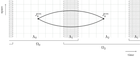
Figure 1: Domain decomposition of the lattice adopted in this paper. Periodic (anti-periodic) boundary conditions in the time direction are enforced for gluons (fermions).

The next step consists in rewriting the determinant of the Hermitean massive Wilson-Dirac operator $Q=\gamma_{5}D$ as

$$\det\,Q=\frac{\det\,\left(1-w\right)}{\det\,Q_{\Lambda_{1}}\det\,Q^{-1}_{\Omega_{0}}\det\,Q^{-1}_{\Omega_{2}}}\;,$$ (5)

where $Q_{\Lambda_{1}}$, $Q_{\Omega_{0}}$, and $Q_{\Omega_{2}}$ indicate the very same operator restricted to the domains specified by the subscript. They are obtained from $Q$ by imposing Dirichlet boundary conditions on the external boundaries of each domain. The matrix $w$ is

$$w=P_{\partial\Lambda_{0}}Q^{-1}_{\Omega_{0}}\,Q_{\Lambda_{1,2}}\,Q^{-1}_{\Omega_{2}}Q_{\Lambda_{1,0}}\,,$$ (6)

where $Q_{\Lambda_{1,0}}$ and $Q_{\Lambda_{1,2}}$ are the hopping terms of the operator $Q$ across the boundaries in between the inner domains $\Lambda_{0}$ and $\Lambda_{2}$ and the common region $\Lambda_{1}$ respectively, while $P_{\partial\Lambda_{0}}$ is the projector on the inner boundary of $\Lambda_{0}$ [17]. The denominator in Eq. (5) has already a factorized dependence on the gauge field since $\det Q_{\Lambda_{1}}$, $\det\,Q^{-1}_{\Omega_{0}}$ and $\det\,Q^{-1}_{\Omega_{2}}$ depend only on the gauge field in $\Lambda_{1}$, $\Omega_{0}$ and $\Omega_{2}$ respectively.

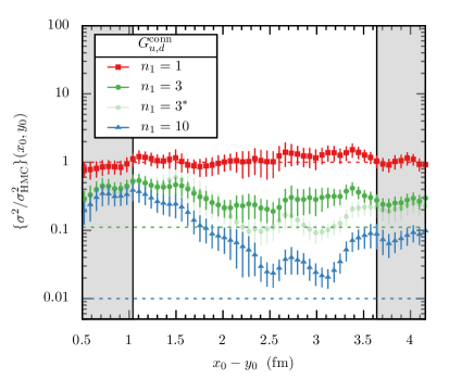
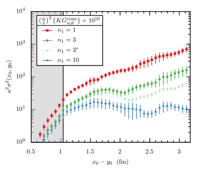
Figure 2: Left: variance of the light-connected contraction as a function of the difference between the time-coordinates of the currents for $n_{1}=1,3,10$ ($n_{1}=3^{*}$ is obtained by skipping $48$ MDUs between two consecutive level-$1$ configurations). Data are normalized to the analogous ones computed on CLS configurations generated by one-level HMC. Dashed lines represent the maximum reduction which can be obtained by two-level integration, namely $1/n^{2}_{1}$, in the absence of correlations between level-$1$ configurations. Grey bands indicate the thick time-slices where the gauge field is kept fixed during level-$1$ updates. Right: variance of the light-connected contribution to the integrand in Eq. (1).

In the last step, the numerator in Eq. (5) is rewritten as

$$\det\,\left(1-w\right)=\frac{\det\,[1-R_{N+1}(1-w)]}{C\prod_{k=1}^{N/2}{\det}\big{[}(u_{k}-w)^{\dagger}(u_{k}-w)\big{]}}\,,$$ (7)

where $u_{k}$ and $u^{*}_{k}$ are the $N$ roots of a polynomial approximant for $(1-w)^{-1}$, the numerator is the remainder, and $C$ is an irrelevant constant. The denominator in Eq. (7) can be represented by an integral over a set of $N/2$ multi-boson fields [22, 23] having an action with a factorized dependence on the gauge field in $\Lambda_{0}$ and $\Lambda_{2}$  [16, 17, 18] inherited from $w$. When the polynomial approximation is properly chosen, see below, the remainder in the numerator of Eq. (7) has mild fluctuations in the gauge field, and is included in the observable in the form of a reweighting factor in order to obtain unbiased estimates.

A simple implementation of these ideas is to divide the lattice as shown in Fig. 1, where $\Lambda_{0}$ and $\Lambda_{2}$ have the shape of thick time-slices while $\Lambda_{1}$ includes the remaining parts of the lattice. The short-distance suppression of the quark propagator implies that a thickness of $0.5$ fm or so for the thick-time slices forming $\Lambda_{1}$ is good enough, see e.g. Fig. 4 in Ref. [24], and is not expected to vary significantly with the quark mass. This is the domain decomposition that we use for the numerical computations presented in this letter.

The Monte Carlo simulation is then performed using a two-level scheme. We first generate $n_{0}$ level-$0$ gauge field configurations by updating the field over the entire lattice; then, starting from each level-$0$ configuration, we keep fixed the gauge field in the overlapping region $\Lambda_{1}$, and generate $n_{1}$ level-$1$ configurations by updating the field in $\Lambda_{0}$ and in $\Lambda_{2}$ independently thanks to the factorization of the action. The resulting gauge fields are then combined to obtain effectively $n_{0}\cdot n_{1}^{2}$ configurations at the cost of generating $n_{0}\cdot n_{1}$ gauge fields over the entire lattice. In particular, for each level-$0$ configuration, we compute the statistical estimators by averaging the values of the correlators over the $n_{1}^{2}$ level-$1$ gauge fields. Previous experience on two-level integration [25, 26, 16, 17] suggests that, with two independently updated regions, the variance decreases proportionally to $1/n_{1}^{2}$ until the standard deviation of the estimator is comparable with the signal, i.e. until the level-$1$ integration has solved the signal-to-noise problem. From Eq. (4) we thus infer that the variance reduction due to level-$1$ integration is expected to grow exponentially with the time-distance of the currents in Eq. (2). The overhead for simulating the extra multi-boson fields increases the cost by an overall constant factor which is quickly amortized by the improved scaling.

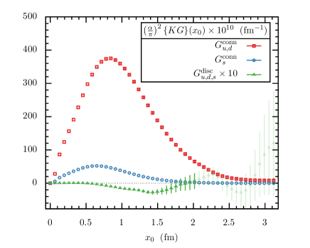
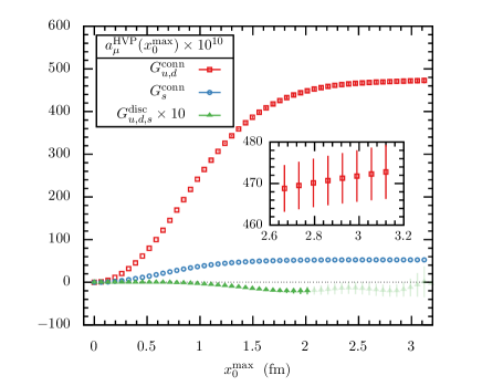
Figure 3: Left: best results for the contribution to the integrand in Eq. (1) from the light-connected (red squares), strange-connected (blue circles) and disconnected (green triangles) contractions as a function of the time coordinate. Right: best results for the contributions to $a_{\mu}^{\rm HVP}$ from light-connected (red squares), strange-connected (blue circles), and disconnected (green triangles) contractions as a function of the upper extrema of integration $x_{0}^{\rm max}$.

4 Lattice computation

In order to assess the potential of two-level Monte Carlo integration, we simulate QCD with two dynamical flavours supplemented by a valence strange quark. Gluons are discretized by the Wilson action while quarks by the $O(a)$-improved Wilson–Dirac operator, see Refs. [27, 18] for unexplained definitions. Periodic and anti-periodic boundary conditions are imposed on the gluon and fermion fields in the time direction respectively, while periodic conditions are chosen for all fields in the spatial directions. We simulate a lattice of size $96\times 48^{3}$ with an inverse bare coupling constant $\beta=6/g_{0}^{2}=5.3$, corresponding to a spacing of $\;a=0.065$ fm [28, 27]. The size of the lattice, rather large for a proof of concept, is chosen so to be able to accommodate a light pion and still be in the large volume regime, namely $M_{\pi}=270$ MeV and $M_{\pi}L\geq 4$. The domains $\Lambda_{0}$ and $\Lambda_{2}$ are the union of $40$ consecutive time-slices, while each thick time-slice forming the overlapping region $\Lambda_{1}$ is made of $8$ time-slices corresponding to a thickness of approximately $0.5$ fm. The determinants in the denominator of Eq. (5) are taken into account by standard pseudofermion representations, while the number of multi-bosons is fixed to $N=12$. The very same action and set of auxiliary fields are used either at level-$0$ or level-$1$. The reweighting factor is estimated stochastically with 2 random sources, which are enough for its contribution to the statistical error to be negligible. Further details on the algorithm and its implementation can be found in Ref. [18].

We generate $n_{0}=25$ level-0 configurations separated by $48$ molecular dynamics units (MDU), so that in practice they can be considered statistically uncorrelated [28, 27]. For each level-$0$ background gauge field, we generate $n_{1}=10$ configurations in $\Lambda_{0}$ and $\Lambda_{2}$ spaced by $16$ MDUs. The connected contraction is calculated by inverting the Wilson-Dirac operator on local sources, while the disconnected one is computed via split-even random-noise estimators [29]. For each level-$0$ configuration, the statistical estimators are computed by averaging the correlators over the $n_{1}^{2}$ combinations of level-$1$ fields. The error analysis then proceeds as usual. For the sake of the presentation, we show results in physical units and properly renormalized: the central value of the lattice spacing is taken from Ref. [27], and the one of the vector-current renormalization constant from Ref. [30]. We do not take into account their contributions to the errors since on one side we are interested in investigating the statistical precision of the vector correlator computed via two-level integration only, and on the other side the numerical accuracy of those quantities can be improved independently.

To single out the reduction of the variance due only to two-level averaging, we carry out a dedicated calculation of correlation functions. We compute the light-connected contraction by averaging over $216$ local sources put on the time-slice ($y_{0}/a=32$) of $\Lambda_{0}$ at a distance of $8$ lattice spacings from its right boundary and, as usual, by summing over the sink space-position. This large number of sources guarantees that the dependence of the variance on the gauge field in the domains $\Lambda_{0}$ and $\Lambda_{2}$ is on equal footing, since no further significant variance reduction is observed by increasing their number. We determine the disconnected contraction by averaging each single-propagator trace over a large number of Gaussian random sources, namely $768$, so to have a negligible random-noise contribution to the variance [29].

The variance of the light-connected contribution as a function of the distance from the source is shown on the left plot of Fig. 2. For better readability only the time-slices belonging to $\Omega_{2}$ are shown, i.e. those relevant for studying the effect of two-level integration given the source position. Data are normalized to the variance obtained with the same number of sources on CLS configurations which were generated with a conventional one-level HMC [31, 32, 28]. The exponential reduction of the variance with the distance from the source is manifest in the data, with the maximum gain reached from $2.5$ fm onward for $n_{1}=10$. The loss of about a factor between $2$ and $3$ with respect to the best possible scaling, namely $n_{1}^{2}$, either for $n_{1}=3$ or $10$ (dashed lines) is compatible with the presence of a residual correlation among level-$1$ configurations. Indeed the variance reduction for $n_{1}=3$, obtained by skipping $48$ MDUs between consecutive level-$1$ configurations (labeled by $n_{1}=3^{*}$), is compatible with the $n_{1}^{2}$ scaling at large distances within errors. In our particular setup, even for $n_{1}=10$ the statistical error at large distances scales de-facto with the inverse of the cost of the simulation rather than with its squared root. This is easily seen by comparing the variance reduction shown in the left plot of Fig. 2 with the cost of the simulation for $n_{1}=10$. The latter is in fact $4$ times the one for $n_{1}=1$ due to the different separation in MDU units between two consecutive configurations at level-$0$ and level-$1$.
The power of the two-level integration can be better appreciated from the right plot of Fig. 2, where we show the variance of the light-connected contribution to the integrand in Eq. (1) as a function of the time-distance of the currents. The sharp rising of the variance computed by one-level Monte Carlo ($n_{1}=1$, red squares) is automatically flattened out by the two-level multi-boson domain-decomposed HMC ($n_{1}=10$, blue triangles) without the need for modeling the long-distance behaviour of $G^{\rm conn}_{u,d}(x_{0})$.

To further appreciate the effect of the two-level integration, we compute the integral in Eq. (1) as a function of the upper extrema of integration $x_{0}^{\rm max}$ which we allow to vary. For $n_{1}=1$, the integral reads $446(26)$ and $424(38)$ for $x_{0}^{\rm max}=2.5$ and $3.0$ fm respectively, while for $n_{1}=10$ the analogous values are $467.0(8.4)$ and $473.4(8.6)$. While with the one-level integration the errors on the contributions to the integral from $0$ to $2.5$ fm and from $2.5$ to the maximum value of $3.0$ fm are comparable, with the two-level HMC the contribution to the variance from the long distance part becomes negligible. This pattern of variance reduction is expected to set in at shorter distances for lighter quark masses, where the gain due to the two-level integration is expected to be significantly larger due to the sharp increase of the exponential in Eq. (4). Considerations analogous to those made for the connected contribution apply also to the much smaller disconnected one, although even larger values of $n_{1}$ are required to render the variance approximately constant.

5 Results and discussion

Our best result for the light-connected contribution to the integrand in Eq. (1) is shown on the left plot of Fig. 3 (red squares). It is obtained by a weighted average of the above discussed correlation function computed on $32$ point sources per time-slice on $7$ time-slices at $y_{0}/a=\{8,16,24,56,64,72,80\}$ and on $216$ sources at $y_{0}/a=32$. We obtain a good statistical signal up to the maximum distance of $3$ fm or so. The strange-connected contraction $G^{\rm conn}_{s}(x_{0})$ is much less noisy, and is determined by averaging on $16$ point sources at $y_{0}/a=32$. Its value, shown on the left plot of Fig. 3 (blue circles), is at most one order of magnitude smaller than the light contribution, and has a negligible statistical error with respect to the light one. The best result for the disconnected contribution has been computed as discussed in the previous section, and it is shown in the left plot of Fig. 3 as well (green triangles). It reaches a negative peak at about $1.5$ fm, and a good statistical signal is obtained up to $2.0$ fm or so. Its absolute value is more than two orders of magnitude smaller than the light-connected contribution over the entire range explored (notice the multiplication by $10$ for a better readability of the plot).
In the right plot of Fig. 3 we show the best values of the light-connected (red squares), strange-connected (blue circles), and disconnected (green triangles) contributions to $a_{\mu}^{\rm HVP}\cdot 10^{10}$ as a function of the upper extrema of integration $x_{0}^{\rm max}$ in Eq. (1). The light-connected part starts to flatten out at $x_{0}^{\rm max}\sim 2.5$ fm and, at the conservative distance of $x_{0}^{\rm max}=3.0$ fm, its value is $471.8(6.2)$. The value of the strange-connected contribution is $52.55(21)$ at $x_{0}^{\rm max}=3.0$ fm, and its error is negligible with respect to the light-connected one. The disconnected contribution starts to flatten out at about $x_{0}^{\rm max}\sim 2.0$ fm, where its value is $-1.98(84)$. For $x_{0}^{\rm max}=3.0$ fm, its statistical uncertainty is $2.1$ which is still 3 times smaller with respect to the light-connected one. Clearly the disconnected contribution must be taken into account to attain a per-mille precision on the HVP, but the combined usage of split-even estimators and two-level integration solves the problem of its computation. By combining the connected contributions at $x_{0}^{\rm max}=3.0$ fm with the disconnected part at $x_{0}^{\rm max}=2.0$ fm, the best total value that we obtain is $a_{\mu}^{\rm HVP}=522.4(6.2)\cdot 10^{-10}$.
In this proof of concept study we have achieved a 1% statistical precision with just $n_{0}\cdot n_{1}=250$ configurations on a realistic lattice. This shows that for this light-quark mass a per-mille statistical precision on $a_{\mu}^{\rm HVP}$ is reachable with multi-level integration by increasing $n_{0}$ and $n_{1}$ by a factor of about $4$–$6$ and $2$–$4$ respectively. When the up and the down quarks become lighter, the gain due to the multi-level integration is expected to increase exponentially in the quark mass, hence improving even more dramatically the scaling of the simulation cost with respect to a standard one-level Monte Carlo. The change of computational paradigm presented here thus removes the main barrier for making affordable, on the computer installations available today, the goal of a per-mille precision on $a_{\mu}^{\rm HVP}$.
Here we focused on the main bottleneck in the computation of the HVP. It goes without saying that the very same variance-reduction pattern is expected to work out also for the calibration of the lattice spacing, the calculation of the electromagnetic corrections and the HLbL.
It is also interesting to notice that multi-level integration can be well integrated with master-field simulation techniques [33] if very large volumes turn out to be necessary to pin down finite-size effects at the per-mille level. As a final remark, we stress that the very same approach is applicable to many other computations which suffer from signal-to-noise ratio problems, where a similar breakthrough is expected [34].

6 Acknowledgments

The generation of the configurations and the measurement of the correlators have been performed on the PC clusters Marconi at CINECA (CINECA- INFN, CINECA-Bicocca agreements, ISCRA B project HP10BF2OQT) and at the Juelich Supercomputing Centre, Germany (PRACE project n. 2019215140) while the R&D has been carried out on Wilson and Knuth at Milano-Bicocca. We thank these institutions and PRACE for the computer resources and the technical support. We also acknowledge PRACE for awarding us access to MareNostrum at Barcelona Supercomputing Center (BSC), Spain (n. 2018194651) where comparative performance tests of the code have been performed. We acknowledge partial support by the INFN project “High performance data network”.

References

- [1] G. W. Bennett, et al., Final Report of the Muon E821 Anomalous Magnetic Moment Measurement at BNL, Phys. Rev. D73 (2006) 072003. arXiv:hep-ex/0602035, doi:10.1103/PhysRevD.73.072003.
- [2] J. Grange, et al., Muon (g-2) Technical Design ReportarXiv:1501.06858.
- [3] Abe, M. et al. (J-PARC g-2/EDM Collab., http://g-2.kek.jp), A New Approach for Measuring the Muon Anomalous Magnetic Moment and Electric Dipole Moment, PTEP 2019 (5) (2019) 053C02. arXiv:1901.03047, doi:10.1093/ptep/ptz030.
- [4] T. Aoyama, et al., The anomalous magnetic moment of the muon in the Standard Model, Phys. Rept. 887 (2020) 1–166. arXiv:2006.04822, doi:10.1016/j.physrep.2020.07.006.
- [5] G. Abbiendi, et al., Measuring the leading hadronic contribution to the muon g-2 via scattering, Eur. Phys. J. C 77 (3) (2017) 139. arXiv:1609.08987, doi:10.1140/epjc/s10052-017-4633-z.
- [6] T. Blum, P. A. Boyle, V. Gülpers, T. Izubuchi, L. Jin, C. Jung, A. Jüttner, C. Lehner, A. Portelli, J. T. Tsang, Calculation of the hadronic vacuum polarization contribution to the muon anomalous magnetic moment, Phys. Rev. Lett. 121 (2) (2018) 022003. arXiv:1801.07224, doi:10.1103/PhysRevLett.121.022003.
- [7] D. Giusti, V. Lubicz, G. Martinelli, F. Sanfilippo, S. Simula, Electromagnetic and strong isospin-breaking corrections to the muon from Lattice QCD+QED, Phys. Rev. D 99 (11) (2019) 114502. arXiv:1901.10462, doi:10.1103/PhysRevD.99.114502.
- [8] C. Davies, et al., Hadronic-vacuum-polarization contribution to the muon’s anomalous magnetic moment from four-flavor lattice QCD, Phys. Rev. D 101 (3) (2020) 034512. arXiv:1902.04223, doi:10.1103/PhysRevD.101.034512.
- [9] E. Shintani, Y. Kuramashi, Hadronic vacuum polarization contribution to the muon with 2+1 flavor lattice QCD on a larger than (10 fm lattice at the physical point, Phys. Rev. D100 (3) (2019) 034517. arXiv:1902.00885, doi:10.1103/PhysRevD.100.034517.
- [10] A. Gérardin, M. Cè, G. von Hippel, B. Hörz, H. B. Meyer, D. Mohler, K. Ottnad, J. Wilhelm, H. Wittig, The leading hadronic contribution to from lattice QCD with flavours of O() improved Wilson quarks, Phys. Rev. D100 (1) (2019) 014510. arXiv:1904.03120, doi:10.1103/PhysRevD.100.014510.
- [11] C. Aubin, T. Blum, C. Tu, M. Golterman, C. Jung, S. Peris, Light quark vacuum polarization at the physical point and contribution to the muon , Phys. Rev. D101 (1) (2020) 014503. arXiv:1905.09307, doi:10.1103/PhysRevD.101.014503.
- [12] S. Borsanyi, et al., Leading-order hadronic vacuum polarization contribution to the muon magnetic moment from lattice QCDarXiv:2002.12347.
- [13] M. Passera, W. J. Marciano, A. Sirlin, The Muon g-2 and the bounds on the Higgs boson mass, Phys. Rev. D 78 (2008) 013009. arXiv:0804.1142, doi:10.1103/PhysRevD.78.013009.
- [14] A. Keshavarzi, W. J. Marciano, M. Passera, A. Sirlin, Muon and connection, Phys. Rev. D 102 (3) (2020) 033002. arXiv:2006.12666, doi:10.1103/PhysRevD.102.033002.
- [15] A. Crivellin, M. Hoferichter, C. A. Manzari, M. Montull, Hadronic Vacuum Polarization: versus Global Electroweak Fits, Phys. Rev. Lett. 125 (9) (2020) 091801. arXiv:2003.04886, doi:10.1103/PhysRevLett.125.091801.
- [16] M. Cè, L. Giusti, S. Schaefer, Domain decomposition, multi-level integration and exponential noise reduction in lattice QCD, Phys. Rev. D93 (9) (2016) 094507. arXiv:1601.04587, doi:10.1103/PhysRevD.93.094507.
- [17] M. Cè, L. Giusti, S. Schaefer, A local factorization of the fermion determinant in lattice QCD, Phys. Rev. D95 (3) (2017) 034503. arXiv:1609.02419, doi:10.1103/PhysRevD.95.034503.
- [18] M. Dalla Brida, L. Giusti, T. Harris, M. Pepe, in preparation.
- [19] D. Bernecker, H. B. Meyer, Vector Correlators in Lattice QCD: Methods and applications, Eur. Phys. J. A47 (2011) 148. arXiv:1107.4388, doi:10.1140/epja/i2011-11148-6.
- [20] M. Della Morte, A. Francis, V. Gülpers, G. Herdoíza, G. von Hippel, H. Horch, B. Jäger, H. B. Meyer, A. Nyffeler, H. Wittig, The hadronic vacuum polarization contribution to the muon from lattice QCD, JHEP 10 (2017) 020. arXiv:1705.01775, doi:10.1007/JHEP10(2017)020.
- [21] V. Gülpers, Recent Developments of Muon g-2 from Lattice QCD, PoS LATTICE2019 (2020) 224. arXiv:2001.11898, doi:10.22323/1.363.0224.
- [22] M. Lüscher, A New approach to the problem of dynamical quarks in numerical simulations of lattice QCD, Nucl. Phys. B418 (1994) 637–648. arXiv:hep-lat/9311007, doi:10.1016/0550-3213(94)90533-9.
- [23] A. Borici, P. de Forcrand, Systematic errors of Lüscher’s fermion method and its extensions, Nucl. Phys. B454 (1995) 645–662. arXiv:hep-lat/9505021, doi:10.1016/0550-3213(95)00429-V.
- [24] M. Lüscher, Lattice QCD and the Schwarz alternating procedure, JHEP 05 (2003) 052. arXiv:hep-lat/0304007, doi:10.1088/1126-6708/2003/05/052.
- [25] M. Lüscher, P. Weisz, Locality and exponential error reduction in numerical lattice gauge theory, JHEP 09 (2001) 010. arXiv:hep-lat/0108014, doi:10.1088/1126-6708/2001/09/010.
- [26] M. Della Morte, L. Giusti, A novel approach for computing glueball masses and matrix elements in Yang-Mills theories on the lattice, JHEP 05 (2011) 056. arXiv:1012.2562, doi:10.1007/JHEP05(2011)056.
- [27] G. P. Engel, L. Giusti, S. Lottini, R. Sommer, Spectral density of the Dirac operator in two-flavor QCD, Phys. Rev. D91 (5) (2015) 054505. arXiv:1411.6386, doi:10.1103/PhysRevD.91.054505.
- [28] P. Fritzsch, F. Knechtli, B. Leder, M. Marinkovic, S. Schaefer, R. Sommer, F. Virotta, The strange quark mass and Lambda parameter of two flavor QCD, Nucl. Phys. B865 (2012) 397–429. arXiv:1205.5380, doi:10.1016/j.nuclphysb.2012.07.026.
- [29] L. Giusti, T. Harris, A. Nada, S. Schaefer, Frequency-splitting estimators of single-propagator traces, Eur. Phys. J. C79 (7) (2019) 586. arXiv:1903.10447, doi:10.1140/epjc/s10052-019-7049-0.
- [30] M. Dalla Brida, T. Korzec, S. Sint, P. Vilaseca, High precision renormalization of the flavour non-singlet Noether currents in lattice QCD with Wilson quarks, Eur. Phys. J. C79 (1) (2019) 23. arXiv:1808.09236, doi:10.1140/epjc/s10052-018-6514-5.
- [31] L. Del Debbio, L. Giusti, M. Lüscher, R. Petronzio, N. Tantalo, QCD with light Wilson quarks on fine lattices (I): First experiences and physics results, JHEP 02 (2007) 056. arXiv:hep-lat/0610059, doi:10.1088/1126-6708/2007/02/056.
- [32] L. Del Debbio, L. Giusti, M. Lüscher, R. Petronzio, N. Tantalo, QCD with light Wilson quarks on fine lattices. II. DD-HMC simulations and data analysis, JHEP 02 (2007) 082. arXiv:hep-lat/0701009, doi:10.1088/1126-6708/2007/02/082.
- [33] A. Francis, P. Fritzsch, M. Lüscher, A. Rago, Master-field simulations of O(a)-improved lattice QCD: Algorithms, stability and exactness, Comput. Phys. Commun. 255 (2020) 107355. arXiv:1911.04533, doi:10.1016/j.cpc.2020.107355.
- [34] L. Giusti, M. Cè, S. Schaefer, Multi-boson block factorization of fermions, EPJ Web Conf. 175 (2018) 01003. arXiv:1710.09212, doi:10.1051/epjconf/201817501003.