Kinematic modelling of clusters with Gaia:
the Death Throes of the Hyades

Abstract

The precision of the Gaia data offers a unique opportunity to study the internal velocity field of star clusters. We develop and validate a forward-modelling method for the internal motions of stars in a cluster. The model allows an anisotropic velocity dispersion matrix and linear velocity gradient describing rotation and shear, combines radial velocities available for a subset of stars, and accounts for contamination from background sources via a mixture model. We apply the method to Gaia DR2 data of the Hyades cluster and its tidal tails, dividing and comparing the kinematics of stars within and beyond $10$ pc, which is roughly the tidal radius of the cluster. While the velocity dispersion for the cluster is nearly isotropic, the velocity ellipsoid for the tails is clearly elongated with the major axis pointing towards the Galactic centre. We find positive and negative expansion at $\approx 2\sigma$ significance in Galactic azimuthal and vertical direction for the cluster but no rotation. The tidal tails are stretching in a direction tilted from the Galactic centre while equally contracting as the cluster in Galactic vertical direction. The tails have a shear ($A$) of $16.90\pm 0.92$ $\mathrm{m}\,\mathrm{s}^{-1}\,\mathrm{pc}^{-1}$and a vorticity ($B$) of $-6.48\pm 1.15$ $\mathrm{m}\,\mathrm{s}^{-1}\,\mathrm{pc}^{-1}$, values distinct from the local Oort constants. By solving the Jeans equations for flattened models of the Hyades, we show that the observed velocity dispersions are a factor of $\approx 2$ greater than required for virial equilibrium due to tidal heating and disruption. From simple models of the mass loss, we estimate that the Hyades is close to final dissolution with only a further $\lesssim 30$ Myr left.

Section 1 Introduction

Stars are born in supersonically-turbulent, self-gravitating Giant Molecular Clouds, which are hierarchically structured. Dense regions within a cloud, often referred to as “clumps”, are thought to be birth sites of star clusters (Krumholz et al., 2019, and references therein). Although both the molecular clouds and the clumps within them are gravitationally bound (Heyer & Dame, 2015; Urquhart et al., 2018), only $\lesssim 10$% of the initial stellar groups observed in the distribution of young stellar objects eventually become bound star clusters after gas removal (Lada & Lada, 2003). The pathway by which stellar groups emerging from the hierarchical structure of a cloud end up as bound clusters is not well understood.

Once formed, the evolution of bound star clusters is governed by both internal processes, such as stellar and binary evolution, mass segregation and two body relaxation effects, as well as external influences, such as galactic tides, bulge and disc shocking, and gravitational interactions with passing molecular clouds. The complex interplay between internal and external effects leads to the death throes of many star clusters. For example, tidal disruption may be enhanced by stellar evolution, leading to mass loss through winds and supernova explosions. This reduces the density in a cluster and makes it more fragile to the buffetings of external tidal forces.

Studies of internal kinematics of clusters and associations can provide critical and direct insights into their formation and evolution, which are orthogonal to existing constraints such as morphology and stellar demographics. As internal motions are differences of velocities with respect to the mean motion and star clusters typically have velocity dispersions (a proxy for the magnitude of internal motions) of less than a few $\rm km~{}s^{-1}$, their study requires high-precision astrometric measurements in order to pin down the positions, velocities and membership of clusters. Until recently, such studies were limited to a few nearby star-forming regions and specifically targeted surveys of clusters.

The Gaia mission (Gaia Collaboration et al., 2016) has changed the situation dramatically, as it delivers astrometry for over a billion sources brighter than $G=20$ and radial velocities for a subset of brighter stars ($G<12$). Indeed, the Gaia second data release (Gaia Collaboration et al., 2018a, GDR2) has already fueled a number of studies on the internal kinematics of clusters and associations.

Indeed, many recent studies have already examined the internal kinematics of young ($\lesssim 30$ Myr) associations in large star-forming complexes (Zari et al., 2019; Kim et al., 2019; Kuhn et al., 2019; Kounkel et al., 2018; Kos et al., 2019; Wright & Mamajek, 2018; Cantat-Gaudin et al., 2019; Wright et al., 2019) with particular interest in the role of gas expulsion from stellar feedback. The results are varied from subgroups in the Scorpius-Centaurus OB association showing no expansion (Wright & Mamajek, 2018) to groups in the Vela Puppis region and the Lagoon Nebula showing anisotropic expansion (Cantat-Gaudin et al., 2019; Wright et al., 2019). An emerging picture is that star formation in these regions produces highly substructured and complex distribution of young stars, and involves multiple episodes of star forming events.

Here, we present a forward-modelling approach to the kinematic modelling of clusters suited for taking full advantage of the combination of the Gaia astrometry with radial velocities from various spectroscopic surveys. Our method builds upon and extends the work of Lindegren et al. (2000), which was developed to infer the astrometric radial velocities from the Hipparcos data (see also Reino et al., 2018; Bravi et al., 2018; Zari et al., 2019, for its applications to the Gaia data). We describe and justify each components of our model, and validate our implementation with mock data generated according to the model in Section 2.

We apply the method to the specific example of the Hyades cluster in Section 3. This is one of the nearest ($d\approx 46$ pc), large ($N\gtrsim 500$ for $G\lesssim 20$), old ($\approx 680$ Myr; Gossage et al., 2018) open clusters. Historically, the Hyades cluster played an important role as a calibrator of the absolute magnitude-spectral type and the mass-luminosity relation. Modern interest in the Hyades is focused on the cluster’s birth, life and death in the Galactic environment. Its proximity to the Sun and thus the availability of high quality astrometric data has stimulated a number of kinematical studies, from Hipparcos  (Perryman et al., 1998; de Bruijne et al., 2001) to the first Gaia data release (Reino et al., 2018). Very recently, GDR2 has revealed the existence of tidal tails of the cluster out to $\lesssim 150$ pc from the cluster centre (Meingast & Alves, 2019; Röser et al., 2019). Section 4 builds steady-state and evolving models of the Hyades cluster in the light of our kinematic investigations. We discuss the results in the context of complete tidal dissolution of the cluster.

Section 2 Method

Parameter	Description	Prior	Unit
$N$	total number of stars in the sample
$N_{\mathrm{RV}}$	total number of stars with radial velocities
$i$	star index, $i=1,\dots,N$
$\boldsymbol{v}_{0}$	mean velocity vector $(v_{x},\,v_{y},\,v_{z})$ in ICRS	$\mathcal{N}(0,\,50)$	$\rm km~{}s^{-1}$
$\mathbf{\Sigma}$	(3, 3) velocity dispersion matrix of the cluster, $\Sigma=\mathrm{diag}(\boldsymbol{\sigma}_{v})\,\mathbf{\Omega}\,\mathrm{diag}(\boldsymbol{\sigma}_{v})$		$\mathrm{km}^{2}\,\mathrm{s}^{-2}$
$\boldsymbol{\sigma}_{v}$	scale vector of $\Sigma$	$\text{Half-Cauchy}(0,\,2.5)$	$\rm km~{}s^{-1}$
$\mathbf{\Omega}$	correlation matrix of $\Sigma$	$\mathrm{LKJ}(2)$
$\mathbf{T}$	velocity gradient matrix, $T_{ij}=dv_{i}/dx_{j}$	$\mathcal{N}(0,\,50)$	$\mathrm{m}\,\mathrm{s}^{-1}\,\mathrm{pc}^{-1}$
$f_{\mathrm{mem}}$	fraction of the sample that are cluster members	$\mathcal{U}(0,\,1)$
$\sigma_{\mathrm{bg}}$	velocity dispersion of the background	$\mathcal{N}(30,\,20)$, $\sigma_{\mathrm{bg}}>0$	$\rm km~{}s^{-1}$
$\boldsymbol{v}_{0,\mathrm{bg}}$	mean velocity of the background	$\mathcal{N}(0,\,50)$,	$\rm km~{}s^{-1}$
$d_{i}$	distance of star $i$		pc
$\boldsymbol{v}_{i}$	velocity vector of star $i$		$\rm km~{}s^{-1}$
$\alpha_{i}$, $\delta_{i}$	right ascension and declination of star $i$	fixed	deg, deg
$\boldsymbol{a}_{i}$	astrometry vector $(\pi,\,\mu_{\alpha},\,\mu_{\delta})$ for star $i$	observed	$(\mathrm{mas},\,{\mathrm{mas}\,\mathrm{yr}^{-1}},\,{\mathrm{mas}\,\mathrm{yr}^{-1}})$
$\mathbf{C}_{\boldsymbol{a},i}$	noise covariance matrix of $\boldsymbol{a}$ for star $i$	fixed
$v_{r,i}$	radial velocity	observed	$\rm km~{}s^{-1}$
$\sigma_{\mathrm{RV},i}$	radial velocity error	fixed	$\rm km~{}s^{-1}$

Table 1: Summary of parameters and prior specifications for the model.

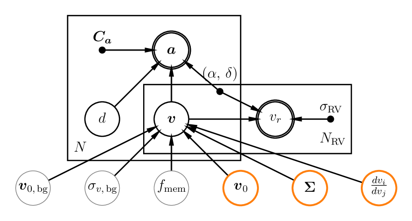
Figure 1: Probabilistic graphical model for cluster internal kinematics. The key parameters of interest – mean velocity, velocity dispersion matrix and velocity gradient matrix – are highlighted in thick orange circles, whereas the nuisance parameters – mean velocity and (isotropic) velocity dispersion of the background, and the fraction of stars that are members – are in thin gray circles. The observables (in double-lined circles) are the vectors $\boldsymbol{a}=(\pi,\,\mu_{\alpha},\,\mu_{\delta})$ and radial velocities $v_{r}$ when available. Note that the uncertainty covariances between parallax and proper motions, $\mathbf{C}_{\boldsymbol{a},i}$, and uncertainties of radial velocities, $\sigma_{\mathrm{RV}}$ are taken into account. See Section 2.1 for details.

2.1 Model

Our model of the velocity field of cluster members includes linear velocity gradients describing rotation and shear, and the full dispersion matrix as well as contamination by kinematic outliers. Figure 1 provides a visual summary as a probabilistic graphical model. All parameters and their priors (if any) are recorded in Table 1.

Traditionally, the velocities of stars in a cluster are assumed to be the same with a small, usually isotropic, dispersion. This assumption has been utilized in mainly two different ways. If we have proper motions and radial velocities (RVs) of the members, we can deduce the mean distance (parallax) of the cluster (“moving cluster method”). On the other hand, if we have parallaxes and proper motions, we can infer the mean and individual radial velocities. The radial velocities derived in such a way are referred to as “astrometric” radial velocities in order to differentiate them from the more common spectroscopic radial velocities from Doppler shifts (Dravins et al., 1999). However, as discussed in the introduction, it is more interesting in the Gaia-era to explore internal motions beyond this simple model for clues as to the birth conditions or evolution of the cluster. We can do this by combining precise astrometry with radial velocity measurements, which are often only available for a portion of the astrometric sample.

The velocity of a member star $i$ in a cluster, $\boldsymbol{v}_{i}$, is assumed to be the sum of the mean velocity $\boldsymbol{v}_{0}$ of the cluster, systematic peculiar velocity, and some scatter (dispersion), which is expected to be small ($\lesssim$ few $\rm km~{}s^{-1}$). Systematic internal motions such as rotation or shear are captured by the linear velocity gradients $\mathbf{T}=T_{lk}=dv_{l}/dx_{k}$ to first approximation (Lindegren et al., 2000). The anti-symmetric part of $\mathbf{T}$ describes the rigid body rotation, and the symmetric part describes the extensional (contraction or expansion) and shear strain rates, which can be diagonalized to examine the principal axes of shear:

$$\frac{1}{2}(\mathbf{T}-\mathbf{T}^{T})=\begin{bmatrix}0&-\omega_{z}&\omega_{y}\\ \omega_{z}&0&-\omega_{x}\\ -\omega_{y}&\omega_{x}&0\end{bmatrix};\,\,\begin{split}\omega_{x}&=\frac{1}{2}(T_{zy}-T_{yz})\\ \omega_{y}&=\frac{1}{2}(T_{xz}-T_{zx})\\ \omega_{z}&=\frac{1}{2}(T_{yx}-T_{xy})\end{split}$$ (1)

$$\frac{1}{2}(\mathbf{T}+\mathbf{T}^{T})=\begin{bmatrix}w_{4}&w_{3}&w_{2}\\ w_{3}&w_{5}&w_{1}\\ w_{2}&w_{1}&3\kappa-w_{4}-w_{5}\end{bmatrix};\,\,\begin{split}w_{1}&=\frac{1}{2}(T_{zy}+T_{yz})\\ w_{2}&=\frac{1}{2}(T_{xz}+T_{zx})\\ w_{3}&=\frac{1}{2}(T_{yx}+T_{xy})\\ w_{4}&=T_{xx}\\ w_{5}&=T_{yy}\\ \kappa&=\frac{1}{3}(T_{xx}+T_{yy}+T_{zz})\end{split}$$ (2)

Here, $\omega_{\{x,\,y,\,z\}}$ is the rotation around each axis and we have followed the notation of Lindegren et al. (2000) to use $w_{1},\ldots,w_{5}$ and $\kappa$ for the components of the symmetric shear matrix.

It is well-known that there is a degeneracy between mean velocity and the isotropic expansion/contraction component $\kappa$ when considering astrometry alone (Blaauw, 1964; Dravins et al., 1999). Generally, only 8 of 9 components of velocity gradient matrix $\mathbf{T}$ can be determined from astrometry alone and there still exists one-dimensional degeneracy due to lack of information on how radial velocities change. By incorporating all radial velocities available for a subset of bright stars in GDR2, we can break the degeneracy and infer all nine components of $\mathbf{T}$ that is most consistent with the data.

We make the velocity dispersion a general symmetric matrix, $\mathbf{\Sigma}$, in order to test the assumption of isotropic dispersion in light of Gaia data. Indeed, recent studies of young clusters including the Orion Nebula Cluster have already reported anisotropic on-sky velocity dispersions with GDR2 (Kuhn et al., 2019; Kim et al., 2019; Wright et al., 2019). We decompose $\mathbf{\Sigma}$ into a scale vector $\boldsymbol{\sigma}_{v}$ and correlation matrix $\mathbf{\Omega}$, such that $\Sigma=\mathrm{diag}(\boldsymbol{\sigma}_{v})\,\mathbf{\Omega}\,\mathrm{diag}(\boldsymbol{\sigma}_{v})$.

As samples of cluster members are never perfect, it is important to account for contamination by non-members (in terms of their velocity) in order to make our inference robust to outliers (Hogg et al., 2010). We model the sample velocity distribution as a mixture of two components: members which have velocities drawn from the distribution described above and “background” non-members which have a broad isotropic Gaussian distribution. This adds three more parameters to the model, namely the fraction of stars that are members, $f_{\mathrm{mem}}$, and the mean and dispersion of the background velocities, $\boldsymbol{v}_{0,\mathrm{bg}}$ and $\sigma_{\mathrm{bg}}$. Putting this all together, we obtain:

$$\boldsymbol{v}_{i}\sim\begin{cases}\mathcal{N}\left(\boldsymbol{v}_{0}+\mathbf{T}\cdot(\boldsymbol{b_{i}}-\boldsymbol{b_{0}}),\,\mathbf{\Sigma}\right)\equiv\mathcal{N}(\boldsymbol{v}_{0,\mathrm{cl}},\,\mathbf{\Sigma_{\mathrm{cl}}})\,\,\text{(cluster)}\\ \mathcal{N}(\boldsymbol{v}_{0,\mathrm{bg}},\,\sigma_{\mathrm{bg}}^{2}\mathbf{I})\equiv\mathcal{N}(\boldsymbol{v}_{0,\mathrm{bg}},\,\mathbf{\Sigma_{\mathrm{bg}}})\,\,\text{(background)}\end{cases}$$ (3)

Here, $\boldsymbol{b}_{i}$ is the position vector to star $i$, whereas $\boldsymbol{b}_{0}$ is the (arbitrary) reference position vector where the velocity equals the mean velocity vector. The observed proper motions of star $i$ are then projections of the velocity divided by distance, $\boldsymbol{v}_{i}/d$, in the right ascension (R.A.) and declination (Decl.) directions.

We pack the observables, parallax and proper motions, into vector $\boldsymbol{a}_{i}$ for the $i$-th star as

$$\boldsymbol{a}_{i}=\begin{bmatrix}\pi_{i}\\ \mu_{\alpha,i}\\ \mu_{\delta,i}\end{bmatrix}.$$ (4)

Then, the mean model of $\boldsymbol{a}_{i}$, which we note with $\bar{\boldsymbol{a}}_{i}$ is related to velocity and distance, $\boldsymbol{v}_{i}$ and $d_{i}$, as

$$\bar{\boldsymbol{a}}_{i}(d_{i},\boldsymbol{v}_{i})=\begin{bmatrix}1/d_{i}\\ \boldsymbol{p}^{T}_{i}\boldsymbol{v}_{i}/d_{i}\\ \boldsymbol{q}^{T}_{i}\boldsymbol{v}_{i}/d_{i}\end{bmatrix}$$ (5)

where $\boldsymbol{p}_{i}$ and $\boldsymbol{q}_{i}$ are unit vectors in R.A. and Decl. direction at the position of star $i$. We assume a Gaussian noise model for Gaia, i.e., $\boldsymbol{a}_{i}\sim\mathcal{N}(\bar{\boldsymbol{a}}_{i},\,\mathbf{C}_{\boldsymbol{a},i})$ (Hogg, 2018). Since the noise model and the velocity dispersion are both Gaussian, we can exploit the self-conjugacy of Gaussian distributions and marginalize over $\boldsymbol{v}_{i}$ analytically (Lindegren et al., 2000). Then, the likelihood of $\boldsymbol{a}_{i}$ is directly related to the hierarchical parameters, $\{\boldsymbol{v}_{0},\mathbf{T},\mathbf{\Sigma}\}$ or $\{\boldsymbol{v}_{0,\mathrm{bg}},\sigma_{\mathrm{bg}}\}$ depending on which mixture component we are concerned with as

$$\boldsymbol{a}_{i}\sim\mathcal{N}(\bar{\boldsymbol{a}}_{i}(d_{i},\boldsymbol{v}_{0,\mathrm{cl/bg}}),\,\mathbf{D}_{i}(d_{i},\mathbf{\Sigma}_{\mathrm{cl/bg}}))$$ (6)

where the modified covariance matrix $\mathbf{D}_{i}$ is the sum of the observational covariance $\mathbf{C}_{\boldsymbol{a},i}$ given in GDR2 and the projected velocity dispersion converted to proper motion dispersion at the star’s position:

$$\mathbf{D}_{i}(d_{i},\mathbf{\Sigma})=\mathbf{C}_{\boldsymbol{a},i}+\frac{1}{d_{i}^{2}}\begin{bmatrix}0&\begin{matrix}0&0\end{matrix}\\ \begin{matrix}0\\ 0\end{matrix}&\mathbf{M}^{T}_{i}\mathbf{\Sigma}\mathbf{M}_{i}\end{bmatrix}.$$ (7)

Here, $\mathbf{M}_{i}=[\boldsymbol{p}_{i},\,\boldsymbol{q}_{i}]$.

We combine radial velocity measurements to the likelihood when available (Figure 1). It is straightforward to extend this to radial velocities:

$$\begin{split}&\bar{v}_{r,i}(\boldsymbol{v}_{i})=\boldsymbol{r}_{i}^{T}\boldsymbol{v}_{i}\\ &v_{r,i}\sim\mathcal{N}(\bar{v}_{r,i}(\boldsymbol{v}_{0,\mathrm{cl/bg}}),\,\sigma_{\mathrm{RV}}^{2}+\boldsymbol{r}_{i}^{T}\mathbf{\Sigma_{\mathrm{cl/bg}}}\boldsymbol{r}_{i})\end{split}$$ (8)

where $\boldsymbol{r}_{i}$ is the unit vector in radial direction at the position of star $i$. Note that $\{\boldsymbol{p}_{i},\boldsymbol{q}_{i},\boldsymbol{r}_{i}\}$ forms an orthonormal basis that depends on the R.A. and Decl. of star $i$.

Now we can write down the full likelihood for each component of the mixture,

$$\ln\mathcal{L_{\mathrm{cl/bg}}}=\sum_{i}\ln p(\boldsymbol{a}_{i}\,|\,\boldsymbol{\theta}_{\mathrm{cl/bg}})+\sum_{i\in I_{\mathrm{RV}}}\ln p(v_{r,i}\,|\,\boldsymbol{\theta}_{\mathrm{cl/bg}})$$ (9)

where $I_{\mathrm{RV}}$ denotes the index set of stars with RVs and $\boldsymbol{\theta}$ is the vector containing all parameters of each mixture component. Finally, the combined likelihood of the mixture model introduces one more parameter $f_{\mathrm{mem}}$, the fraction of stars in the cluster component:

$$\centering\mathcal{L}=f_{\mathrm{mem}}\mathcal{L}_{\mathrm{cl}}+(1-f_{\mathrm{mem}})\mathcal{L}_{\mathrm{bg}}.\@add@centering$$ (10)

We specified broad Gaussian priors for the mean velocities of the cluster and the background, the velocity dispersion of the background (which is constrained to be positive), and the velocity gradients. A uniform density prior was assumed for the fraction of stars that are cluster members although we know the contamination fraction is quite small. For the velocity dispersion matrix of the cluster, we specified half-Cauchy distributions with the scale parameter $\gamma=2.5$ for the scale vector, and LKJ prior (Lewandowski et al., 2009) with $\eta=2$ for the correlation matrix – see Table 1 for quantitative details.

We stress that the perspective effect is fully taken into account by projecting velocities $\boldsymbol{v}_{i}$ at each star’s location on the celestial sphere $(\alpha_{i},\,\delta_{i})$ using the basis $\{\boldsymbol{p}_{i},\,\boldsymbol{q}_{i},\,\boldsymbol{r}_{i}\}$ to forward-model the parallaxes and proper motions. In fact, the perspective effect of all components of the velocity, that is not only the mean velocity $\boldsymbol{v}_{0}$ but also the velocity gradient $\mathbf{T}$ and anisotropic dispersion $\mathbf{\Sigma}$, are naturally handled exactly without the first-order approximation (e.g., Kuhn et al., 2019; van Leeuwen, 2009) regardless of how large the object is on the sky (under the assumption that uncertainties of $(\alpha_{i},\,\delta_{i})$ are negligible). Of course, the dominant perspective effect is due to the mean velocity $\boldsymbol{v}_{0}$ and generally it can be both expansion/contraction or rotation-like patterns in the projected position-velocity space, $(\alpha,\,\delta)$ vs. $(v_{\alpha},\,v_{\delta})$ depending on the mean velocity and the position of the cluster on the celestial sphere. We expand on the perspective effect of the mean velocity in Appendix A, contrasting our method with the first-order correction and providing validation that they do not affect the inference of velocity gradient $\mathbf{T}$.

2.2 Implementation & Validation

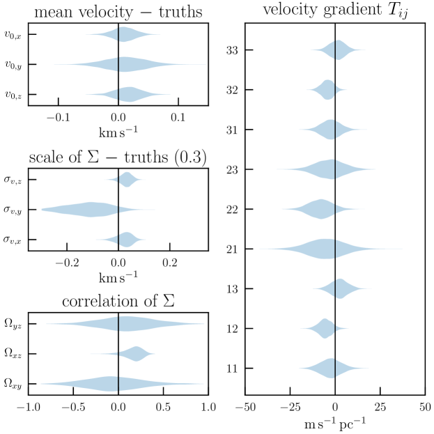
Figure 2: Model validation with mock data generated with GDR2 quality analogous to real data for the Hyades cluster. Each violin plot shows the posterior pdf of the parameter labeled on the vertical axis. We subtract the true value set to generate the mock data, thus ideally distributions should include $0$ (vertical line). The mock data in this case was generated with an isotropic velocity dispersion and no velocity gradient. All parameters here are in the ICRS coordinate system.

We implement the model in Stan, a probabilistic modelling software (Carpenter et al., 2017) using the PyStan interface. Once the generative model is specified in its own Stan language, we can either optimize using e.g., (quasi)-Newton’s methods to get a point estimate of parameters or sample the joint posterior distribution using the no-U-turn sampling (NUTS) algorithm (Hoffman & Gelman, 2011), an extension to Hamiltonian Monte Carlo (HMC) that eliminates fine-tuning of sampling parameters which can have significant effect on its sampling efficiency. HMC requires derivatives of the target density function with respect to the parameters but once tuned, can sample high-dimensional parameter spaces efficiently. Since our model is analytically differentiable with $\mathcal{O}(N)$ parameters where $N\approx 500-1000$ (number of stars), Stan and its NUTS sampling are well-suited.

In all following inferences, we sample the model parameters using NUTS with 4 chains and 2000 iterations. Discarding the first half as “warm-up” produces $4\times 1000=4000$ samples in total. We check the Gelman-Rubin statistic $\hat{R}$ of the posterior draws to ensure that the chains have converged (Gelman & Rubin, 1992; Vehtari et al., 2019).

We test our implementation using mock data of GDR2 quality generated according to the model (Section 2.1), assuming a fiducial set of parameters for the Hyades cluster. The mock data was generated using the exact GDR2 sky positions and uncertainties of the actual Hyades data which we later model (the ‘cl’ sample described in Section 3.1). We assumed the mean velocity and isotropic velocity dispersion similar to the actual values, but zero velocity gradient:

$$\begin{split}\boldsymbol{v}_{0}&=(-6.32,\,45.24,\,5.30)~{}\rm km~{}s^{-1}\\ \mathbf{\Sigma}&=0.3\mathbf{I}~{}(\rm km~{}s^{-1})^{2}\\ \mathbf{T}&=0.\end{split}$$ (11)

This is the simplest null case in which the velocity dispersion is isotropic and there is no rotation or shear. We may contrast this with our fits to the actual data to gauge the significance. We added 10% contamination from a broad background model.

The two component mixture model correctly labels cluster members and background contamination. Figure 2 shows the posterior distribution of model parameters minus their true values. Ideally, the distributions should include zero (vertical lines) meaning that we recover the true parameters put in. We find that all parameters are well recovered. The velocity dispersion along $y$-axis is biased towards a smaller value by $0.12$ $\rm km~{}s^{-1}$. There are two factors that may bias the velocity dispersion to be smaller than it is. One is if the velocity errors are too large making the internal dispersion unresolved. Another is when there is lack of information on velocity in a given direction and the prior (peaked at $0$) drives the posterior distribution. The primary reason here is likely the first as the median velocity error ($0.43$ $\rm km~{}s^{-1}$) is slightly larger the assumed dispersion. This is also why parameters involving the $y$-axis have a larger uncertainty compared to the others. Nonetheless, by incorporating partial RVs we can correctly infer null velocity gradient within $\approx 10$ $\mathrm{m}\,\mathrm{s}^{-1}\,\mathrm{pc}^{-1}$. Determining all nine components of $\mathbf{T}$ is only possible when including radial velocities available for a subset of stars, as we discussed in Section 2.1.

Section 3 Application to the Hyades cluster

We apply the method to the GDR2 data of the Hyades cluster and its tails in order to examine the internal motions in light of the improved data quality.

3.1 Data

Designation	R.A.	Decl.	$\langle P_{\mathrm{mem},i}\rangle$	fit group
Gaia DR2 49520255665123328	64.874609	21.753716	0.997003	cl
Gaia DR2 49729231594420096	60.203783	18.193881	0.996497	cl
Gaia DR2 51383893515451392	59.806965	20.428049	0.998720	cl
Gaia DR2 145373377272257664	66.061268	21.736049	0.999570	cl
Gaia DR2 145391484855481344	67.003711	21.619722	0.984320	cl

Table 2: The merged Hyades sample used for kinematic modelling. We present the first five rows and make the full table available online as supplementary material. In the full table, we add parallaxes, proper motions, radial velocities, $\mathrm{BP}-\mathrm{RP}$ colors, and $G$ magnitudes from GDR2 as well as boolean columns indicating whether the source was included the membership list of Gaia Collaboration et al. (2018b), Meingast & Alves (2019) or Röser et al. (2019). In addition to the available data, we provide the mean membership probability from our kinematic modelling.

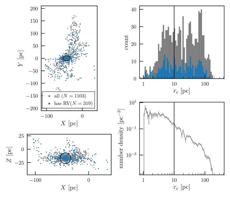
Figure 3: Distribution of the Hyades cluster sources in the merged sample. Left panels: Distribution of the Hyades cluster sources in Galactic coordinates ($X,Y,Z$) centered on the Sun. The Galactic centre is towards the right ($+X$) and the Galactic rotation is up ($+Y$). Sources with radial velocities available in GDR2 are highlighted in blue. The black circle around the cluster centre marks $10$ pc radius, dividing the ‘cl’ ($r_{c}<10$ pc) and ‘tails’ ($r_{c}>10$ pc) sample which we model separately. Right panels: Histogram and number density of Hyades sources as a function of cluster-centric distance $r_{c}$. Details are discussed in Section 3.1.

We use the cluster member selection of Gaia Collaboration et al. (2018b) as our base sample and merge this with two different samples of tidal tails by Meingast & Alves (2019) and Röser et al. (2019). The motivation for considering tidal tails is that any signature of a non-zero linear velocity field is larger at larger distances from the cluster center. In particular, shear due to Galactic tides is stronger for stars beyond the tidal radius that are farther away from the cluster potential. Both selections were made to find stars that have similar velocity with an assumed Hyades cluster mean velocity within $200$ pc distance from the Sun with some density threshold to reduce contamination by unrelated field stars having coincidentally similar velocities. However, Röser et al. (2019) made the selection from all DR2 astrometric sources (with quality cuts to clean unreliable measurements) while Meingast & Alves (2019) only selected from bright sources with their RVs measured. We exclude sources classified as “other” by Röser et al. (2019) that are significantly more spatially offset from the rest, as they are most likely not part of the Hyades cluster or its tails. In summary, there are 92 sources added from Meingast & Alves (2019) and 568 sources added from Röser et al. (2019) to the base sample.

The merged sample consists of 1103 sources and is presented in Table 2. Figure 3 shows the distribution of the sample in Galactic coordinates. Since the dynamics of stars differs within and beyond the tidal radius, we divide the sample into two based on cluster-centric distances. First, we determine the cluster centre iteratively as the mean position of stars within a radius cut using the entire sample. We start with the mean position of all stars and select stars within the chosen radius cut. We determine a new centre as the mean of those stars and repeat until the stars we select to be within the radius cut converges. The radius cut should be large enough so that the mean position is not dominated by statistical fluctuations of small number of stars, but small enough so that the increasing contamination of kinematic outliers do not affect the mean position. We choose $10$ pc as our radius cut, which is comparable to the tidal radius of the cluster. After 10 iterations, we determine the centre as the mean position of 400 stars within 10 pc: $b_{c}=(17.154,\,41.289,\,13.691)~{}{\rm pc}$ (ICRS) or $(-43.629,\,0.336,\,-16.820)$. Note that our goal here is not to determine the centre of mass of the cluster very accurately, which requires assigning mass to each star, but to come up with a reasonable reference position for the cluster centre in order to study how the kinematics of stars change with cluster-centric distance.

With the cluster centre determined, we divide the sample into two: 400 stars within $10$ pc which we call ‘cl’ and 703 stars beyond $10$ pc which we call ‘tails’. GDR2 RVs are available for 127 and 192 sources in cl and tails sample respectively. The distribution of these sources are highlighted in Figure 3 as blue circles. They are spread around in all spatial dimensions providing anchor points to break the degeneracy between perspective effect and velocity gradients. The median velocity uncertainty in R.A. and Decl. direction is $0.093$ and $0.043$ $\rm km~{}s^{-1}$ while the median radial velocity error is 0.43 $\rm km~{}s^{-1}$.

Out of concern that the velocity gradient $\mathbf{T}$ may be washed out by some small shift in the mean velocity $\boldsymbol{v}_{0}$ if left as a free parameter when modelling the tails, we fix the mean velocity to that inferred from modelling the cluster (mean of the posterior samples). We have also compared the results with when the mean velocity is still left a free parameter for tails, and found that the mean velocity inferred from tails is statistically the same as the cluster and that there are no significant discrepancies in other parameters.

3.2 Results

	cl				tails
	mean	sd	hpd 3%	hpd 97%	mean	sd	hpd 3%	hpd 97%
$f_{\mathrm{mem}}$	0.953	0.013	0.929	0.976	0.870	0.014	0.844	0.897
$v_{0,x}$ (ICRS)	-6.086	0.029	-6.144	-6.036
$v_{0,y}$ (ICRS)	45.629	0.050	45.539	45.724
$v_{0,z}$ (ICRS)	5.518	0.025	5.471	5.563
$\sigma_{x}$	0.442	0.070	0.304	0.561	0.807	0.050	0.717	0.905
$\sigma_{y}$	0.383	0.017	0.352	0.414	0.515	0.035	0.452	0.581
$\sigma_{z}$	0.371	0.056	0.270	0.470	0.389	0.017	0.359	0.421
$\Omega_{xy}$	-0.146	0.370	-0.837	0.502	0.487	0.086	0.324	0.642
$\Omega_{xz}$	-0.015	0.297	-0.561	0.536	0.197	0.061	0.081	0.312
$\Omega_{yz}$	-0.165	0.171	-0.455	0.161	0.122	0.066	0.002	0.246
$\omega_{x}$	3.270	5.513	-6.570	14.245	5.268	2.241	1.129	9.633
$\omega_{y}$	2.236	9.779	-15.803	21.091	3.613	3.256	-2.587	9.714
$\omega_{z}$	-4.440	8.713	-20.170	12.407	-6.476	1.153	-8.721	-4.342
$w_{1}$	1.447	5.461	-9.050	11.613	-2.498	2.219	-6.631	1.785
$w_{2}$	-6.589	10.074	-25.598	12.016	-2.156	3.368	-8.079	4.556
$w_{3}$	1.656	8.696	-15.204	17.449	16.897	0.916	15.250	18.724
$w_{4}$	-11.191	15.598	-41.540	18.310	4.274	2.204	0.172	8.513
$w_{5}$	10.643	6.322	-0.938	23.013	0.712	1.223	-1.529	3.037
$\kappa$	-6.500	6.417	-18.385	5.434	-5.966	1.212	-8.163	-3.650
$v_{\rm{bg},x}$ (ICRS)	-5.948	0.536	-6.927	-4.878	-5.440	1.225	-7.667	-3.073
$v_{\rm{bg},y}$ (ICRS)	46.301	0.637	45.143	47.532	37.817	1.497	35.113	40.740
$v_{\rm{bg},z}$ (ICRS)	5.421	0.524	4.485	6.441	2.217	1.244	0.002	4.752
$\sigma_{\rm bg}$	2.035	0.267	1.584	2.547	11.119	0.572	10.090	12.243

Table 3: Statistical summary of posterior distribution of parameters for cl and tails fits. For each parameter, we quote mean, standard deviation (sd), and (3, 97)% highest posterior density interval (hpd 3% and hpd 97%). Note that for the tails ($r_{c}>10$ pc) fit, $v_{0}$ is fixed to the mean of cl fit. Values are in the Galactic frame unless otherwise noted as ICRS.

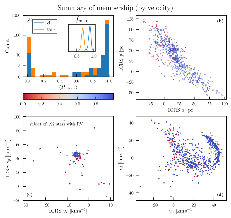
Figure 4: Summary of membership by velocity from the mixture-model fitting. Panel (a) shows the distribution of mean membership probability of individual stars for cl and tails fits (blue and orange, same as in the other figures), while the inset shows the posterior pdfs of the fraction of stars which are members, $f_{\mathrm{mem}}$. The distribution of membership probabilities is highly bimodal, i.e., there is little ambiguity in the cluster membership by velocity from these (already filtered) data. The mean membership fraction of stars for cl and tails fits are $0.95$ and $0.87$ respectively (Table 3). We show the distribution of stars for the tails coloured by their mean membership probability in three different two-dimensional projections of the data: in cartesian ICRS coordinates (b), in cartesian ICRS velocities (c); for a subset of stars with RVs (although we model all stars with astrometry) and in on-sky velocities (d). The membership here is defined only by the velocity vector.

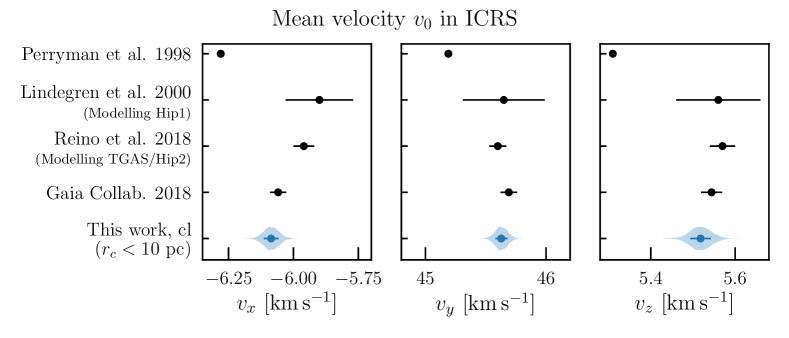
Figure 5: Mean velocity $v_{0}$ inferred from the cl fit (see Section 3.1), compared with previous studies. For this work, the shaded region (violin plot) visualizes the distribution of posterior probability density while the marker and error bars correspond to the median and (16, 84)% confidence interval (Gaussian $1\sigma$) in accordance with the other works.

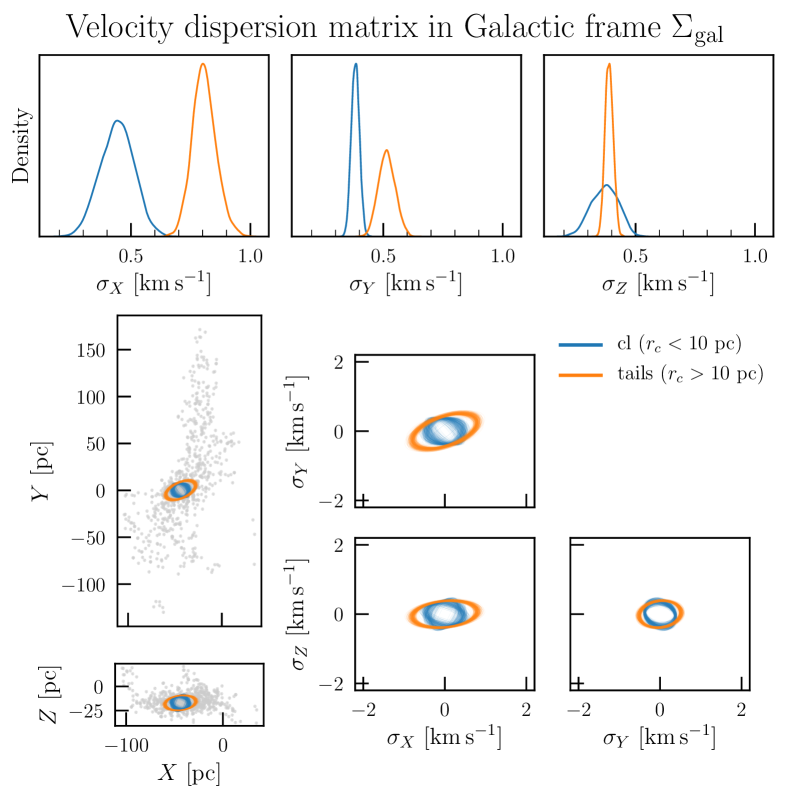
Figure 6: Velocity dispersion matrix $\Sigma_{\rm gal}$ in Galactic coordinates. The top three panels show the posterior pdf of the scale in $X$, $Y$ and $Z$ directions (with $+X$ in the direction towards the Galactic centre and $+Y$ in the direction of Galactic rotation). The bottom right corner plots visualize the $1\sigma$ dispersion ellipses projected on $2D$ planes from 400 (10%) randomly selected posterior samples. The same dispersion ellipses are plotted on top of the distribution of stars in Galactic $(X,Y)$ and $(X,Z)$ planes on the left, centered at the cluster centre.

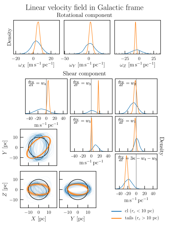
Figure 7: Decomposed linear velocity field inferred from cl and tails fits. The top row shows the rotation in the Galactic frame. The posterior pdfs for each component of the shear component of the linear velocity field (symmetric part of the tensor $T_{ij}$) is shown in the upper corner plot. On the bottom left corner plot, we visualize the shear by how it would deform a circle with radius of 10 pc in 50 Myr. The thicker line shows the mean of all posterior samples while each thin ellipse is from a hundred (25%) posterior samples randomly selected. We find negligible rotation in both cl and tails fits. On the other hand, there is significant positive shear in specific directions (in which ellipses are elongated) and negative (compressive) shear along the Galactic $Z$ direction.

We present and compare the results of cl and tails fits in the order of membership ($f_{\mathrm{mem}}$), mean velocity ($v_{0}$), velocity dispersion matrix ($\Sigma$) and linear velocity gradient ($dv_{i}/dv_{j}$), each summarized in Figures 4, 5, 6 and 7. A statistical summary of the posterior samples is provided in Table 3.

Figure 4 summarizes the membership from the simultaneous modelling of all parameters. Generally, both cl and tails have low contamination fraction and the kinematic outliers are well-separated from the members as shown in Figure 4 (a). The rest of the panels in Figure 4 show the distinction between members and non-members by the velocity mixture model in various projections of the data for tails, where each source is coloured by its mean posterior membership probability $\langle P_{\mathrm{mem},\,i}\rangle$ indicated in the colour bar: positional (b), cartesian velocity (c) and projected velocity (d) space. Naturally the distinction is most clear cut in cartesian velocity space (c) but note that while we can only put stars with RVs on this diagram, the rest of the data without RVs are consistently and simultaneously modelled and shown in (b) and (d). In projected velocities, stars with the same velocity can exhibit a non-trivial trajectory due to changing perspective (d). Most importantly, this nuisance, i.e., the existence of kinematic outliers, is marginalized out in our inference of internal kinematics, making the results robust to contamination in member selection. We make the (kinematic) membership probability from our analysis available (Table 2), as this may be useful for other applications.

Figure 5 shows the inferred mean velocity $v_{0}$ of the cluster in ICRS coordinates when modelling the cluster proper (cl) in comparison with a number of previous studies. We find our estimate for the mean velocity to be consistent with Gaia Collaboration et al. (2018b), which is also from the GDR2 data, as well as previous studies modelling the TGAS and Hipparcos data (Reino et al., 2018; Lindegren et al., 2000). The main difference is that the uncertainties are smaller, thanks to better quality and larger size of GDR2 data.

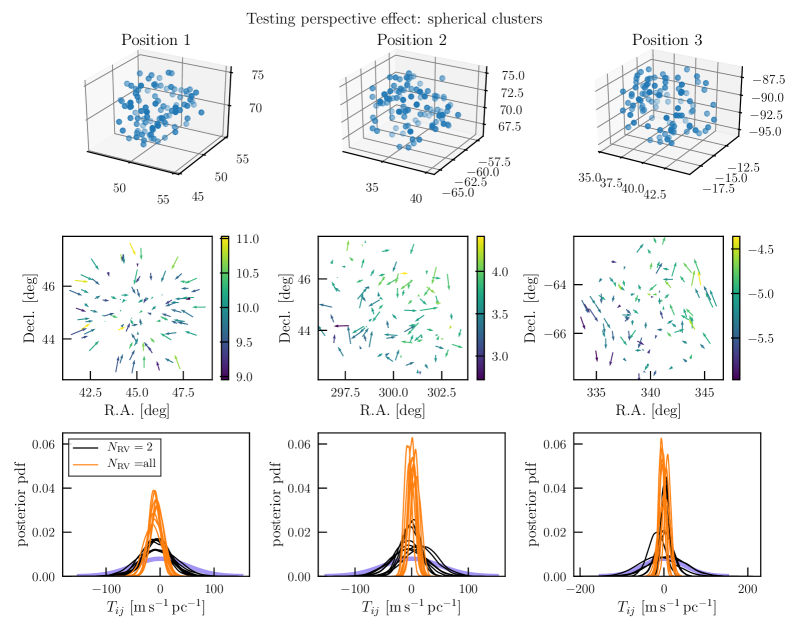
Figure 14: Fitting mock spherical clusters at the three positions shown in Figure 12. For details of what each panel shows, see the caption of Figure 13. The residual proper motion patterns are more messy in these cases as they are also affected by each star’s distance, unlike grid sheet clusters where all stars are at $100$ pc.

In previous kinematic modelling of the Hyades, the velocity dispersion was assumed to be isotropic. Moreover, the larger noise in proper motions and parallaxes and the lack of RVs meant that the small internal dispersion is only marginally resolved. With GDR2 and a more flexible model, we find that the velocity dispersion is indeed mildly anisotropic for the cluster (cl ($r_{c}<10$), Figure 6). However, the velocity ellipsoid of the tails is strongly anisotropic and elongated in the Galactic radial direction, while remaining unchanged in Galactic vertical direction. Hints of this velocity dispersion anisotropy can be already seen with TGAS data (Reino et al., 2018, Figure 14); it is most clear from the bottom row of their figure where the velocities are calculated using the kinematically-improved parallaxes from their kinematic modelling and is largely consistent with what we find, although modelling is required to deconvolve the noise and covariance from the apparent dispersion.

In reality, the velocity dispersion likely changes with the cluster-centric distance. Generally, the velocity dispersion decreases with radius, but may deviate from the expectation of isolated bound cluster starting at $\approx$ half tidal radius. This is because, under the influence of the tidal field, a population of stars that are energetically unbound yet still within the tidal radius (“potential escapers”) may increasingly dominate the kinematics of a cluster (e.g., Baumgardt, 2001; Küpper et al., 2010). Figure 12 of Baumgardt (2001) indicates that the fraction of potential escapers may be $\approx 20\%$ for the Hyades. Beyond the tidal radius, the velocity dispersion of the tidal debris increases with radius. While we do not model the velocity dispersion as a function of cluster-centric radius, the increase of the inferred velocity dispersion in the Galactic radial and azimuthal directions for the tails compared to the cluster is consistent with this expectation (see also Meingast & Alves, 2019; Ernst et al., 2011). On the other hand, the velocity dispersion in the Galactic vertical direction remains almost unchanged.

Finally, the posterior probability distribution of the linear velocity field parameters are presented in Figure 7. We transform the velocity gradient tensor to more physically interpretable components, namely rotation and shear. We do not find any significant rotation in both fits. For the cluster (cl, $r_{c}<10$ pc), there is no net expansion or contraction but there is $\approx 2\sigma$ level shear signals that the cluster is being stretched in the Galactic rotational direction ($Y$ axis) and compressed in the Galactic vertical direction ($Z$ axis). A similar shear field is much more significantly detected in tidal tails and its direction is more well-defined.

3.3 Discussion

3.3.1 Effects of Gaia Frame Rotation for Bright Sources

The proper motions of bright sources ($G\lesssim 13$) in GDR2 have a systematic residual reference frame rotation of $\approx 0.15$ ${\mathrm{mas}\,\mathrm{yr}^{-1}}$, whereas faint sources do not show any significant spin relative to quasars (Lindegren et al., 2018). Because the cluster and its tails are spread over a large area on the sky, this could potentially inject a fake linear velocity field signal. We tested for any effect this might have on the inference by comparing each fit with and without the correction for bright sources. We apply the correction for rotation provided by Lindegren to sources brighter than $G=12$. We found that for the Hyades, the systematic Gaia frame rotation for bright sources has negligible effect on all parameters.

3.3.2 Comparison to HARPS study by Leão et al. (2019)

Recently, Leão et al. (2019) compared spectroscopic RVs measured from High-Accuracy Radial velocity Planet Searcher (HARPS) spectra with the astrometric RVs for 71 stars in the Hyades cluster. They found that the RV difference is skewed and dependent on the positions of the stars on sky. They attributed this to cluster rotation of $42.3\pm 4.0$ $\mathrm{m}\,\mathrm{s}^{-1}\,\mathrm{pc}^{-1}$. We first note that rotation of such magnitude would easily be revealed by the current method and data. However, our modelling of GDR2 astrometry and partial RVs suggests that there is no significant rotation (Figure 7) in the cluster. The strongest signal we find in the linear velocity gradient is that of positive shear along the Galactic radial direction. We find that the inferred shear without any rotation can also produce the $\Delta RV$ versus right ascensions trend seen by Leão et al. (2019).

3.3.3 Effects of Binarity and Spurious Astrometry

Binary stars tend to bias the velocity dispersion determined from (single-epoch) spectroscopic RVs to a larger value as they may include jitters due to binary orbital motion on top of intrinsic dispersion. However, it is important to note that the RVs and RV errors reported in GDR2 are not from a single-epoch measurement, but the median and scatter around the mean of multiple per-transit RV measurements for each source (Katz et al., 2019). Thus, binarity makes the GDR2 RV errors larger, which will bias the velocity dispersion to a smaller value (Section 2.2) in opposite to the usual expectation . Larger errors also mean that those stars will not drive the fit as data are weighted by $(1/\mathrm{error}^{2})$. Of course, if the binary orbital motion introduces a large enough shift in RV, the star may be excluded from the cluster entirely by the mixture model.

We have tested how much the inferred velocity dispersion is affected by spurious astrometric measurements including those caused by astrometric binaries by removing the top $\approx 10$% outliers in re-normalized unit weight error (RUWE), i.e., 54 out of 400 sources in the cl sample with $\mathrm{RUWE}>1.396$. The RUWE is a goodness-of-fit metric for the single-source astrometric model re-normalized in order to take out the colour and magnitude dependent systematics present in GDR2. Because one main astrophysical cause that makes a source deviate from the single-source model is binarity, it can be used to pick out candidate binaries with astrometric wobble (Belokurov et al., 2020). It is also the preferred metric to filter out ill-behaved astrometric sources (Lindegren et al., 2018) . We find that the velocity dispersion remains the same and is not driven by potential astrometric binaries or spurious astrometric measurements.

Based on these considerations, we conclude that binarity or spurious astrometry are unlikely to significantly bias the velocity dispersions. We note that our velocity dispersion estimate of the cluster (the cl sample) is compatible with the isotropic dispersion determined in previous studies using different methods and data (Reino et al., 2018; Lindegren et al., 2000, $\sigma_{\mathrm{1D}}\approx 0.3~{}\rm km~{}s^{-1}$),

3.3.4 Effects of underestimated errors

A bug in the astrometric processing software (“DOF bug”, Lindegren et al., 2018) resulted in serious underestimation of GDR2 astrometric uncertainties. While it has been corrected ad hoc at a later stage of the processing, validation with external data show that they are still underestimated (Gaia Collaboration et al., 2018a; Arenou et al., 2018). The degree of underestimation depends on source magnitudes and varies from 10% to 50%. In an independent investigation, Brandt (2018) found a similar conclusion: cross-calibrating GDR2 with Hipparcos they find a global multiplicative error inflation factor of $1.743$ for the proper motions. Moreover, they find that how much the reported errors are underestimated is spatially varying.

Inference of internal dispersion is degenerate with and dependent upon correct observational uncertainty estimates, as both work to add noise to the proper motions except the former is intrinsic to the cluster. This, combined with binaries and spurious astrometric sources, may bias the inferred velocity dispersion high. We tested whether the velocity dispersion changes when we account for both simultaneously by first removing top 10% RUWE outliers (Section 3.3.3) and then inflating the errors of parallaxes and proper motions for all sources by a factor of 2. Even in this rather extreme scenario of error underestimation, we find no significant difference in our inference of the internal velocity dispersion. GDR2 astrometry for these nearby stars are precise enough to resolve $\approx 0.4$ $\rm km~{}s^{-1}$ internal dispersion (see also Figure 9).

Section 4 The Present and Future of the Hyades

We now discuss our kinematic results with a view to assessing the present status and future prospects of the Hyades cluster and tails.

4.1 Steady-state Dynamical Models

First, let us build a steady-state dynamical model of the Hyades cluster, inspired by the observation that the light profile in the inner parts follows a Plummer model (Gunn et al., 1988; Röser et al., 2011). It has long been known that the shape of the Hyades is flattened along the Galactic $Y$ and $Z$-directions and elongated along the $X$-direction toward the Galactic Centre (Figure 3; Oort, 1979; Perryman et al., 1998; Röser et al., 2011). This is consistent with the effect of the Galactic tides. Using Reino et al. (2018), the Hyades has a prolate shape with axis ratio $q\approx 0.8$ at the tidal radius of $r_{\rm t}\approx 10$ pc. This suggests a model with potential

$$\phi(x,y,z)=-{GM\over\Bigl{(}(a^{2}+r_{\rm c}^{2})^{2}+2b^{2}(y^{2}+z^{2})\Bigr{)}^{1/4}}.$$ (12)

Here, ($x,y,z$) are cluster-centric analogues of the Sun-centred $(X,Y,Z)$ coordinates, whereas $r_{\rm c}^{2}=x^{2}+y^{2}+z^{2}$. When $b=0$, this is recognised as the familiar Plummer (1911) sphere. We use Poisson’s equation to obtain the density $\rho(x,y,z)$. For $b\neq 0$, it corresponds to a prolate Plummer spheroid with a long axis in the $x$-direction and two short axes in $y$ and $z$. Using the result from Röser et al. (2011), we set the Plummer scale length $a$ as 3.1 pc and choose the total mass $M$ so that the central density is 2.21 $M_{\odot}$ pc^-3. The axis ratio at the tidal radius is

$$q=2^{1/4}(5a)^{5/2}{300a^{4}+164a^{2}b^{2}-9b^{4}\over(3a^{2}+2b^{2})(50a^{2}+9b^{2})^{9/4}}$$ (13)

So, the scale length $b$ is taken as $2.08$ pc to yield the desired axis ratio of the density contours as $q\approx 0.8$ at the tidal radius (Reino et al., 2018). This gives us a good representation of the Hyades stellar density within $r_{\rm t}=10$ pc.

It is now simple to solve the (steady-state) Jeans equations which relate the velocity dispersions to the gravity field of the cluster. As the dispersion tensor of the cl sample is close to alignment in the ($x,y,z$) coordinates (see Table 3 and Figure 7), we set the cross-terms to zero at outset, so the three Jeans equations simplify to

$${\partial\rho\sigma^{2}_{x_{i}}\over\partial{x_{i}}}=-\rho{\partial\phi\over\partial x_{i}},\qquad\qquad x_{i}=(x,y,z).$$ (14)

The position-dependent velocity dispersions are then mass-weighted within the tidal radius to obtain ($\sigma_{x},\,\sigma_{y},\,\sigma_{z}$) = ($0.183,\,0.173,\,0.173)$ $\rm km~{}s^{-1}$. These can be compared with the numbers in Table 3.

The velocity anisotropy of the dynamical model $\sigma_{x}/\sigma_{y}$ is 1.06. From the fitting of the cl sample ($r_{c}<10$ pc), we infer $\sigma_{x}/\sigma_{y}=1.2^{+0.20}_{-0.22}$. Thus, while it is of mild significance mainly due to the lack of high-precision RVs for the bulk of the sample, the slight elongation of the velocity ellipsoid along $x$-axis is consistent with the dynamical model. The flattening of the cluster can be explained by the velocity anisotropy observed and does not require rotation, which is not detected. However, the total three dimensional velocity dispersion of the dynamical model is 0.305 $\rm km~{}s^{-1}$(mass-weighted over the cluster within the tidal radius). This is a factor of $\approx 2$ smaller than the inferred total three dimensional velocity dispersion from the kinematical analysis, $\sqrt{\sigma^{2}_{x}+\sigma^{2}_{y}+\sigma^{2}_{z}}=0.692$ $\rm km~{}s^{-1}$ (Table 3), leading to a factor of $\approx 4$ discrepancy in total mass. In fact, using the measured dispersions, our model suggests a mass of the Hyades within its tidal radius of $900^{+250}_{-220}{\rm M}_{\odot}$.

It is instructive to compare these results with Röser et al. (2011), especially their Table 3. Their three-dimensional velocity dispersion for stars within the tidal radius is $0.77\pm 0.10$ $\rm km~{}s^{-1}$, in agreement with the results in Table 3. For a theoretical prediction, they find $0.36$ $\rm km~{}s^{-1}$using the virial equation, essentially a cruder form of the Jeans equations used here. So, they also find a discrepancy by a factor of $\approx 2$ between observations and steady-state models. They ascribe the disparity mainly to possible inflation of the dispersion caused by binaries while some hidden mass in white dwarfs, low mass stars, and binary companions may increase the observed mass by less than 50%. However, we argued in Section 3.3.3 that the velocity dispersion we determine is not significantly biased due to binarity. We conclude that the measured velocity dispersions of the Hyades stars – even within the tidal radius ($\approx 10$ pc) – are much too high. This must be caused by a dynamical mechanism completely absent from a steady-state Jeans modelling. By extension, the Hyades cluster cannot possibly be in virial equilibrium and must be close to its disruption.

If a cluster is in a perfectly circular orbit in an axisymmetric potential, the gravitational potential in the frame co-rotating with the cluster is static and tidal heading would be irrelevant. Such conditions are never met in reality. The epicyclic motion of the cluster introduces time-variation, which results in tidal heating. While repeated tidal shocks due to encounters with molecular clouds may also heat the cluster, the preferential direction in which the velocity dispersion is larger in both cl an tails fits naturally seem to prefer the Galactic tides as the explanation. Once stars escape from the cluster beyond the tidal radius of $\approx 10$ pc for the Hyades, the escaped stars follow their own epicyclic motions. This, combined with the fact that tidal heating is even more effective for the stars in the tails that are free from the cluster potential, may explain the even larger velocity dispersion along the $x$-direction for the tails fits.

4.2 Evolving Models

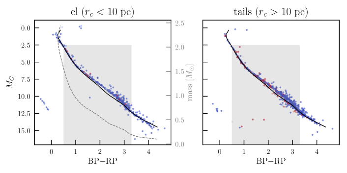
Figure 8: Color-magnitude diagrams of the cluster and tails. Sources are colored by their mean membership probability as in Figure 4. In order to estimate $\eta_{\rm now}$, we convert the $\mathrm{BP}-\mathrm{RP}$ color to mass using the MIST isochrone (Choi et al., 2016) of 680 Myr and $\text{[Fe/H]}=0.24$ (Gossage et al., 2018). The isochrone in the color-magnitude space is the black line in each panel. The color-mass relation is shown in the left panel as the gray dashed line with the corresponding y-axis on the right. Only sources within the shaded region ($0.5<\mathrm{BP}-\mathrm{RP}<3.3$ corresponding to $0.19<m<1.56$ $M_{\odot}$) are considered (see Section 4.2).

To build evolving models of the Hyades, we assume that the tidally-stripped stars leave with nearly zero energy. Then, the mass $M(t)$ and Plummer scale length $a(t)$ of the cluster decline with time, while the cluster energy $E$

$$E=-{3\pi\over 64}{GM^{2}(t)\over a(t)}.$$ (15)

remains constant. As Küpper et al. (2008) point out, this is a surprisingly good approximation as stars cross the tidal radius with almost zero velocity.

We assume that mass is lost according to (cf Hénon, 1961; Gnedin et al., 1999)

$${dM\over dt}=-{kM\over t_{\rm r}}$$ (16)

where $k$ is an unknown constant and $t_{\rm r}$ is the relaxation time at the half-mass radius (see e.g., Spitzer & Hart, 1971), which for the Plummer model is

$$t_{\rm r}=0.206{M(t)^{1/2}a(t)^{3/2}\over G^{1/2}\langle m_{\star}\rangle\log\Lambda}.$$ (17)

Here, $\langle m_{\star}\rangle$ is the mean stellar mass, while $\Lambda$ is the Coulomb logarithm. This ansatz (16) encodes the complicated physics of evaporation and ejection of stars, tidal stripping and disc shocking. Although simple, it has been used with success to represent the results of full N-body simulations of globular clusters, with values of $k$ in the range 0.05 - 0.007 (e.g., Spitzer & Chevalier, 1973; Gnedin et al., 1999).

This differential equation (16) can be solved (Binney & Tremaine, 2008, chap 7) to give power-law solutions for the mass of the cluster $M(t)$, its scale length $a(t)$ and its tidal radius $r_{\rm t}(t)$. Specifically, we obtain:

$$M(t)=M_{0}\left(1-{7kt\over 2t_{r,0}}\right)^{2/7},\qquad a(t)=a_{0}\left(1-{7kt\over 2t_{r,0}}\right)^{4/7},$$ (18)

where $t$ is the time since formation, whilst a zero subscript indicates the value at the initial time.

The age of the Hyades cluster is $t_{\rm now}\approx 680$ Myr (Gossage et al., 2018). Its present day stellar mass is $M(t_{\rm now})=M_{\rm now}\approx 300$ $M_{\odot}$, whilst its relaxation time $t_{\rm r,now}$ is $\approx 60$ Myr. By themselves, these data are not enough to prescribe the location of the Hyades on the evolutionary tracks given by eqs (18). However, there is a further piece of information that is susceptible to observational scrutiny, namely the ratio of the stellar mass in the tails to the mass in the cluster

$$\eta(t)={M_{0}-M(t)\over M(t)}.$$ (19)

Although this is not precisely known, it is evident that the tails are mature and well-developed (see Figure 3).

In order to estimate $\eta_{\rm now}$ from the data, we use the MIST model isochrone (Choi et al., 2016) of 680 Myr and $\text{[Fe/H]}=0.24$ (Gossage et al., 2018) to convert $\mathrm{BP}-\mathrm{RP}$ color to mass. Figure 8 shows the distribution of sources for the cluster and tails along with the model isochrone. The color-mass conversion curve is also shown in the gray dashed line in the left panel. We only consider stars within the color range $0.5<\mathrm{BP}-\mathrm{RP}<3.3$ indicated as the shaded gray region in Figure 8. This corresponds to $0.19<m<1.56$ $M_{\odot}$ in mass. The blue limit is set so as not to deal with the main-sequence turn off, which makes color-mass relation non-monotonic. At the red color limit, the observed magnitude is $G\approx 15-16$, well below the Gaia magnitude limit ($G\approx 20$). When summing up the mass of stars, we only include stars with mean membership probability larger than $0.5$ taking advantage of the kinematic membership we infer in our kinematic modelling. We find that the cluster and tails contain $157$ ${\rm M}_{\odot}$ (288 sources) and $239$ ${\rm M}_{\odot}$ (587 sources) respectively at this color (mass) range, resulting in our crude $\eta_{\rm now}$ estimate as $\eta_{\rm now}\gtrsim 1.5$. This is likely a lower bound as the extent of tails discovered and included in our study is not complete. Note also that the model isochrone is not well matched to the data at low mass and that we have not taken binarity of sources into account in converting color to mass. A more careful modelling is required to refine individual sources’ mass estimate.

In any case, the Hyades has already undergone substantial destruction as $\eta_{\rm now}$ is evidently larger than 1. The original mass of the Hyades cluster at birth is

$$M_{0}=M_{\rm now}(1+\eta_{\rm now})\gtrsim 750~{}{\rm M}_{\odot}.$$ (20)

By using $\eta$ as a proxy for time, we find the present day mass loss rate of stars is

$$-{dM\over dt} ={2((1+\eta_{\rm now})^{7/2}-1)\over 7}{M_{\rm now}t_{\rm r,now}\over t_{\rm now}^{2}}$$ (21)

$$\gtrsim 0.26~{}{\rm M}_{\odot}\,{\rm Myr}^{-1}.$$

These results can be compared with the numerical simulations of Ernst et al. (2011), who attempted to reproduce the present-day cumulative mass profile, stellar mass and luminosity function of the Hyades. Their best-fitting Plummer model has an initial mass of $1230\,M_{\odot}$ and an average mass loss rate of $1.4\,M_{\odot}$Myr^-1.

The mass loss rate will increase rapidly as the cluster approaches complete disintegration. The lifetime of the Hyades is

$$t_{\rm life}=t_{\rm now}\left({1\over 1-(1+\eta_{\rm now})^{-7/2}}\right)\lesssim 709~{}{\rm Myr}$$ (22)

As the age of the Hyades is $\approx 680$ Myr, the cluster is in its death throes. The final dissolution will take place over the next $\lesssim 30$ Myr. The end is nigh for the Hyades irrespective of the precise value of $\eta_{\rm now}$, providing it is $\gtrsim 1$. This is because all such curves (22) decline precipitously at late times and the bound mass drops quickly to zero. At dissolution, the stars of the Hyades are all unbound, but they have not necessarily dispersed from the location of the object. Of course, as the tails continue to stretch and evolve, the stars disperse and the remnant itself becomes indistinguishable from the tails (cf the dissolution of Ursa Major II discussed in Fellhauer et al. (2007), especially their Figure 6).

Note that both our steady-state and evolving models tell a consistent story. The Hyades cluster is far from any virial equilibrium, and it cannot be expected to survive in it present fragile state for much longer. This result is implicit in earlier work (Röser et al., 2011; Ernst et al., 2011), but the phenomenal quality of the Gaia proper motions allow us to be much more explicit here.

4.3 The Hyades Tails

The planar velocity field in the tails relative to the systemic motion of the cluster can be described in terms of analogues of the Oort Constants as (Oort, 1928; Ogrodnikoff, 1932; Milne, 1935; Murray, 1983)

$$\mathbf{T_{2}}=\left(\begin{array}[]{c@{\;\;}c}\partial v_{x}/\partial x&\partial v_{y}/\partial x\\ \partial v_{x}/\partial y&\partial v_{y}/\partial y\end{array}\right)\equiv\left(\begin{array}[]{c@{\;\;}c}K+C&A-B\\ A+B&K-C\end{array}\right).$$ (23)

The parameters $A$, $B$, $C$, and $K$ are the Oort Constants and they measure the local (two-dimensional) divergence ($K$), vorticity ($B$), azimuthal ($A$) and radial ($C$) shear of the velocity field. By comparison with Table 3, we see that

$$A =w_{3}=16.90\pm 0.92\,\mathrm{m}\,\mathrm{s}^{-1}\,\mathrm{pc}^{-1},$$

$$B =\omega_{z}=-6.48\pm 1.15\,\mathrm{m}\,\mathrm{s}^{-1}\,\mathrm{pc}^{-1},$$ (24)

$$C =\frac{1}{2}(w_{4}-w_{5})=1.78\pm 1.27\,\mathrm{m}\,\mathrm{s}^{-1}\,\mathrm{pc}^{-1}$$

$$K =\frac{1}{2}(w_{4}+w_{5})=2.49\pm 1.27\,\mathrm{m}\,\mathrm{s}^{-1}\,\mathrm{pc}^{-1}$$ (25)

These may be compared to the Oort constants describing deviations of the velocity field from the Local Standard of Rest. Using the TGAS catalogue, Bovy (2017) found: $A=15.3\pm 0.4$ $\mathrm{m}\,\mathrm{s}^{-1}\,\mathrm{pc}^{-1}$, $B=-11.9\pm 0.4$ $\mathrm{m}\,\mathrm{s}^{-1}\,\mathrm{pc}^{-1}$, $C=-3.2\pm 0.4$ $\mathrm{m}\,\mathrm{s}^{-1}\,\mathrm{pc}^{-1}$and $K=-3.3\pm 0.6$ $\mathrm{m}\,\mathrm{s}^{-1}\,\mathrm{pc}^{-1}$. Exact agreement is not expected, as (i) the Taylor expansion is around the mildly eccentric Hyades orbit rather than a cold circular orbit in the Galactic plane ($Z=0$), (ii) processes like the mass loss, disk and bulge shocking and perturbations by molecular clouds and spiral arms may also affect the kinematics of the tidal tails.

Using Table 3, the velocity dispersion of tail material has $\sigma_{y}/\sigma_{x}=0.64\pm 0.06$ and $\sigma_{z}/\sigma_{x}=0.48\pm 0.04$. These results may be compared to the analogous values for the thin disk ($\sigma_{y}/\sigma_{x}=0.70\pm 0.13$ and $\sigma_{z}/\sigma_{x}=0.64\pm 0.008$) and the thick disc ($\sigma_{y}/\sigma_{x}=0.67\pm 0.11$ and $\sigma_{z}/\sigma_{x}=0.66\pm 0.11$) found with Gaia DR1 by Anguiano et al. (2018). Note that steady-state populations in an axisymmetric disc with a flat rotation curve are predicted to have $\sigma_{y}/\sigma_{x}=\sqrt{2}=0.707$ in epicyclic theory (e.g., Evans & Collett, 1993; Kuijken & Tremaine, 1994), very close to what is seen for the thin disc. The Hyades tail stars possess kinematics distinct from both discs with the in-plane dispersion ratio comparable to the thick disc, but the vertical ratio much colder. The vertex deviation $\ell_{uv}$ and tilt angle $\ell_{uw}$ are defined as (e.g., Smith et al., 2012)

$$\ell_{uv}={1\over 2}\arctan\left({2\Omega_{xy}\over\sigma^{2}_{x}-\sigma^{2}_{y}}\right),\quad\ell_{uw}={1\over 2}\arctan\left({2\Omega_{xz}\over\sigma^{2}_{x}-\sigma^{2}_{z}}\right),$$ (26)

Both angles should vanish for a relaxed stellar population in an axisymmetric disc (e.g., Smith et al., 2009). However, the values of the cross terms in Table 3 betray significant vertex deviation and tilt for the Hyades tail population, and we calculate $\ell_{uv}=34^{\circ}$ and $\ell_{uw}=19^{\circ}$. These are very different from the thick disc, which has a roughly constant vertex deviation of $\ell_{uv}\approx-15^{\circ}$ and tilt $\ell_{uw}\approx-10^{\circ}$. They are however similar to the vertex and tilt of the thin disc stars with comparable metallicity ([Fe/H] $\approx 0.24$), as shown in Figures 11 and 12 of Anguiano et al. (2018). Nonetheless, the axis ratios and misalignment angles together demonstrate that the kinematic properties of the tail material do differ from those of the field population, which may enable efficient filtering of tail stars to aid detection of material at larger distances from the cluster.

Section 5 Summary

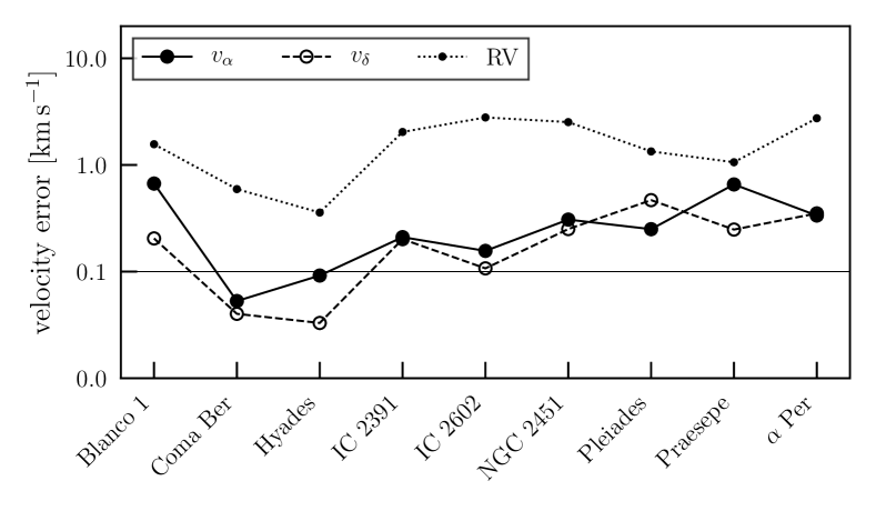
Figure 9: Median GDR2 velocity errors for a number of nearby open clusters and associations (Gaia Collaboration et al., 2018b).

The unprecedented quality of the Gaia data and its synergy with various spectroscopic surveys have already started to improve dramatically our understanding of star clusters. Internal kinematics of clusters in particular can provide valuable hints as to their formation, evolution and destruction.

We presented a method to model the internal kinematics of stars in a cluster or association, which builds upon and extends previous works with Hipparcos and Gaia. Our model allows for anisotropic velocity dispersions and a linear velocity gradient (equivalently, rotation and shear). It incorporates radial velocity measurements for a subset of stars with astrometry, and accounts for contamination by background sources (in terms of velocity) via a mixture model. We implemented the method in a modern statistical modelling language and validated the implementation with mock data generated with similar quality as GDR2.

We applied the method to the GDR2 data of the Hyades cluster and its tails, which have recently been discovered using the same data (Meingast & Alves, 2019; Röser et al., 2019). We divided the sample into two, the cluster proper (cl, $r_{c}<10$ pc) and the tidal tails (tails, $r_{c}>10$ pc).

While the velocity dispersion of the cluster is nearly isotropic, there is slight elongation of the velocity ellipsoid in the Galactic radial direction consistent with what is expected from the prolate shape of the cluster. The Hyades shows no evidence for internal rotation. Strictly speaking, this result is restricted to solid body rotation and other rotation laws are possible for clusters (e.g., Ernst et al., 2007; Jeffreson et al., 2017), though in the cluster centre they do reduce to solid body rotation. There is almost no net expansion or contraction of the cluster stars, but there are measurable ($\approx 2\sigma$) negative and positive gradients in $dv_{y}/dy$ and $dv_{z}/dz$ respectively. The shear without any rotation can produce the trends seen by Leão et al. (2019) and claimed as rotation.

The stars in the tidal tails ($r_{c}>10$ pc) show clear velocity dispersion anisotropy and linear velocity gradient. The kinematics of the tail stars parallel to the Galactic plane can be decomposed into a shear of $16.90\pm 0.92$ $\mathrm{m}\,\mathrm{s}^{-1}\,\mathrm{pc}^{-1}$and a vorticity of $-6.48\pm 1.15$ $\mathrm{m}\,\mathrm{s}^{-1}\,\mathrm{pc}^{-1}$. These values are different from the local Oort constants of $A=15.3\pm 0.4$ $\mathrm{m}\,\mathrm{s}^{-1}\,\mathrm{pc}^{-1}$and $B=-11.9\pm 0.4$ $\mathrm{m}\,\mathrm{s}^{-1}\,\mathrm{pc}^{-1}$ (Bovy, 2017). This is because the velocity gradients are measured with respect to the Hyades cluster orbit, which is mildly elliptical with an eccentricity of $\approx 0.1$ and a vertical libration amplitude of $\approx\pm 70$ pc  (Ernst et al., 2011). The classical Oort constants apply in the cold limit of vanishing random motions, in which the mean streaming velocity is the velocity of closed circular orbits supported by the Galactic potential.

The Hyades cluster has a prolate shape, fashioned by the Galactic tides. It is flattened along the $y$ and $z$-directions, but elongated along the $x$-direction towards the Galactic centre. The stellar density of the cluster is well modelled by a prolate Plummer spheroid. By solving the Jeans equations, we find the velocity dispersions needed to support the cluster in virial equilibrium. These are a factor of $\approx 2$ smaller than the values inferred from our kinematic analysis. It follows that the Hyades cluster is not in virial equilibrium. Many of the stars in our cl sample are unbound. Their velocities are strongly enhanced by tidal heating, providing the population of “potential escapers” identified by Baumgardt (2001) and Küpper et al. (2010).

Simple models of Hyades evolution driven by mass loss are then developed. Assuming the stripped stars leave with almost zero energy with respect to the cluster, the total mass and tidal radius behave like power-laws of the time until dissolution. Given an estimate of the ratio of the mass in the tails to the mass in the cluster at the present epoch, then the original mass, the current mass loss and the time till disruption can be computed. Using the extent of tidal tails so far discovered, we can place a lower bound on the initial mass of the Hyades at birth and its current mass loss rate as $M_{0}\gtrsim 750~{}{\rm M}_{\odot}$ and $-dM/dt\gtrsim 0.26{\rm M}_{\odot}\,\mathrm{Myr}^{-1}$. We estimate that less than $30$ Myr is left until the final dissolution; the Hyades is in its death throes.

There are a number of avenues for future exploration. Although our kinematic model has a global velocity dispersion matrix for the cluster, in practice it changes as a function of distance from the cluster centre. For example, in Plummer models of the Hyades, the velocity dispersions fall by a factor of 1/3 on moving from the centre to the tidal radius. Thus, a better kinematic model might be one in which the dispersion matrix changes as a function of cluster-centric distance. As this introduces more free parameters, it inevitably increases the uncertainties on inferred parameters.

Secondly, much remains to be done to complete the census of Hyades tail members as the searches so far have been limited to 200 pc from the Sun (Röser et al., 2019; Meingast & Alves, 2019). We can use the shear to estimate the total length of the tidal tails of the Hyades. Given its age of $t_{\rm now}\approx 680$ Myr, then the first stars to stripped will now lag or lead the cluster by a distance

$$L\approx 2A\,{\sqrt{3}r_{\rm t}}\,t_{\rm now}\approx 400\,{\rm pc},$$ (27)

where we have taken the Oort constant $A$ for the tails from eq (4.3) and assumed the tails are displaced in radius from the cluster by $\sqrt{3}r_{\rm t}$ using eq. (17) of Just et al. (2009). The simulations of Ernst et al. (2011) found a somewhat larger value of $L\approx 800$ pc. Of course, it becomes increasingly challenging to trace convincingly the low-density tidal tails as the distance from the cluster centre increases.

The most favourable locations at which to look for extensions of the Hyades tails are the overdensities caused by epicyclic bunching of tail stars (Küpper et al., 2008; Just et al., 2009). Once stars leave the Hyades, their motion is well-described by epicyclic theory. The relative velocity of tail stars is then smallest at the pericentres of the epicycles. The locations of epicyclic clumpings are (Just et al., 2009)

$$y\approx\pm{4\pi\Omega\over\kappa}{4\Omega^{2}-\kappa^{2}\over\kappa^{2}}\sqrt{3}r_{\rm t}$$ (28)

where $\Omega$ and $\kappa$ are the circular and epicyclic frequencies. For the Hyades, this gives $y\approx\pm 154$ pc, taking $\kappa/\Omega=\sqrt{2}$ appropriate for a flat rotation curve. This clumping phenomenon has only been seen in simulations (Küpper et al., 2008; Just et al., 2009), but has not been unambiguously shown to occur in nature. In fact, perturbations from spiral arms or giant molecular clouds may complicate the picture from epicyclic theory and disperse such density enhancements, rendering them undetectable in practice.

Finally, although we have concentrated on the Hyades cluster in this paper, it is natural to extend the work to other nearby open clusters with high quality data. Figure 9 shows median velocity errors derived from GDR2 spectroscopic and astrometric measurements for a sample of nearby open clusters (Gaia Collaboration et al., 2018b). In terms of precision of the velocities, the Hyades is the most propitious target, with Coma Berenices, IC 2602 and Praesepe being the next most favourable. The number of members in GDR2 varies from $\approx 150$ for Coma Berenices (Tang et al., 2018) to $\approx$ 1500 for the Pleiades (Gao, 2019). Some of these open clusters also have newly identified tails (Röser & Schilbach, 2019; Tang et al., 2019). This opens up the possibility of using the tails of nearby open clusters to measure kinematic properties at multiple locations in the Galaxy.

The data underlying this article are available in the article and in its online supplementary material. The modelling code is available at http://github.com/smoh/kinesis.

Appendix A Perspective effect

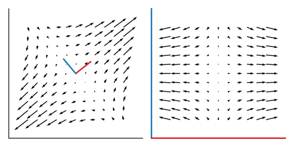
Figure 10: Shear is expansion rotated. The shear is the symmetric part of the velocity gradient matrix and so can be diagonalised in a suitably chosen frame in which the motion appears as expansion or contraction along the axes.

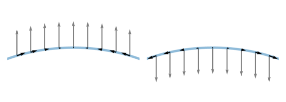
Figure 11: Receding clusters appear to be contracting while approaching clusters appear to be expanding. The blue circle is the celestial sphere.

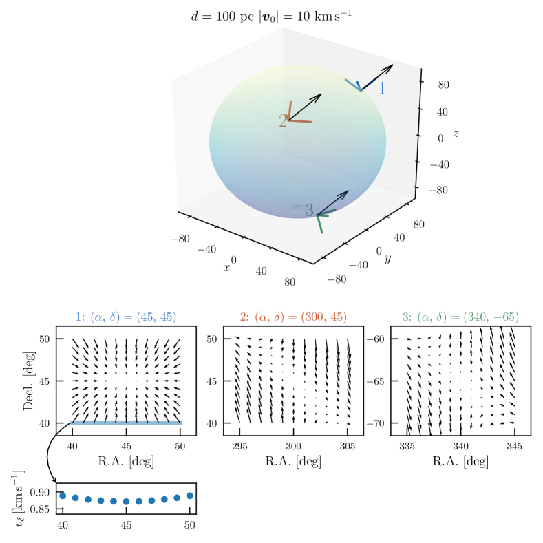
Figure 12: Perspective effect of the same mean velocity vector $\boldsymbol{v}_{0}^{T}=(v_{x},\,v_{y},\,v_{z})=(5.0,5.0,7.071)~{}\rm km~{}s^{-1}$ at three different sky positions. The top 3D plot shows the mean velocity vector at the three different positions as black arrows. At each position, the cluster is assumed to be at $d=100$ pc, and the basis vectors for the tangent spaces, $\{\boldsymbol{p},\,\boldsymbol{q},\,\boldsymbol{r}\}$, are indicated. The mean velocity vector was chosen to be radial at position 1, which is why it coincides with the basis vector in the radial direction. The spherical surface of radius $100$ pc make it clear that the basis vectors $\boldsymbol{p}$ and $\boldsymbol{q}$ span the tangent plane to the sphere and $\boldsymbol{r}$ is the radial direction normal to that plane. Proper motions of stars are due to velocities of stars projected onto the tangent plane. Perspective effect arise because of the residuals in the projected space due to the curvature of the celestial sphere. We show these residual projected velocities at each location in the bottom sampling a $5^{\circ}\times 5^{\circ}$ grid of $(\alpha,\,\delta)$. Note that for the same $\boldsymbol{v}_{0}$, the pattern is different at different positions on the sky. Generally, it also depends on the values of $\boldsymbol{v}_{0}$ as well.

This appendix aims to illustrate the perspective effect of the mean velocity, $\boldsymbol{v}_{0}$, that may introduce an apparent velocity gradient in the projected (observable) position-velocity space. Note that linear velocity gradients (apparent or real) describe shear and (solid-body) rotation (see Section 2.1), where we use ‘shear’ to refer to the general symmetric component of the gradient matrix $T_{ij}=dv_{i}/dx_{j}$ including isotropic contraction or expansion. Any shear component of $T_{ij}$ can be diagonalized as it is symmetric, meaning that there is a frame defined by the three principal axes in which the velocity pattern is either accelerating or decelerating along each axis. This is illustrated pictorially in Figure 10.

Because we measure motion of stars on the celestial sphere, a velocity vector projects differently depending on the star’s position. Thus, in order to model the intrinsic velocity pattern, we want to set up a coordinate system independent of a star’s position on the celestial sphere, i.e., R.A. and Decl., $(\alpha,\,\delta)$. The choice of this coordinate system is entirely arbitrary but given the two angles of spherical coordinates, R.A. and Decl., a natural choice would be the cartesian ICRS defined by these two angles which we have adopted in this work.

Let us call the velocity in this fixed rectangular coordinate system $\boldsymbol{v}_{0}$ and use $\boldsymbol{v}_{\mathrm{sphere}}$ to refer to the velocity in the rotated frame defined by two tangent directions along increasing R.A. and Decl. and one radial direction at $(\alpha,\,\delta)$, i.e., by the orthonormal basis $\{\boldsymbol{p},\boldsymbol{q},\boldsymbol{r}\}$ we introduced in Section 2.1:

$$\boldsymbol{v}_{0}=\begin{bmatrix}v_{x}\\ v_{y}\\ v_{z}\end{bmatrix};\qquad\boldsymbol{v}_{\mathrm{sphere}}=\begin{bmatrix}v_{\alpha}\\ v_{\delta}\\ v_{r}\end{bmatrix}.$$ (29)

Here, $v_{\alpha}$ and $v_{\delta}$ are the velocities along R.A. and Decl. directions and $v_{r}$ is the radial velocity. The first two components are related to the proper motion and parallaxes as

$$\begin{split}v_{\alpha}&=\mu_{\alpha}/\pi\\ v_{\delta}&=\mu_{\delta}/\pi.\end{split}$$ (30)

Then, as we state in Section 2.1, the two coordinates of the same velocity vector are related by a rotational transformation:

$$v_{\mathrm{sphere}}=\mathbf{R}(\alpha,\,\delta)v_{0}$$ (31)

where we emphasize that $\mathbf{R}$ depends on the position $(\alpha,\,\delta)$ on the celestial sphere. Of course, $\mathbf{R}$ is simply

$$\mathbf{R}=\begin{bmatrix}\boldsymbol{p}^{T}\\ \boldsymbol{q}^{T}\\ \boldsymbol{r}^{T}\end{bmatrix}=\left[\begin{matrix}-\sin\alpha&\cos\alpha&0\\ -\sin\delta\cos\alpha&-\sin\alpha\sin\delta&\cos\delta\\ \cos\alpha\cos\delta&\sin\alpha\cos\delta&\sin\delta\end{matrix}\right]$$ (32)

where we have now given explicit expressions for $\{\boldsymbol{p},\boldsymbol{q},\boldsymbol{r}\}$, which may be easily obtained by differentiating the usual rectangular-to-spherical coordinate transformation. Note that $\mathbf{R}$ is orthogonal, i.e., $\mathbf{R}^{-1}=\mathbf{R}^{T}$.

The perspective effect arises because of the changing perspective $\Delta(\alpha,\,\delta)$, and not an actual change in the velocities which we try to infer. In order to see the lowest order changes, we can expand $\mathbf{R}$ around a position $(\alpha,\,\delta)$ for some change $(\Delta\alpha,\,\Delta\delta)$,

$$\begin{split}\Delta{\boldsymbol{v}_{\mathrm{sphere}}}&=\Delta{\mathbf{R}}v_{0}\\ &=\left[\frac{d\mathbf{R}}{d\alpha}\Delta\alpha+\frac{d\mathbf{R}}{d\delta}\Delta\delta\right]_{(\alpha,\,\delta)}v_{0}+\mathcal{O}(|\Delta\alpha|^{2},\,|\Delta\delta|^{2},\,|\Delta\alpha\Delta\delta|)\end{split}$$ (33)

Since

$$\begin{split}\frac{d\mathbf{R}}{d\alpha}&=\left[\begin{matrix}-\cos\alpha&-\sin\alpha&0\\ \sin\alpha\sin\delta&-\sin\delta\cos\alpha&0\\ -\sin\alpha\cos\delta&\cos\alpha\cos\delta&0\end{matrix}\right]\\ \frac{d\mathbf{R}}{d\delta}&=\left[\begin{matrix}0&0&0\\ -\cos\alpha\cos\delta&-\sin\alpha\cos\delta&-\sin\delta\\ -\sin\delta\cos\alpha&-\sin\alpha\sin\delta&\cos\delta\end{matrix}\right],\end{split}$$ (34)

the general expression for how projected velocities change with sky positions is

$$\begin{split}\Delta\boldsymbol{v}_{\mathrm{sphere}}&=\begin{bmatrix}\Delta v_{\alpha}\\ \Delta v_{\delta}\\ \Delta v_{r}\end{bmatrix}\\ &=\left[\begin{matrix}\Delta\alpha\left(-v_{x}\cos\alpha-v_{y}\sin\alpha\right)\\ \Delta\alpha\left(v_{x}\sin\alpha\sin\delta-v_{y}\sin\delta\cos\alpha\right)\\ \Delta\alpha\left(-v_{x}\sin\alpha\cos\delta+v_{y}\cos\alpha\cos\delta\right)\end{matrix}\right]\\ &+\left[\begin{matrix}0\\ \Delta\delta\left(-v_{x}\cos\alpha\cos\delta-v_{y}\sin\alpha\cos\delta-v_{z}\sin\delta\right)\\ \Delta\delta\left(-v_{x}\sin\delta\cos\alpha-v_{y}\sin\alpha\sin\delta+v_{z}\cos\delta\right)\end{matrix}\right]\\ &+\mathcal{O}(|\Delta\alpha|^{2},\,|\Delta\delta|^{2},\,|\Delta\alpha\Delta\delta|).\end{split}$$ (35)

The formula is given not because it is particularly useful but to show explicitly that generally, the slope of the change in projected velocities as a function of changing perspective ($\Delta\alpha$ and $\Delta\delta$) not only depends on sky positions but also on the velocity itself: perspective effect is why we can infer all three components of the mean velocity of a cluster by geometry from parallaxes and proper motions (astrometric radial velocity). We may express this in terms of $\boldsymbol{v}_{\mathrm{sphere}}$ at $(\alpha,\,\delta)$ which is quite simpler and has been used in practice:

$$\begin{split}\Delta{\boldsymbol{v}_{\mathrm{sphere}}}=&\left[\frac{d\mathbf{R}}{d\alpha}\Delta\alpha+\frac{d\mathbf{R}}{d\delta}\Delta\delta\right]_{(\alpha,\,\delta)}\left(\mathbf{R}^{T}\left[\begin{matrix}v_{\alpha}\\ v_{\delta}\\ v_{r}\end{matrix}\right]\right)\\ &+\mathcal{O}(|\Delta\alpha|^{2},\,|\Delta\delta|^{2},\,|\Delta\alpha\Delta\delta|)\\ =&\left[\begin{matrix}\Delta\alpha\left(v_{\delta}\sin\delta-v_{r}\cos\delta\right)\\ -\Delta\alpha v_{\alpha}\sin\delta-\Delta\delta v_{r}\\ \Delta\alpha v_{\alpha}\cos\delta+\Delta\delta v_{\delta}\end{matrix}\right].\end{split}$$ (36)

This formula, also presented in van Leeuwen (2009), has been used by e.g., Kuhn et al. (2019) to ‘correct’ the proper motions for the perspective effect of the radial velocity. There are several limitations to such a procedure:

1. it requires defining a definite cluster centre.

2. the mean velocity is estimated from projected velocities, which already have the perspective effect baked in.

3. it is approximate to the first order of $\Delta\alpha$ and $\Delta\delta$. While higher-order terms will be smaller, they will always be present. They can still be significant, as we are trying to infer the pattern beyond the perspective effect, as the astrometric precision becomes better and better.

It is not only conceptually clearer but also more accurate to forward-model the projection of $\boldsymbol{v}_{0}$ (along with velocity gradient $\mathbf{T}$) at each star’s position $(\alpha_{i},\,\delta_{i})$ as we have done in this work. In doing so, perspective effect is exactly taken into account no matter how large on the sky the structure is.

Nonetheless, a special case that is worth mentioning is when the velocity is exactly radial:

$$\boldsymbol{v}_{\mathrm{sphere}}=\left[\begin{matrix}0\\ 0\\ v_{r}\end{matrix}\right]=\mathbf{R}\boldsymbol{v}_{0}.$$ (37)

This may be considered approximately true if, for example, one decides to subtract mean proper motion of the cluster from the proper motions of individual stars and look at the residuals, which will mainly be projections of the mean radial velocity of the cluster (although in reality they will be noisy due to both observational uncertainties and intrinsic dispersion). In this special case, Equation (36) simplifies to

$$\Delta{\boldsymbol{v}_{\mathrm{sphere}}}=\left[\begin{matrix}-\Delta\alpha v_{r}\cos\delta\\ -\Delta\delta v_{r}\\ 0\end{matrix}\right]+\mathcal{O}(|\Delta\alpha|^{2},\,|\Delta\delta|^{2},\,|\Delta\alpha\Delta\delta|).$$ (38)

Because $\cos\delta>0$ for $-\pi/2<\delta<\pi/2$, when $v_{r}$ is positive (receding cluster), the projected velocities (and proper motions) becomes more negative with angular distance, i.e., the cluster is apparently contracting. The opposite is true when the cluster is approaching leading to a perspective expansion. This is also intuitively clear as the celestial sphere is convex with respect to an outward radial vector and concave to an inward radial vector, as shown in Figure 11.

In Figure 12, we illustrate the above equations by projecting the same velocity vector at three different sky positions. The velocity is radial at position 1, which results in the perspective contraction pattern in the first panel of the bottom row, where we show the projected velocities, $v_{\alpha}$ and $v_{\delta}$ at a grid of $(\Delta\alpha,\,\Delta\delta)$. As discussed above, although the first order linear pattern is well-described by Equation (38), there are remaining higher-order changes. As an example, we show how the height of the velocity vector (corresponding to $v_{\delta}$) at a slice of $\mathrm{Decl.}=40$ (indicated with a blue strip) changes with $\alpha$ in the panel below. The higher-order terms also depend on $(\alpha,\,\delta)$. The patterns of the same velocity vary with positions as can be seen in the latter two panels of the bottom row showing them at position 2 and 3 (at which the same velocity is no longer exactly radial). Most generally, they are a mix of shear-like (symmetric) and rotation-like (anti-symmetric) patterns. If the perspective effect is not correctly taken into account, we might wrongly conclude that a cluster at position 2 is rotating clock-wise and at position 3 counter-clock-wise when the two clusters have the same velocity and no real rotation. In real data, these patterns are further complicated by the depth of the cluster (differing parallaxes of each star) and the observational and intrinsic noise (velocity dispersion).

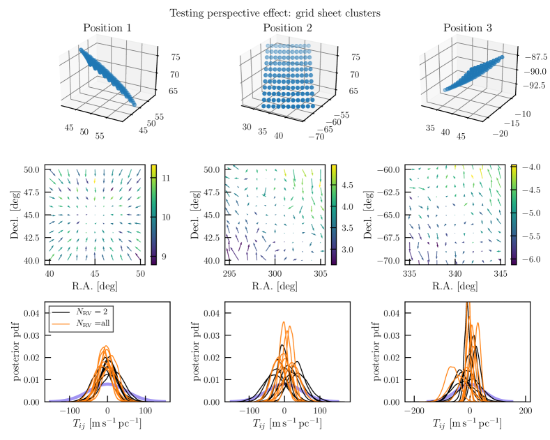
Figure 13: Fitting mock grid sheet clusters at the three positions shown in Figure 12. We show the 3D positions of stars in the top row, the residual proper motion pattern in the middle row (similar as in Figure 12 but with observational noise and internal velocity dispersion of 0.1 $\rm km~{}s^{-1}$) and the inferred velocity gradient matrix components $T_{ij}=dv_{x,y,z}/d{x,y,z}$. In each test case, we assume two scenarios of RV availability: when only two randomly chosen stars have RVs and when all stars have RVs. The posterior distribution of $T_{ij}$ for these two cases are shown in black and orange lines respectively in the bottom panels. The proper motion vectors in the middle row are color-coded by radial velocity indicated in accompanying right color bars. The thick purple line in the bottom panels is the prior distribution of $T_{ij}$. The shrinkage from prior to posterior pdf quantifies how informative the data is. Note that while the prior of $T_{ij}$ may seem narrow for these test cases designed to demonstrate how perspective effect is taken into account, they are quite broad for the real Hyades data.

In order to demonstrate the forward-modelling method fully takes perspective effect into account, we provide two test cases. First, we fit hypothetical grid sheet clusters sampled at the exact grids of $(\alpha\,\delta)$ at each position in Figure 12. Second, we fit hypothetical spherical clusters centred at each position. We use a simplified version of our full model, excluding the mixture component (which accounts for non-member contamination) and assuming isotropic velocity dispersion to fit the mock data. We add 5% Gaussian noise for proper motions and radial velocities, assume parallax errors small enough to resolve the depth of the clusters, and give the clusters a small velocity dispersion of 0.1 $\rm km~{}s^{-1}$. The results are presented in Figure 13 and 14. In each figure, we show the 3D positions of 100 stars in the mock clusters in the top row, the observed (sampled with uncertainty) residual proper motion pattern in the middle row and the inferred posterior pdf of velocity gradient matrix $T_{ij}$ in the bottom row. For each test case, we assumed two possible scenarios of RV availability: when RV is available for only 2 stars (black posterior pdf lines) and when RV is available for all stars (orange posterior pdf lines). In all cases, we correctly infer $T_{ij}=0$ as we should despite the strong apparent proper motion gradients (apparent contraction/rotation/shear). Notice also that while the posterior pdfs of $\mathbf{T}$ are narrower when RVs are available for all stars (as they should be with more information), they are still constrained when RVs are available for only 2 stars. If a few RV measurements across the cluster can ‘anchor’ the radial velocity dimension, then subtle changes in proper motions due to the cluster’s rotation or shear can be correctly inferred as they will introduce systematic residual change on top of the perspective effect.

We conclude this appendix with a final remark that when the parallax errors are too large such that the depth of the cluster is unresolved, the inferred velocity gradient can be non-zero even when its real value is zero. In this case, the cluster will appear to be radially elongated due to noise in the parallax measurement, similar to the “finger of God” effect for galaxy clusters. Because parallaxes give distance information and distances affect proper motions, this will inject correlations between position and velocity, which leads to a non-zero inferred $\mathbf{T}$ even when the real $\mathbf{T}=0$. This is a systematic effect, which puts a lower limit on the smallest $\mathbf{T}$ value that can be inferred from the data. This is unrelated to taking the covariance between parallaxes and proper motions into account, which we do in our method described in Section 2.1, and likely requires a density model for the cluster along with its kinematics.

References

- Anguiano et al. (2018) Anguiano B., Majewski S. R., Freeman K. C., Mitschang A. W., Smith M. C., 2018, MNRAS, 474, 854
- Arenou et al. (2018) Arenou F., et al., 2018, A&A, 616, A17
- Astropy Collaboration et al. (2013) Astropy Collaboration et al., 2013, A&A, 558, A33
- Astropy Collaboration et al. (2018) Astropy Collaboration et al., 2018, AJ, 156, 123
- Baumgardt (2001) Baumgardt H., 2001, MNRAS, 325, 1323
- Belokurov et al. (2020) Belokurov V., et al., 2020, arXiv e-prints, p. arXiv:2003.05467
- Binney & Tremaine (2008) Binney J., Tremaine S., 2008, Galactic Dynamics: Second Edition
- Blaauw (1964) Blaauw A., 1964, in Kerr F. J., ed., IAU Symposium Vol. 20, The Galaxy and the Magellanic Clouds. p. 50
- Bovy (2017) Bovy J., 2017, MNRAS, 468, L63
- Brandt (2018) Brandt T. D., 2018, ApJS, 239, 31
- Bravi et al. (2018) Bravi L., et al., 2018, A&A, 615, A37
- Cantat-Gaudin et al. (2019) Cantat-Gaudin T., et al., 2019, A&A, 626, A17
- Carpenter et al. (2017) Carpenter B., et al., 2017, Journal of Statistical Software, 76, 1
- Choi et al. (2016) Choi J., Dotter A., Conroy C., Cantiello M., Paxton B., Johnson B. D., 2016, ApJ, 823, 102
- Dravins et al. (1999) Dravins D., Lindegren L., Madsen S., 1999, A&A, 348, 1040
- Ernst et al. (2007) Ernst A., Glaschke P., Fiestas J., Just A., Spurzem R., 2007, MNRAS, 377, 465
- Ernst et al. (2011) Ernst A., Just A., Berczik P., Olczak C., 2011, A&A, 536, A64
- Evans & Collett (1993) Evans N. W., Collett J. L., 1993, MNRAS, 264, 353
- Fellhauer et al. (2007) Fellhauer M., et al., 2007, MNRAS, 375, 1171
- Gaia Collaboration et al. (2016) Gaia Collaboration et al., 2016, A&A, 595, A1
- Gaia Collaboration et al. (2018a) Gaia Collaboration et al., 2018a, A&A, 616, A1
- Gaia Collaboration et al. (2018b) Gaia Collaboration et al., 2018b, A&A, 616, A10
- Gao (2019) Gao X.-h., 2019, PASP, 131, 044101
- Gelman & Rubin (1992) Gelman A., Rubin D. B., 1992, Statistical Science, 7, 457
- Gnedin et al. (1999) Gnedin O. Y., Lee H. M., Ostriker J. P., 1999, ApJ, 522, 935
- Gossage et al. (2018) Gossage S., Conroy C., Dotter A., Choi J., Rosenfield P., Cargile P., Dolphin A., 2018, ApJ, 863, 67
- Gunn et al. (1988) Gunn J. E., Griffin R. F., Griffin R. E. M., Zimmerman B. A., 1988, AJ, 96, 198
- Hénon (1961) Hénon M., 1961, Annales d’Astrophysique, 24, 369
- Heyer & Dame (2015) Heyer M., Dame T. M., 2015, ARA&A, 53, 583
- Hoffman & Gelman (2011) Hoffman M. D., Gelman A., 2011, arXiv e-prints, p. arXiv:1111.4246
- Hogg (2018) Hogg D. W., 2018, arXiv e-prints, p. arXiv:1804.07766
- Hogg et al. (2010) Hogg D. W., Bovy J., Lang D., 2010, arXiv e-prints, p. arXiv:1008.4686
- Hunter (2007) Hunter J. D., 2007, Computing in Science and Engineering, 9, 90
- Jeffreson et al. (2017) Jeffreson S. M. R., et al., 2017, MNRAS, 469, 4740
- Just et al. (2009) Just A., Berczik P., Petrov M. I., Ernst A., 2009, MNRAS, 392, 969
- Katz et al. (2019) Katz D., et al., 2019, A&A, 622, A205
- Kim et al. (2019) Kim D., Lu J. R., Konopacky Q., Chu L., Toller E., Anderson J., Theissen C. A., Morris M. R., 2019, AJ, 157, 109
- Kos et al. (2019) Kos J., et al., 2019, A&A, 631, A166
- Kounkel et al. (2018) Kounkel M., et al., 2018, AJ, 156, 84
- Krumholz et al. (2019) Krumholz M. R., McKee C. F., Bland -Hawthorn J., 2019, ARA&A, 57, 227
- Kuhn et al. (2019) Kuhn M. A., Hillenbrand L. A., Sills A., Feigelson E. D., Getman K. V., 2019, ApJ, 870, 32
- Kuijken & Tremaine (1994) Kuijken K., Tremaine S., 1994, ApJ, 421, 178
- Küpper et al. (2008) Küpper A. H. W., MacLeod A., Heggie D. C., 2008, MNRAS, 387, 1248
- Küpper et al. (2010) Küpper A. H. W., Kroupa P., Baumgardt H., Heggie D. C., 2010, MNRAS, 407, 2241
- Lada & Lada (2003) Lada C. J., Lada E. A., 2003, ARA&A, 41, 57
- Leão et al. (2019) Leão I. C., Pasquini L., Ludwig H. G., de Medeiros J. R., 2019, MNRAS, 483, 5026
- Lewandowski et al. (2009) Lewandowski D., Kurowicka D., Joe H., 2009, Journal of Multivariate Analysis, 100, 1989
- Lindegren et al. (2000) Lindegren L., Madsen S., Dravins D., 2000, A&A, 356, 1119
- Lindegren et al. (2018) Lindegren L., et al., 2018, A&A, 616, A2
- McKinney (2010) McKinney W., 2010, in van der Walt S., Millman J., eds, Proceedings of the 9th Python in Science Conference. pp 51 – 56
- Meingast & Alves (2019) Meingast S., Alves J., 2019, A&A, 621, L3
- Milne (1935) Milne E. A., 1935, MNRAS, 95, 560
- Murray (1983) Murray C. A., 1983, Vectorial astrometry. Adam Hilger
- Ogrodnikoff (1932) Ogrodnikoff K., 1932, Z. Astrophys., 4, 190
- Oort (1928) Oort J. H., 1928, Bull. Astron. Inst. Netherlands, 4, 269
- Oort (1979) Oort J. H., 1979, A&A, 78, 312
- Perryman et al. (1998) Perryman M. A. C., et al., 1998, A&A, 331, 81
- Plummer (1911) Plummer H. C., 1911, MNRAS, 71, 460
- Reino et al. (2018) Reino S., de Bruijne J., Zari E., d’Antona F., Ventura P., 2018, MNRAS, 477, 3197
- Röser & Schilbach (2019) Röser S., Schilbach E., 2019, A&A, 627, A4
- Röser et al. (2011) Röser S., Schilbach E., Piskunov A. E., Kharchenko N. V., Scholz R. D., 2011, A&A, 531, A92
- Röser et al. (2019) Röser S., Schilbach E., Goldman B., 2019, A&A, 621, L2
- Smith et al. (2009) Smith M. C., Evans N. W., An J. H., 2009, ApJ, 698, 1110
- Smith et al. (2012) Smith M. C., Whiteoak S. H., Evans N. W., 2012, ApJ, 746, 181
- Spitzer & Chevalier (1973) Spitzer Lyman J., Chevalier R. A., 1973, ApJ, 183, 565
- Spitzer & Hart (1971) Spitzer Lyman J., Hart M. H., 1971, ApJ, 164, 399
- Tang et al. (2018) Tang S.-Y., Chen W. P., Chiang P. S., Jose J., Herczeg G. J., Goldman B., 2018, ApJ, 862, 106
- Tang et al. (2019) Tang S.-Y., et al., 2019, ApJ, 877, 12
- Urquhart et al. (2018) Urquhart J. S., et al., 2018, MNRAS, 473, 1059
- Van Der Walt et al. (2011) Van Der Walt S., Colbert S. C., Varoquaux G., 2011, Computing in Science & Engineering, 13, 22
- Vehtari et al. (2019) Vehtari A., Gelman A., Simpson D., Carpenter B., Bürkner P.-C., 2019, arXiv e-prints, p. arXiv:1903.08008
- Virtanen et al. (2019) Virtanen P., et al., 2019, arXiv e-prints, p. arXiv:1907.10121
- Wright & Mamajek (2018) Wright N. J., Mamajek E. E., 2018, MNRAS, 476, 381
- Wright et al. (2019) Wright N. J., et al., 2019, MNRAS, 486, 2477
- Zari et al. (2019) Zari E., Brown A. G. A., de Zeeuw P. T., 2019, A&A, 628, A123
- de Bruijne et al. (2001) de Bruijne J. H. J., Hoogerwerf R., de Zeeuw P. T., 2001, A&A, 367, 111
- van Leeuwen (2009) van Leeuwen F., 2009, A&A, 497, 209