Numerical evidence for many-body localization in two and three dimensions
Abstract
Disorder and interactions can lead to the breakdown of statistical mechanics in certain quantum systems, a phenomenon known as many-body localization (MBL). Much of the phenomenology of MBL emerges from the existence of -bits, a set of conserved quantities that are quasilocal and binary (i.e., possess only eigenvalues). While MBL and -bits are known to exist in one-dimensional systems, their existence in dimensions greater than one is a key open question. To tackle this question, we develop an algorithm that can find approximate binary -bits in arbitrary dimensions by adaptively generating a basis of operators in which to represent the -bit. We use the algorithm to study four models: the one-, two-, and three-dimensional disordered Heisenberg models and the two-dimensional disordered hard-core Bose-Hubbard model. For all four of the models studied, our algorithm finds high-quality -bits at large disorder strength and rapid qualitative changes in the distributions of -bits in particular ranges of disorder strengths, suggesting the existence of MBL transitions. These transitions in the one-dimensional Heisenberg model and two-dimensional Bose-Hubbard model coincide well with past estimates of the critical disorder strengths in these models which further validates the evidence of MBL phenomenology in the other two and three-dimensional models we examine. In addition to finding MBL behavior in higher dimensions, our algorithm can be used to probe MBL in various geometries and dimensionality.
Introduction.— It is natural to expect quantum systems to obey statistical mechanics. However, there is increasing evidence that there exist disordered strongly interacting quantum systems that do not obey the laws of statistical mechanics and never reach thermal equilibrium – a phenomenon known as many-body localization (MBL) [1, 2, 3, 4, 5, 6, 7]. A key feature of MBL systems is they exhibit robust emergent integrability, i.e., they possess many quasilocal 111In the MBL literature, a “quasilocal” operator refers to an operator that has compact support over a finite region and exponentially decaying tails beyond that region. In other contexts, such as when discussing Anderson localization, such operators would be called local or localized instead. conserved quantities (known as -bits) [9, 10, 11]. The existence of these robust conserved quantities is strongly related to other well-known properties of MBL, such as area-law entanglement of excited states and logarithmic growth of entanglement entropy under time-evolution [5, 6, 7]. Numerical methods have been key to studying MBL [12, 13, 12, 14, 15, 16, 17, 18, 19, 20, 21], but have mostly been limited to small finite-size systems and one spatial dimension.
A key open question that remains is the role of dimensionality in MBL [7]. In one-dimension, there is significant numerical and analytic evidence for MBL phenomena (although even this is still controversial [22]). In higher dimensions, the situation is less clear. Cold-atom experiments show some signatures of slow thermalization in two and three dimensions [23, 24, 25]. Some have argued that MBL phases are unstable to rare ergodic regions that trigger thermalizing avalanches [26, 27]. Others have suggested that an MBL phase might survive but only in nonstandard thermodynamic limits [28, 29, 30]. In this work we take a pragmatic approach and numerically search for -bits in higher dimensions, which we take as a practical signature of MBL. Being able to predict properties of MBL in higher dimensions is also key to making the connection to two and three dimensional cold-atom experiments. While some numerical approaches exist in two-dimensions [31, 32, 33, 34, 35, 36, 37, 38, 39, 40, 41], simulating MBL in higher dimensions is still largely intractable and it is important to develop new numerical techniques, particularly in three-dimensions, where to our knowledge no numerical studies have been done.
In this work, we present a new algorithm for finding approximate -bits (or -bit-like operators [28]) in interacting disordered systems of arbitrary dimensions. In MBL systems, an exact -bit is an operator that (1) is quasilocal, (2) commutes with the Hamiltonian, and (3) has a binary spectrum, i.e., a spectrum of half and half eigenvalues. Our algorithm constructs an approximate -bit by finding an operator that satisfies these three properties as closely as possible. Property (1) is approximated by representing the approximate -bit as a linear combination of finitely many local Pauli strings, while properties (2) and (3) are approximated by minimizing an objective function using gradient descent. Some previously developed numerical methods for finding -bits in MBL systems have attempted to enforce these properties exactly [42, 43, 44, 45, 46, 47]. Other methods have attempted to numerically construct operators that approximately satisfy properties (1) and (2) and either exactly enforce the binary property (3) [33, 48] or do not enforce that property at all [49, 50, 51, 32, 52, 53, 54]. Many of these methods have required numerically expensive calculations, e.g., exact diagonalization or large bond-dimension tensor networks, and, except for the methods of Refs. 32, 33, 35, have been limited to the study of one-dimensional chains. Our algorithm can efficiently produce operators that are reasonable approximations of binary, quasilocal -bits in arbitrary dimensions.
Using our algorithm, we study four model Hamiltonians: the disordered Heisenberg model in one, two, and three-dimensions, and the disordered hard-core Bose-Hubbard model in two-dimensions (also examined in Refs. 35, 36). In all models studied, we find high quality -bits at high disorder strengths suggesting MBL behavior and see statistical signatures of a potential transition from localized to delocalized integrals of motions. Our results provide new evidence for the existence of MBL phenomenology in two and three-dimensions.
Background.— In this work, we investigate two different types of Hamiltonians. First, we consider the disordered spin- Heisenberg model
| (1) |
where the first summation is over nearest neighbor sites of a 1D, 2D, or 3D lattice, are random numbers drawn from a uniform distribution, and is the disorder strength. The 1D model has been extensively investigated numerically, mostly using exact diagonalization [55, 56, 12, 14, 17] and tensor networks [57, 58, 59, 60, 18, 20, 61, 62]. However, the model in higher dimensions has, up to this point, been largely unexplored [32, 39].
Second, we consider the disordered Bose-Hubbard model
| (2) |
where the first summation is over nearest neighbor sites of a two-dimensional square lattice, and are bosonic creation and annihilation operators, , and are random on-site potentials drawn from a Gaussian distribution with full-width half-maximum . This model approximately describes the interactions between bosonic 87Rb atoms in a two-dimensional disordered optical lattice experiment [23], where a potential MBL-ergodic transition was observed at with . Refs. 35 numerically studied this model in the hard-core limit using tensor networks, where they found a transition at ; we too work in this limit.
Generically, a Hamiltonian such as Eq. (1) or (2) can be represented as
| (3) |
where are coupling constants and where is a unitary that diagonalizes the Hamiltonian. The operators are integrals of motion () that mutually commute () and have a binary spectrum ( and ). Note that these operators are not unique since there exist many unitaries that diagonalize . In MBL systems, the operators can be made quasilocal, so that the support of the operators decays rapidly away from a single site on which they are localized, and are known as -bits. A operator can be written as
| (4) |
where is a real coefficient, is a Pauli string (a product of Pauli matrices, such as ), and is a basis of Pauli strings of size . The quasilocality of -bits make it possible to accurately represent them using a small, finite basis of local Pauli strings.
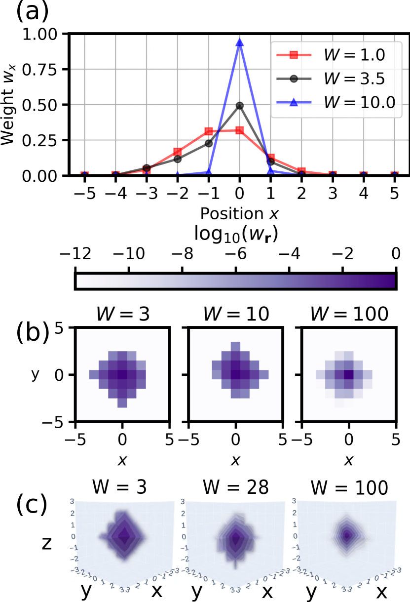
To quantify quasilocality, we can define the weight of a operator [54, 43] as
| (5) |
where is the spatial coordinate of a site in the lattice and is the set of (labels of) Pauli strings in the basis with (non-identity) support on lattice coordinate . The weight decays rapidly in MBL phases, as shown in Fig. 1.
Method.— Our algorithm constructs quasilocal operators that approximately commute with the Hamiltonian and are approximately binary. In particular, the algorithm optimizes the parameters in Eq. (4) to minimize the objective function
| (6) |
where , is the Frobenius norm, and is the identity operator. As described in the supplement 222See Supplemental Material for additional details on the methods used and for additional data obtained in this work. The supplement includes Refs. 77, 78, 79., this minimization is done using gradient descent and Newton’s method. Note that if the second term of Eq. (6) is zero, then the eigenvalues of have exactly equal sectors of eigenvalues because is traceless. Also note that while we do not constrain to be normalized (), it stays approximately normalized during the optimization because of the second term of Eq. (6). We set .
Rather than perform a single minimization of Eq. (6) in a fixed basis , we iteratively and adaptively build the basis during the minimization (similar in spirit to selected configuration interaction, an adaptive basis technique in quantum chemistry [64, 65, 66, 67]). The steps of the algorithm are:
-
1.
Initialize .
-
2.
Expand by adding new Pauli strings.
-
3.
Minimize Eq. (6) in basis .
-
4.
Repeat steps 2–3 while .
In step 1, we initialize the basis with a single Pauli matrix at site . In step 2, we expand the basis by including new Pauli strings that are important for minimizing the objective in Eq. (6). In particular, our heuristic expansion procedure is two-step: (a) first, we compute and add new Pauli strings to with the largest amplitudes 333In order to save memory and time in our calculations, we modified step (a) so that only the largest 2000 terms of were kept before computing .; (b) then, we compute and add new Pauli strings to with the largest amplitudes . The logic behind step (a) is that, to cancel the remainder of , we need to add Pauli strings that, when commuted through the Hamiltonian, coincide with the remainder. These are the terms in . The logic is similar for step (b). In our calculations, we set and perform basis expansions, so that we expand by up to Pauli strings per iteration to a maximum basis size of . In step 3, we perform gradient descent with the parameters in Eq. (4) initialized to the optimized values obtained in the previous basis size, but rescaled so they are normalized to one.
We execute our algorithm on 1D, 2D, and 3D periodic lattices of size , and , respectively. It is important to note that, because of the basis sizes considered, the optimized never reach the lattice boundaries, indicating that our calculations do not exhibit any finite system-size effects or boundary effects, but do exhibit finite basis-size effects.
Results and discussion.— Using our algorithm, we obtain operators for 1600 random realizations of the disordered Heisenberg models of Eq. (1) and for 800 realizations of the disordered hard-core Bose-Hubbard model of Eq. (2) 444We use the same set of (scaled) disorder patterns for all for a fixed model but different disorder patterns for different models.. In this section, we present some statistical properties of the (normalized) operators that our algorithm finds after the final iteration of basis expansions (see supplement for earlier iterations).
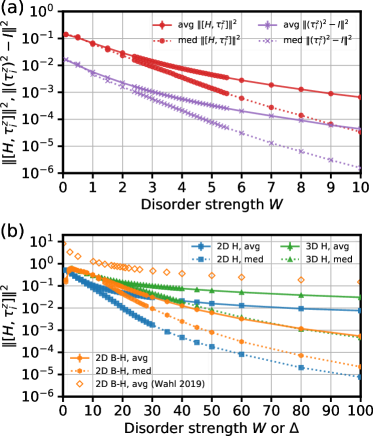
At high disorder, we find operators that are largely binary and nearly commute with the Hamiltonian for all four models studied (see Fig. 2). This is anticipated in an MBL phase where quasilocal operators should be well represented by a small local basis of operators. However, the algorithm’s ability to find good -bits becomes 1–2 orders of magnitude worse with respect to both the commutator norm and binarity with decreasing disorder strength. We also compare the rate of convergence as a function of basis size (see Figs. S23-24 in supplement); while the errors decrease with basis size, they fall off slowly. Improving the rate of convergence is an interesting area for future improvement of the algorithm.
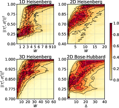
An important statistical quantity that we consider is the overlap 555Note that when we compute this quantity we use the on the site with the largest weight (see Eq. (5)) rather than the used to initialize the basis . In general, the operators discovered with our method can “drift” away from their initial site, though this tends to only become significant at low disorder strength (see supplement). (see Fig. 3 for their distributions). At high disorder, most operators are localized so that , with the distribution exhibiting a quickly decaying tail away from this value. At low disorder, there are almost no operators with ; instead most operators have an overlap with a non-zero value significantly below one. For all the models studied, we find a rapid change in the probability distribution of these operator overlaps over a narrow region of disorder; within this region we see hints of bimodality [16, 17, 13] of the probability distribution. We would anticipate that this rapid change signals a “transition.”
We find in 1D that the location of this transition region is in good agreement with the accepted location of the MBL-ergodic transition in the range [56, 59, 12, 14, 17, 62, 50, 51, 53, 54, 44, 43]. Moreover, the transition region of in the 2D hard-core Bose-Hubbard model is consistent with the critical disorder strength of estimated by Ref. 35. The rapid changes in the probability distributions of in the 2D and 3D Heisenberg models and their high overlap at large disorder then suggests that similar MBL transitions exist in these models as well. These transitions happen around and , respectively. See supplement for details on the estimation of the approximate location of the transition regions.
We note that in 1D, the two peaks of in the transition region are more separated than in higher dimensions. We believe this is due to limitations of the basis size; in 1D, as the basis size grows the separation between the peaks also grows (see supplement) and we expect the same to hold for other models.
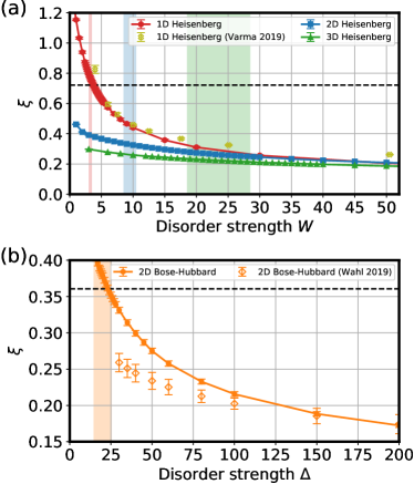
Another quantity we use to characterize is the correlation length, shown in Fig. 4. We obtain correlation lengths by fitting the function to the weight of Eq. (5) for the centered at site using a non-linear least-squares fit 666Note that the summation in the denominator of is only over the positions where and .. We should note that while this fitting procedure gave sensible results for all models, other reasonable ways of fitting these approximate -bits were less robust. For a wide range of disorder strengths, our 1D Heisenberg model correlation lengths agree with those obtained by Ref. 46 (see supplement for additional correlation length comparisons). For large disorder strengths, our 2D Bose-Hubbard correlation lengths agree with those obtained by Ref. 35 using shallow 2D tensor networks, but take on larger values at low disorder strength. As shown in Fig. 2(b), our -bits have significantly lower commutator norms, so might be able to more accurately capture the operators near the transition. As expected theoretically, none of the correlation lengths diverge at the “transition.” Interestingly, we empirically find that , where is the spatial dimension, near the transition region. While the value agrees with some theoretical predictions [46], we are not aware of expected values of correlation lengths at the transition region in higher and these values in larger dimensions might be coincidental.
Finally, we note that for the 2D Bose-Hubbard model we see a sharp change in the histogram of at (see Fig. 3) somewhat close to the value obtained experimentally by Ref. 23. Near this disorder strength the binarity of our -bits increases sharply and so this behavior could simply be attributed to a breakdown of our algorithm (see supplement); nonetheless, we cannot rule out that the algorithm breaking down near this low is somehow related to the results seen in the experimental systems.
Outlook.— We present an algorithm for constructing high-quality approximations of quasilocal binary integrals of motion and use it to study MBL in four different models. This algorithm works by adaptively building a basis of operators in which to construct the quasilocal integrals of motion (-bits). Using this algorithm, we find the first theoretical evidence for MBL in three dimensions.
Our algorithm is well suited for studying -bits in more general settings than has previously been possible. For example, it can be used to construct approximate -bits for models on complicated lattice geometries, for fermionic models (in which Majorana strings can be used instead of Pauli strings; see Ref. 74), or for models with potential MBL-MBL transitions [75]. Moreover, using the strategy of Ref. 32, the -bits constructed with this algorithm could be used to push highly excited states into the ground state. Our algorithm can also be applied beyond MBL to construct localized zero modes in interacting topological systems [76, 74] or (with slight adjustment) to construct unitary operators that commute with given Hamiltonians or symmetries.
Acknowledgements.
Acknowledgments.— We acknowledge useful discussions with Ryan Levy, Greg Hamilton, and David Pekker. We thank Steve Simon, Arijeet Pal, Thorsten Wahl, David Huse, and David Luitz for a careful reading of and comments on the manuscript. We acknowledge support from the Department of Energy grant DOE de-sc0020165. This research is part of the Blue Waters sustained-petascale computing project, which is supported by the National Science Foundation (Awards No. OCI-0725070 and No. ACI-1238993) and the state of Illinois. Blue Waters is a joint effort of the University of Illinois at Urbana-Champaign and its National Center for Supercomputing Applications.References
- Anderson [1958] P. W. Anderson, Absence of Diffusion in Certain Random Lattices, Phys. Rev. 109, 1492 (1958).
- Fleishman and Anderson [1980] L. Fleishman and P. W. Anderson, Interactions and the Anderson transition, Physical Review B 21, 2366 (1980).
- Gornyi et al. [2005] I. V. Gornyi, A. D. Mirlin, and D. G. Polyakov, Interacting electrons in disordered wires: Anderson localization and low-T transport, Phys. Rev. Lett. 95, 206603 (2005).
- Basko et al. [2006] D. M. Basko, I. L. Aleiner, and B. L. Altshuler, Metal–insulator transition in a weakly interacting many-electron system with localized single-particle states, Ann. Phys. (N. Y.) 321, 1126 (2006).
- Nandkishore and Huse [2015] R. Nandkishore and D. A. Huse, Many-body localization and thermalization in quantum statistical mechanics, Annu. Rev. Condens. Matter Phys. 6, 15 (2015).
- Abanin and Papić [2017] D. A. Abanin and Z. Papić, Recent progress in many-body localization, Ann. Phys. (Berl.) 529, 1700169 (2017).
- Abanin et al. [2019] D. A. Abanin, E. Altman, I. Bloch, and M. Serbyn, Colloquium: Many-body localization, thermalization, and entanglement, Rev. Mod. Phys. 91, 021001 (2019).
- Note [1] In the MBL literature, a “quasilocal” operator refers to an operator that has compact support over a finite region and exponentially decaying tails beyond that region. In other contexts, such as when discussing Anderson localization, such operators would be called local or localized instead.
- Serbyn et al. [2013] M. Serbyn, Z. Papić, and D. A. Abanin, Local conservation laws and the structure of the many-body localized states, Phys. Rev. Lett. 111, 127201(R) (2013).
- Huse et al. [2014] D. A. Huse, R. Nandkishore, and V. Oganesyan, Phenomenology of fully many-body-localized systems, Phys. Rev. B 90, 174202 (2014).
- Imbrie et al. [2017] J. Z. Imbrie, V. Ros, and A. Scardicchio, Local integrals of motion in many-body localized systems, Ann. Phys. (Berl.) 529, 1600278 (2017).
- Luitz et al. [2015] D. J. Luitz, N. Laflorencie, and F. Alet, Many-body localization edge in the random-field heisenberg chain, Phys. Rev. B 91, 081103(R) (2015).
- Villalonga et al. [2018] B. Villalonga, X. Yu, D. J. Luitz, and B. K. Clark, Exploring one-particle orbitals in large many-body localized systems, Phys. Rev. B 97, 104406 (2018).
- Serbyn and Moore [2016] M. Serbyn and J. E. Moore, Spectral statistics across the many-body localization transition, Phys. Rev. B 93, 041424(R) (2016).
- Bauer and Nayak [2013] B. Bauer and C. Nayak, Area laws in a many-body localized state and its implications for topological order, J. Stat. Mech. 2013, P09005 (2013).
- Kjäll et al. [2014] J. A. Kjäll, J. H. Bardarson, and F. Pollmann, Many-body localization in a disordered quantum Ising chain, Phys. Rev. Lett. 113, 107204 (2014).
- Yu et al. [2016] X. Yu, D. J. Luitz, and B. K. Clark, Bimodal entanglement entropy distribution in the many-body localization transition, Phys. Rev. B 94, 184202 (2016).
- Yu et al. [2017] X. Yu, D. Pekker, and B. K. Clark, Finding Matrix Product State Representations of Highly Excited Eigenstates of Many-Body Localized Hamiltonians, Phys. Rev. Lett. 118, 017201 (2017).
- Luitz [2016] D. J. Luitz, Long tail distributions near the many-body localization transition, Phys. Rev. B 93, 134201 (2016).
- Khemani et al. [2016] V. Khemani, F. Pollmann, and S. L. Sondhi, Obtaining Highly Excited Eigenstates of Many-Body Localized Hamiltonians by the Density Matrix Renormalization Group Approach, Phys. Rev. Lett. 116, 247204 (2016).
- Lim and Sheng [2016] S. P. Lim and D. N. Sheng, Many-body localization and transition by density matrix renormalization group and exact diagonalization studies, Phys. Rev. B 94, 045111 (2016).
- Panda et al. [2020] R. K. Panda, A. Scardicchio, M. Schulz, S. R. Taylor, and M. Žnidarič, Can we study the many-body localisation transition?, EPL (Europhysics Letters) 128, 67003 (2020).
- Choi et al. [2016] J.-Y. Choi, S. Hild, J. Zeiher, P. Schauß, A. Rubio-Abadal, T. Yefsah, V. Khemani, D. A. Huse, I. Bloch, and C. Gross, Exploring the many-body localization transition in two dimensions, Science 352, 1547 (2016).
- Bordia et al. [2017] P. Bordia, H. Lüschen, S. Scherg, S. Gopalakrishnan, M. Knap, U. Schneider, and I. Bloch, Probing slow relaxation and many-body localization in two-dimensional quasiperiodic systems, Phys. Rev. X 7, 041047 (2017).
- Kondov et al. [2015] S. S. Kondov, W. R. McGehee, W. Xu, and B. DeMarco, Disorder-induced localization in a strongly correlated atomic hubbard gas, Phys. Rev. Lett. 114, 083002 (2015).
- De Roeck and Huveneers [2017] W. De Roeck and F. Huveneers, Stability and instability towards delocalization in many-body localization systems, Phys. Rev. B 95, 155129 (2017).
- De Roeck and Imbrie [2017] W. De Roeck and J. Z. Imbrie, Many-body localization: stability and instability, Philos. Trans. R. Soc. A 375, 20160422 (2017).
- Chandran et al. [2016] A. Chandran, A. Pal, C. R. Laumann, and A. Scardicchio, Many-body localization beyond eigenstates in all dimensions, Phys. Rev. B 94, 144203 (2016).
- Agarwal et al. [2017] K. Agarwal, E. Altman, E. Demler, S. Gopalakrishnan, D. A. Huse, and M. Knap, Rare-region effects and dynamics near the many-body localization transition, Ann. Phys. (Berl.) 529, 1600326 (2017).
- Gopalakrishnan and Huse [2019] S. Gopalakrishnan and D. A. Huse, Instability of many-body localized systems as a phase transition in a nonstandard thermodynamic limit, Phys. Rev. B 99, 134305 (2019).
- Lev and Reichman [2016] Y. B. Lev and D. R. Reichman, Slow dynamics in a two-dimensional Anderson-Hubbard model, EPL 113, 46001 (2016).
- Inglis and Pollet [2016] S. Inglis and L. Pollet, Accessing many-body localized states through the generalized gibbs ensemble, Phys. Rev. Lett. 117, 120402 (2016).
- Thomson and Schiró [2018] S. J. Thomson and M. Schiró, Time evolution of many-body localized systems with the flow equation approach, Phys. Rev. B 97, 060201(R) (2018).
- Kennes [2018] D. M. Kennes, Many-Body Localization in Two Dimensions from Projected Entangled-Pair States, (2018), arXiv:1811.04126 .
- Wahl et al. [2019] T. Wahl, A. Pal, and S. Simon, Signatures of the many-body localized regime in two dimensions, Nat. Phys 15, 164 (2019).
- Geißler and Pupillo [2019] A. Geißler and G. Pupillo, Many-body localization in the two dimensional Bose-Hubbard model, (2019), arXiv:1909.09247 .
- De Tomasi et al. [2019] G. De Tomasi, F. Pollmann, and M. Heyl, Efficiently solving the dynamics of many-body localized systems at strong disorder, Phys. Rev. B 99, 241114(R) (2019).
- Théveniaut et al. [2019] H. Théveniaut, Z. Lan, and F. Alet, Many-body localization transition in a two-dimensional disordered quantum dimer model, (2019), arXiv:1902.04091 .
- Kshetrimayum et al. [2019] A. Kshetrimayum, M. Goihl, and J. Eisert, Time evolution of many-body localized systems in two spatial dimensions, (2019), arXiv:1910.11359 .
- Pietracaprina and Alet [2020] F. Pietracaprina and F. Alet, Probing many-body localization in a disordered quantum dimer model on the honeycomb lattice, (2020), arXiv:2005.10233 .
- Doggen et al. [2020] E. V. H. Doggen, I. V. Gornyi, A. D. Mirlin, and D. G. Polyakov, Slow many-body delocalization beyond one dimension, (2020), arXiv:2002.07635 .
- Pekker et al. [2017] D. Pekker, B. K. Clark, V. Oganesyan, and G. Refael, Fixed points of wegner-wilson flows and many-body localization, Phys. Rev. Lett. 119, 075701 (2017).
- Kulshreshtha et al. [2018] A. K. Kulshreshtha, A. Pal, T. B. Wahl, and S. H. Simon, Behavior of l-bits near the many-body localization transition, Phys. Rev. B 98, 184201 (2018).
- Goihl et al. [2018] M. Goihl, M. Gluza, C. Krumnow, and J. Eisert, Construction of exact constants of motion and effective models for many-body localized systems, Phys. Rev. B 97, 134202 (2018).
- Yu et al. [2019] X. Yu, D. Pekker, and B. K. Clark, Bulk Geometry of the Many Body Localized Phase from Wilson-Wegner Flow, (2019), arXiv:1909.11097 .
- Varma et al. [2019] V. K. Varma, A. Raj, S. Gopalakrishnan, V. Oganesyan, and D. Pekker, Length scales in the many-body localized phase and their spectral signatures, Phys. Rev. B 100, 115136 (2019).
- Peng et al. [2019] P. Peng, Z. Li, H. Yan, K. X. Wei, and P. Cappellaro, Comparing many-body localization lengths via nonperturbative construction of local integrals of motion, Phys. Rev. B 100, 214203 (2019).
- Kelly et al. [2020] S. P. Kelly, R. Nandkishore, and J. Marino, Exploring many-body localization in quantum systems coupled to an environment via wegner-wilson flows, Nucl. Phys. B 951, 114886 (2020).
- Kim et al. [2015] H. Kim, M. C. Bañuls, J. I. Cirac, M. B. Hastings, and D. A. Huse, Slowest local operators in quantum spin chains, Phys. Rev. E 92, 012128 (2015).
- Chandran et al. [2015] A. Chandran, I. H. Kim, G. Vidal, and D. A. Abanin, Constructing local integrals of motion in the many-body localized phase, Phys. Rev. B 91, 085425 (2015).
- O’Brien et al. [2016] T. E. O’Brien, D. A. Abanin, G. Vidal, and Z. Papić, Explicit construction of local conserved operators in disordered many-body systems, Phys. Rev. B 94, 144208 (2016).
- Lin and Motrunich [2017] C.-J. Lin and O. I. Motrunich, Explicit construction of quasiconserved local operator of translationally invariant nonintegrable quantum spin chain in prethermalization, Phys. Rev. B 96, 214301 (2017).
- Mierzejewski et al. [2018] M. Mierzejewski, M. Kozarzewski, and P. Prelovšek, Counting local integrals of motion in disordered spinless-fermion and hubbard chains, Phys. Rev. B 97, 064204 (2018).
- Pancotti et al. [2018] N. Pancotti, M. Knap, D. A. Huse, J. I. Cirac, and M. C. Bañuls, Almost conserved operators in nearly many-body localized systems, Phys. Rev. B 97, 094206 (2018).
- Oganesyan and Huse [2007] V. Oganesyan and D. A. Huse, Localization of interacting fermions at high temperature, Phys. Rev. B 75, 155111 (2007).
- Pal and Huse [2010] A. Pal and D. A. Huse, Many-body localization phase transition, Phys. Rev. B 82, 174411 (2010).
- Žnidarič et al. [2008] M. Žnidarič, T. Prosen, and P. Prelovšek, Many-body localization in the Heisenberg magnet in a random field, Phys. Rev. B 77, 064426 (2008).
- Bardarson et al. [2012] J. H. Bardarson, F. Pollmann, and J. E. Moore, Unbounded growth of entanglement in models of many-body localization, Phys. Rev. Lett. 109, 017202 (2012).
- Luca and Scardicchio [2013] A. D. Luca and A. Scardicchio, Ergodicity breaking in a model showing many-body localization, EPL 101, 37003 (2013).
- Pollmann et al. [2016] F. Pollmann, V. Khemani, J. I. Cirac, and S. L. Sondhi, Efficient variational diagonalization of fully many-body localized Hamiltonians, Phys. Rev. B 94, 041116(R) (2016).
- Pekker and Clark [2017] D. Pekker and B. K. Clark, Encoding the structure of many-body localization with matrix product operators, Phys. Rev. B 95, 035116 (2017).
- Wahl et al. [2017] T. B. Wahl, A. Pal, and S. H. Simon, Efficient representation of fully many-body localized systems using tensor networks, Phys. Rev. X 7, 021018 (2017).
- Note [2] See Supplemental Material for additional details on the methods used and for additional data obtained in this work. The supplement includes Refs. \rev@citealpscipy2020,Canovi2011,Rademaker2017.
- Bender and Davidson [1969] C. F. Bender and E. R. Davidson, Studies in Configuration Interaction: The First-Row Diatomic Hydrides, Phys. Rev. 183, 23 (1969).
- Whitten and Hackmeyer [1969] J. L. Whitten and M. Hackmeyer, Configuration Interaction Studies of Ground and Excited States of Polyatomic Molecules. I. The CI Formulation and Studies of Formaldehyde, J. Chem. Phys. 51, 5584 (1969).
- Holmes et al. [2016] A. A. Holmes, N. A. Tubman, and C. J. Umrigar, Heat-Bath Configuration Interaction: An Efficient Selected Configuration Interaction Algorithm Inspired by Heat-Bath Sampling, J. Chem. Theory Comput. 12, 3674 (2016).
- Tubman et al. [2016] N. M. Tubman, J. Lee, T. Y. Takeshita, M. Head-Gordon, and K. B. Whaley, A deterministic alternative to the full configuration interaction quantum monte carlo method, J. Chem. Phys. 145, 044112 (2016).
- Note [3] In order to save memory and time in our calculations, we modified step (a) so that only the largest 2000 terms of were kept before computing .
- Chertkov [2020] E. Chertkov, BIOMS: Binary Integrals of Motion, https://github.com/ClarkResearchGroup/bioms (2020).
- Chertkov [2019] E. Chertkov, Qosy: Quantum Operators from Symmetry, https://github.com/ClarkResearchGroup/qosy (2019).
- Note [4] We use the same set of (scaled) disorder patterns for all for a fixed model but different disorder patterns for different models.
- Note [5] Note that when we compute this quantity we use the on the site with the largest weight (see Eq. (5)) rather than the used to initialize the basis . In general, the operators discovered with our method can “drift” away from their initial site, though this tends to only become significant at low disorder strength (see supplement).
- Note [6] Note that the summation in the denominator of is only over the positions where and .
- Chertkov et al. [2020] E. Chertkov, B. Villalonga, and B. K. Clark, Engineering topological models with a general-purpose symmetry-to-Hamiltonian approach, Phys. Rev. Research 2, 023348 (2020).
- Pekker et al. [2014] D. Pekker, G. Refael, E. Altman, E. Demler, and V. Oganesyan, Hilbert-glass transition: New universality of temperature-tuned many-body dynamical quantum criticality, Phys. Rev. X 4, 011052 (2014).
- Katsura et al. [2015] H. Katsura, D. Schuricht, and M. Takahashi, Exact Ground States and Topological Order in Interacting Kitaev/Majorana Chains, Phys. Rev. B 92, 115137 (2015).
- Virtanen et al. [2020] P. Virtanen et al., SciPy 1.0: Fundamental Algorithms for Scientific Computing in Python, Nature Methods 17, 261 (2020).
- Canovi et al. [2011] E. Canovi, D. Rossini, R. Fazio, G. E. Santoro, and A. Silva, Quantum quenches, thermalization, and many-body localization, Phys. Rev. B 83, 094431 (2011).
- Rademaker et al. [2017] L. Rademaker, M. Ortuño, and A. M. Somoza, Many-body localization from the perspective of Integrals of Motion, Ann. Phys. (Berl.) 529, 1600322 (2017).