Fermionic dualities with axial gauge fields

Abstract

The dualities that map hard-to-solve, interacting theories to free, non-interacting ones often trigger a deeper understanding of the systems to which they apply. However, simplifying assumptions such as Lorentz invariance, low dimensionality, or the absence of axial gauge fields, limit their application to a broad class of systems, including topological semimetals. Here we derive several axial field theory dualities in 2+1 and 3+1 dimensions by developing an axial slave-rotor approach capable of accounting for the axial anomaly. Our 2+1-dimensional duality suggests the existence of a dual, critical surface theory for strained three-dimensional non-symmorphic topological insulators. Our 3+1-dimensional duality maps free Dirac fermions to Dirac fermions coupled to emergent U(1) and Kalb-Ramond vector and axial gauge fields. Upon fixing an axial field configuration that breaks Lorentz invariance, this duality maps free to interacting Weyl semimetals, thereby suggesting that the quantization of the non-linear circular photogalvanic effect can be robust to certain interactions. Our work emphasizes how axial and Lorentz-breaking dualities improve our understanding of topological matter.

I Introduction

A defining property of massless relativistic fermions is that their momentum is either aligned or anti-aligned with their spin. This quantum-mechanical degree of freedom is distinguished by axial gauge fields, which dramatically affect observables in a broad set of physical systems: from strained graphene and Weyl semimetals Amorim et al. (2016); Ilan et al. (2020), to the quark-gluon plasma created in heavy ion collisions Kharzeev (2015). For example, in 3+1 dimensions the absence of axial charge conservation due to quantum fluctuations, known as the axial anomaly Bertlmann (1996), significantly enhances the magnetoconductivity of Weyl semimetals Armitage et al. (2018). Within the quark-gluon plasma an axial chemical potential can generate a current parallel to a magnetic field, an otherwise absent phenomenon known as the chiral magnetic effect Fukushima et al. (2008).

Although axial gauge fields are physically ubiquitous, quantum field theory dualities are typically formulated without them. A quantum field theory duality is a map that renders two quantum field theories equivalent Savit (1980). They are especially useful when a strongly interacting theory that is hard to solve is mapped onto a free quantum field theory. An important recent example is the map proposed by Son Son (2015) between a free 2+1-dimensional Dirac cone and 2+1-dimensional quantum electrodynamics (QED₃), see Ref. Senthil et al. (2019) for a review. It is a fermionic generalization of an older 2+1-dimensional boson-vortex duality Peskin (1978); Dasgupta and Halperin (1981), and its discovery suggested that the composite fermions describing the fractional quantum Hall state of a half-filled Landau level can be Dirac particles Mross et al. (2016). Son’s fermionic duality has also been formulated as a duality between two surface theories, which correspond to two dual 3D topological insulator bulk theories Metlitski and Vishwanath (2016); Wang and Senthil (2015). This duality is embedded within a larger duality web Seiberg et al. (2016); Karch and Tong (2016); Benini (2018); Murugan and Nastase (2017), where different bosonic and fermionic theories can be related to each other by duality transformations. There are variations that consider more than one fermionic flavor Karch and Tong (2016); Xu and You (2015); Sodemann et al. (2017); Jensen and Patil (2019); Chen and Zimet (2018); Potter et al. (2017), as well as proposed extensions to 3+1 dimensions Sagi et al. (2018); Palumbo (2020); Bi and Senthil (2019); Wan and Wang (2019); Furusawa and Nishida (2019).

The description of a growing variety of systems in terms of axial gauge fields challenges us to develop dualities that can be used to understand their interacting phases. Moreover, it is known that the parity anomaly Niemi and Semenoff (1983) is central to Son’s 2+1-dimensional duality Burkov (2019), yet a comparable understanding of the axial anomaly in putative 3+1 dimenisional fermionic dualities is still lacking. Our goal is to formulate dualities that help answer these questions.

In this work we derive several axial field theory dualities in 2+1 and 3+1 dimensions, summarized in Figs. 1 and 2. In 2+1 dimensions the helicity operator is well defined Li et al. (2013), unlike chirality . This implies that a (helical) gauge field can distinguish Dirac fermions by their helicity Cortijo et al. (2010). The duality we derive maps two helical Dirac fermions coupled to external vector and helical gauge fields, into two helical Dirac fermions coupled to mixed Chern-Simons terms that couple the emergent vector and helical U(1) fields with the external fields. Our 2+1-dimensional duality suggests the existence of a surface theory dual to the surface Dirac fermion doublet found in strained 3D non-symmorphic topological insulators Wieder et al. (2018).

In 3+1 dimensions the duality we derive maps two Weyl fermions coupled to a vector ($A_{\mu}$) and an axial gauge field ($A_{5,\mu}$) to an interacting theory with two emergent U(1) vector fields ($a_{\mu}$ and $a_{5,\mu}$) and two emergent Kalb-Ramond fields ($B_{\mu\nu}$ and $B_{5,\mu\nu}$). The latter are anti-symmetric tensor gauge fields that originated in string theory Kalb and Ramond (1974); Banks and Seiberg (2011), and that appear in recent descriptions of 3+1-dimensional topological insulator theories Cho and Moore (2011); Chan et al. (2013); Cirio et al. (2014); Maciejko et al. (2014); Putrov et al. (2017). Interestingly, our 3+1-dimensional duality applies to specific configurations of $A_{5,\mu}$ which describe different topological states, such as the 3D quantum Hall effect Ramamurthy and Hughes (2015); Galeski et al. (2020); Thakurathi and Burkov (2020), and Weyl semimetals Wan et al. (2011). For example, the latter is recovered by choosing a constant $A_{5,\mu}$ on one side of the duality Zyuzin and Burkov (2012); Grushin (2012); Zyuzin et al. (2012); Goswami and Tewari (2013), which breaks Lorentz symmetry and sets the Weyl node separation in momentum and energy space. In this case we find a duality between a Weyl semimetal, described by Lorentz-breaking QED with a constant axial four-vector Colladay and Kostelecký (1997, 1998); Grushin (2012), and Lorentz breaking QED with a dynamical gauge field coupled to a Carroll-Field-Jackiw term Carroll et al. (1990). We show that this duality satisfies a requirement imposed by Son’s fermionic duality. The non-interacting side of our Weyl semimetal duality is known to display an exactly quantized circular photogalvanic effect de Juan et al. (2017), a non-linear photocurrent generated by circularly polarized light. Our duality implies that the dual interacting theory must present the same quantized circular photogalvanic effect. This is in contrast to the effect of more conventional Coulomb interactions which correct the quantization constant if present Avdoshkin et al. (2020).

To derive the dualities presented here we have developed an axial slave-rotor transformation that generalizes the slave-rotor technique Florens and Georges (2002, 2004), and incorporates the chiral anomaly in 3+1 dimensions. It is inspired by the work in Ref. Burkov and Balents (2011), where this technique has been used to derive Son’s duality and to emphasize the key role played by the parity anomaly Niemi and Semenoff (1983).

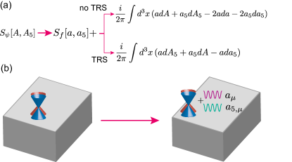
Figure 1: Schematic summary of the 2+1-dimensional axial dualities discussed in this work. (a) A theory of two helical massless fermions $\psi$ is coupled an external vector ($A_{\mu}$) and helical gauge fields ($A_{5,\mu}$). Physically, this can describe the double Dirac surface state of a strained non-symmorphic topological insulator. Depending on the realization of time-reversal symmetry, this theory maps to two different extensions of QED₃ of neutral fermions $f$, with mutual Chern-Simons coupling the two external fields with two emergent vector and helical fields, $a_{\mu}$ and $a_{5,\mu}$. (b) These dualities suggest the existence of dual surface theories for the double Dirac surface state of a strained non-symmorphic topological insulator.

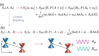
Figure 2: Schematic summary of the 3+1-dimensional axial dualities discussed in this work. (a) A massless Dirac fermion in 3+1-dimensions $\psi$, coupled to an external vector ($A_{\mu}$) and chiral ($A_{5,\mu}$) gauge fields is dual to a neutral Dirac fermion $f$ coupled to vector and axial dynamical gauge fields ($a_{\mu}$ and $a_{5,\mu}$), and a vector and axial Kalb-Ramond fields ($B_{\rho\sigma}$ and $B_{5,\rho\sigma}$) through terms of the form $\epsilon^{\mu\nu\rho\sigma}F_{\mu\nu}B_{\rho\sigma}$, known as BF terms. The last term accounts for the chiral anomaly. (b) When $A_{5,\mu}$ is set to a constant ($-b_{\mu}$), Lorentz symmetry is broken and the non-interacting theory describes a Weyl semimetal with Weyl node separation set by $b_{\mu}$. Its dual is an interacting Weyl semimetal theory with a BF, and mixed Carroll-Field-Jackiw terms. This duality suggests that an interacting Weyl theory can display a quantized photogalvanic effect.

II Axial slave-rotor approach

Our goal is to derive dualities between theories that contain two types of fermions, either with opposite helicity in 2+1 dimensions, or with opposite chirality in 3+1 dimensions. We therefore start by generalizing the slave-rotor approach Florens and Georges (2002, 2004) to incorporate chirality and helicity. The method allows us to describe interactions in terms of two emergent Abelian gauge fields, and can be viewed as the U(1)_V $\times$ U(1)_A descendant of the SU(2) non-Abelian constructions in Refs. Hermele (2007); Xu (2010). In our case, U(1)_V is associated to a vector gauge symmetry while U(1)_A is associated to an axial gauge symmetry.

Our starting point is a system that can be decomposed into two independent sectors, that we call $L$ and $R$, such that the total Hilbert space $\mathcal{H}$ is

$$\mathcal{H}\equiv\mathcal{H}_{L}\oplus\mathcal{H}_{R}.$$ (1)

Here $\mathcal{H}_{\chi}$ is the Hilbert space associated to each sector $\chi=L,R$. These sectors are defined by the number operators at a given site $r$, $n_{\chi}$, which are independently conserved at classical level. To describe the physical fermions $\psi_{\chi}$, we introduce two independent rotor fields $\theta_{\chi}$, conjugate to $n_{r,\chi}$, satisfying the following relations

$$\psi_{r,\chi}=e^{-i\theta_{r,\chi}}f_{r,\chi},\hskip 8.5359pt\psi^{\dagger}_{r,\chi}=f^{\dagger}_{r,\chi}\,e^{i\theta_{r,\chi}},$$ (2)

such that

$$[\theta_{r,\chi},n_{r,\chi}]=i.$$ (3)

The operators $e^{i\theta_{r,\chi}}$ create a charged, spinless boson in the $\chi$ sectors. The operators $f^{\dagger}_{r,\chi}$ create neutral spinons that carry the electron’s spin. In using Eq. (2) we pay the price of enlarging the Hilbert space Florens and Georges (2002, 2004). To recover the physical Hilbert space in each sector it is necessary to impose the constraint

$$f^{\dagger}_{r,\chi}f_{r,\chi}=n_{r,\chi}+1.$$ (4)

These constraints act independently on each $\mathcal{H}_{\chi}$, and will be imposed at the level of the action with a Lagrange multiplier. As in previous works Burkov (2019); Palumbo (2020), we assume here that $\langle e^{i\theta_{r,L}}\rangle\neq 0$ and $\langle e^{i\theta_{r,R}}\rangle\neq 0$, which implies the absence of a Mott insulating phase Pesin and Balents (2010).

III 2+1 Fermion-Fermion duality with an axial gauge field

III.1 Formulation of the duality

In 2+1 dimensions there is no notion of chirality. However, two Dirac fermions can form a reducible $4\times 4$ representation of the Clifford algebra, such that the $2\times 2$ irreducible blocks that compose this representation can be labeled by their helicity (left and right), to which an axial gauge field can couple to. In what follows we use the axial slave-rotor approach presented in the previous section to connect two theories involving massless Dirac fermions of opposite helicities. The first theory is a non-interacting theory of two helical massless Dirac fermions in Euclidean spacetime, defined as

$$S_{h} = \int d^{3}x\,\bar{\psi}\gamma^{\mu}(\partial_{\mu}-iA_{\mu}-iA_{5,\mu}\gamma_{5})\psi$$

$$\equiv \int d^{3}x\,\left[\bar{\psi}_{L}\,\sigma^{\mu}_{L}(\partial_{\mu}-iA_{\mu,L})\psi_{L}\right.$$

$$+ \left.\bar{\psi}_{R}\,\sigma^{\mu}_{R}(\partial_{\mu}-iA_{\mu,R})\psi_{R}\right],$$ (5b)

where $A_{\mu}$ is an external electromagnetic field, $A_{5,\mu}$ is an axial gauge field, $\psi=(\psi_{L},\psi_{R})^{T}$ is a four-component spinor, $\sigma^{\mu}_{L}=(\mathbb{I},\sigma^{i})$, ${\sigma}^{\mu}_{R}=(\mathbb{I},-\sigma^{i})$, and

$$A_{\mu,L}=A_{\mu}+A_{5,\mu},$$ (6a)

$$A_{\mu,R}=A_{\mu}-A_{5,\mu}.$$ (6b)

We find this theory to be dual to neutral Dirac fermions $f$ coupled to an emergent vector and axial gauge field, $a_{\mu}$ and $a_{5,\mu}$, respectively. These emergent gauge fields are coupled with the external $A_{\mu}$ and $A_{5,\mu}$ fields through mixed Chern-Simons terms. If time-reversal symmetry is absent, then the dual theory to Eqs. (5) takes the following form

$$S^{(1)}_{\mathrm{cQED_{3}}} = \int d^{3}x\,\bar{f}\gamma^{\mu}(\partial_{\mu}-ia_{\mu}-i\gamma_{5}a_{5,\mu})f$$

$$+ \dfrac{i}{2\pi}adA+\dfrac{i}{2\pi}a_{5}dA_{5}-\dfrac{i}{4\pi}ada-\dfrac{i}{4\pi}a_{5}da_{5}+\cdots.$$

Here we make use of the short hand differential form notation $$ada=\epsilon^{\mu\nu\rho}a_{\mu}\partial_{\nu}a_{\rho} +\cdots$$. In the ellipses () we include higher-derivative kinematic Maxwell terms, which can be neglected to lowest order, and are not relevant for our discussion. When the axial gauge fields are switched off, the duality between Eqs. (5) and (7) reduce to two copies of Son’s duality Son (2015); Sodemann et al. (2017), one for each helicity. If time-reversal symmetry is preserved then the dual theory of Eqs. (5) is given by

$$S^{(2)}_{\mathrm{cQED_{3}}} = \int d^{3}x\,\bar{f}\gamma^{\mu}(\partial_{\mu}-ia_{\mu}-i\gamma_{5}a_{5,\mu})f$$ (7b)

$$+ \dfrac{i}{2\pi}adA_{5}+\dfrac{i}{2\pi}a_{5}dA-\dfrac{i}{2\pi}ada_{5}+\cdots.$$

These are the main results of this section, and are summarized in Fig. 1.

III.2 Derivation of the duality

We begin by defining a lattice version of the gapless Hamiltonian of Eq. (5), given by two decoupled Hamiltonians

$$H=H_{L}+H_{R},$$ (8)

where the Hamiltonian of each sector is given by

$$H_{\chi} = \sum_{r}\left[\psi^{\dagger}_{r,\chi}\left(\frac{-i\hat{\chi}\sigma^{s}-m_{\chi}\sigma^{z}}{2}\right)e^{-iA_{r,r+\hat{s},\chi}}\psi_{r+\hat{s},\chi}+{\rm h.c.}\right]$$ (9)

$$+ \sum_{r}\psi^{\dagger}_{r,\chi}\left[(m_{0}+2m_{\chi})\sigma^{z}-iA_{0,r,\chi}\right]\psi_{r,\chi}.$$

Here $r=\{x,y\}$ is the site index, $A_{r,r+\hat{s},\chi}$ is introduced through a Peierls substitution on the lattice link $(r,r+\hat{s})$ with $\hat{s}\equiv(\hat{x},\hat{y})$. We have also introduced the scalar $\hat{\chi}$ that takes the value $\hat{\chi}=+1$ and $\hat{\chi}=-1$ for chiralities $\chi=L$ and $\chi=R$, respectively. The parameter $m_{0}$ sets the gap at the $\Gamma$ point, while a combination of $m_{0}$ and $m_{\chi}$ sets the gaps at momenta ${\bf{K}}_{i}=(0,\pi),(\pi,0)$ and $(\pi,\pi)$. When $m_{0}=0$, the low-energy theory around $\Gamma$ takes the form of a gapless Dirac fermion

$$H_{\chi} = \hat{\chi}\int d^{3}k\hskip 2.84526pt\bar{\psi}_{k,\chi}\hskip 2.84526pt\sigma^{i}k_{i}\hskip 2.84526pt\psi_{k,\chi}.$$ (10)

For a finite $m_{0}$, the theory becomes that of a massive Dirac fermion that may be integrated out. The resulting effective field theory takes the form of a Chern-Simons theory Niemi and Semenoff (1983)

$$S_{\mathrm{eff}} = -i\dfrac{\mathrm{sgn}(m_{0})}{8\pi}\int d^{3}x\;\epsilon^{\mu\nu\rho}A_{\mu,\chi}\partial_{\nu}A_{\rho,\chi}$$ (11)

$$\equiv -i\dfrac{\mathrm{sgn}(m_{0})}{8\pi}\int d^{3}x\;A_{\chi}dA_{\chi}.$$

where in the second line we have defined a short-hand notation for the Chern-Simons term.

Accordingly, the low-energy theories around ${\bf{K}}_{i}$ are gapped Dirac fermions with masses set by a combination of $m_{0}$ and $m_{\chi}$. We are interested in the limit of small $m_{0}$, for which the combined effective action including ${\bf{K}}_{i}$ is Niemi and Semenoff (1983)

$$S_{\mathrm{eff,\chi}} = i\dfrac{\mathrm{sgn}(m_{\chi})}{8\pi}\int d^{3}x\;A_{\chi}dA_{\chi}.$$ (12)

The role of time-reversal symmetry is explicit when we set $A_{5,\mu}=0$, and therefore $A_{\mu,L}=A_{\mu,R}=A_{\mu}$. If a Chern-Simons term $AdA$ is present in the total effective action, this implies a finite Hall conductivity and the breaking of time-reversal symmetry. The total effective action is obtained by combining Eq. (11) and Eq. (12) for both $\chi$ sectors:

$$S_{\mathrm{eff}} = \frac{i}{8\pi}\int d^{3}x\,\left(-\mathrm{sgn}(m_{0})+\mathrm{sgn}(m_{L})\right)AdA$$ (13)

$$\pm \left(-\mathrm{sgn}(m_{0})+\mathrm{sgn}(m_{R})\right)AdA.$$

The relative sign between $m_{0}$ and $m_{\chi}$ determines whether a Chern-Simons term $AdA$ is allowed within each sector, and therefore sets their respective Hall conductivities. The $\pm$ represents the freedom to choose the relative sign between the Hall conductivities of the $L$ and $R$ sectors.

Since each $\chi$ sector is described by the Hamiltonian considered in Ref. Burkov (2019), we can use the two independent slave-rotor transformations, introduced in the previous section, to find the dual theory of Eqs. (5). For each $\chi$, the derivation follows the method in Ref. Burkov (2019), but here we will keep track of the signs of the different Chern-Simons terms that are induced via the parity anomaly. Because both sectors remain decoupled, we detail the derivation for the dual action for the $L$ sector only. At the end, we will combine both chiral sectors into a single theory by considering the role of time-reversal symmetry.

Using the slave-rotor transformation Eq. (2) we can write the imaginary-time action ($\tau=it$) that corresponds to $H_{L}$ as

$$S=\int_{0}^{\beta}d\tau\sum_{r,s}\left[f_{r,L}^{\dagger}\partial_{\tau}f_{r,L}-in_{r,L}(\partial_{\tau}\theta_{r,L}+A_{r,0,L})\right.\hskip 11.38092pt$$

$$\left.+(m_{0}+2m_{L})f_{r,L}^{\dagger}\sigma_{z}f_{r,L}+i\lambda_{r,L}(f_{r,L}^{\dagger}f_{r,L}-n_{r,L}-1)\right.$$

$$\left.+f_{r,L}^{\dagger}\left(\frac{-i\sigma^{s}-m_{L}\sigma^{z}}{2}\right)e^{-i(A_{r,r+\hat{s},L}+\Delta_{s}\theta_{r,L})}f_{r+\hat{s},L}\right.$$

$$\left.+{\rm h.c.}\right],\hskip 14.22636pt$$ (14)

where $\Delta_{s}\theta_{r,L}=\theta_{r+\hat{s},L}-\theta_{r,L}$ and $\lambda_{r,L}$ is a Lagrange multiplier field that imposes the constraint Eq. (4). To decouple the $f$ fermions from the rotor and external gauge fields, $\theta_{r,\chi}$ and $A_{r,\chi}$, respectively, we introduce a Hubbard-Stratonovich field $h_{L}\equiv\zeta_{L}e^{ia_{L}}$ defined on the lattice Lee and Lee (2005); Barkeshli and McGreevy (2012). Since the amplitude fluctuations are gapped, we can fix the magnitude $\zeta_{L}$ to its saddle point value and consider only phase fluctuations. In this case, Eq. (III.2) can be rewritten as follows:

$$S = \int_{0}^{\beta}d\tau\sum_{r,s}\left[f_{r,L}^{\dagger}(\partial_{\tau}+ia_{r,0,L})f_{r,L}-in_{r,L}(\partial_{\tau}\theta_{r,L}+A_{r,0,L}+a_{r,0,L})+(m_{0}+2m_{L})f_{r,L}^{\dagger}\sigma_{z}f_{r,L}\right.$$ (15)

$$+ \left.\left[\zeta_{L}f_{r,L}^{\dagger}\left(\frac{-i\sigma^{s}-m_{L}\sigma^{z}}{2}\right)e^{ia_{r,r+\hat{s},L}}f_{r+\hat{s},L}+{\rm h.c.}\right]-\zeta_{L}\cos\left(\Delta_{\hat{s}}\theta_{r,L}+A_{r,r+\hat{s},L}+a_{r,r+\hat{s},L}\right)\right],$$

where we have identified the Lagrange multiplier with the temporal component of the emergent gauge field, $a_{r,0,L}\equiv\lambda_{r,L}$. We now may use the Villain approximation to approximate the last cosine as Villain, J. (1975)

$$e^{\zeta\cos(\alpha)}\approx\sum_{J}e^{-iJ\alpha-(1/2\zeta)J^{2}},$$ (16)

at the expense of introducing a boson current $J^{r,r+\hat{s}}_{L}$. After this step, the full action consists of two terms

$$S=S_{f}+S_{\theta},$$ (17)

where

$$S_{f} = \int_{0}^{\beta}d\tau\sum_{r,s}\left[f_{r,L}^{\dagger}(\partial_{\tau}+ia_{r,0,L})f_{r,L}\right.$$

$$+ \left.(m_{0}+2m_{L})f_{r,L}^{\dagger}\sigma_{z}f_{r,L}\right.$$

$$+ \left.\zeta_{L}f_{r,L}^{\dagger}\left(\frac{-i\sigma^{s}-m_{L}\sigma^{z}}{2}\right)e^{ia_{r,r+\hat{s},L}}f_{r+\hat{s},L}+{\rm h.c.}\right],$$

and

$$S_{\theta} = \int_{0}^{\beta}d\tau\sum_{r,s}\left[iJ^{r,0}_{L}(\partial_{\tau}\theta_{r,L}+A_{r,0,L}+a_{r,0,L})\right.$$ (19)

$$+ iJ^{r,r+\hat{s}}_{L}\left(\Delta_{\hat{s}}\theta_{r,L}+A_{r,r+\hat{s},L}+a_{r,r+\hat{s},L}\right)$$

$$+ \left.\dfrac{1}{2\zeta_{L}}\left(J^{r,r+\hat{s}}_{L}\right)^{2}\right],$$

where we have identified $n_{r,L}$ as the temporal component ($J^{r,0}_{L}$) of the bosonic current $J^{r,r+\hat{s}}_{L}$. In the continuum limit (i.e., long-wavelength limit) when $m_{0}=0$, Eq. (III.2) becomes

$$S_{f}=\int d^{3}x\,\bar{f}_{L}\,\sigma^{\mu}_{L}(\partial_{\mu}+ia_{\mu,L})f_{L}.$$ (20)

In this limit, $\Delta_{\hat{s}}$ becomes the standard spatial derivative and by integrating out $\theta_{L}$ in Eq. (19), we obtain

$$\partial_{\mu}J^{\mu}_{L}=0.$$ (21)

A solution to this equation is given by

$$J^{\mu}_{L}=\frac{1}{4\pi}\epsilon^{\mu\lambda\nu}\partial_{\nu}b_{\lambda,L},$$ (22)

which we can insert back into Eq. (19). The low-energy action now reads

$$S = \int d^{3}x\,\left[\bar{f}_{L}\,\sigma^{\mu}_{L}(\partial_{\mu}+ia_{\mu,L})f_{L}\right]-\frac{i}{4\pi}b_{\mu,L}d(a_{L}+A_{L})$$ (23)

$$+ \frac{1}{128\pi^{2}\zeta_{L}}F(b_{L})_{\mu\nu}F(b_{L})^{\mu\nu},$$

where we have defined the field-strength as $F(b)_{\mu\nu}=\partial_{\mu}b_{\nu}-\partial_{\nu}b_{\mu}$.

To obtain an action with a single statistical field, we first separate the fermionic high- and low-energy modes. The former are gapped and can be integrated out by the help of Eq. (12) resulting in

$$S = \int d^{3}x\,\left[\bar{f}_{L}\,\sigma^{\mu}_{L}(\partial_{\mu}+ia_{\mu,L})f_{L}\right]-\frac{i}{4\pi}b_{L}d(a_{L}+A_{L})$$ (24)

$$+ i\frac{\mathrm{sgn}(m_{L})}{8\pi}a_{L}da_{L}+\cdots.$$

The ellipses in last line contain the kinematical Maxwell term, which is of higher-order in derivatives and can be neglected in the low-energy limit. We can now integrate out one of the statistical gauge fields, keeping track of the mass (see Appendix. B). This amounts to the replacement

$$b_{\mu,L}\rightarrow\mathrm{sgn}(m_{L})a_{\mu,L},$$ (25)

which delivers

$$S = \int d^{3}x\,\left[\bar{f}_{L}\,\sigma^{\mu}_{L}(\partial_{\mu}+ia_{\mu,L})f_{L}\right]-i\frac{\mathrm{sgn}(m_{L})}{4\pi}a_{L}dA_{L}$$ (26)

$$- i\frac{\mathrm{sgn}(m_{L})}{8\pi}a_{L}da_{L}+\cdots.$$

Finally, by combining the $L$ and $R$ sectors, we arrive at

$$S = \int d^{3}x\,\left[\bar{f}_{L}\,\sigma^{\mu}_{L}(\partial_{\mu}+ia_{\mu,L})f_{L}+\bar{f}_{R}\,{\sigma}^{\mu}_{R}(\partial_{\mu}+ia_{\mu,R})f_{R}\right]$$ (27)

$$- \frac{i}{4\pi}\mathrm{sgn}(m_{L})a_{L}dA_{L}-\frac{i}{8\pi}\mathrm{sgn}(m_{L})a_{L}da_{L}$$

$$- \frac{i}{4\pi}\mathrm{sgn}(m_{R})a_{R}dA_{R}-\frac{i}{8\pi}\mathrm{sgn}(m_{R})a_{R}da_{R}+\cdots.$$

Each sector is an instance of Son’s duality. Because we kept track of $m_{\chi}$, the dependence on the sign of the mass of the mutual Chern-Simons term in this construction is explicit, and signals the choice related to the presence or absence of a finite Hall conductivity Senthil et al. (2019); Agarwal (2019).

Depending on the relative sign of $m_{L}$ and $m_{R}$, we can arrive at two different dualities. Physically, the different sign choices represent different realizations of time-reversal symmetry, as discussed after Eq. (13). If they are equal, we find, using the relations in Appendix A, the dual theory

$$S^{(1)} = \int d^{3}x\,\bar{f}\gamma^{\mu}(\partial_{\mu}+ia_{\mu}+i\gamma_{5}a_{5,\mu})f$$

$$- \dfrac{i}{2\pi}adA-\dfrac{i}{2\pi}a_{5}dA_{5}-\dfrac{i}{4\pi}ada-\dfrac{i}{4\pi}a_{5}da_{5}+\cdots.$$

If the signs of $$m_{L} m_{R}$$ and are opposite, the dual theory is

$$S^{(2)} = \int d^{3}x\,\bar{f}\gamma^{\mu}(\partial_{\mu}+ia_{\mu}+i\gamma_{5}a_{5,\mu})f$$ (28b)

$$- \dfrac{i}{2\pi}adA_{5}-\dfrac{i}{2\pi}a_{5}dA-\dfrac{i}{2\pi}ada_{5}+\cdots.$$

After replacing $a\to-a$ and $a_{5}\to-a_{5}$, we obtain the dualities given in Eqs. (7). The dualities between Eqs. (5) and (7) are the main result of this section. They encompass the generalization of the fermion-fermion duality Son (2015) in the presence of axial fields.

III.3 Effective actions in the massive case

Let us now check the equivalence between the effective actions that result from Eqs. (5) and (7) when a mass term is added. It is sufficient to focus on a single sector of Eqs. (5); we choose $\chi=L$ as the derivation for $\chi=R$ is analogous. For the $\psi$ fermions, by adding an arbitrary mass term $m_{A}\bar{\psi}_{L}\psi_{L}$ we obtain the effective action Niemi and Semenoff (1983):

$$S_{A,\mathrm{eff}} = \frac{i}{8\pi}\int d^{3}x\,\left(\mathrm{sgn}(m_{A})+\mathrm{sgn}(m_{L})\right)A_{L}dA_{L}.$$ (29)

For the $f$ fermions, we can similarly add a mass term $m_{B}\bar{f}_{L}f_{L}$ to Eq. (26) and integrate out the fermions to obtain

$$S_{B,\mathrm{eff}} = \int d^{3}x\,\frac{i}{8\pi}(\mathrm{sgn}(m_{B})-\mathrm{sgn}(m_{L}))a_{L}da_{L}$$ (30)

$$- i\frac{\mathrm{sgn}(m_{L})}{4\pi}a_{L}dA_{L}.$$

Following the steps outlined in Appendix B, we can integrate out the field $a_{L}$ to obtain

$$S_{B,\mathrm{eff}} = \frac{i}{8\pi}\int d^{3}x(-\mathrm{sgn}(m_{B})+\mathrm{sgn}(m_{L}))A_{L}dA_{L},$$ (31)

which coincides with Eq. (29) if we identify $m_{A}=-m_{B}$. This identification implies that the mass term has opposite signs on opposite sides of the duality, recovering a known property of fermion-fermion dualities Metlitski and Vishwanath (2016); Sachdev .

IV 3+1 Duality Fermion-Fermion duality with an axial gauge field

IV.1 Formulation of the duality

Here we extend the axial slave-rotor approach to connect two theories involving massless Dirac fermions in 3+1 dimensions, each composed of two Weyl fermions with opposite chiralities. Our 3+1-dimensional duality connects a free Dirac fermion coupled to external vector ($A_{\mu}$) and axial ($A_{\mu,5}$) fields, given by

$$S_{c_{1}} = \int d^{4}x\bar{\psi}\gamma^{\mu}(\partial_{\mu}-iA_{\mu}-i\gamma_{5}A_{5,\mu})\psi,$$ (32)

in Euclidean space, to an interacting theory with two emergent fields U(1) fields, a vector ($a_{\mu}$) and an axial field ($a_{5,\mu}$), and two Kalb-Ramond fields ($B_{\mu\nu}$ and $B_{5,\mu\nu}$) that read

$$S_{c_{2}} = \int d^{4}x\,\bar{f}\gamma^{\mu}(\partial_{\mu}+ia_{\mu}+ia_{5,\mu}\gamma_{5})f$$ (33)

$$- i\epsilon^{\mu\nu\rho\sigma}[F_{\mu\nu}(A+a)B_{\rho\sigma}+F_{\mu\nu}(A_{5}+a_{5})B_{5,\rho\sigma}]+$$

$$+ \left.\frac{i}{4\pi^{2}}\epsilon^{\mu\nu\rho\sigma}a_{5,\mu}\left(A_{\nu}\partial_{\rho}A_{\sigma}+A_{5,\nu}\partial_{\rho}A_{5,\sigma}\right)\right.$$

$$+ \frac{i}{4\pi^{2}}\epsilon^{\mu\nu\rho\sigma}a_{\mu}\left(A_{5,\nu}\partial_{\rho}A_{\sigma}+A_{\nu}\partial_{\rho}A_{5,\sigma}\right)+\cdots,$$

where $F_{\mu\nu}(A+a)=\partial_{\mu}(A_{\nu}+a_{\nu})-\partial_{\nu}(A_{\mu}+a_{\mu})$. This duality reduces to that derived in Ref. Palumbo (2020) once the external and emergent axial fields are switched off. It includes the particularly interesting case when $A_{5,\mu}$ is chosen to be a constant, $-b_{\mu}$. This theory breaks Lorentz invariance Colladay and Kostelecký (1997, 1998), and describes a Weyl semimetal with two nodes separated in momentum space by $2b_{\mu}$ [see Fig. 2(b)] Zyuzin and Burkov (2012); Grushin (2012); Goswami and Roy (2012). It reads

$$S_{W_{1}} = \int d^{4}x\bar{\psi}\gamma^{\mu}(\partial_{\mu}+iA_{\mu}+i\gamma_{5}b_{\mu})\psi.$$ (34)

We find that its dual theory is given by

$$S_{W_{2}} = \int d^{4}x\,\bar{f}\gamma^{\mu}(\partial_{\mu}+ia_{\mu}+ib_{\mu}\gamma_{5})f$$ (35)

$$- i\epsilon^{\mu\nu\rho\sigma}F_{\mu\nu}(a-A)B_{\rho\sigma}$$

$$- \dfrac{i}{4\pi^{2}}\epsilon^{\mu\nu\rho\sigma}b_{\mu}[a_{\nu}\partial_{\rho}(A_{\sigma}+a_{\sigma})-2A_{\nu}\partial_{\rho}A_{\sigma}]+\cdots.$$

These are the main results of this section, and are summarized in Fig. 2.

IV.2 Derivation of the duality

The derivation of the 3+1-dimensional duality proceeds similarly to the one in the previous section. The main difference is the role played by the chiral anomaly, which is relevant for massless fermions in even spacetime dimensions.

We start by considering a three-dimensional tight-binding model on a cubic lattice for fermions coupled to an external electromagnetic field $A_{\mu}$ and an axial gauge field $A_{5,\mu}$. The corresponding Hamiltonian is given by

$$H_{\psi}=\sum_{r,s}\left[\psi^{\dagger}_{r}\left(\frac{-m\gamma^{0}+\gamma^{0}\gamma^{s}}{2}\right)e^{-i\left(A_{r,r+\hat{s}}+\gamma_{5}A_{5,r,r+\hat{s}}\right)}\psi_{r+\hat{s}}\right]$$

$$+{\rm h.c.}+\sum_{r}\psi^{\dagger}_{r}\left[3m\gamma^{0}-iA_{r,0}-i\gamma_{5}A_{5,r,0}\right]\psi_{r},\hskip 36.98866pt$$ (36)

where $r=\{x,y,z\}$ is the site index, $A_{r,r+\hat{s}}$ and $A_{5,r,r+\hat{s}}$ are introduced through a Peierls substitution on the lattice link $(r,r+\hat{s})$ with $\hat{s}\equiv(\hat{x},\hat{y},\hat{z})$, $\psi_{r}$ is a four-component spinor and $\gamma^{\mu}$ are the Dirac matrices in the (Euclidean) chiral basis, defined as $\gamma^{x}=-\sigma_{y}\otimes\sigma_{x}$, $\gamma^{y}=-\sigma_{y}\otimes\sigma_{y}$, $\gamma^{z}=-\sigma_{y}\otimes\sigma_{z}$, $\gamma^{0}=\sigma_{x}\otimes\mathbb{I}$, with $\gamma^{5}=-\gamma^{0}\gamma^{x}\gamma^{y}\gamma^{z}=-\sigma_{z}\otimes\mathbb{I}$ the chiral matrix.

This Hamiltonian interpolates between different topological phases depending on the value of the parameters and the configuration of the gauge fields. For example, upon choosing constant components of the chiral gauge field ($A_{5,r,0}=b_{0}$ and $A_{5,r,r+\hat{s}}\equiv b_{\hat{s}}$) and expanding the exponential that contains the latter to first order, this model realizes the Hamiltonian in Ref. Behrends et al. (2019). It features a Weyl semimetal and topological insulator phases, depending on the relative magnitude of $-b^{2}=b^{2}_{0}-\mathbf{b}^{2}$ and $m^{2}$ (see Refs. Vazifeh and Franz (2013); Grushin et al. (2015); Behrends et al. (2019) for a discussion).

The imaginary-time action corresponding to Hamiltonian (IV.2) can be written as follows:

$$S = \int_{0}^{\beta}d\tau\sum_{r,s}\left[\psi_{r,L}^{\dagger}\partial_{\tau}\psi_{r,L}+\psi_{r,R}^{\dagger}\partial_{\tau}\psi_{r,R}-in_{r,L}(A_{r,0}+A_{5,r,0})-in_{r,R}(A_{r,0}-A_{5,r,0})\right.$$ (37)

$$+ \left.\psi_{r,L}^{\dagger}\dfrac{\sigma^{s}}{2}e^{-i(A_{r,r+\hat{s}}+A_{5,r,r+\hat{s}})}\psi_{r+\hat{s},L}-\psi_{r,R}^{\dagger}\dfrac{\sigma^{s}}{2}e^{-i(A_{r,r+\hat{s}}-A_{5,r,r+\hat{s}})}\psi_{r+\hat{s},R}\right.$$

$$+ \left.3m\left(\psi^{\dagger}_{r,L}\psi_{r,R}+\psi^{\dagger}_{r,R}\psi_{r,L}\right)-\dfrac{m}{2}\left(\psi_{r,L}^{\dagger}e^{-i(A_{r,r+\hat{s}}-A_{5,r,0})}\psi_{r+\hat{s},R}+\psi_{r,R}^{\dagger}e^{-i(A_{r,r+\hat{s}}+A_{5,r,0})}\psi_{r+\hat{s},L}+{\rm h.c.}\right)\right].$$

The terms proportional to $m$ mix both chiralities. Upon choosing $m=0$ and expanding close to the $\Gamma$ point, the low-energy action realizes a massless Dirac fermion coupled to two gauge fields Behrends et al. (2019):

$$S=\int d^{4}x\,\bar{\psi}\gamma^{\mu}(\partial_{\mu}-iA_{\mu}-iA_{5,\mu}\gamma_{5})\psi=\int d^{4}x\,\left[\bar{\psi}_{L}\,\sigma^{\mu}_{L}(\partial_{\mu}-iA_{\mu,L})\psi_{L}\right.+\left.\bar{\psi}_{R}\,\sigma^{\mu}_{R}(\partial_{\mu}-iA_{\mu,R})\psi_{R}\right],$$ (38)

with $\sigma^{\mu}_{L}=(\mathbb{I},\sigma^{i})$, and ${\sigma}^{\mu}_{R}=(\mathbb{I},-\sigma^{i})$. As in the 2+1-dimensional case, we employ the axial slave-rotor approach to derive the dual theory of Eq. (38). As in the 2+1-dimensional case we are interested in the massless limit, and so we again neglect terms proportional to $m$ by choosing this parameter to be small. By substituting Eq. (2) in the action (37), we have

$$S = \int_{0}^{\beta}d\tau\sum_{r,s}\left[f_{r,L}^{\dagger}\partial_{\tau}f_{r,L}+f_{r,R}^{\dagger}\partial_{\tau}f_{r,R}-in_{r,L}(\partial_{\tau}\theta_{r,L}+A_{r,0,L})-in_{r,R}(\partial_{\tau}\theta_{r,R}+A_{r,0,R})\right.$$ (39)

$$+ \left.i\lambda_{r,L}(f_{r,L}^{\dagger}f_{r,L}-n_{r,L}-1)+i\lambda_{r,R}(f_{r,R}^{\dagger}f_{r,R}-n_{r,R}-1)\right.$$

$$+ \left.f_{r,L}^{\dagger}\left(\sigma^{s}/2\right)e^{-i(A_{r,r+\hat{s},L}+\Delta_{s}\theta_{r,L})}f_{r+\hat{s},L}+f_{r,R}^{\dagger}\left(-\sigma^{s}/2\right)e^{-i(A_{r,r+\hat{s},R}+\Delta_{s}\theta_{r,R})}f_{r+\hat{s},R}+{\rm h.c.}\right].$$

As before, $\lambda_{r,L}$ and $\lambda_{r,R}$ are the Lagrange multiplier fields that impose the constraints Eq. (4). To decouple the rotor field and the gauge field from the fermions in the terms in the third row in Eq. (39) we introduce two Hubbard-Stratonovich fields $h_{L}\equiv\zeta_{L}e^{ia_{L}}$ and $h_{R}\equiv\zeta_{R}e^{ia_{R}}$ defined on the lattice. By considering their magnitudes $\zeta_{L/R}$ constant, Eq. (39) can be rewritten as follows:

$$S = \int_{0}^{\beta}d\tau\sum_{r,s,\chi=L,R}\left[f_{r,\chi}^{\dagger}(\partial_{\tau}+ia_{r,0,\chi})f_{r,\chi}\right.$$ (40)

$$- \left.in_{r,\chi}(\partial_{\tau}\theta_{r,\chi}+A_{r,0,\chi}+a_{r,0,\chi})\right.$$

$$+ \left.\hat{\chi}\left(\zeta_{\chi}f_{r,\chi}^{\dagger}(\sigma^{s}/2)e^{ia_{r,r+\hat{s},\chi}}f_{r+\hat{s},\chi}+{\rm h.c.}\right)\right.$$

$$- \left.\zeta_{\chi}\cos\left(\Delta_{\hat{s}}\theta_{r,\chi}+A_{r,r+\hat{s},\chi}+a_{r,r+\hat{s},\chi}\right)\right],$$

where we have reinstated the notation that the scalar $\hat{\chi}$ takes the value $\hat{\chi}=+1$ and $\hat{\chi}=-1$ for chiralities $\chi=L$ and $\chi=R$, respectively. Similar to the 2+1-dimensional case, we have defined $a_{r,0,\chi}\equiv\lambda_{r,\chi}$. After employing the Villain approximation for the last two term terms in the above equation, the action can be decomposed in two terms,

$$S=S_{f}+S_{\theta},$$ (41)

where

$$S_{f} = \int_{0}^{\beta}d\tau\sum_{r,s,\chi=L,R}\left[f_{r,\chi}^{\dagger}(\partial_{\tau}+ia_{r,0,\chi})f_{r,\chi}\right.$$ (42)

$$+ \left.\hat{\chi}\left(\zeta_{\chi}f_{r,\chi}^{\dagger}(\sigma^{s}/2)e^{ia_{r,r+\hat{s},\chi}}f_{r+\hat{s},\chi}+{\rm h.c.}\right)\right],$$

and

$$S_{\theta} = \int_{0}^{\beta}d\tau\sum_{r,s,\chi=L,R}\left[iJ^{r,0}_{\chi}(\partial_{\tau}\theta_{r,\chi}+A_{r,0,\chi}+a_{r,0,\chi})+\right.$$ (43)

$$+ \left.iJ^{r,r+\hat{s}}_{\chi}\left(\Delta_{\hat{s}}\theta_{r,\chi}+A_{r,r+\hat{s},\chi}+a_{r,r+\hat{s},\chi}\right)\right.$$

$$+ \left.\dfrac{1}{2\zeta_{\chi}}\left(J^{r,r+\hat{s}}_{\chi}\right)^{2}\right],$$

where we have identified $n_{r,\chi}$ as the temporal component, $J^{r,0}_{\chi}$, of the bosonic current $J^{r,r+\hat{s}}_{\chi}$. In the long-wavelength limit, Eq. (42) becomes

$$S_{f}=\int d^{4}x\,\bar{f}_{L}\,\sigma^{\mu}_{L}(\partial_{\mu}+ia_{\mu,L})f_{L}+\bar{f}_{R}\,\sigma^{\mu}_{R}(\partial_{\mu}+ia_{\mu,R})f_{R},$$

where $\sigma^{\mu}_{L}=(\mathbb{I},\sigma^{i})$ and $\sigma_{R}^{\mu}=(\mathbb{I},-\sigma^{i})$. In this limit, $\Delta_{\hat{s}}$ reduces to the standard spatial derivative, and by integrating out $\theta_{L}$ and $\theta_{R}$ in Eq. (43), we obtain

$$\partial_{\mu}J^{\mu}_{\chi}=0.$$ (45)

A solution for these two equations is given by

$$J^{\mu}_{\chi}=\epsilon^{\mu\nu\lambda\delta}\partial_{\nu}B_{\lambda\delta,\chi},$$ (46)

where $B_{\lambda\delta,L}$ and $B_{\lambda\delta,R}$ are antisymmetric tensor (Kalb-Ramond) gauge fields.

At this point, it is important to recall that in 3+1 dimensions the path integral measure is not invariant under the transformations Eq. (2), a fact known as the chiral anomaly Bertlmann (1996). Therefore, there is an additional contribution to the effective action that takes into account the non-conservation of chiral charge. It is of the form Bertlmann (1996); Fujikawa (1984)

$$S_{\mathrm{an}} = i\int d^{4}x\hskip 2.84526pt\theta_{\chi}\mathcal{A}_{\chi}(x),$$ (47)

where $\mathcal{A}_{\chi}(x)=\frac{\hat{\chi}}{32\pi^{2}}\epsilon^{\mu\nu\rho\sigma}F_{\mu\nu}(A_{\chi})F_{\rho\sigma}(A_{\chi})$. This factor carries through our derivation modifying the current conservation equation Eq. (45) to

$$\partial_{\mu}J_{\chi}^{\mu}-\frac{\hat{\chi}}{32\pi^{2}}\epsilon^{\mu\nu\rho\sigma}F_{\mu\nu}(A_{\chi})F_{\rho\sigma}(A_{\chi})=0.$$ (48)

Consequently, the most general form of the current is

$$J^{\mu}_{\chi}=\epsilon^{\mu\nu\lambda\delta}\partial_{\nu}B_{\lambda\delta,\chi}+\frac{\hat{\chi}}{16\pi^{2}}\epsilon^{\mu\nu\rho\sigma}A_{\nu,\chi}F_{\rho\sigma}(A_{\chi}),$$ (49)

Inserting this current back into $S_{\theta}$, we can write Eq. (41) as

$$S = S_{f}+\int d^{4}x\,\sum_{\chi=L,R}\epsilon^{\mu\nu\rho\sigma}i\partial_{\nu}B_{\rho\sigma,\chi}(A_{\mu,\chi}+a_{\mu,\chi})$$ (50)

$$+ i\frac{\hat{\chi}}{8\pi^{2}}\epsilon^{\mu\nu\rho\sigma}a_{\mu,\chi}A_{\nu,\chi}\partial_{\rho}A_{\sigma,\chi},$$

where we have omitted the $J^{2}$ term and used the fact that $\epsilon AAdA$ identically vanishes. By combining now the two chiralities into a compact notation, we reach the final form of the duality,

$$S = \int d^{4}x\,\bar{f}\gamma^{\mu}(\partial_{\mu}+ia_{\mu}+ia_{5,\mu}\gamma_{5})f$$

$$- i\epsilon^{\mu\nu\rho\sigma}[F_{\mu\nu}(A+a)B_{\rho\sigma}+F_{\mu\nu}(A_{5}+a_{5})B_{5,\rho\sigma}]$$

$$+ \left.\frac{i}{4\pi^{2}}\epsilon^{\mu\nu\rho\sigma}a_{5,\mu}\left(A_{\nu}\partial_{\rho}A_{\sigma}+A_{5,\nu}\partial_{\rho}A_{5,\sigma}\right)\right.$$

$$+ \frac{i}{4\pi^{2}}\epsilon^{\mu\nu\rho\sigma}a_{\mu}\left(A_{5,\nu}\partial_{\rho}A_{\sigma}+A_{\nu}\partial_{\rho}A_{5,\sigma}\right)+\cdots,$$

where $B_{\rho\sigma}=(B_{\rho\sigma,L}+B_{\rho\sigma,R})/2$ and $B_{5,\rho\sigma}=(B_{\rho\sigma,L}-B_{\rho\sigma,R})/2$. The two last lines ensure that the anomaly is the same on both sides of the duality, as we show in the next section.

Finally, we remark that the kinematic terms for the Kalb-Ramond fields, hidden in $+\cdots$, prevent the theory from gapping out due to the existence of dynamical string-like excitations, similar to Ref. Palumbo (2020). This is compatible with the absence of condensation of the slave rotor field that prevent the formation of a Mott insulating phase. This is an assumption that is inherent to this approach, as anticipated in Section II.

IV.3 Consistency of the chiral anomaly

As discussed above, the gapless $\psi$ fermions are anomalous, which implies that the combined vector and axial gauge transformations of Eq. (32) result in the effective action Bertlmann (1996),

$$S^{(1)}_{\theta} = \int d^{4}x\,\bar{\psi}\gamma^{\mu}(\partial_{\mu}-iA_{\mu}-iA_{5,\mu}\gamma_{5})\psi$$ (52)

$$+ i\theta(\partial_{\mu}J^{\mu}+\frac{\epsilon^{\mu\nu\lambda\delta}}{8\pi^{2}}F_{\mu\nu}(A)F_{\lambda\delta}(A_{5}))$$

$$+ i\theta_{5}(\partial_{\mu}J^{\mu}_{5}+\frac{\epsilon^{\mu\nu\lambda\delta}}{16\pi^{2}}\left[F_{\mu\nu}(A)F_{\lambda\delta}(A)\right.$$

$$+ \left.F_{\mu\nu}(A_{5})F_{\lambda\delta}(A_{5})\right]),$$

where $\theta$ and $\theta_{5}$ are related to $\theta_{\chi}$ in Eq. (47) by the relation $\theta_{\chi}=\theta+\hat{\chi}\theta_{5}$. This formulation of the anomaly, known as the covariant anomaly, might look worrisome, since the vector current is not explicitly conserved ($\partial_{\mu}J^{\mu}\neq 0$). This problem is fixed by additional current terms known as Bardeen polynomials, which impose gauge invariance and define the consistent anomaly that explicitly conserves the vector current Bertlmann (1996); Behrends et al. (2019). For our purposes, it is enough to set aside this issue and work with the covariant anomaly, keeping in mind that it has a standard solution.

By construction, the $f$ fermion side of the duality, Eq. (IV.2), also contains the same chiral anomaly. By varying Eq. (IV.2) with respect to the Kalb-Ramond fields $B_{\mu\nu}$ and $B_{5,\mu\nu}$, we arrive at the constraints

$$F_{\lambda\delta}(A_{\chi})+F_{\lambda\delta}(a_{\chi})=0,$$ (53)

implying that $a_{\chi}=-(A_{\mu,\chi}+\partial_{\mu}\xi_{\chi})$. By inserting these expressions back into Eq. (IV.2), we obtain

$$S^{(2)}_{\theta} = \int d^{4}x\,\bar{f}\gamma^{\mu}(\partial_{\mu}-iA_{\mu}-iA_{5,\mu}\gamma_{5})f$$ (54)

$$+ i\xi(\partial_{\mu}J^{\mu}+\frac{\epsilon^{\mu\nu\lambda\delta}}{8\pi^{2}}F_{\mu\nu}(A)F_{\lambda\delta}(A_{5}))$$

$$+ i\xi_{5}(\partial_{\mu}J^{\mu}_{5}+\frac{\epsilon^{\mu\nu\lambda\delta}}{16\pi^{2}}\left[F_{\mu\nu}(A)F_{\lambda\delta}(A)\right.$$

$$+ \left.F_{\mu\nu}(A_{5})F_{\lambda\delta}(A_{5})\right]).$$

This shows that both theories have the same anomaly as $S^{(1)}_{\theta}$ if we identify $\theta=\xi$ and $\theta_{5}=\xi_{5}$. Although obtaining the same anomaly is a consistency check, it is to some extent not surprising. Our generalized slave-rotor approach, and in particular Eq. (IV.2), was built to incorporate the same chiral anomaly on both sides of the duality. In the next section, we study a specific case of our duality, which concerns the theory of a Weyl semimetals, and gives us a nontrivial consistency check of our results.

IV.4 Weyl duality and connection to the 2+1-dimensional fermionic duality

In this section we derive a duality between two Weyl semimetal theories. In particular, we wish to derive the dual to

$$S_{b} = \int d^{4}x\;\bar{\psi}\gamma^{\mu}(\partial_{\mu}+iA_{\mu}+ib_{\mu}\gamma_{5})\psi.$$ (55)

As discussed extensively in the literature (see, for example, Refs. Grushin (2012); Grushin et al. (2015); Zyuzin and Burkov (2012); Goswami and Roy (2012); Ramamurthy and Hughes (2015)), this theory describes two Weyl fermions separated in energy-momentum space by $2b_{\mu}$. The vector $b_{\mu}$ is a constant vector in space-time, and thus breaks Lorentz symmetry Colladay and Kostelecký (1997, 1998).

A chiral transformation, where $\bar{\psi}\to\bar{\psi}e^{i\theta_{5}(x)\gamma_{5}}$ and $\psi\to e^{i\theta_{5}(x)\gamma_{5}}\psi$, can remove $b_{\mu}$ from the fermionic action provided we choose $\partial_{\mu}\theta_{5}=-b_{\mu}$. This transformation removes $b_{\mu}$ from Eq. (55), but adds the following Carroll-Field-Jackiw Carroll et al. (1990) term to the effective action Chung (1999); Grushin (2012); Zyuzin and Burkov (2012); Goswami and Roy (2012)

$$S_{b}=-\dfrac{i}{4\pi^{2}}\int d^{4}x\,\epsilon^{\mu\nu\rho\sigma}b_{\mu}A_{\nu}\partial_{\rho}A_{\sigma}.$$ (56)

Rotating back to real time results in the electromagnetic current

$$J^{\mu}=\dfrac{\delta S}{\delta A_{\mu}}=\dfrac{1}{2\pi^{2}}\epsilon^{\mu\nu\rho\sigma}b_{\nu}\partial_{\rho}A_{\sigma},$$ (57)

which describes, for example, the quantum Hall effect proportional to the Weyl node separation, a known characteristic of the Weyl semimetal phase Burkov and Balents (2011).

To derive the dual of Eq. (55) from Eq. (IV.2), we notice that the field $B_{5,\mu\nu}$ acts as a Lagrange multiplier by neglecting the higher-order kinetic terms $\propto(\partial B_{5})^{2}$. Then, by integrating $B_{5,\mu\nu}$ out, we obtain the condition $a_{\mu,5}=-(A_{5,\mu}+\partial_{\mu}\xi_{5})$. Inserting this condition in Eq. (IV.2), and noting that $A_{\mu}$ in Eq. (55) enters with an opposite sign with respect to our original theory Eq. (32) we arrive at

$$S = \int d^{4}x\,\bar{f}\gamma^{\mu}(\partial_{\mu}+ia_{\mu}-i(A_{5,\mu}+\partial_{\mu}\xi_{5})\gamma_{5})f$$ (58)

$$- i\epsilon^{\mu\nu\rho\sigma}F(-A_{\mu}+a_{\mu})B_{\rho\sigma}$$

$$- \left.\frac{i}{4\pi^{2}}\epsilon^{\mu\nu\rho\sigma}(A_{5,\mu}+\partial_{\mu}\xi_{5})\left(A_{\nu}\partial_{\rho}A_{\sigma}+A_{5,\nu}\partial_{\rho}A_{5,\sigma}\right)\right.$$

$$- \frac{i}{4\pi^{2}}\epsilon^{\mu\nu\rho\sigma}a_{\mu}\left(A_{5,\nu}\partial_{\rho}A_{\sigma}+A_{\nu}\partial_{\rho}A_{5,\sigma}\right)+\cdots.$$

From the anomaly matching in the last section, we identify $\partial_{\mu}\xi_{5}=\partial_{\mu}\theta_{5}=-b_{\mu}$, and from Eq. (55) we can read off that $A_{5,\mu}=-b_{\mu}$, leading to

$$S = \int d^{4}x\,\bar{f}\gamma^{\mu}(\partial_{\mu}+ia_{\mu}+2ib_{\mu})f-i\epsilon^{\mu\nu\rho\sigma}F_{\mu\nu}(a-A)B_{\rho\sigma}$$ (59)

$$+ \left.\frac{i}{4\pi^{2}}\epsilon^{\mu\nu\rho\sigma}b_{\mu}(2A_{\nu}-a_{\nu})\partial_{\rho}A_{\sigma}\right..$$

To bring it to a more recognizable form, we now choose to perform a chiral transformation to remove one $b_{\mu}$ from the first term, adding a term like Eq. (56) to the effective action, but with $A_{\mu}$ replaced by $a_{\mu}$. This results in

$$S = \int d^{4}x\,\bar{f}\gamma^{\mu}(\partial_{\mu}+ia_{\mu}+ib_{\mu}\gamma_{5})f-i\epsilon^{\mu\nu\rho\sigma}F_{\mu\nu}(a-A)B_{\rho\sigma}$$ (60)

$$- \dfrac{i}{4\pi^{2}}\epsilon^{\mu\nu\rho\sigma}b_{\mu}[a_{\nu}\partial_{\rho}(A_{\sigma}+a_{\sigma})-2A_{\nu}\partial_{\rho}A_{\sigma}]+\cdots.$$

This is our final form for the dual action, and we now ask if it recovers Eq (55) and, consequently, Eq. (57). As before, we may integrate out $B_{\rho\sigma}$, which in this case imposes that $a_{\mu}=A_{\mu}+\partial_{\mu}\zeta$. Inserting it into Eq. (60) the terms with $\partial_{\mu}\zeta$ drop out, and the last two rows cancel, resulting in the effective action Eq. (55), but with the replacement $b\to-b$.

We find that the sign change that maps $b$ to $-b$ is implied by Son’s 2+1-dimensional duality. To see this, we recall that the Weyl theory in Eq. (55) can be viewed as a collection of 2+1-dimensional massive Dirac theories with masses parametrized by the momentum along the Weyl node separation Burkov and Balents (2011); Wan et al. (2011) (see also Appendix  C). The points where the mass vanishes set the location of the two Weyl nodes. Each 2+1-dimensional theory is independently subject to Son’s duality, which requires the masses to change sign Metlitski and Vishwanath (2016); Sachdev . As we describe in detail in Appendix  C, inverting the sign of the masses of the 2+1-dimensional Dirac theories results in a Hall conductivity where $b\to-b$, consistent with what we observe in our Weyl duality. If we had obtained the same response at both sides of the Weyl duality, it would have contradicted how the mass enters in Son’s fermion-fermion duality. Therefore, the mapping $b\to-b$ acts as a consistency check of our Weyl duality.

V Physical implications of axial gauge field dualities

Axial gauge fields exist in different physical systems ranging from condensed matter to high-energy physics. In this section, we discuss the implications of our 2+1- and 3+1-dimensional dualities for several condensed matter systems: 2D surfaces of 3D non-symmorphic topological insulators, 3D Weyl semimetals, and the 3D Hall effect.

V.1 Surfaces of 3D non-symmorphic topological insulators

In 2+1 dimensions, axial gauge fields can emerge in 2D materials like graphene Seradjeh and Franz (2008); Cortijo et al. (2010); Marzuoli and Palumbo (2012); Amorim et al. (2016), but also at the surface of 3D non-symmorphic Dirac insulators Wieder et al. (2018), where our duality finds special significance. Non-symmorphic Dirac insulators are three-dimensional insulators with two non-symmorphic glide symmetries that topologically protect a doubly degenerate Dirac cone at the surface. The surface theory is described by a $4\times 4$ Dirac Hamiltonian, i.e. two copies of the surface state of a time-reversal symmetric topological insulator Hasan and Kane (2010). This effective theory naturally allows us to introduce an axial gauge field that couples with opposite signs to each copy. Similar to graphene, this axial gauge field arises from the presence of strain at the boundary of the non-symmorphic topological insulator.

Son’s original 2+1-dimensional duality suggested the existence of a dual theory of the surface of a 3D time-reversal invariant topological insulator Metlitski and Vishwanath (2016); Wang and Senthil (2015). In a similar way, our 2+1-dimensional duality suggests that the boundary of strained non-symmorphic topological insulators has a dual metallic boundary phase characterized by an emergent neutral fermion $f$ coupled to two emergent gauge fields, described by Eqs. (7). The existence of the axial field is crucial for these theories, differentiating them from a simple doubling of Son’s dual theory. They therefore suggest the existence of a dual strain-induced critical phase for the surface of 3D non-symmorphic topological insulators.

It may be possible to explicitly show the duality between surface theories in strained non-symmorphic topological insulators by extending the bulk electromagnetic duality used in Ref. Metlitski and Vishwanath (2016). Their construction viewed Son’s duality as a duality between two surface theories at the surface of two dual bulk topological insulators. By incorporating bulk crystalline symmetries to this construction one could account for axial fields at the boundary, and derive a duality between surface theories with axial gauge fields. This is a possibility we leave for future work.

V.2 Weyl semimetals and the quantized circular photogalvanic effect

One interesting consequence of the duality between Eqs. (34) and (35) concerns their non-linear responses. In Fourier space, Eq. (34) describes a Weyl semimetal with nodes separated both in energy and momentum space. Upon shining circularly polarized light, such a Weyl semimetal responds with an exactly quantized circular photogalvanic effect, which is the part of the induced photocurrent that changes sign with the sense of circular polarization de Juan et al. (2017). The photocurrent shows a frequency plateau, quantized to the Weyl monopole charge $C$ in units of $\pi e^{3}/h^{2}$. If the duality between Eq. (34) and Eq. (35) holds, then Eq. (35) also displays a quantized circular photogalvanic effect.

This correspondence is important because the quantized circular photogalvanic effect is in general corrected by electron-electron interactions Avdoshkin et al. (2020), unlike the quantized Hall conductivity of a two-dimensional insulator. The duality between Eq. (34) and Eq. (35) implies that the interactions between the neutral $f$ fermions with the gauge and Kalb-Ramond field conspire to deliver a quantized circular photogalvanic effect as a response to the external field $A_{\mu}$.

Although it is tempting to regard Eq. (35) as the first example of an interacting theory with a quantized non-linear response, and among the few that display this effect de Juan et al. (2017); Chang et al. (2017); Flicker et al. (2018), it is important to be cautious. The correspondence between responses follows straightforwardly when we are allowed to integrate out the Kalb-Ramond field $B_{\rho\sigma}$. This leads to the condition $a_{\mu}\to A_{\mu}$ and the two theories and their responses map onto each other, as discussed in Sec. IV.4. The implications of the duality become more profound when higher-order derivative terms in $B_{\rho\sigma}$ cannot be neglected. In this case it is not obvious that Eq. (35) shows a quantized non-linear response, and hence the equivalence implied by the duality is more significant.

Additionally, these observations do not imply full protection from interaction corrections. If screened Coulomb or Hubbard electron-electron interactions are present (hidden in $+\cdots$), these can still correct the circular photogalvanic effect in perturbation theory Avdoshkin et al. (2020). To be precise, our duality between Eq. (34) and (35) implies that the types of interactions that couple $A_{\mu}$ to $f$ fermions, the Kalb-Ramond $B_{\mu\nu}$ and statistical gauge field $a_{\mu}$ in Eq. (35), do not correct the quantized circular photogalvanic effect.

V.3 3D quantum Hall effect

The action Eq. (34) is also connected to a 3D quantum Hall effect by choosing the spatial part of the axial gauge field $b_{\mu}$ to be constant and equal to a half integer multiple of a reciprocal lattice vector $\nu_{i}=\frac{n}{2}G_{i}$ Grushin (2012); Ramamurthy and Hughes (2015). In this case the effective action Eq. (34) results in a 3D Hall conductivity $\sigma_{xy}=\frac{ne^{2}}{ha_{G}}$, where $a_{G}=2\pi/|\mathbf{G}|$ is the lattice constant along $G_{i}$ Ramamurthy and Hughes (2015). This Hall conductivity is that of a layered quantum Hall system, i.e., a stack of 2D Hall insulators, each with conductivity $ne^{2}/h$, stacked along the reciprocal real-space direction corresponding to $\mathbf{G}$. Our duality then suggests that this theory has a dual 3D Hall theory Eq. (35) with $b_{\mu}$ replaced by $(0,\nu_{i})$.

For it to be a duality between 3D Hall insulators, we have to consider the possible mechanisms that can gap out the theories at both sides of the duality. Recently, Ref. Thakurathi and Burkov (2020) proposed a possible route via a hydrodynamic BF field theory of a 3D fractional quantum Hall effect in Weyl semimetals. In this work, vortex condensation gaps out the Weyl nodes in a magnetic Weyl semimetal without breaking translational symmetry. The bosonic sector of the effective field theory describes quasiparticles excitation that couple to an emergent and dynamical vector field $c_{\mu}$ and loop excitations that couple to a Kalb-Ramond field $b_{\mu\nu}$. Additionally, the statistical gauge field $a_{\mu}$ couples the bosonic and fermionic sectors.

Our Eq. (35) suggests a close connection with the theories discussed in Ref. Thakurathi and Burkov (2020). For example, in the bosonic sector in Eq. (35), we could introduce the following minimal couplings: $J^{\mu\nu}B_{\mu\nu}+J^{\mu\nu}_{5}B_{5,\mu\nu}$, where $J^{\mu\nu}$ and $J^{\mu\nu}_{5}$ represent distinct loop currents. Together with the kinetic terms of the Kalb-Ramond fields, they describe dynamical loop currents and an eventual vortex condensation. We thus expect that combining the method in Ref. Thakurathi and Burkov (2020) with axial field dualities can lead to gapped 3D quantum Hall phases and loop excitations induced by dynamical strain that generalize those of Ref. Thakurathi and Burkov (2020).

VI Discussion and conclusions

In this work, we have explored the role of axial gauge fields in the formulation of fermion-fermion dualities. By considering axial fields we have extended known 2+1-dimensional dualities and proposed new 3+1-dimensional dualities. They are formulated in Sections III.1 and IV.1, and summarized in Figs. 1 and 2. Our 2+1-dimensional dualities suggest the existence of dual surface theories of 3D non-symmorphic topological insulator surfaces. In 3+1-dimensions our dualities suggest that the quantization of photo-currents of Weyl semimetals is more robust than expected. They may also be used as a building block to describe gapped 3D Hall phases.

To derive these dualities, we have extended the slave-rotor approach to include axial gauge fields. In 3+1 dimensions, this extension allows one to monitor the role of the chiral anomaly. It also has the benefit that the theories derived from it are not necessarily anisotropic. However, anisotropic methods, such as the wire Mross et al. (2016); Meng (2015), or layered constructions Levin and Fisher (2009); Sagi et al. (2018) could lead to alternative derivations of our dualities. Additionally, an alternative and promising route to derive our 2+1 duality is to extend the bulk electromagnetic duality that applies to the 3D time-reversal-invariant topological insulators to 3D non-symmorphic topological insulators. Similarly, it may be useful to view our 3+1-dimensional duality as the boundary of a 4+1-dimensional insulator.

However, the slave-rotor approach has known drawbacks, specifically the approximations that have been already discussed on a previous derivations of Son’s duality Burkov and Balents (2011). For example, the mean-field solution that we discuss is not unique since other Hubbard-Stratonovich decouplings are possible. The slave-rotor construction also relies on the absence of condensation of the rotor field or, equivalently, a Mott insulating phase. Due to the gapped nature of the Chern-Simons term, this is not an issue in 2+1 dimensions Burkov and Balents (2011). In 3+1 dimensions, vortex condensation is avoided due to the existence of kinetic terms of the Kalb-Ramond fields Palumbo (2020). Despite these limitations, the equivalence of the effective actions at both sides of the duality, and their consistency with the 2+1-dimensional fermion-fermion duality support their plausibility.

Our work shows that the known web of dualities Seiberg et al. (2016) could be extended to include theories with axial fields and theories with broken Lorentz invariance Colladay and Kostelecký (1997, 1998). These types of theories seem to lie outside the focus of current duality research, despite their relevance to extensions of the standard model Colladay and Kostelecký (1997, 1998), and topological condensed-matter systems such as Weyl semimetals Grushin (2012), nodal-line semimetals Burkov et al. (2011), and strained Dirac and Weyl systems Amorim et al. (2016); Ilan et al. (2020). It is also tempting to speculate that the 3+1 duality presented in this work can be connected to a recently proposed boson-fermion duality Furusawa and Nishida (2019). Lastly, the slave-rotor approach can incorporate non-Abelian gauge fields following Refs. Hermele (2007); Xu (2010), which may serve to derive known dualitites Metlitski et al. (2017); Bi and Senthil (2019); Jian et al. (2019); Hsin and Seiberg (2016); Aharony et al. (2017); Chen and Zimet (2018); Argurio et al. (2019), as well as novel axial non-Abelian dualities.

Additionally, it was recently discovered that chiral semimetals can have protected band crossing with degeneracy larger than two Mañes (2012); Bradlyn et al. (2016); Wieder et al. (2016); Tang et al. (2017); Chang et al. (2018). The excitations around these nodes, known as multifold fermions, can be described by Lorentz-breaking generalizations of Weyl fermions with monopole charge larger than one. To our knowledge, no dualities for multifold fermions exist. The slave-rotor construction can be a viable method to uncover them, both in 2+1 and 3+1 dimensions.

Finally, it is tempting to generalize our approach to higher-dimensional synthetic systems, such as 4+1-dimensional topological semimetals, where the chiral anomaly is replaced by the parity anomaly Zhu et al. (2020). In this context, new three-form gauge fields $C_{\mu\nu\lambda}$ are allowed, associated to conserved bosonic currents.

To conclude, our work emphasizes how dualities that involve axial field and Lorentz-breaking field theories can uncover the challenging phenomenology of interacting phases of gapless topological matter. We expect that our dualities can be applied broadly beyond the condensed matter examples we used, in high-energy problems with axial gauge fields, such as the quark-gluon plasma.

VII Acknowledgements

A. G. G. is grateful to A. Burkov, S. Florens, F. de Juan, and S. Sayyad for discussions, and K. Driscoll for critical reading of the manuscript. G. P. acknowledges the support of the ERC through the Starting Grant project TopoCold. A. G. G. is supported by the ANR under the grant ANR-18-CE30-0001-01 (TOPODRIVE) and the European Union Horizon 2020 research and innovation program under grant agreement No. 829044 (SCHINES). This research was supported in part by the National Science Foundation under Grant No. NSF PHY-1748958.

Appendix A Some useful relations and definitions

We list here some useful identities used in the main text. Using that

$$a_{\mu,L}=a_{\mu}+a_{5,\mu},$$ (61a)

$$a_{\mu,R}=a_{\mu}-a_{5,\mu},$$ (61b)

the different 2+1-dimensional Chern-Simons terms can be written as follows:

$$a_{L}da_{L}-a_{R}da_{R} = 4ada_{5},$$ (62a)

$$a_{L}da_{L}+a_{R}da_{R} = 2ada+2a_{5}da_{5},$$ (62b)

$$a_{L}dA_{L}-a_{R}dA_{R} = 2adA_{5}+2a_{5}dA,$$ (62c)

$$a_{L}dA_{L}+a_{R}dA_{R} = 2adA+2a_{5}dA_{5},$$ (62d)

where we have assumed it is possible to integrate by parts allowing us to identify $adA$ with $Ada$. This latter property does not hold in 3+1 dimensions since Carroll-Field-Jackiw terms Carroll et al. (1990) like $a_{5}adA$ are composed of three gauge fields instead of two. Nonetheless, the following relations are useful:

$$a(A_{L}da_{L}-A_{R}da_{R}) = 2a(Ada_{5}+A_{5}da),$$ (63a)

$$a(A_{L}da_{L}+A_{R}da_{R}) = 2a(Ada+A_{5}da_{5}).$$ (63b)

Appendix B Effective action and mass signs in 2+1-dimensional dualities

In this Appendix, we explicitly integrate out $a$ in Eq. (24) keeping track of the mass signs, which are important for our discussion, but disregarded in Ref. Burkov (2019). We demonstrate the procedure for the left helicity, since the right helicity proceeds analogously. Defining $\not{D}_{a}=\sigma^{\mu}(\partial_{\mu}+ia_{\mu})$, we write Eq. (24) as

$$\mathcal{L} = \bar{f}\not{D}_{a}f+i\dfrac{\mathrm{sgn}(m_{L})}{8\pi}ada-\dfrac{i}{4\pi}bd(A+a)$$ (64)

$$= \bar{f}\not{D}_{a}f+i\frac{\mathrm{sgn}(m_{L})}{8\pi}(a-\mathrm{sgn}(m_{L})b)d(a-\mathrm{sgn}(m_{L})b)-\dfrac{i}{4\pi}bdA-i\dfrac{\mathrm{sgn}(m_{L})}{8\pi}bdb$$ (65)

$$\stackrel{{\scriptstyle\mathrm{int.out.a}}}{{=}} \bar{f}\not{D}_{b\mathrm{sgn}(m_{L})}f-\dfrac{i}{4\pi}bdA-i\dfrac{\mathrm{sgn}(m_{L})}{8\pi}bdb$$ (66)

$$\stackrel{{\scriptstyle\mathrm{sgn}(m_{L})b\to a}}{{=}} \bar{f}\not{D}_{a}f-i\dfrac{\mathrm{sgn}(m_{L})}{4\pi}adA-i\dfrac{\mathrm{sgn}(m_{L})}{8\pi}ada.$$ (67)

In the third line, we are allowed to integrate out $a$ because a Chern-Simons term acts like a mass term for the gauge field Deser et al. (1982). When we add a mass term $m$, then we can integrate out the $f$ fermions, obtaining

$$\mathcal{L}_{\mathrm{eff}} = i\dfrac{\mathrm{sgn}(m)}{8\pi}ada-i\dfrac{\mathrm{sgn}(m_{L})}{4\pi}adA-i\dfrac{\mathrm{sgn}(m_{L})}{8\pi}ada.$$

Depending on the relative sign of $m_{L}$ and $m$, then we can have a zero or non-zero Chern-Simons term for $a$ Senthil et al. (2019) Integrating out $a$ in Eq. (B) implies

$$a = \dfrac{\mathrm{sgn}(m_{L})}{\mathrm{sgn}(m)-\mathrm{sgn}(m_{L})}A.$$ (69)

Reinserting this condition into Eq. (B) and redefining $A/(\mathrm{sgn}(m)-\mathrm{sgn}(m_{L}))\to A$. we obtain

$$\mathcal{L}_{\mathrm{eff}}=-\dfrac{(\mathrm{sgn}(m)-\mathrm{sgn}(m_{L}))}{8\pi}AdA.$$ (70)

This is the same Chern-Simons term we would obtain from the original theory if we identify $m$ with $-m$, at opposite sides of the duality, as expected from previous arguments Metlitski and Vishwanath (2016); Sachdev .

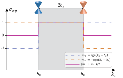
Figure S1: Hall conductivity of a theory with two Weyl cones separated in the $k_{z}$ direction. For each $k_{z}$, the theory is equivalent to two 2+1-dimensional gapped Dirac theories with $k_{z}$-dependent masses (dashed lines). The total 3D Hall conductivity is the integral of the solid curve, and is proportional to the Weyl node separation, see Eq. (73).

Appendix C Consistency with the 2+1-dimensional fermionic duality

We start by reminding the reader that the Weyl semimetal theory Eq. (55), that we repeat here for convenience

$$S_{b} = \int d^{4}x\bar{\psi}\gamma^{\mu}(\partial_{\mu}+iA_{\mu}+ib_{\mu}\gamma_{5})\psi,$$ (71)

can be viewed as layered 2+1-dimensional Dirac theories. Consider the case when the Weyl node separation is space-like and along the $\hat{z}$ direction. This is equivalent to choosing $b^{\mu}=(0,\mathbf{b})$. Further choosing $\mathbf{b}\parallel\hat{z}$ simplifies our discussion but does not affect the generality of our conclusions. We observe that we can decompose this theory into a sum over two 2+1-dimensional massive Dirac equations. Fourier transforming to momentum space along $\mathbf{b}$ we obtain

$$S = \int d^{4}x\,\left[\bar{\psi}_{L}\,\sigma^{\mu}_{L,\parallel}(\partial_{\mu,\parallel}+iA_{\mu,\parallel})+\sigma_{z}(k_{z}+A_{z}+b_{z}))\psi_{L}\right.$$ (72)

$$+ \left.\bar{\psi}_{R}\,(\sigma^{\mu}_{R,\parallel}\left(\partial_{\mu}+iA_{\mu,\parallel}\right)-\sigma_{z}(k_{z}+A_{z}-b_{z}))\psi_{R}\right].$$

When $A_{\mu}=0$, the terms $\pm\sigma_{z}(k_{z}\pm b_{z})$ act as a mass term for 2+1-dimensional Dirac fermions parametrized by $k_{z}$ with masses $m_{\pm}=(\pm k_{z}+b_{z})$. When $k_{z}=b_{z}$ ($k_{z}=-b_{z}$), $m_{-}=0$ ($m_{+}=0$) the gap corresponding to chirality $R$ ($L$) closes, setting the location of the 3+1 dimensional $R$ ($L$) Weyl node.

When $A_{\mu}\neq 0$, a gapped 2+1-dimensional Dirac system with mass $m$ responds with a Hall conductivity $\sigma^{(2D)}_{xy}$ proportional to the sign of its mass, such that $\sigma^{(2D)}_{xy}=\mathrm{sign}(m)e^{2}/2h$. Depending on the value of $k_{z}$, the Hall conductivity of the Dirac fermions that compose the Weyl semimetal can either add up or cancel each other (see Fig. S1), resulting in a Hall effect proportional to the Weyl node separation Burkov and Balents (2011); Zyuzin et al. (2012); Grushin (2012); Zyuzin and Burkov (2012); Goswami and Tewari (2013):

$$\sigma^{(3D)}_{xy} = \int\dfrac{dk_{z}}{2\pi}\dfrac{e^{2}}{h}[\mathrm{sign}(k_{z}+b_{z})-\mathrm{sign}(k_{z}-b_{z})]$$ (73)

$$= \dfrac{e^{2}}{2h}\dfrac{2b_{z}}{2\pi}.$$

This coincides with the current response derived from Eq. (56) which we repeat here for convenience (in Minkowski space):

$$S_{b} = -\dfrac{1}{4\pi^{2}}\int d^{4}x\,\epsilon^{\mu\nu\rho\sigma}b_{\mu}A_{\nu}\partial_{\rho}A_{\sigma}.$$ (74)

In Son’s 2+1-dimensional duality, a Dirac mass $m$ on one side of the duality maps to $-m$ in the dual theory Metlitski and Vishwanath (2016); Sachdev . This means that if our duality is to be correct, we should recover the Hall conductivity resulting from the masses $-m_{\pm}=(\mp k_{z}-b_{z})$. In this case we should recover a Hall conductivity given by

$$\sigma^{(3D)}_{\mathrm{dual},xy} = \int\dfrac{dk_{z}}{2\pi}\dfrac{e^{2}}{h}[-\mathrm{sign}(k_{z}+b_{z})+\mathrm{sign}(k_{z}-b_{z})]$$ (75)

$$= -\dfrac{e^{2}}{2h}\dfrac{2b_{z}}{2\pi}.$$

In the main text, we showed that for our Weyl duality to hold, $b_{\mu}$ must map to $-b_{\mu}$, which is exactly the difference between Eqs. (73) and (75). Hence, our Weyl duality passes this consistency check implied by Son’s duality.

References

- Amorim et al. (2016) B. Amorim, A. Cortijo, F. de Juan, A. Grushin, F. Guinea, A. Gutiérrez-Rubio, H. Ochoa, V. Parente, R. Roldán, P. San-Jose, J. Schiefele, M. Sturla, and M. Vozmediano, Physics Reports 617, 1 (2016), novel effects of strains in graphene and other two dimensional materials.
- Ilan et al. (2020) R. Ilan, A. G. Grushin, and D. I. Pikulin, Nature Reviews Physics 2, 29 (2020).
- Kharzeev (2015) D. E. Kharzeev, Annual Review of Nuclear and Particle Science 65, 193 (2015).
- Bertlmann (1996) R. A. Bertlmann, Anomalies in Quantum Field Theories (Clarendon, Oxford, UK, 1996).
- Armitage et al. (2018) N. P. Armitage, E. J. Mele, and A. Vishwanath, Rev. Mod. Phys. 90, 015001 (2018).
- Fukushima et al. (2008) K. Fukushima, D. E. Kharzeev, and H. J. Warringa, Phys. Rev. D 78, 074033 (2008).
- Savit (1980) R. Savit, Rev. Mod. Phys. 52, 453 (1980).
- Son (2015) D. T. Son, Physical Review X 5, 031027 (2015).
- Senthil et al. (2019) T. Senthil, D. T. Son, C. Wang, and C. Xu, Physics Reports 827, 1 (2019).
- Peskin (1978) M. E. Peskin, Elsevier 113, 122 (1978).
- Dasgupta and Halperin (1981) C. Dasgupta and B. I. Halperin, Phys. Rev. Lett. 47, 1556 (1981).
- Mross et al. (2016) D. F. Mross, J. Alicea, and O. I. Motrunich, Phys. Rev. Lett. 117, 016802 (2016).
- Metlitski and Vishwanath (2016) M. A. Metlitski and A. Vishwanath, Phys. Rev. B 93, 245151 (2016).
- Wang and Senthil (2015) C. Wang and T. Senthil, Phys. Rev. X 5, 041031 (2015).
- Seiberg et al. (2016) N. Seiberg, T. Senthil, C. Wang, and E. Witten, Annals of Physics 374, 395 (2016).
- Karch and Tong (2016) A. Karch and D. Tong, Phys. Rev. X 6, 031043 (2016).
- Benini (2018) F. Benini, Journal of High Energy Physics 2018, 68 (2018).
- Murugan and Nastase (2017) J. Murugan and H. Nastase, Journal of High Energy Physics 2017, 1 (2017).
- Xu and You (2015) C. Xu and Y.-Z. You, Phys. Rev. B 92, 220416 (2015).
- Sodemann et al. (2017) I. Sodemann, I. Kimchi, C. Wang, and T. Senthil, Phys. Rev. B 95, 085135 (2017).
- Jensen and Patil (2019) K. Jensen and P. Patil, Journal of High Energy Physics 2019, 129 (2019).
- Chen and Zimet (2018) J.-Y. Chen and M. Zimet, Journal of High Energy Physics 2018, 1 (2018).
- Potter et al. (2017) A. C. Potter, C. Wang, M. A. Metlitski, and A. Vishwanath, Phys. Rev. B 96, 235114 (2017).
- Sagi et al. (2018) E. Sagi, A. Stern, and D. F. Mross, Phys. Rev. B 98, 201111 (2018).
- Palumbo (2020) G. Palumbo, Annals of Physics 419, 168240 (2020).
- Bi and Senthil (2019) Z. Bi and T. Senthil, Phys. Rev. X 9, 021034 (2019).
- Wan and Wang (2019) Z. Wan and J. Wang, Phys. Rev. D 99, 065013 (2019).
- Furusawa and Nishida (2019) T. Furusawa and Y. Nishida, Phys. Rev. D 99, 101701 (2019).
- Niemi and Semenoff (1983) A. J. Niemi and G. W. Semenoff, Physical Review Letters 51, 2077 (1983).
- Burkov (2019) A. A. Burkov, Phys. Rev. B 99, 035124 (2019).
- Li et al. (2013) Y. Li, S.-C. Zhang, and C. Wu, Phys. Rev. Lett. 111, 186803 (2013).
- Note (1) A note on wording: throughout our work we avoid the terminology of chiral gauge fields in favour of axial gauge fields to collectively refer to fields that couple with opposite signs to different helicities in 2+1 dimensions, or chiralities in 3+1 dimensions, since chirality is only well defined in even space-time dimensions.
- Cortijo et al. (2010) A. Cortijo, A. G. Grushin, and M. A. H. Vozmediano, Phys. Rev. B 82, 195438 (2010).
- Wieder et al. (2018) B. J. Wieder, B. Bradlyn, Z. Wang, J. Cano, Y. Kim, H.-S. D. Kim, A. M. Rappe, C. L. Kane, and B. A. Bernevig, Science 361, 246 (2018).
- Kalb and Ramond (1974) M. Kalb and P. Ramond, Phys. Rev. D 9, 2273 (1974).
- Banks and Seiberg (2011) T. Banks and N. Seiberg, Phys. Rev. D 83, 084019 (2011).
- Cho and Moore (2011) G. Y. Cho and J. E. Moore, Annals of Physics 326, 1515 (2011).
- Chan et al. (2013) A. Chan, T. L. Hughes, S. Ryu, and E. Fradkin, Phys. Rev. B 87, 085132 (2013).
- Cirio et al. (2014) M. Cirio, G. Palumbo, and J. K. Pachos, Phys. Rev. B 90, 085114 (2014).
- Maciejko et al. (2014) J. Maciejko, V. Chua, and G. A. Fiete, Phys. Rev. Lett. 112, 016404 (2014).
- Putrov et al. (2017) P. Putrov, J. Wang, and S. T. Yau, Annals of Physics 384, 254 (2017).
- Ramamurthy and Hughes (2015) S. T. Ramamurthy and T. L. Hughes, Phys. Rev. B 92, 085105 (2015).
- Galeski et al. (2020) S. Galeski, X. Zhao, R. Wawrzyńczak, T. Meng, T. Förster, S. Honnali, N. Lamba, T. Ehmcke, A. Markou, W. Zhu, J. Wosnitza, C. Felser, G. F. Chen, and J. Gooth, arXiv e-prints , arXiv:2003.07213 (2020), arXiv:2003.07213 [cond-mat.str-el] .
- Thakurathi and Burkov (2020) M. Thakurathi and A. A. Burkov, Phys. Rev. B 101, 235168 (2020).
- Wan et al. (2011) X. Wan, A. M. Turner, A. Vishwanath, and S. Y. Savrasov, Phys. Rev. B 83, 205101 (2011).
- Zyuzin and Burkov (2012) A. A. Zyuzin and A. A. Burkov, Phys. Rev. B 86, 115133 (2012).
- Grushin (2012) A. G. Grushin, Phys. Rev. D 86, 045001 (2012).
- Zyuzin et al. (2012) A. A. Zyuzin, S. Wu, and A. A. Burkov, Physical Review B 85, 165110 (2012).
- Goswami and Tewari (2013) P. Goswami and S. Tewari, Phys. Rev. B 88, 245107 (2013).
- Colladay and Kostelecký (1997) D. Colladay and V. A. Kostelecký, Phys. Rev. D 55, 6760 (1997).
- Colladay and Kostelecký (1998) D. Colladay and V. A. Kostelecký, Phys. Rev. D 58, 116002 (1998).
- Carroll et al. (1990) S. M. Carroll, G. B. Field, and R. Jackiw, Phys. Rev. D 41, 1231 (1990).
- de Juan et al. (2017) F. de Juan, A. G. Grushin, T. Morimoto, and J. E. Moore, Nature Communications 8 (2017), doi:10.1038/ncomms15995.
- Avdoshkin et al. (2020) A. Avdoshkin, V. Kozii, and J. E. Moore, Phys. Rev. Lett. 124, 196603 (2020).
- Florens and Georges (2002) S. Florens and A. Georges, Phys. Rev. B 66, 165111 (2002).
- Florens and Georges (2004) S. Florens and A. Georges, Phys. Rev. B 70, 035114 (2004).
- Burkov and Balents (2011) A. A. Burkov and L. Balents, Phys. Rev. Lett. 107, 127205 (2011).
- Hermele (2007) M. Hermele, Phys. Rev. B 76, 035125 (2007).
- Xu (2010) C. Xu, Phys. Rev. B 81, 144431 (2010).
- Pesin and Balents (2010) D. Pesin and L. Balents, Nature Physics 6, 376 (2010).
- Lee and Lee (2005) S.-S. Lee and P. A. Lee, Physical Review Letters 95, 1196 (2005).
- Barkeshli and McGreevy (2012) M. Barkeshli and J. McGreevy, Physical Review B 86, 075136 (2012).
- Villain, J. (1975) Villain, J., J. Phys. France 36, 581 (1975).
- Agarwal (2019) A. Agarwal, Physical Review Letters 123, 211601 (2019).
- (65) S. Sachdev, Boson-fermion and fermion-fermion dualities.
- Goswami and Roy (2012) P. Goswami and B. Roy, arXiv e-prints , arXiv:1211.4023 (2012), arXiv:1211.4023 [cond-mat.mes-hall] .
- Behrends et al. (2019) J. Behrends, S. Roy, M. H. Kolodrubetz, J. H. Bardarson, and A. G. Grushin, Phys. Rev. B 99, 140201 (2019).
- Vazifeh and Franz (2013) M. M. Vazifeh and M. Franz, Phys. Rev. Lett. 111, 027201 (2013).
- Grushin et al. (2015) A. G. Grushin, J. W. F. Venderbos, and J. H. Bardarson, Phys. Rev. B 91, 121109 (2015).
- Fujikawa (1984) K. Fujikawa, Phys. Rev. D 29, 285 (1984).
- Chung (1999) J.-M. Chung, Phys. Rev. D 60, 127901 (1999).
- Seradjeh and Franz (2008) B. Seradjeh and M. Franz, Phys. Rev. Lett. 101, 146401 (2008).
- Marzuoli and Palumbo (2012) A. Marzuoli and G. Palumbo, EPL (Europhysics Letters) 99, 10002 (2012).
- Hasan and Kane (2010) M. Z. Hasan and C. L. Kane, Rev. Mod. Phys. 82, 3045 (2010).
- Chang et al. (2017) G. Chang, S.-Y. Xu, B. J. Wieder, D. S. Sanchez, S.-M. Huang, I. Belopolski, T.-R. Chang, S. Zhang, A. Bansil, H. Lin, and M. Z. Hasan, Phys. Rev. Lett. 119, 206401 (2017).
- Flicker et al. (2018) F. Flicker, F. de Juan, B. Bradlyn, T. Morimoto, M. G. Vergniory, and A. G. Grushin, Phys. Rev. B 98, 155145 (2018).
- Meng (2015) T. Meng, Phys. Rev. B 92, 115152 (2015).
- Levin and Fisher (2009) M. Levin and M. P. A. Fisher, Phys. Rev. B 79, 235315 (2009).
- Burkov et al. (2011) A. A. Burkov, M. D. Hook, and L. Balents, Phys. Rev. B 84, 235126 (2011).
- Metlitski et al. (2017) M. A. Metlitski, A. Vishwanath, and C. Xu, Phys. Rev. B 95, 205137 (2017).
- Jian et al. (2019) C.-M. Jian, Z. Bi, and Y.-Z. You, Phys. Rev. B 100, 075109 (2019).
- Hsin and Seiberg (2016) P.-S. Hsin and N. Seiberg, Journal of High Energy Physics 2016, 95 (2016).
- Aharony et al. (2017) O. Aharony, F. Benini, P.-S. Hsin, and N. Seiberg, Journal of High Energy Physics 2017, 72 (2017).
- Argurio et al. (2019) R. Argurio, M. Bertolini, F. Mignosa, and P. Niro, Journal of High Energy Physics 2019, 153 (2019).
- Mañes (2012) J. L. Mañes, Physical Review B 85, 155118 (2012).
- Bradlyn et al. (2016) B. Bradlyn, J. Cano, Z. Wang, M. Vergniory, C. Felser, R. J. Cava, and B. A. Bernevig, Science 353, aaf5037 (2016).
- Wieder et al. (2016) B. J. Wieder, Y. Kim, A. Rappe, and C. Kane, Physical review letters 116, 186402 (2016).
- Tang et al. (2017) P. Tang, Q. Zhou, and S.-C. Zhang, Phys. Rev. Lett. 119, 206402 (2017).
- Chang et al. (2018) G. Chang, B. J. Wieder, F. Schindler, D. S. Sanchez, I. Belopolski, S.-M. Huang, B. Singh, D. Wu, T.-R. Chang, T. Neupert, et al., Nature materials 17, 978 (2018).
- Zhu et al. (2020) Y.-Q. Zhu, N. Goldman, and G. Palumbo, arXiv e-prints , arXiv:2006.00170 (2020), arXiv:2006.00170 [cond-mat.mes-hall] .
- Deser et al. (1982) S. Deser, R. Jackiw, and S. Templeton, Annals of Physics 140, 372 (1982).