The Home Office in Times of COVID- 19 Pandemic and its impact in the Labor Supply

Abstract

We lightly modify Eriksson’s (1996) model to accommodate the home office in a simple model of endogenous growth. By home office we mean any working activity carried out away from the workplace which is assumed to be fixed. Due to the strong mobility restrictions imposed on citizens during the COVID-19 pandemic, we allow the home office to be located at home. At the home office, however, in consequence of the fear and anxiety workers feel because of COVID-19, they become distracted and spend less time working.

We show that in the long run, the intertemporal elasticity of substitution of the home- office labor is sufficiently small only if the intertemporal elasticity of substitution of the time spent on distracting activities is small enough also.

Keywords: COVID-19; Social Distancing; Home Office; Economic growth model.
JEL Codes: O41.

1 Introduction

The home office is a modality of working away from a fixed job location the office and therefore can be carried out in any place different from a physical office. This modality of labor has existed for a long time and has been mainly common in multinational enterprises. However, this modality of working has increased over time around the world as shown in a survey carried out by Ipsos, see Fig. 1 below.

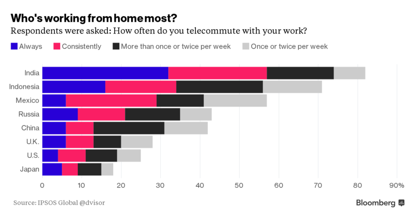
Figure 1: India, Indonesia and Mexico had the highest amount of telecommuters.

In spite of the significant gains from working from home in terms of worker productivity and satisfaction as shown in Bloom et al. (2015), it does not seem to be the case during the COVID-19 pandemic, as workers could engage in distracting activities placing workers’ productivity at risk. In this same vein of reasoning, Dutcher and Jabs Saral (2012) highlight, even in normal times, the difficulties that may arise if telecommuting workers are not properly monitored.

In spite of the fact that the home office or working from home in the past it was only applied to specific jobs, nowadays, because the COVID-19 pandemic, most firms seem to be obligated to adopt it to continue operating in their markets. Consequently, both the demand and supply for home offices seem to increase. Hence, it is the purpose of this paper to theoretically determine the factors which influence the home-office job supply.

Of course not all jobs can be accomplished in a remote way This makes the productive sector seek to reorganise itself so that working from home becomes the best alternative due to the strong mobility restrictions imposed by the authorities of countries. It is also well known that many enterprises are planning on adopting home offices even after the current pandemic. So much so, that in many countries some businesses, like hotels, are planning to adapt their spaces to offer them as places to set up home offices. This obliges us to make a long-run analysis of the home-office job supply.

To accomplish our purpose we consider a simple economic growth model with an endogenous labor supply like that of Eriksson (1996). Although our model is very similar to Eriksson?s model, we depart from it in the following aspect. We assume that the effort attached to human capital depends on the time spent on distracting activities, occurring during the working period. We assume that these distracting activities give some pleasure to workers, but we should not confuse such activities with leisure activities since the latter are supposed to occur outside normal working hours.

It is also useful to note that during the COVID-19 pandemic, workers are put on quarantine. It is therefore natural to assume that workers are more prone to be distracted by activities that decrease their home office production. We can interpret such distracting activities as being negative “shocks” to the labor supply. The word shock used here is not used in its rigorous sense of being stochastic since the economic growth model we used here is deterministic.

Our paper is related to the recent literature on the economic effects of the COVID-19 crisis. The papers in this literature have different objectives - from understanding its evolution to predicting its impacts on the world economy. Nonetheless, our paper is more related to the working-from-home literature which is surveyed by Allen et al. (2015). These authors address a type of home office, namely telecommuting and analyse how effective it is.

Our objective in this paper is much more modest in the sense that we seek to discover how the preferences for consumption and displeasure for working affect the growth of home- office job supply. More precisely, we show that this growth rate is affected by the parameters that represent both the workers? preferences for consumption and the workers? displeasure for working. This is important for both firms and governments as it allows them to implement, in an optimal way, the incentives for home-office job supply by adjusting the goals of each policy maker. Our specific findings are related to the growth rate of variables along balanced-growth solution paths. We show that in the long run the intertemporal elasticity of substitution of home-office labor is sufficiently small only if the intertemporal elasticity of substitution of the time spent on distracting activities is small enough too.

The paper is organised as follows: Section 2 presents the model in which are described both households and firms. In this same section, the social planner?s problem is formulated. Section 3 presents the main results and the paper ends with a short section which analyses the theoretical results and gives some concluding remarks.

2 The model

Our model is a centralised economy like that of Eriksson (1996) with some key modifications allowing us to make the labor supply endogenous via distracting activities. By distracting activities here I mean any activity which decreases labor time. They are not properly leisure but rather activities which produce both pleasure and affect or influence the acquisition of human capital which is placed in motion to produce consumption good/capital.

Remark 1

Distracting activities influence the effort which is allocated to produce either consumption goods or capital for future investments. Moreover, these activities also influence the effort used to acquire human capital.

2.1 Households

We allow each worker, within a constant population, to supply labor $l_{t}.$ We assume that during the working hours each worker spends time $s_{t}$ in distracting activities which give a certain pleasure. It is useful to pointing out that the time $s_{t}$ is not leisure since it occurs during working hours $l_{t}.$ Thus, $l_{s}-s_{t}$ is the effective labor.

We model the instantaneous payoff of each worker to be

$$V(c_{t},s_{t},l_{t})=u(c_{t})-v(l_{t}-s_{t})$$

This payoff consists of two parts: the former is the pleasure coming from consumption and the latter is the displeasure felt while working.

2.2 Production

On the production side of the economy, the output is produced by using both capital, $k_{t}$ and effective labor $l_{t}-s_{t}$ which is potentiated by the human capital $h_{t}.$ We formalise this by assuming the effort depends on $s_{t}.$

Differently from Uzawa (1965) and Lucas (1988), we make human capital endogenous by postulating each worker’s effort $e:[0,l_{t}]\to[0,1]$ depends on the time spent $s_{t}$ in the following way: $e(s_{t})=1-\frac{s_{t}}{l_{t}}.$ We also assume that this effort is allocated both to the production of human capital and the consumption good/capital. Our allocation is $(1-e)$ for the former and $e$ for the latter. More precisely, we assume that both human and physical (or real) capitals accumulate according to

$$\dot{h}_{t}=h_{t}(1-e(s_{t}))$$

$$\dot{k}_{t}=f(k_{t},h_{t}e(s_{t})(l_{t}-s_{t}))-c_{t}$$

respectively. Using the functional form of $e,$ we can rewrite (1) and (2) to be

$$\dot{h}_{t}=h_{t}\frac{s_{t}}{l_{t}}$$

$$\dot{k}_{t}=f(k_{t},\frac{h_{t}}{l_{t}}(l_{t}-s_{t})^{2})-c_{t}$$

2.3 The planner

After describing the consumption and production sides, we are going to formulate the benevolent planner’s problem. The benevolent planner’s problem is then to chose paths of consumption $c,$ labor $l,$ and time spent $s$ on distracting activities in order to maximise the discounted stream of payoffs by every identical agent in the economy

$$\int_{0}^{\infty}e^{-\rho t}V(c_{t},l_{t},s_{t})dt$$

subject to (3) and (4) with $k_{o}>0$ and $h_{o}>$ given.

Here, $c_{t},l_{t}$ and $s_{t}$ are control variables and $\rho$ is the discount factor; and $k_{t}$ and $h_{t}$ are state variables. In what follows we will drop all indexes of time from variables which depend on the time to attain analytical tractability.

In this model the effort $e$ is endogenous, not by itself, like Eriksson (1996), but because it depends on the time spent on distracting activities. However, for the sake of comparison with related literature and mainly with that of Eriksson’s (1996) paper, we maintain, like him, that the instantaneous payoff is additively separable:

$$V(c,s,l)=\frac{c^{1-\sigma}}{1-\sigma}-\frac{(l-s)^{1+\gamma}}{1+\gamma},1\not=\sigma>0,\gamma>0,$$

and the production function like a Cobb-Douglas one :

$$f(k,he(l-s))=k^{\beta}[\frac{h}{l}(l-s)^{2}]^{1-\beta}.$$

3 Theoretical results

We begin this section by characterising the solutions of the benevolent planner?s problem. For that, we consider the current-value Hamiltonian for the optimal problem, with “prices” $\lambda_{1}$ and $\lambda_{2}$ used to value increments to physical and human capital respectively.

$$H=\frac{c^{1-\sigma}}{1-\sigma}-\frac{(l-s)^{1+\gamma}}{1+\gamma}+\lambda_{1}[k^{\beta}[\frac{h}{l}(l-s)^{2}]^{1-\beta}-c]+\lambda_{2}h\frac{s}{l}.$$

The necessary conditions for optimality are:

1. $$H_{c}=0\Leftrightarrow c^{-\sigma}=\lambda_{1}$$

2. $$H_{s}=0\Leftrightarrow(l-s)^{\gamma}+(1-\beta)\lambda_{1}k^{\beta}[\frac{h}{l}(l-s)^{2}]^{-\beta}h(-2+\frac{2s}{l})+\lambda_{2}\frac{h}{l}=0$$

3. $$H_{l}=0\Leftrightarrow-(l-s)^{\gamma}+\lambda_{1}(1-\beta)k^{\beta}[\frac{h}{l}(l-s)^{2}]^{-\beta}h(1-\frac{s^{2}}{l^{2}})-\lambda_{2}h\frac{s}{l^{2}}=0$$

4. $$\dot{\lambda}_{1}=\rho\lambda_{1}-H_{k}$$

   $$\Updownarrow$$

   $$\dot{\lambda}_{1}=\lambda_{1}\{\rho-\beta k^{\beta-1}[\frac{h}{l}(l-s)^{2}]^{1-\beta}\}.$$

5. $$\dot{\lambda}_{2}=\rho\lambda_{2}-H_{h}$$

   $$\Updownarrow$$

   $$\dot{\lambda}_{2}=\lambda_{2}\rho-\lambda_{1}(1-\beta)k^{\beta}[\frac{h}{l}(l-s)^{2}]^{-\beta}\frac{(l-s)^{2}}{l}-\lambda_{2}\frac{s}{l}$$

(8) -(10 ) are the the first order conditions to to maximise $H,$ and (11) and (12) give the rates of change of $\lambda_{i},i=1,2$ of both capitals.

3.1 Steady state path

Next, we will seek the balanced growth path from (8)-(12) which are solutions on which consumption and both kinds of capital are growing at constant percentage rates, the prices of the two kinds of capital are declining at constant rates.

In what follows we will present our first results which have to do with the relationships between the rates of change of our variables $k,c,l-s$ and $h.$

Proposition 1

Along the balanced growth solution of the planner’s problem, we have

$$\hat{k}=\hat{c}=\hat{h}+2\hat{(l-s)}-\hat{l}$$

Proof.

From (8) we have $\hat{\lambda}_{1}=-\sigma\hat{c}.$ So that if $\hat{c}=\theta,$ then from (11) we get that the marginal productivity of capital is constant. That is,

$$k^{\beta-1}[\frac{h}{l}(l-s)^{2}]^{1-\beta}=\frac{\rho+\sigma\theta}{\beta}.$$

Dividing by $k$ through (4) and using (7), we have

$$\frac{c}{k}=k^{\beta-1}[\frac{h}{l}(l-s)^{2}]^{1-\beta}-\hat{k}$$

Using (13) and the fact that $\hat{k}$ grows at a constant rate, by hypothesis, one has $\frac{c}{k}$ is a constant. After Differentiating (14) logarithmically with respect to time we get

$$\hat{k}=\hat{c}=\theta.$$

Differentiating (13) logarithmically with respect to time one has that the common growth rate of consumption and capital is

$$\theta=\hat{h}+2\hat{(l-s)}-\hat{l}$$

 

Proposition 2

Under the same hypotheses of Proposition 1, one has:

1. $\hat{s}=\hat{l}=\hat{(l-s)}=\frac{1-\sigma}{\gamma+\sigma}\hat{h}$

2. $\hat{k}=\hat{c}=\frac{1+\gamma}{\gamma+\sigma}\hat{h}$

Proof.

Summing (9) and (10) we get

$$(1-\beta)k^{\beta}[\frac{h}{l}(l-s)^{2}]^{-\beta}\frac{\lambda_{1}}{\lambda_{2}}(l-s)=1$$

Differentiating (17) logarithmically with respect to time and using (15) and (8) one has

$$\hat{\lambda}_{2}=(1-\beta)\hat{(l-s)}-\beta\hat{h}+(\beta-\sigma)\theta$$

Manipulating (9) and (17) we have

$$(l-s)^{\gamma}=2\frac{h\lambda_{2}}{l}$$

Differentiating (19) logarithmically with respect to time we have

$$\gamma\hat{(l-s)}=\hat{\lambda}_{2}+\hat{h}-\hat{l}$$

Manipulating (12) and using (17) we have $\hat{l-s}=\hat{l}.$ Using this fact, (16) and (20) become

$$\theta=\hat{h}+\hat{(l-s)}$$

$$(\gamma+1)\hat{(l-s)}=\hat{\lambda}_{2}+\hat{h}$$

respectively.

Putting (18) and (21) into (22) and after arranging it we have.

$$\hat{(l-s)}=\frac{1-\sigma}{\gamma+\sigma}\hat{h}$$

Since $\hat{h}$ is constant we have that $\hat{l}=\hat{s}$ by (3). Using the fact that $\hat{l-s}=\hat{l},$ stablished above, we get Item 1. Putting (23) into (21) we get

$$\theta=\hat{h}+\frac{1-\sigma}{\gamma+\sigma}\hat{h}=(1+\frac{1-\sigma}{\gamma+\sigma})\hat{h}$$

Hence, Item 2 follows.

 

The following proposition shows that the growth rates in terms of parameters.

Proposition 3

Under the same hypotheses of Proposition 1, one has:

1. $\hat{s}=\hat{l}=\hat{(l-s)}=\frac{(1-\sigma)(\rho-1)}{1-\sigma(2+\gamma)}$

2. $\hat{k}=\hat{c}=\frac{(1+\gamma)(\rho-1)}{1-\sigma(2+\gamma)}$

Proof.

After manipulating (12) and to use (17) and (3) we reach to

$$\hat{\lambda}_{2}=\rho-1$$

Putting (25) into (22) one has

$$(1+\gamma)\hat{(l-s)}=\rho-1+\hat{h}$$

Putting (21) into (26) we have

$$(1+\gamma)\theta=(2+\gamma)\hat{h}+\rho-1$$

Putting (24) into (27) and after simplifying the result we get

$$\hat{h}=\frac{(\gamma+\sigma)(\rho-1)}{1-\sigma(2+\gamma)}$$

Finally, Proposition 3 follows after substituting (28) into Items 1 and 2 of Proposition 2.

 

The following corollary shows the growth rate of the output equals the growth rate of the capital (or consumption).

Corollary 1

Under assumptions of Proposition 3, one has

$$\hat{y}=\hat{k}=\hat{c}$$

Proof. This result follows from Differentiating (7) logarithmically with respect to time and using (16) and Item 2 of Proposition 3.   

3.2 Convergent utility and transversality conditions

In this section, we establish the convergence of the utility function and the transversality condition. We will do it by considering the balanced path and under the assumption that $\sigma>1.$

First, the utility integral can be written as

$$U=A_{1}\int_{0}^{\infty}e^{((1-\sigma)\hat{c}-\rho)t}dt-A_{2}\int_{0}^{\infty}e^{((1+\gamma)\hat{(l-s)}-\rho)t}dt$$

where $A_{1}=\frac{c_{o}^{1-\sigma}}{1-\sigma}$ and $A_{1}=\frac{(l_{o}-s_{o})^{1+\gamma}}{1+\gamma}.$ Substituting the values of $\hat{c}$ and $\hat{l-s}$ given by Proposition 3 we have that $U$ is

$$U=(A_{1}-A_{2})\int_{0}^{\infty}e^{xt}dt$$

where $x=\frac{(1+\gamma)(1-\sigma)(\rho-1)}{1-\sigma(2+\gamma)}-\rho$ is negative since $\sigma>1$ and $\rho<1.$ Thus, $U$ is finite since $x$ is negative.

Second, the transversality conditions associated with the benevolent planner’s problem also hold. That is to say,

$$\lim_{t\to\infty}k\lambda_{1}e^{-\rho t}=0\hbox{ and }\lim_{t\to\infty}h\lambda_{2}e^{-\rho t}=0$$

The former follows from the facts $\hat{\lambda}_{1}=-\sigma\hat{c}$ and $\hat{k}=\hat{c}.$ Thus, one has

$$k\lambda_{1}e^{-\rho t}=k_{o}(\lambda_{1})_{o}e^{(\hat{k}-\sigma\hat{c})t}=k_{o}(\lambda_{1})_{0}e^{[(1-\sigma)\hat{c}-\rho]t}$$

Since $(1-\sigma)\hat{c}-\rho=x$ and $x$ is negative from its definition (see above), the former result follows.

Finally, the latter follows from (25) and (28). To see it, it suffice to observe that

$$h\lambda_{2}e^{-\rho t}=h_{o}(\lambda_{2})_{o}e^{(\hat{h}+\hat{\lambda}_{2}-\rho)t}$$

where $\hat{h}+\hat{\lambda}_{1}-\rho$ equals $x.$ Since $x$ is negative, the latter result follows.

3.3 The intertemporal elasticity of distracting activities

We start by setting the elasticity of the marginal utility of time spent on distracting activities, $V_{2}(c_{t},s_{t},l_{t}).$ Here the sub-index represents the partial derivative with respect to $s_{t}.$

By definition of elasticity one has

$${\cal E}_{V}(s_{t})=\frac{\partial V_{2}}{\partial s_{t}}\frac{s_{t}}{V_{2}}$$

Using (6) we compute ${\cal E}_{V}(s_{t}).$ Thus,

$${\cal E}_{V}(s_{t})=\gamma\frac{s_{t}}{l_{t}-s_{t}}$$

Manipulating and using (3) we get

$${\cal E}_{V}(s_{t})=\gamma\frac{\hat{h}}{1-\hat{h}}$$

Considering again the balanced path and using (28) we write ${\cal E}_{V}(s_{t})$ in terms of parameters

$${\cal E}_{V}(s_{t})=\gamma\frac{\frac{(\gamma+\sigma)(\rho-1)}{1-\sigma(2+\gamma)}}{1-\frac{(\gamma+\sigma)(\rho-1)}{1-\sigma(2+\gamma)}}$$

We know that the intertemporal elasticity of substitution of time spent on distracting activities $IES$ is defined as $\frac{1}{{\cal E}_{V}(s_{t})}$ so that

$$IES(s)=\frac{(1+\gamma)(1-\sigma)-\rho(\gamma+\sigma)}{\gamma(\gamma+\sigma)(\rho-1)}$$

For $\sigma>1$ and $\rho<1,$ we clearly have that $IES(s)$ tends to 0 as $\gamma\to\infty.$

4 Analysis of results and concluding remarks

First, in relation to the home-office job supply represented by $l_{t}-s_{t}$ we know from (6) that the intertemporal elasticity of substitution of the home office is $\frac{1}{\gamma}$ and the intertemporal elasticity of substitution of consumption is $\frac{1}{\sigma}.$ Second, for the balanced growth path satisfying (8) - (12) to be a solution of the benevolent planner’s problem it is sufficient that the transversality conditions are satisfied. This is achieved by assuming $\sigma>1.$ Third, differently from Eriksson’s (1996) model we have considered the productivity of human capital sector as being 1 and the discount factor $\rho<1.$ Lastly, if workers had been patients ( $\rho=1$), we would have considered the productivity of the human capital sector as being greater than 1 in order to keep the results similar to that of Eriksson as is shown in Propositions 2, 3 and Corollary 1.

Using all the results of the previous paragraph, we can then say that the intertemporal elasticity of substitution of time spent on distracting activities, $IES(s)$ is small enough provided that the intertemporal elasticity of substitution of home-office is small enough. More precisely one has that

$$\lim_{\gamma\to\infty}IES(s)=0$$

The intuition behind this result is that if workers want to avoid fluctuations in home-office labor, they should display strong preference to avoid fluctuations on distracting activities. This result does not seem to be plausible in the short-run due to the high volatility of the distracting activities because of the COVID-19 pandemic that has spread throughout the world provoking fear and anxiety in citizens and particularly in workers. However, to have $IES(s)$ small enough does seem to be quite plausible in the long-run since workers will end up incorporating home office work if it is adopted as a form of labor.

We finish this section by saying that although our paper is deterministic, it does explain to a certain degree, the long-run behaviour of the home-office job supply in terms of time spent on distracting activities. More precisely, a necessary condition for the home-office job supply to be smooth is that the intertemporal elasticity of substitution of distracting activities be small enough, as shown in the previous limit. We hope that in future research the home-office job supply will be analysed in ampler settings, including markets and government.