INT: An Inequality Benchmark for Evaluating Generalization in Theorem Proving

Abstract

In learning-assisted theorem proving, one of the most critical challenges is to generalize to theorems unlike those seen at training time. In this paper, we introduce INT, an INequality Theorem proving benchmark designed to test agents’ generalization ability. INT is based on a theorem generator, which provides theoretically infinite data and allows us to measure 6 different types of generalization, each reflecting a distinct challenge, characteristic of automated theorem proving. In addition, INT provides a fast theorem proving environment with sequence-based and graph-based interfaces, conducive to performing learning-based research. We introduce baselines with architectures including transformers and graph neural networks (GNNs) for INT. Using INT, we find that transformer-based agents achieve stronger test performance for most of the generalization tasks, despite having much larger out-of-distribution generalization gaps than GNNs. We further find that the addition of Monte Carlo Tree Search (MCTS) at test time helps to prove new theorems.

1 Introduction

Advances in theorem proving can catalyze developments in fields including formal mathematics (McCune, 1997), software verification (Darvas et al., 2005), and hardware design (Kern and Greenstreet, 1999). Following its recent success across other application domains, machine learning has significantly improved the performance of theorem provers (Bansal et al., 2019; Bridge et al., 2014; Gauthier et al., 2018; Huang et al., 2019; Irving et al., 2016; Kaliszyk et al., 2018; Lee et al., 2020; Loos et al., 2017; Urban et al., 2011; Wang and Deng, 2020; Yang and Deng, 2019; Li et al., 2020; Rabe et al., 2020; Polu and Sutskever, 2020). Two key factors that make theorem proving particularly challenging for ML are data sparsity and that it requires out-of-distribution generalization.

Firstly, due to the difficulty of formalizing mathematics for humans, manually generated formal proofs are necessarily expensive. Typical formal mathematics datasets contain thousands (Huang et al., 2019) to tens-of-thousands (Yang and Deng, 2019) of theorems — orders of magnitude smaller than datasets that enabled breakthroughs in areas such as vision (Deng et al., 2009) and natural language processing (Rajpurkar et al., 2016). Secondly, the assumption frequently made in machine learning that each data point is identically and independently distributed does not hold in general for theorem proving: interesting problems we want to prove are non-trivially different from those we have proofs for. Hence, the out-of-distribution generalization ability is crucial.

Synthetic datasets that rely on procedural generation provide a potentially unlimited amount of data. Well-designed synthetic datasets have been shown to help understand the capabilities of machine learning models (Johnson et al., 2017; Ros et al., 2016; Weston et al., 2016). With the goal of alleviating the data scarcity problem and understanding out-of-distribution generalization for theorem proving, we introduce INT. INT is a synthetic INequality Theorem proving benchmark designed for evaluating generalization. It can generate a theoretically unlimited number of theorems and proofs in the domain of algebraic equalities and inequalities. INT allows tweaking of its problem distribution along 6 dimensions, enabling us to probe multiple aspects of out-of-distribution generalization. It is accompanied by a fast proof assistant with sequence and graph-based interfaces. A common reservation to hold for synthetic datasets is one of realism: can synthetic data help to prove realistic theorems? Polu and Sutskever (2020) adopted our generation method and showed that augmentation of $1\%$ of synthetic theorems in training helped to complete $2.3\%$ more proofs on Metamath (Megill and Wheeler, 2019). This demonstrates the usefulness of INT in real mathematics.

Time and memory requirements for the proof assistant have often been an obstacle for using theorem provers as RL environments. Most existing proof assistants require a large software library to define numerous mathematical theorems, leading to slow simulation. Therefore, a key design objective for INT was to be lightweight and swift. Taking advantage of the limited scope of inequality theorems, we load a minimal library and achieve fast simulation. Reducing the simulation overhead allows for experimentation with planning methods such as MCTS which requires many calls to a simulator.

We summarize the contributions of this paper as follows:

1. We make, to the best of our knowledge, the first attempt to investigate an important question in learning-assisted theorem proving research, i.e., can theorem provers generalize to different problem distributions? We introduce INT for evaluating six dimensions of generalization.

2. We introduce and benchmark baseline agents for the six types of generalization tasks in INT. We find that transformer-based agents’ generalization abilities are superior when training and test data are drawn from the same distribution and inferior in out-of-distribution tasks in INT, compared to GNN-based agents. Surprisingly, despite larger generalization gaps, transformer-based agents have favorable test success rates over GNN-based ones in most cases.

3. We find that searching with MCTS at test time greatly improves generalization.

2 Related Works

Automatic and Interactive Theorem Proving.

Modern Automatic Theorem Provers (ATPs) such as E (Schulz, 2013) and Vampire (Kovács and Voronkov, 2013) represent mathematical theorems in first-order logic and prove them with resolution-based proof calculi. On the other hand, Interactive Theorem Provers (ITPs) allow human formalization of proofs. This perhaps makes them more suitable for biologically inspired methods such as machine learning. Famous ITPs include Isabelle (Paulson, 1986), Coq (Barras et al., 1999), LEAN (de Moura et al., 2015), and HOL Light (Harrison, 1996).

Learning-assisted Theorem Proving.

Theorem provers have been improved by supervised learning (Urban et al., 2011; Bridge et al., 2014; Irving et al., 2016; Loos et al., 2017; Wang et al., 2017; Rocktäschel and Riedel, 2017; Bansal et al., 2019; Gauthier et al., 2018; Huang et al., 2019; Yang and Deng, 2019; Kaliszyk and Urban, 2015; Polu and Sutskever, 2020; Li et al., 2020; Rabe et al., 2020; Jakubuv and Urban, 2019; Olsák et al., 2020; Jakubuv et al., 2020; Kaliszyk et al., 2015; Gauthier and Kaliszyk, 2015). Wang et al. (2017) used graph embeddings to represent logic formulas and achieved state-of-the-art classification accuracy on the HolStep dataset (Kaliszyk et al., 2017). Reinforcement learning (RL) was employed in (Zombori et al., 2019; Gauthier, 2019; 2020). Kaliszyk et al. (2018) combined MCTS with RL to prove theorems with connection tableau. Notably, GPT-f (Polu and Sutskever, 2020) adopts our INT generation method for dataset augmentation.

Datasets for Theorem Proving.

There have been many formal mathematical libraries (Megill and Wheeler, 2019; Rudnicki, 1992; Gauthier, 2019). Formalized mathematical theorems include the Feit-Thompson theorem (Gonthier et al., 2013) and the Kepler Conjecture (Hales et al., 2017). The largest human formal reasoning dataset is IsarStep (Li et al., 2020), where they mined the archive of formal proofs and brought together 143K theorems in total. These works rely on human efforts to formalize theorems, which leads to small to moderate-sized datasets. There have been studies on synthesizing theorems (Urban, 2007; Urban et al., 2008; Piotrowski and Urban, 2018; Gauthier et al., 2017; 2016; Chvalovskỳ et al., 2019; Lenat, 1976; Fajtlowicz, 1988; Colton, 2012; Johansson et al., 2014) It is worth mentioning that there have been a few approaches (Urban and Jakubv, 2020; Wang and Deng, 2020) on neural theorem synthesizers. Our theorem generator INT is designed to be capable of creating an infinite number of theorems, as well as benchmarking the generalization ability of learning-assisted theorem provers.

3 The INT Benchmark Dataset and Proof Assistant

Our INT benchmark dataset provides mathematical theorems and a means to study the generalization capability of theorem provers. For this purpose, we need control over the distribution of theorems: this is achieved by a highly customizable synthetic theorem generator. We used a set of ordered field axioms (Dummit and Foote, 2004) to generate inequality theorems and a subset of it to generate equality theorems. Details of the axiomization schemes can be found in Appendix A. The code for generating theorems and conducting experiments is available at https://github.com/albertqjiang/INT.

3.1 Terminology

The axiom combination of a proof refers to the set of axioms used in constructing it. The sequence of axioms applied in order in the proof is called the axiom order. For example, let $A,B,C$ denote three unique axioms, and their order of application in a proof be $[B,B,A,C]$. In this case, the axiom combination is the set $\{A,B,C\}$ and the axiom order is the sequence $[B,B,A,C]$. An initial condition is a (usually trivial) logic statement (e.g. $a=a$) to initiate the theorem generation process. The degree of an expression is the number of arithmetic operators used to construct it. For example, degree($a$) = 0 while degree($((a*c)*b)^{2}$) = 3.

3.2 INT Assistant

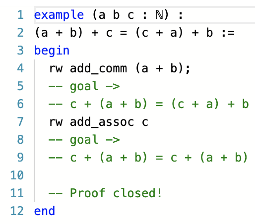
(a) LEAN, rw stands for rewrite

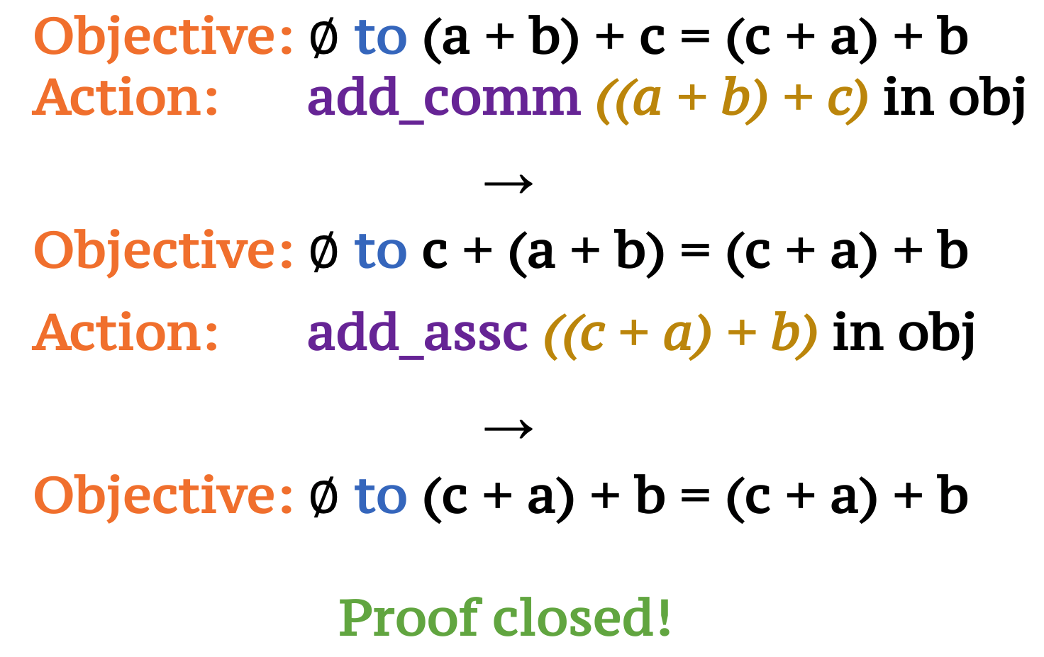
(b) INT, seq2seq interface

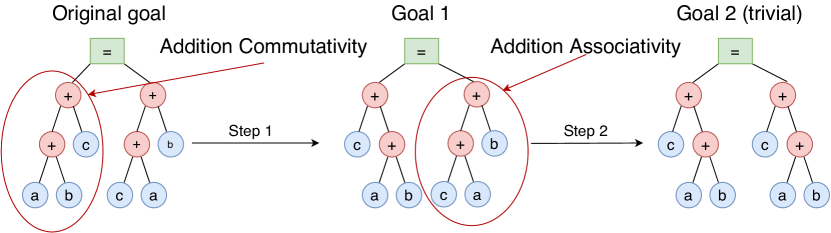
(c) INT, graph interface

Figure 1: A proof of $a+b+c=c+a+b$ in LEAN and INT, with seq2seq and graph interfaces.

We built a lightweight proof assistant to interact with theorem provers. It has two interfaces, providing theorem provers with sequential and graph representations of the proof state, respectively.

A problem in INT is represented by a goal and a set of premises (e.g. $a+0=a,\varnothing$), which are mathematical propositions. The INT assistant maintains a proof state composed of the goal and the proven facts. The proof state is initialized to be just the goal and premises of the theorem. A proof is a sequence of axiom-arguments tuples (e.g. $[(\text{AdditionZero},[a+0])]$). At each step of the proof, a tuple is used to produce a logical relation in the form of assumptions $\to$ conclusions (e.g. $\varnothing\to a+0=a$). Then, if the assumptions are in the proven facts, the conclusions are added to the proven facts; if the conclusions include the goal, the unproven assumptions will become the new goal. The assistant considers the theorem proven, if after all steps in the proof are applied, the goal is empty or trivial.

In Figure 1, we present the same proof in LEAN (de Moura et al., 2015) and INT assistants. They both process proofs by simplifying the goal until it is trivial. The INT assistant’s seq2seq interface (Figure 1(b)) is very similar to that of LEAN (Figure 1(a)) with the rewrite tactic. An action is composed of an axiom followed by argument names and their positions in the proof state. in obj indicates that the arguments can be found in the objective. The graph interface (Figure 1(c)) of the INT assistant allows theorem provers to chose axiom arguments from the computation graphs of the proof state by node. We can view theorem proving with this interface as a graph manipulation task.

INT assistant provides fast simulation. To demonstrate this, we produced 10,000 typical proof steps in both interfaces, 40-character-long on average. We executed them with HOL Light (Harrison, 1996) and INT assistant. The average time it takes per step is 7.96ms in HOL Light and 1.28ms in INT, resulting in a 6.2$\times$ speedup. The correctness of the proofs is ensured by a trusted core of fewer than 200 lines of code.

3.3 Theorem Generator

One of the main contributions of this paper is to provide a generation algorithm that is able to produce a distribution of non-trivial synthetic theorems given an axiom order. Generating theorems by randomly sampling axiom and argument applications will often yield theorems with short proofs. Instead, we write production rules for axioms in the form of transformation and extension rules. With these production rules, we can find arguments and new premises required for longer proofs.

We provide the theorem generation algorithm in Algorithm 1. The general idea of the algorithm is to morph a trivial logic statement into one that requires a non-trivial proof; we call this statement the core logic statement. We initiate the core logic statement $C_{0}$ to be one of the initial conditions. At step $t$ of the generation process, we are given an axiom $a_{t}$ specified by the axiom order. We apply the morph function associated with the axiom $a_{t}$ to $C_{t-1}$ and derive a new logic statement $C_{t}$ and corresponding premises $P_{t}$. The key design idea in the morph function is to ensure that the newly

Algorithm 1 Theorem Generator

1:function generate_theorem(initial conditions $\mathcal{I}$, axiom order $A$)

2:     Axiom order length $L$ = len($A$).

3:     Initialize core logic statement $C_{0}\sim Uniform(\mathcal{I})$, and the set of premises $P=\{C_{0}\}$.

4:     for $t\leftarrow 1$ to $L$ do

5:         Get axiom $a_{t}\leftarrow A[t]$.

6:         Get new logic statement and premises: $C_{t}$, $P_{t}$ $\leftarrow$ morph ($a_{t},C_{t-1}$).

7:         Add new premises to the set of all premises: $P\leftarrow P\cup P_{t}$.

8:     end for

9:     return $C_{L},P$

10:end function

generated logic statement and the premises form the implication $C_{t-1},a_{t},P_{t}\to C_{t}$ (see Appendix B for details). Therefore, we can chain the implications from all steps together to obtain a proof whose length is the axiom order: $C_{0},\{a_{t},P_{t}\}_{t=1}^{L}\to C_{L}$, where $L$ denotes the length. The last core logic statement $C_{L}$ and its premises $C_{0},\{P_{t}\}_{t=1}^{L}$ are returned as the theorem generated. Below we show a step-by-step example of how a theorem is generated with our algorithm.

With recorded axiom and argument applications, we can synthesize proofs to the theorems. The proofs can be used for behavior cloning. Appendix E shows statistics of the generated proofs, including the distribution of length of theorems in characters, the distribution of axioms, and the distribution of the number of nodes in proof state graphs.

4 Experiments

Our experiments are intended to answer the following questions:

1. Can neural agents generalize to theorems: 1) sampled from the same distribution as training data, 2) with different initial conditions, 3) with unseen axiom orders, 4) with unseen axiom combinations, 5) with different numbers of unique axioms, 6) with shorter or longer proofs?

2. How do different architectures (transformer vs. GNN) affect theorem provers’ in-distribution and out-of-distribution generalization?

3. Can search at test time help generalization?

4.1 Experiment Details

In the following experiments, we used the proofs generated by the INT generator to perform behavior cloning. We then evaluated the success rates of trained agents in a theorem proving environment. We denote the cardinality of an axiom combination as $K$ and the length of a proof as $L$. In the worked example, $K=4$ and $L=4$. For each theorem distribution, we first generated a fixed test set of 1000 problems, and then produced training problems in an online fashion, while making sure the training problems were different from the test ones. For each experiment, we generated 1000 problems and performed 10 epochs of training before generating the next 1000. We ran 1500 such iterations in total, with 1.5 million problems generated. We used the Adam optimizer (Kingma and Ba, 2015). We searched over the learning rates $\{10^{-5}$, $3\cdot 10^{-5}$, $10^{-4}$, $3\cdot 10^{-4}\}$ in preliminary experiments and found $10^{-4}$ to be the best choice, which was used for following experiments. We used one Nvidia P100 or Tesla T4 GPU with 4 CPU cores for training. For each experiment, we ran 2 random seeds, and picked the one with higher validation success rates for test evaluation. Since this paper focuses on inequalities, all figures and tables in the main text are based on results from the ordered-field axiomization. We also include results of GNN-based agents on equalities in Appendix G.

4.2 Network Architectures

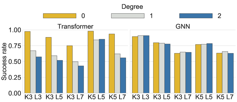
Figure 2: Proof success rates on problems generated with different $K$ and $L$ parameters. Left: When the IID assumption holds, the success rate decreases as the two generation parameters $K$ and $L$ are increased. Right: All agents are trained on degree-0 problems and evaluated against problems of degree 0, 1, and 2. We find that transformer-based agents deteriorate in performance as the test problems become more complex than training problems. For GNN-based agents, there are no obvious trends as to how the proof success rate changes as the degree of the initial entities is varied.

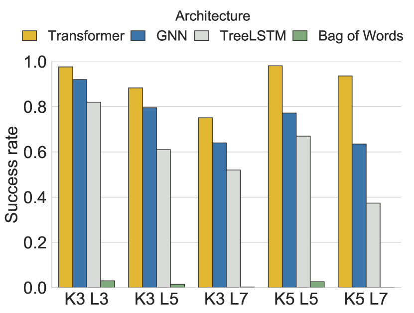
Figure 3: Proof success rates on test problems generated with $K$ and $L$ settings. Transformer and GNN perform well; TreeLSTM has mediocre performance; and Bag-of-Words performs poorly: it cannot prove more than 5% of problems.

In this section, we introduce four baselines built on commonly used architectures: Transformers (Vaswani et al., 2017), Graph Neural Networks (GNNs), TreeLSTMs (Tai et al., 2015) and Bag-of-Words (BoWs). In preliminary experiments, we found Graph Isomorphism Networks (GINs) (Xu et al., 2019) to have performed the best among several representative GNN architectures. So we used GIN as our GNN of choice. Transformers interact with the INT proof assistant through the seq2seq interface while the other baselines through the graph interface.

For sequence-to-sequence training, we used a character-level transformer architecture with 6 encoding layers and 6 decoding layers. We used 512 embedding dimensions, 8 attention heads and 2048 hidden dimensions for position-wise feed-forward layers. We used dropout with rate 0.1, label smoothing with coefficient 0.1, and a maximum 2048 tokens per batch. The library fairseq (Ott et al., 2019) was used for its implementation.

For data in the graph form, each node in computation graphs corresponds to a character in the formula. We first used a learnable word embedding of dimension 512 to represent each node. We then used 6 GIN layers to encode graph inputs into vector representations, each with 512 hidden dimensions. The graph representation was obtained by taking the sum of all the node embeddings. For the TreeLSTM and the BoW baselines, we used a bidirectional TreeLSTM with 512 hidden dimensions and a BoW architecture to compute the graph representation vectors from node embeddings. The hyper-parameters used were found to be optimal in preliminary experiments. We then proposed axioms conditioned on the graph representations, with a two-layer MLP of hidden dimension 256. Conditioning on the graph representation and axiom prediction, the arguments are selected in an autoregressive fashion. Namely, the prediction of the next node is conditioned on the previous ones. For each argument prediction, we used a one-layer MLP with a hidden size of 256. We used graph neural network libraries Pytorch Geometric (Fey and Lenssen, 2019) for the GIN implementation, and DGL (Wang et al., 2019) for the TreeLSTM implementation.

We trained agents based on architectures mentioned above by behavior cloning on theorems of various length ($L$) and number of axioms ($K$). The success rates for proving 1000 test theorems are plotted in Figure 3. As the BoW architecture did not utilize the structure of the state, it failed miserably at proving theorems, indicating the significance of the structural information. TreeLSTM performed worse than the graph neural network baseline. The transformer and the GNN baselines perform the best among the architectures chosen and they take inputs in sequential and graph forms, respectively. Thus, we used these two architectures in the following experiments to investigate generalization.

4.3 Benchmarking Six Dimensions of Generalization

IID Generalization

In this experiment, the training and test data are independently and identically distributed (IID). The performances of our transformer-based and GNN-based agents are displayed on the left in Figure 2. As can be seen, the performance of agents examined on train and test problems are very similar. The largest difference between train and test success rates is $2\%$ ($K3L7$). Notably, transformer-based agents complete $15.3\%$ more test proofs than GNN-based agents on average.

Initial Condition

Consider two theorems: (1) $(a+b)^{2}=a^{2}+b^{2}+2ab$ and (2) $(a+(b+c))^{2}=a^{2}+(b+c)^{2}+2a(b+c)$. The two problems take the same axioms and the same number of steps to prove. However, the axiom argument complexities are different, which can be seen as a result of varying initial conditions. Can agents trained on problems like (1) prove theorems like (2)?

For an initial condition of the form $X=X$, we use the degree of the entity $X$ to determine the complexity. In this experiment, we trained agents on problems with initial conditions made up of entities of degree 0, and evaluated them on ones of degrees 1 and 2. The results are presented in Figure 2 (b) with various $K$ and $L$. For transformer-based agents, the success rate drops $25.6\%$ on degree-1 problems and $31.5\%$ on degree-2 problems on average. However, for GNN-based agents, the largest generalization gap between training and test success rates is $3\%$ ($K3L5$). This shows that GNN agents can generalize to problems of higher complexities while transformer agents struggle.

Axiom Orders

Table 1: Left: Average success rates (in %) of agents trained on different numbers of axiom orders. Right: Average success rates (in %) of agents trained on different numbers of axiom combinations.

# Axiom 100 500 2000 5000 orders Train Test Train Test Train Test Train Test Transformer 93.2 10.0 93.4 62.8 93.6 87.9 93.7 91.8 GNN 87.6 21.1 86.6 53.6 79.0 70.4 75.7 74.7

# Axiom 25 100 200 300 combinations Train Test Train Test Train Test Train Test Transformer 96.1 29.3 96.0 71.8 95.4 88.4 94.4 91.3 GNN 79.1 47.5 76.6 68.0 72.6 72.4 72.8 71.9

Let $A$ and $B$ represent two different axioms. There are multiple orders in which they can be applied in a $K2L3$ problem. $O_{1}$ = [$A$, $A$, $B$] and $O_{2}$ = [$B$, $A$, $B$] are two examples. Can an agent trained on problems generated with $O_{1}$ prove theorems generated with $O_{2}$?

For both architectures, we investigated how well agents can generalize to problems with different axiom orders than those in training. We generated 100, 500, 2000, and 5000 axiom orders to use in the training set for different $K$ and $L$ settings. We evaluated the test success rates on 1000 unseen axiom orders with the corresponding $K$ and $L$ settings and averaged them. The results averaged over different $K$ and $L$ settings are shown on the left of Table 1 (See Appendix G.5 for the full results).

It can be observed in the table that the test success rates rise when we increase the number of axiom orders in the training set. We notice that transformer-based agents have worse generalization than GNN-based ones, as their average generalization gap is larger. This is particularly true when the number of axiom orders in the training set is 100: transformer-based agents can prove only $10.0\%$ of test theorems. Remarkably, they still manage to complete more proofs than GNNs when the number of axiom orders in the training set exceeds 500.

Axiom Combinations

Consider three problems provable in the ordered field axiomization (Appendix A): (1) $a^{2}\geq 0$, (2) $a*(b+c)=b*a+a*c$, and (3) $a^{2}+b^{2}-2ab\geq 0$. Solving (1) requires axiom SquareGEQZero (SGEQZ). Solving (2) requires axiom AdditionMultiplicationDistribution (AMD) and axiom MultiplicationCommutativity (MC). Solving (3) requires axiom SGEQZ and axiom AMD. Notice that all axioms used to prove (3) appear in the proofs of (1) and (2). We ask: can an agent trained on theorems like (1) and (2) prove theorems like (3)?

In this set of experiments, we investigated how well theorem provers can generalize to problems with different axiom combinations than those in training for both architectures. We used 25, 100, 200, and 300 axiom combinations to generate the training set with various $K$ and $L$ settings, and evaluated the agents on test sets generated with 300 unseen combinations. The results averaged over different $K$ and $L$ settings are displayed on the right in Table 1 (See Appendix G.5 for full results). As the number of axiom combinations in training set increases, the generalization gap decreases and test success rate improves. The transformer-based agents have larger generalization gaps than GNN-based ones. This is particularly obvious when there are 25 axiom combinations: the generalization gap is $66.8\%$ for transformers and $31.6\%$ for GNNs. The test success rate of transformers is $18.2\%$ lower than that of GNNs in this setting. Yet when there are more than 100 axiom combinations in training, transformers always perform better on the test sets, completing $3.8\%-19.6\%$ more proofs. When the data is diverse, transformers perform better; when it is insufficient, GNNs are better. This might be due to the difference in the inductive bias used by both structures and might explain the choice of neural architectures in deep learning practice.

Number of Axioms

Here we investigated how well theorem provers could generalize to test problems that were generated with a different number of axioms than at training time. For instance, let $A$, $B$ and $C$ represent different axioms. Will agents trained on $K2L3$ axiom orders like $[A,B,A]$ and $[C,C,B]$ be able to prove theorems generated with $K3L3$ axiom orders like $[A,B,C]$?

We trained the agents on problems that have the same proof length ($L=7$) and varying $K$s. The results are on the left of Figure 4. It can be observed from the figure that in general, agents perform the best on the $K$ they were trained on and worse when $K$ shifts away. Transformer-based agents showed better performances in all $K$ and $L$ settings, completing $20.9\%$ more proofs than GNN-based ones on average. The success rates of transformer-based agents drop $5.6\%$ on average when the test $K$ is shifted away by 1 from the training $K$. For GNN-based agents, this averages to $5.1\%$. This shows that their generalization abilities to different number of axioms are similar.

Proof Length

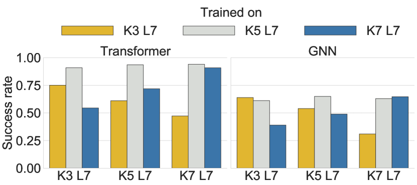
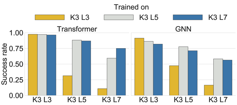
Figure 4: Proof success rates on problems generated with different parameters. Left: We keep $L$ the same and vary $K$. The success rate is likely to decrease when the test problems have different $K$ from the training problems. Right: We keep $K$ the same and vary $L$. For all agents, the proof success rate is lower on theorems that require longer proofs.

We tested the generalization ability of theorem provers over the dimension of proof length of the theorems. To do this, we kept the cardinality of the axiom set to be the same ($K=3$) and varied the evaluated problems’ proof length ($L=3,5,7$). The result is presented on the right of Figure 4. For all of the agents trained, the success rate decreases as the length of the proof increases. This is due to the natural difficulty of completing longer proofs. Observing the figure, we see that the longer the training problems, the less they deteriorate in performance when proofs becomes longer: agents trained on $K3L3$ problems complete $18.8\%$ fewer proofs when $L$ is increased by 1, while ones trained on $K3L7$ complete $5.7\%$ fewer. Furthermore, the performance of transformer-based agents decreases by $12.2\%$ when the test proof length increases by 1, compared to $10.7\%$ for GNN-based ones. This suggests that transformers have inferior proof length generalization abilities than GNNs.

4.4 Generalizing with Search

We investigated whether performing search at test time can help agents generalize. Specifically, we investigated the effectiveness of Monte-Carlo Tree Search (MCTS) in finding proofs for unseen theorems with GNN-based agents. We chose GNN-based agents because they are better at out-of-distribution generalization than transformer-based ones. Straightforward application of MCTS is impractical: in our theorem proving environment, the action space can be as large as 1.3M in size (see Appendix H). Hence, it would be infeasible to expand all possible actions when constructing the MCTS trees. Thus, we only performed MCTS over the axiom space ($18$ distinct axioms in total), and the arguments were proposed by the behavior cloning agents. Following AlphaGo Zero/AlphaZero (Silver et al., 2017; 2018), we trained a value network to estimate the value of a state. The value network is an MLP with two hidden layers of size 256, taking the GNN global representations of graphs as input. It was trained on 1000 episodes of rollouts obtained by the behavior cloning agents, with a learning rate of $3\cdot 10^{-6}$. We also followed AlphaZero for the choice of the upper confidence bound, and the way that actions are proposed using visit counts. We used 200 simulations for constructing MCTS trees. More details can be found in Appendix F. We took the agents trained on "$K3L3$", "$K3L5$", and "$K3L7$" from section 4.3, and evaluated the agents’ performance when boosted by MCTS.

Table 2: The behavior cloning (BC) agents versus the MCTS-assisted (search) agents. Left: The average success rates (in %) of agents with and without MCTS over 1000 test theorems. Right: The average length of successful proofs by agents with and without MCTS over 1000 test theorems. $K$ denotes the cardinality of the axiom combination of a proof, $L$ denotes the length of the proof.

Train K3L3 K3L5 K3L7 Evaluation BC Search BC Search BC Search K3 L3 92 98 91 97 81 96 K3 L5 50 64 80 92 70 92 K3 L7 25 40 64 78 58 81 Average 56 67 78 89 69 90

Train K3L3 K3L5 K3L7 Evaluation BC Search BC Search BC Search K3 L3 3.83 3.33 4.00 3.52 5.00 3.67 K3 L5 7.54 6.82 6.2 5.52 6.84 5.56 K3 L7 9.05 8.54 8.01 7.53 8.39 7.50 Average 6.81 6.23 6.07 5.52 6.74 5.58

Generalization

The average success rates on 1000 test theorems are presented on the left in Table 2. We can see that search greatly improved the generalization results. It helped to solve $21\%$ more problems on average for the agent trained on theorem distribution $K3L7$. Remarkably, when evaluating on $K3L7$ theorems, search helped the $K3L3$ agent improve its success rate from $25\%$ to $40\%$: a relative improvement of $60\%$. It is interesting to see the $K3L7$ behavior cloning agent solved $9\%$ fewer problems on average than the $K3L5$ agent. But search brought about much larger improvement to the $K3L7$ agent and helped it to solve the largest proportion of problems on average – $90\%$. This indicates that skills learned through behavior cloning can be better exploited by searching.

The average proof length for 1000 problems is presented on the right in Table 2 (we count those unsolved problem as 15, the step limit of an episode). We can see that by performing search, we are able to discover proofs of length closer to the ground truth proof length. For test theorems requiring 3-step proofs, the $K3L3$ agent was able to prove them in 3.33 steps on average, with a gap of 0.33 steps to the optimal value. Similarly, for test theorems requiring 5-step proofs, the $K3L5$ agent was able to prove them in 5.52 steps on average, with a gap of 0.52 steps; and for theorems requiring 7-step proofs, $K3L7$ agent achieved a gap of 0.5 steps.

4.5 Discussion

Experimental results suggested that transformer-based agents can complete more proofs in the IID generalization scenario but have larger out-of-distribution generalization gaps than GNN-based ones. The larger gap may be due to the lack of constraints in the sequence-to-sequence framework, in which the model can propose sequences that are invalid actions, whereas the graph interface constrains the model to propose valid actions only. However, we still see that transformers are able to complete more proofs overall. This shows the superiority of transformers in model capacity when applied to theorem proving. This insight motivates us to explore the possibility of taking the best from both worlds, combining both graph structural information and the strong transformer architecture to improve learning-assisted theorem proving. We leave it for future work.

5 Conclusion

We addressed the problem of diagnosing the generalization weaknesses in learning-assisted theorem provers. We constructed INT, a synthetic benchmark of inequalities, to analyze the generalization of machine learning methods. We evaluated transformer-based and GNN-based agents and a variation of GNN-based agents with MCTS at test time. Experiments revealed that transformer-based agents generalize better when the IID assumption holds while GNN-based agents generalize better in out-of-distribution scenarios. We also showed that search can boost the generalization ability of agents. We stress that proving theorems in INT is not an end in itself. A hard-coded expert system might perform well on INT but not generalize to real-world mathematical theorems. Therefore, INT should be treated as instrumental when diagnosing generalization of agents. The best practice is to use INT in conjunction with real mathematical datasets.

We believe our benchmark can also be of interest to the learning community, facilitating research in studying generalization beyond the IID assumption. The agents’ abilities to reason and to go beyond the IID assumption are essential in theorem proving, and studying how to acquire these abilities is at the frontier of learning research. In other domains requiring out-of-distribution generalization, such as making novel dialogs (Chen et al., 2017) or confronting unseen opponents in Starcraft (Vinyals et al., 2019), the requirements for data and computation forbid a generally affordable research environment. The INT benchmark provides practical means of studying out-of-distribution generalization.

Appendix

Appendix Appendix A Axiom Specifications

Table 3:

Field axioms	Definition
(rl) AdditionCommutativity (AC)	$\to a+b=b+a$
(rl) AdditionAssociativity (AA)	$\to a+(b+c)=(a+b)+c$
(rl) AdditionSimplification (AS)	$a=b\to a+(-b)=0$
(rl) MultiplicatoinCommutativity (MC)	$\to a\cdot b=b\cdot a$
(rl) MultiplicationAssociativity (MA)	$\to a\cdot(b\cdot c)=(a\cdot b)\cdot c$
(rl) MultiplicationSimplification (MS)	$(a\neq 0)\land(a=b)\to 1=a\cdot\frac{1}{b}$
(rl) AdditionMultiplicationLeftDistribution (AMLD)	$\to(a+b)\cdot c=a\cdot c+b\cdot c$
(rl) AdditionMultiplicationRightDistribution (AMRD)	$\to a\cdot(b+c)=a\cdot b+a\cdot c$
(rl) SquareDefinition (SD)	$\to a^{2}=a\cdot a$
(rl) MultiplicationOne (MO)	$\to a\cdot 1=a$
(rl) AdditionZero (AZ)	$\to a+0=a$
(rl) PrincipleOfEquality (POE)	$(a=b)\land(c=d)\to a+c=b+d$
(rl) EquMoveTerm(Helper axiom) (EMT)	$a+b=c\to a=c+(-b)$
Ordered field axioms	Definition
(rl) All field axioms
(rl) SquareGEQZero (SGEQZ)	$a=b\to a\cdot b\geq 0$
(rl) EquivalenceImpliesDoubleInequality (EIDI)	$a=b\to(a\geq b)\land(a\leq b)$
(rl) IneqMoveTerm (IMT)	$a+b\geq c\to a\geq c+(-b)$
(rl) FirstPrincipleOfInequality (FPOI)	$(a\geq b)\land(c\geq d)\to a+c\geq b+d$
(rl) SecondPrincipleOfInequality (SPOI)	$(a\geq b)\land(c\geq 0)\to a\cdot c\geq b\cdot c$

Appendix Appendix B The morph Function

We detail the morphing of $C$ at each step as follows. For each theorem $a$, we define two symbolic patterns: $\mathcal{L}_{a}$ and $\mathcal{R}_{a}$, each represented by an expression (see Appendix C for full details). For example, if $a$ is AdditionCommutativity, we use $\mathcal{L}_{a}=x_{1}+x_{2}$ to denote any formula that is a sum of two terms ($x_{1}$ and $x_{2}$ can be arbitrary terms). We check if one of the nodes in the computation graph of $C$ has the structure defined by $\mathcal{L}_{a}$. If so, we then transform that node to a formula specified by $\mathcal{R}_{a}$. For example, if $C$ is $(p+q)+l=(p+(q+l))$, $p+q$ is a node that matches the pattern specified by $\mathcal{L}_{a}$, in which $x_{1}=p$ and $x_{2}=q$. Let $\mathcal{R}_{a}=x_{2}+x_{1}$. We hence transform the node $p+q$ to $q+p$ as specified by $\mathcal{R}_{a}$. As a result, $C^{\prime}$ becomes $(q+p)+l=(p+(q+l))$. If there is no node in the computation graph, we morph the core logic statement using the extension function $\mathcal{E}$, defined in Appendix D . We sample nodes in available computation graphs and combine them with $C$, coming up with $C^{\prime}$ and optionally a non-empty set of new premises $P_{new}$.

Algorithm 2 Theorem Generator (complete)

1:function generate_theorem(initial conditions $\mathcal{I}$, axiom order $A$)

2:     Axiom order length $L$ = len($A$).

3:     Initialize core logic statement $C_{0}\sim Uniform(\mathcal{I})$, and the set of premises $P=\{C_{0}\}$.

4:     for $t\leftarrow 1$ to $L$ do

5:         Get axiom $a_{t}\leftarrow A[t]$.

6:         Get new logic statement and premises: $C_{t}$, $P_{t}$ $\leftarrow$ morph ($a_{t},C_{t-1}$).

7:         Add new premises to the set of all premises: $P\leftarrow P\cup P_{t}$.

8:     end for

9:     return $C_{L},P$

10:end function

function morph(axiom $a$, core logic statement $C$)

2:     Collect $\mathcal{N}_{t}=\{n|\text{ n is a node in}\ C\ \text{and matches the pattern specified by }\mathcal{L}_{a}\}$

     if $\mathcal{N}_{t}\neq\varnothing$ then

4:         Sample node $n\sim Uniform(\mathcal{N}_{t})$.

         Transform $n$ into new node $n^{\prime}$ using the mapping from $\mathcal{L}_{a}$ to $\mathcal{R}_{a}$.

6:         $C^{\prime}\leftarrow$ Replace $n$ with $n^{\prime}$ in the graph of $C$. $P_{new}\leftarrow\varnothing$.

     else

8:         Collect $\mathcal{N}$, the set of all nodes in the graphs.

         Extend $C$ and get the set of premises: $C^{\prime},P_{new}\leftarrow\mathcal{E}(a,C,\mathcal{N})$.

10:     end if

     return $C^{\prime},P_{new}$.

12:end function

The reasons that we have two sets of rules for morphing are as follow: 1) Transformation rules can only be applied when the axiom will produce an equality, while extension rules can be applied to any axiom. So in order to generate theorems with all the axioms, we need the extension rules. 2) Almost all the extension rules will complicate the core logic statement while none of the transformation rules will. If we only have extension rules, the goal generated can be very complex even the proof is of moderate length. In order to generate compact theorems (goal not too complicated) with long proofs, the transformation rules are preferred. Therefore we only apply extension rules when transformation rules are not applicable.

Appendix Appendix C Transformation Rules

The implementations of the transformation rules $\mathcal{L}$ and $\mathcal{R}$.

Table 4:

Axiom ($a$)	$\mathcal{L}_{a}$	$\mathcal{R}_{a}$
AdditionCommutativity	$x_{1}+x_{2}$	$x_{2}+x_{1}$
AdditionAssociativity	$x_{1}+(x_{2}+x_{3})$	$(x_{1}+x_{2})+x_{3}$
AdditionSimplification	$x_{1}+(-x_{1})$	$0$
MultiplicatoinCommutativity	$x_{1}\cdot x_{2}$	$x_{2}\cdot x_{1}$
MultiplicationAssociativity	$x_{1}\cdot(x_{2}\cdot x_{3})$	$(x_{1}\cdot x_{2})\cdot x_{3}$
MultiplicationSimplification	$x_{1}\cdot\frac{1}{x_{1}}$	$1$
AdditionMultiplicationLeftDistribution	$(x_{1}+x_{2})\cdot x_{3}$	$x_{1}\cdot x_{3}+x_{2}\cdot x_{3}$
AdditionMultiplicationRightDistribution	$x_{1}\cdot(x_{2}+x_{3})$	$x_{1}\cdot x_{2}+x_{1}\cdot x_{3}$
SquareDefinition	$x_{1}^{2}$	$x_{1}\cdot x_{1}$
MultiplicationOne	$x_{1}\cdot 1$ or $1\cdot x_{1}$	$x_{1}$
AdditionZero	$x_{1}+0$ or $0+x_{1}$	$x_{1}$
SquareGEQZero	NA	NA
PrincipleOfEquality	NA	NA
EquMoveTerm	NA	NA
EquivalenceImpliesDoubleInequality	NA	NA
IneqMoveTerm	NA	NA
FirstPrincipleOfInequality	NA	NA
SecondPrincipleOfInequality	NA	NA

Appendix Appendix D Extension Function

For these axioms, the core logic statement $C$ needs to be of the form LHS($C$) = RHS($C$).

Table 5:

Axiom ($a$)	Extension function $\mathcal{E}(C,a,\mathcal{N})$
AdditionCommutativity	Sample node $n\sim$ Uniform ( $\mathcal{N}$)
	return RHS($C$) $+n=n+$ LHS($C$), $\varnothing$
AdditionAssociativity	Sample nodes $n_{1},n_{2}\sim$ Uniform ( $\mathcal{N}$)
	return RHS($C$)$+(n_{1}+n_{2})=$LHS($C$)$+n_{1}+n_{2}$, $\varnothing$
AdditionSimplification	return $0=$LHS($C$)$+(-$RHS($C$)$)$, $\varnothing$
MultiplicatoinCommutativity	Sample node $n\sim$ Uniform ( $\mathcal{N}$)
	return RHS($C$)$\cdot n=n\cdot$LHS($C$), $\varnothing$
MultiplicationAssociativity	Sample nodes $n_{1},n_{2}\sim$ Uniform ( $\mathcal{N}$)
	return RHS($C$)$\cdot(n_{1}\cdot n_{2})=$LHS($C$)$\cdot n_{1}\cdot n_{2}$, $\varnothing$
MultiplicationSimplification	return $1=$LHS($C$)$\cdot$ $\frac{1}{\text{RHS}(C)}$, $\varnothing$
AdditionMultiplicationLeftDistribution	Sample nodes $n_{1},n_{2}\sim$ Uniform ( $\mathcal{N}$)
	return $(n_{1}+n_{2})\cdot\text{RHS}(C)=$
	$n_{1}\cdot\text{LHS}(C)+n_{2}\cdot\text{LHS}(C),\varnothing$
AdditionMultiplicationRightDistribution	Sample nodes $n_{1},n_{2}\sim$ Uniform ($\mathcal{N}$)
	return $\text{RHS}(C)\cdot(n_{1}+n_{2})=$
	$\text{LHS}(C)\cdot n_{1}+\text{LHS}(C)\cdot n_{2},\varnothing$
SquareDefinition	return $\text{LHS}(C)\cdot\text{RHS}(C)=\text{LHS}(C)^{2}$, $\varnothing$
MultiplicationOne	return Uniform ( {$\text{LHS}(C)\cdot 1=\text{RHS}(C)$,
	$1\cdot\text{LHS}(C)=\text{RHS}(C)$ } ), $\varnothing$
AdditionZero	return Uniform ( {$\text{LHS}(C)+0=\text{RHS}(C)$,
	$0+\text{LHS}(C)=\text{RHS}(C)$ } ), $\varnothing$
SquareGEQZero	return LHS($C$) $\cdot$ RHS($C$) $\geq 0$, $\varnothing$
PrincipleOfEquality	Sample nodes $n_{1},n_{2}\sim\mathcal{N}$, where $n_{1}=n_{2}$
	return LHS($C$) + $n_{1}$ = RHS($C$) + $n_{2}$, {$n_{1}=n_{2}$}
EquMoveTerm	Only execute when LHS($C$) is of the form $x+y$
	return $x=\text{RHS}(C)+(-y)$, $\varnothing$
EquivalenceImpliesDoubleInequality	return LHS($C$) $\geq$ RHS($C$), $\varnothing$

For these axioms, the core logic statement $C$ needs to be of the form LHS($C$) $\geq$ RHS($C$).

Table 6:

Axiom ($a$)	Extension function $\mathcal{E}(C,a,\mathcal{N})$
IneqMoveTerm	Only execute when LHS($C$) is of the form $x+y$
	return $x\geq\text{RHS}(C)+(-y)$, $\varnothing$
FirstPrincipleOfInequality	Sample nodes $n_{1},n_{2}\sim\mathcal{N}$, where $n_{1}\geq n_{2}$
	return LHS($C$) + $n_{1}$ $\geq$ RHS($C$) + $n_{2}$, {$n_{1}\geq n_{2}$}
SecondPrincipleOfInequality	Sample node $n\sim\mathcal{N}$, where $n\geq 0$
	return LHS($C$) $\cdot n\geq$ RHS($C$) $\cdot n$, {$n\geq 0$}

Appendix Appendix E Dataset Statistics

Appendix E.1 Theorem Length

We compare the length of the theorems generated in characters and plot their distributions in Figure 5. The length of the theorem in characters is a measure for how complicated it is. As is expected, the more complicated the theorem is, the longer the proof(bigger $L$). It is also worth noting that as $L$ becomes bigger, the distribution of theorem length becomes less concentrated. This is likely a consequence of a more spread-out theorem length range.

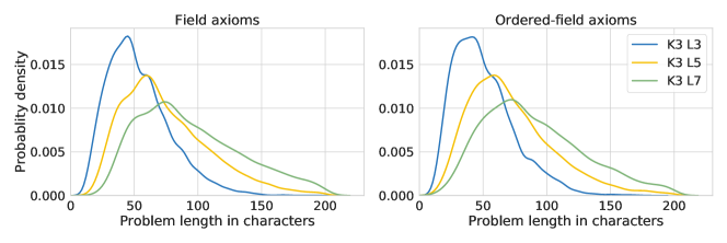
Figure 5: The distribution of theorem length in characters for field axioms(left) and ordered-field axioms(right) generated with parameters $K3L3$, $K3L5$, and $K3L7$. As the length of the proof is increased, so is the number of characters in the theorem, while the distribution of latter is less concentrated.

Appendix E.2 Axiom Distributions

The frequency at which each axiom is applied influences the distribution of theorems our generator is able to produce. In Figure 6, we present the proportions of axioms that are applied in generating 10,000 theorems. Their frequencies are a measure of how easy it is to satisfy the conditions to apply them. For the field axioms, the PrincipleOfEquality axiom is the most frequently used(9.30%) and the EquMoveTerm axiom is the most rarely used(2.38%). EquMoveTerm has a strict condition for application: the left hand side of the core logic statement has to be of the form $x+y$, therefore not frequently applied. For the ordered-field axioms, the EquivalenceImpliesDoubleInequality axiom is the most frequently used(10.18%). Since we start with a trivial equality in generation and want to end up with an inequality, a transition from equality to inequality is needed. Among the ways of transitioning, this conditions to apply this axiom is easiest to satisfy. Its popularity is followed by the group of Field axioms, from MultiplicationCommutativity(4.69%) to AdditionAssociativity(5.98%). The rest are ordered-field axioms which define the properties of inequalities, proportions ranging from IneqMoveTerm(1.14%) to FirstPrincipleOfInequality(5.74%).

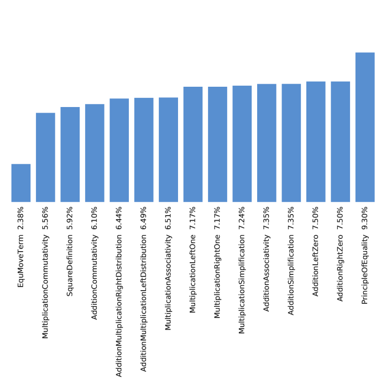
(a) Field axiom distribution

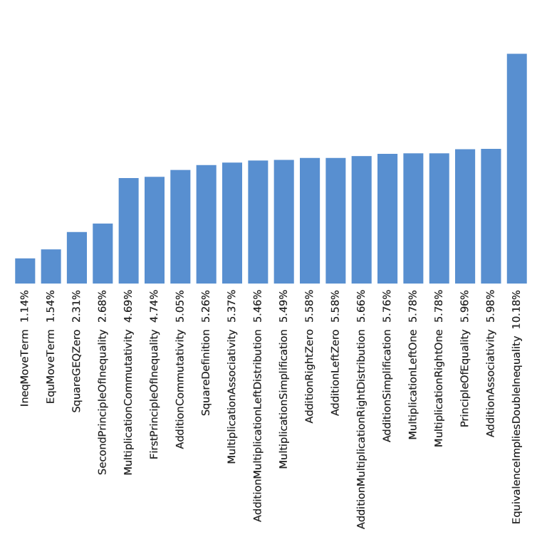
(b) Ordered-field axiom distribution

Figure 6:

Appendix E.3 Number of Nodes

Since an action in the MDP consists of an axiom and a list of nodes as its arguments and the number of axioms is fixed, the number of nodes available determines the size the action space. Therefore it is interesting to investigate how many nodes are available in a proof. In Figure 7 we present the average number of nodes in proofs of different length. It can be told from the figure that the longer the proofs, the more nodes there will be, as expected. Comparing the axiom sets used, we find that the average number of nodes for ordered-field axioms is larger than that of field axioms. This is likely the consequence of ordered-field axioms, in generation, being more capable of producing new premises(e.g. First Principle of Inequality will produce an inequality premise(see Table LABEL:table:_inequality_generation_axioms), thus adding more nodes in the graphs).

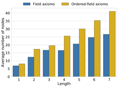
Figure 7:

Appendix Appendix F More Experimental Details for Generalization with Search

We give more experimental details for the use of MCTS. Following [Silver et al., 2017], in the selection step of the MCTS tree construction, we use the following formula to select the next action,

$$a^{*}=\mathrm{argmax}_{a}\left(Q(s,a)+c_{\mathrm{puct}}P(s,a)\frac{\sqrt{\sum_{b}N(s,b)}}{1+N(s,a)}\right),$$

where $Q(s,a)$ represents the action value function, $N(s,a)$ denotes the visit counts, $P(s,a)$ is the prior probability, and $c_{\mathrm{puct}}$ is a constant hyperparameter. In all of our experiments, we used the behavior cloning policy for computing $P(s,a)$, and we used $c_{\mathrm{puct}}=1$. After the MCTS tree is built, the action is sampled from the policy distribution $\pi(a|s)=N(s,a)^{\frac{1}{\tau}}$, where $\tau$ is a hyperparameter and was chosen as 1 in our experiments.

Appendix Appendix G More Training and Evaluation Results

Appendix G.1 learning curves of GNN-based agents

Figure 8: Proof success rates for field axioms(left) and ordered-field axioms(right) of GNN-based agents trained on different $K$ and $L$ parameters. We keep the $K$ the same and vary the $L$. The agents converge slower and to a lower success rate when the proof length is increased. Also, the agents on field axioms are easier to train than those on ordered-field axioms.

Appendix G.2 Performance variation of trained agents

To verify that the experimental results are statistically significant, we ran the experiments on proof length generalization in subsection 4.3 with 5 random seeds and tabled the results.

Table 7: Success rates of agents trained and tested on problems of different parameters (mean $\pm$ std) in percentage.

Transformers	Tested on	K3 L3	K3 L5	K3 L7
Trained on	K3 L3	97.6 $\pm$ 0.9	31.5 $\pm$ 1.6	10.9 $\pm$ 1.0
	K3 L5	97.2 $\pm$ 0.7	88.3 $\pm$ 1.2	59.5 $\pm$ 1.6
	K3 L7	96.6 $\pm$ 1.2	87.0 $\pm$ 1.6	75.1 $\pm$ 1.2
GNNs	Tested on	K3 L3	K3 L5	K3 L7
Trained on	K3 L3	91.5 $\pm$ 0.5	45.6 $\pm$ 1.7	16.5 $\pm$ 0.8
	K3 L5	86.4 $\pm$ 0.9	77.8 $\pm$ 0.9	58.4 $\pm$ 1.5
	K3 L7	82.0 $\pm$ 1.3	71.4 $\pm$ 1.1	56.5 $\pm$ 1.5

Appendix G.3 GNN-based agents on IID Generalization

Figure 9: Proof success rates on problems generated with different $K$ and $L$ parameters ($K$ denotes the cardinality of the axiom combination of a proof, $L$ denotes the length of the proof). When the IID assumption holds, the success rate decreases as the two generation parameters $K$ and $L$ are increased.

Appendix G.4 GNN-based agents on initial condition generalization

Figure 10: Proof success rates on problems generated with different $K$ and $L$ parameters ($K$ denotes the cardinality of the axiom combination of a proof, $L$ denotes the length of the proof). When generalizing to different initial conditions, there are no obvious trends as to how the proof success rate changes as the degree of the initial entities is varied.

Appendix G.5 Full Results on Axiom Orders and Combinations Generalization

Table 8: Top: Proof success rates (in %) of agents trained on different numbers of axiom orders. Bottom: Proof success rates (in %) of agents trained on different numbers of axiom combinations. $K$ denotes the cardinality of the axiom combination of a proof, $L$ denotes the length of the proof.

Architecture Axiom 100 500 2000 5000 orders Train Test Train Test Train Test Train Test Transformer K3 L3 98.4 32.6 99.5 90.0 98.8 98.7 97.6 97.6 K3 L5 95.3 6.3 94.0 56.3 94.0 94.9 96.5 94.9 K3 L7 87.8 3.8 88.0 46.4 88.3 77.5 88.4 85.5 K5 L5 94.7 5.6 97.0 72.9 97.4 93.1 97.5 96.9 K5 L7 89.7 1.8 88.6 48.6 89.3 75.2 88.6 84.0 Average 93.2 10.0 93.4 62.8 93.6 87.9 93.7 91.8 GNN K3 L3 84.3 38.6 94.4 73.9 93.7 89.0 90.5 92.3 K3 L5 92.7 17.1 86.3 60.0 84.4 72.9 77.7 77.1 K3 L7 82.4 14.1 82.4 33.8 68.6 57.7 70.2 63.5 K5 L5 91.0 23.0 89.7 61.2 81.8 75.0 78.3 80.8 K5 L7 87.5 12.9 80.2 39.0 66.5 57.4 61.6 60.0 Average 87.6 21.1 86.6 53.6 79.0 70.4 75.7 74.7

Architecture Axiom 25 100 200 300 combos Train Test Train Test Train Test Train Test Transformer K3 L3 99.2 34.1 99.0 72.8 99.5 96.1 98.6 98.2 K3 L5 97.8 29.3 98.6 66.3 97.5 89.5 94.3 90.4 K3 L7 93.6 25.0 91.9 55.9 91.5 80.0 91.9 85.9 K5 L5 98.5 27.4 98.4 87.6 97.0 93.6 97.3 94.9 K5 L7 91.2 30.5 92.2 76.3 91.7 82.9 90.0 87.0 Average 96.1 29.3 96.0 71.8 95.4 88.4 94.4 91.3 GNN K3 L3 96.3 61.6 96.0 90.1 92.7 91.2 95.3 92.0 K3 L5 82.1 43.4 80.3 68.9 78.5 74.9 76.5 76.1 K3 L7 72.1 34.3 68.1 57.2 62.3 63.7 62.5 62.0 K5 L5 77.8 61.6 78.9 71.0 74.5 78.4 72.8 74.9 K5 L7 67.2 36.8 59.7 52.7 54.9 54.0 56.7 54.5 Average 79.1 47.5 76.6 68.0 72.6 72.4 72.8 71.9

Appendix G.6 GNN-based agents on axiom number generalization

Figure 11: Proof success rates on problems generated with different parameters (($K$ denotes the cardinality of the axiom combination of a proof, $L$ denotes the length of the proof). We keep parameter $L$ the same and vary parameter $K$. The success rate is likely to decrease when an agent is evaluated on problems that have different $K$ than the problems it is trained on.

Appendix G.7 GNN-based agents on Proof Length Generalization

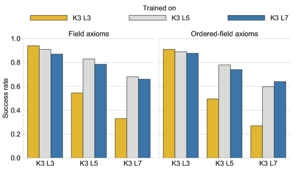
Figure 12: Proof success rates on problems generated with different parameters (($K$ denotes the cardinality of the axiom combination of a proof, $L$ denotes the length of the proof). We keep parameter $K$ the same and vary parameter $L$. For all agents, the proof success rate is lower on theorems that require longer proofs. The best-performing agent for problems of a given length is usually the agent trained on problems of the same length.

Appendix Appendix H Theorem Proving as a Markov Decision Process (MDP)

We model theorem proving as a Markov Decision Process. A state $s$ in the MDP is the proof state maintained by the assistant, namely, the goal, the premises and the proven facts, represented by computation graphs. An action $a$ is a tuple of an axiom and a sequence of arguments. We denote the axiom space as $\mathcal{X}$ and the argument space, the set of all the nodes in available computation graphs, as $\mathcal{N}$. The maximum number of arguments for one axiom within our axiomizations is 3, therefore the action space is $\mathcal{A}=\mathcal{X}\times\mathcal{N}^{3}$. The assistant ignores redundant arguments if fewer than 3 are needed for the axiom considered. We show in Appendix E.3 the distribution of the number of nodes for proofs of different length. The size of the discrete action space can be as large as $18\times 42^{3}\approx 1.33\times 10^{6}$. The deterministic state transition function $P(s,a)$ is implicitly determined by the proof assistant. When the proof assistant deems the proof complete and the theorem proven, the episode terminates and a reward of one is given. Otherwise, the reward is zero at each step. When the step limit for a proof is exhausted, the episode terminates with a reward of zero. For experiments in this paper, we used a step limit of 15.

Appendix Appendix I Example problems

References

- Bansal et al. [2019] Kshitij Bansal, Sarah M. Loos, Markus N. Rabe, Christian Szegedy, and Stewart Wilcox. Holist: An environment for machine learning of higher order logic theorem proving. In Kamalika Chaudhuri and Ruslan Salakhutdinov, editors, Proceedings of the 36th International Conference on Machine Learning, ICML 2019, 9-15 June 2019, Long Beach, California, USA, volume 97 of Proceedings of Machine Learning Research, pages 454–463. PMLR, 2019. URL http://proceedings.mlr.press/v97/bansal19a.html.
- Barras et al. [1999] Bruno Barras, Samuel Boutin, Cristina Cornes, Judicaël Courant, Yann Coscoy, David Delahaye, Daniel de Rauglaudre, Jean-Christophe Filliâtre, Eduardo Giménez, Hugo Herbelin, et al. The Coq proof assistant reference manual. INRIA, version, 6(11), 1999.
- Bridge et al. [2014] James P. Bridge, Sean B. Holden, and Lawrence C. Paulson. Machine learning for first-order theorem proving. Journal of automated reasoning, 53(2):141–172, 2014.
- Chen et al. [2017] Hongshen Chen, Xiaorui Liu, Dawei Yin, and Jiliang Tang. A survey on dialogue systems: Recent advances and new frontiers. Acm Sigkdd Explorations Newsletter, 19(2):25–35, 2017.
- Chvalovskỳ et al. [2019] Karel Chvalovskỳ, Thibault Gauthier, and Josef Urban. First experiments with data driven conjecturing. AITP 2019, 2019. URL http://aitp-conference.org/2019/abstract/AITP_2019_paper_27.pdf.
- Colton [2012] Simon Colton. Automated theory formation in pure mathematics. Springer Science & Business Media, 2012.
- Darvas et al. [2005] Ádám Darvas, Reiner Hähnle, and David Sands. A theorem proving approach to analysis of secure information flow. In International Conference on Security in Pervasive Computing, pages 193–209. Springer, 2005.
- de Moura et al. [2015] Leonardo de Moura, Soonho Kong, Jeremy Avigad, Floris Van Doorn, and Jakob von Raumer. The Lean theorem prover (system description). In International Conference on Automated Deduction, pages 378–388. Springer, 2015.
- Deng et al. [2009] Jia Deng, Wei Dong, Richard Socher, Li-Jia Li, Kai Li, and Fei-Fei Li. Imagenet: A large-scale hierarchical image database. In 2009 IEEE Computer Society Conference on Computer Vision and Pattern Recognition (CVPR 2009), 20-25 June 2009, Miami, Florida, USA, pages 248–255. IEEE Computer Society, 2009. doi: 10.1109/CVPR.2009.5206848. URL https://doi.org/10.1109/CVPR.2009.5206848.
- Dummit and Foote [2004] David Steven Dummit and Richard M Foote. Abstract algebra, volume 3. Wiley Hoboken, 2004.
- Fajtlowicz [1988] Siemion Fajtlowicz. On conjectures of graffiti. In Annals of Discrete Mathematics, volume 38, pages 113–118. Elsevier, 1988.
- Fey and Lenssen [2019] Matthias Fey and Jan Eric Lenssen. Fast graph representation learning with pytorch geometric. CoRR, abs/1903.02428, 2019. URL http://arxiv.org/abs/1903.02428.
- Gauthier [2019] Thibault Gauthier. Deep reinforcement learning in HOL4. CoRR, abs/1910.11797, 2019. URL http://arxiv.org/abs/1910.11797.
- Gauthier [2020] Thibault Gauthier. Deep reinforcement learning for synthesizing functions in higher-order logic. In Elvira Albert and Laura Kovács, editors, LPAR 2020: 23rd International Conference on Logic for Programming, Artificial Intelligence and Reasoning, Alicante, Spain, May 22-27, 2020, volume 73 of EPiC Series in Computing, pages 230–248. EasyChair, 2020. URL https://easychair.org/publications/paper/Tctp.
- Gauthier and Kaliszyk [2015] Thibault Gauthier and Cezary Kaliszyk. Sharing HOL4 and HOL light proof knowledge. In Martin Davis, Ansgar Fehnker, Annabelle McIver, and Andrei Voronkov, editors, Logic for Programming, Artificial Intelligence, and Reasoning - 20th International Conference, LPAR-20 2015, Suva, Fiji, November 24-28, 2015, Proceedings, volume 9450 of Lecture Notes in Computer Science, pages 372–386. Springer, 2015. doi: 10.1007/978-3-662-48899-7\_26. URL https://doi.org/10.1007/978-3-662-48899-7_26.
- Gauthier et al. [2016] Thibault Gauthier, Cezary Kaliszyk, and Josef Urban. Initial experiments with statistical conjecturing over large formal corpora. In Andrea Kohlhase, Paul Libbrecht, Bruce R. Miller, Adam Naumowicz, Walther Neuper, Pedro Quaresma, Frank Wm. Tompa, and Martin Suda, editors, Joint Proceedings of the FM4M, MathUI, and ThEdu Workshops, Doctoral Program, and Work in Progress at the Conference on Intelligent Computer Mathematics 2016 co-located with the 9th Conference on Intelligent Computer Mathematics (CICM 2016), Bialystok, Poland, July 25-29, 2016, volume 1785 of CEUR Workshop Proceedings, pages 219–228. CEUR-WS.org, 2016. URL http://ceur-ws.org/Vol-1785/W23.pdf.
- Gauthier et al. [2017] Thibault Gauthier, Cezary Kaliszyk, and Josef Urban. Tactictoe: Learning to reason with HOL4 tactics. In Thomas Eiter and David Sands, editors, LPAR-21, 21st International Conference on Logic for Programming, Artificial Intelligence and Reasoning, Maun, Botswana, May 7-12, 2017, volume 46 of EPiC Series in Computing, pages 125–143. EasyChair, 2017. URL https://easychair.org/publications/paper/WsM.
- Gauthier et al. [2018] Thibault Gauthier, Cezary Kaliszyk, Josef Urban, Ramana Kumar, and Michael Norrish. Learning to prove with tactics. CoRR, abs/1804.00596, 2018. URL http://arxiv.org/abs/1804.00596.
- Gonthier et al. [2013] Georges Gonthier, Andrea Asperti, Jeremy Avigad, Yves Bertot, Cyril Cohen, François Garillot, Stéphane Le Roux, Assia Mahboubi, Russell O’Connor, Sidi Ould Biha, et al. A machine-checked proof of the odd order theorem. In International Conference on Interactive Theorem Proving, pages 163–179. Springer, 2013.
- Hales et al. [2017] Thomas Hales, Mark Adams, Gertrud Bauer, Tat Dat Dang, John Harrison, Hoang Le Truong, Cezary Kaliszyk, Victor Magron, Sean McLaughlin, Tat Thang Nguyen, et al. A formal proof of the kepler conjecture. In Forum of mathematics, Pi, volume 5. Cambridge University Press, 2017.
- Harrison [1996] John Harrison. HOL Light: A tutorial introduction. In International Conference on Formal Methods in Computer-Aided Design, pages 265–269. Springer, 1996.
- Huang et al. [2019] Daniel Huang, Prafulla Dhariwal, Dawn Song, and Ilya Sutskever. GamePad: A learning environment for theorem proving. In 7th International Conference on Learning Representations, ICLR 2019, New Orleans, LA, USA, May 6-9, 2019. OpenReview.net, 2019. URL https://openreview.net/forum?id=r1xwKoR9Y7.
- Irving et al. [2016] Geoffrey Irving, Christian Szegedy, Alexander A. Alemi, Niklas Eén, François Chollet, and Josef Urban. DeepMath - deep sequence models for premise selection. In Daniel D. Lee, Masashi Sugiyama, Ulrike von Luxburg, Isabelle Guyon, and Roman Garnett, editors, Advances in Neural Information Processing Systems 29: Annual Conference on Neural Information Processing Systems 2016, December 5-10, 2016, Barcelona, Spain, pages 2235–2243, 2016. URL http://papers.nips.cc/paper/6280-deepmath-deep-sequence-models-for-premise-selection.
- Jakubuv and Urban [2019] Jan Jakubuv and Josef Urban. Hammering mizar by learning clause guidance (short paper). In John Harrison, John O’Leary, and Andrew Tolmach, editors, 10th International Conference on Interactive Theorem Proving, ITP 2019, September 9-12, 2019, Portland, OR, USA, volume 141 of LIPIcs, pages 34:1–34:8. Schloss Dagstuhl - Leibniz-Zentrum für Informatik, 2019. doi: 10.4230/LIPIcs.ITP.2019.34. URL https://doi.org/10.4230/LIPIcs.ITP.2019.34.
- Jakubuv et al. [2020] Jan Jakubuv, Karel Chvalovský, Miroslav Olsák, Bartosz Piotrowski, Martin Suda, and Josef Urban. ENIGMA anonymous: Symbol-independent inference guiding machine (system description). In Nicolas Peltier and Viorica Sofronie-Stokkermans, editors, Automated Reasoning - 10th International Joint Conference, IJCAR 2020, Paris, France, July 1-4, 2020, Proceedings, Part II, volume 12167 of Lecture Notes in Computer Science, pages 448–463. Springer, 2020. doi: 10.1007/978-3-030-51054-1\_29. URL https://doi.org/10.1007/978-3-030-51054-1_29.
- Johansson et al. [2014] Moa Johansson, Dan Rosén, Nicholas Smallbone, and Koen Claessen. Hipster: Integrating theory exploration in a proof assistant. In International Conference on Intelligent Computer Mathematics, pages 108–122. Springer, 2014.
- Johnson et al. [2017] Justin Johnson, Bharath Hariharan, Laurens van der Maaten, Li Fei-Fei, C Lawrence Zitnick, and Ross Girshick. Clevr: A diagnostic dataset for compositional language and elementary visual reasoning. In Proceedings of the IEEE Conference on Computer Vision and Pattern Recognition, pages 2901–2910, 2017.
- Kaliszyk and Urban [2015] Cezary Kaliszyk and Josef Urban. Learning-assisted theorem proving with millions of lemmas. J. Symb. Comput., 69:109–128, 2015. doi: 10.1016/j.jsc.2014.09.032. URL https://doi.org/10.1016/j.jsc.2014.09.032.
- Kaliszyk et al. [2015] Cezary Kaliszyk, Josef Urban, and Jirí Vyskocil. Lemmatization for stronger reasoning in large theories. In Carsten Lutz and Silvio Ranise, editors, Frontiers of Combining Systems - 10th International Symposium, FroCoS 2015, Wroclaw, Poland, September 21-24, 2015. Proceedings, volume 9322 of Lecture Notes in Computer Science, pages 341–356. Springer, 2015. doi: 10.1007/978-3-319-24246-0\_21. URL https://doi.org/10.1007/978-3-319-24246-0_21.
- Kaliszyk et al. [2017] Cezary Kaliszyk, François Chollet, and Christian Szegedy. HolStep: A machine learning dataset for higher-order logic theorem proving. In 5th International Conference on Learning Representations, ICLR 2017, Toulon, France, April 24-26, 2017, Conference Track Proceedings. OpenReview.net, 2017. URL https://openreview.net/forum?id=ryuxYmvel.
- Kaliszyk et al. [2018] Cezary Kaliszyk, Josef Urban, Henryk Michalewski, and Miroslav Olšák. Reinforcement learning of theorem proving. In Advances in Neural Information Processing Systems, pages 8822–8833, 2018.
- Kern and Greenstreet [1999] Christoph Kern and Mark R Greenstreet. Formal verification in hardware design: a survey. ACM Transactions on Design Automation of Electronic Systems (TODAES), 4(2):123–193, 1999.
- Kingma and Ba [2015] Diederik P. Kingma and Jimmy Ba. Adam: A method for stochastic optimization. In Yoshua Bengio and Yann LeCun, editors, 3rd International Conference on Learning Representations, ICLR 2015, San Diego, CA, USA, May 7-9, 2015, Conference Track Proceedings, 2015. URL http://arxiv.org/abs/1412.6980.
- Kovács and Voronkov [2013] Laura Kovács and Andrei Voronkov. First-order theorem proving and Vampire. In International Conference on Computer Aided Verification, pages 1–35. Springer, 2013.
- Lee et al. [2020] Dennis Lee, Christian Szegedy, Markus N. Rabe, Sarah M. Loos, and Kshitij Bansal. Mathematical reasoning in latent space. In 8th International Conference on Learning Representations, ICLR 2020, Addis Ababa, Ethiopia, April 26-30, 2020. OpenReview.net, 2020. URL https://openreview.net/forum?id=Ske31kBtPr.
- Lenat [1976] Douglas B Lenat. Am: An artificial intelligence approach to discovery in mathematics as heuristic search, sail aim-286. Artificial Intelligence Laboratory, Stanford University, 1976.
- Li et al. [2020] Wenda Li, Lei Yu, Yuhuai Wu, and Lawrence C. Paulson. Modelling high-level mathematical reasoning in mechanised declarative proofs. CoRR, abs/2006.09265, 2020. URL https://arxiv.org/abs/2006.09265.
- Loos et al. [2017] Sarah M. Loos, Geoffrey Irving, Christian Szegedy, and Cezary Kaliszyk. Deep network guided proof search. In Thomas Eiter and David Sands, editors, LPAR-21, 21st International Conference on Logic for Programming, Artificial Intelligence and Reasoning, Maun, Botswana, May 7-12, 2017, volume 46 of EPiC Series in Computing, pages 85–105. EasyChair, 2017. URL https://easychair.org/publications/paper/ND13.
- McCune [1997] William McCune. Solution of the Robbins’ problem. Journal of Automated Reasoning, 19(3):263–276, 1997.
- Megill and Wheeler [2019] Norman Megill and David A Wheeler. Metamath: A Computer Language for Mathematical Proofs. Lulu. com, 2019.
- Olsák et al. [2020] Miroslav Olsák, Cezary Kaliszyk, and Josef Urban. Property invariant embedding for automated reasoning. In Giuseppe De Giacomo, Alejandro Catalá, Bistra Dilkina, Michela Milano, Senén Barro, Alberto Bugarín, and Jérôme Lang, editors, ECAI 2020 - 24th European Conference on Artificial Intelligence, 29 August-8 September 2020, Santiago de Compostela, Spain, August 29 - September 8, 2020 - Including 10th Conference on Prestigious Applications of Artificial Intelligence (PAIS 2020), volume 325 of Frontiers in Artificial Intelligence and Applications, pages 1395–1402. IOS Press, 2020. doi: 10.3233/FAIA200244. URL https://doi.org/10.3233/FAIA200244.
- Ott et al. [2019] Myle Ott, Sergey Edunov, Alexei Baevski, Angela Fan, Sam Gross, Nathan Ng, David Grangier, and Michael Auli. fairseq: A fast, extensible toolkit for sequence modeling. In Waleed Ammar, Annie Louis, and Nasrin Mostafazadeh, editors, Proceedings of the 2019 Conference of the North American Chapter of the Association for Computational Linguistics: Human Language Technologies, NAACL-HLT 2019, Minneapolis, MN, USA, June 2-7, 2019, Demonstrations, pages 48–53. Association for Computational Linguistics, 2019. doi: 10.18653/v1/n19-4009. URL https://doi.org/10.18653/v1/n19-4009.
- Paulson [1986] Lawrence C. Paulson. Natural deduction as higher-order resolution. The Journal of Logic Programming, 3(3):237–258, 1986.
- Piotrowski and Urban [2018] Bartosz Piotrowski and Josef Urban. Atpboost: Learning premise selection in binary setting with ATP feedback. In Didier Galmiche, Stephan Schulz, and Roberto Sebastiani, editors, Automated Reasoning - 9th International Joint Conference, IJCAR 2018, Held as Part of the Federated Logic Conference, FloC 2018, Oxford, UK, July 14-17, 2018, Proceedings, volume 10900 of Lecture Notes in Computer Science, pages 566–574. Springer, 2018. doi: 10.1007/978-3-319-94205-6\_37. URL https://doi.org/10.1007/978-3-319-94205-6_37.
- Polu and Sutskever [2020] Stanislas Polu and Ilya Sutskever. Generative language modeling for automated theorem proving. CoRR, abs/2009.03393, 2020. URL https://arxiv.org/abs/2009.03393.
- Rabe et al. [2020] Markus N Rabe, Dennis Lee, Kshitij Bansal, and Christian Szegedy. Mathematical reasoning via self-supervised skip-tree training. arXiv preprint arXiv:2006.04757, 2020.
- Rajpurkar et al. [2016] Pranav Rajpurkar, Jian Zhang, Konstantin Lopyrev, and Percy Liang. Squad: 100, 000+ questions for machine comprehension of text. In Jian Su, Xavier Carreras, and Kevin Duh, editors, Proceedings of the 2016 Conference on Empirical Methods in Natural Language Processing, EMNLP 2016, Austin, Texas, USA, November 1-4, 2016, pages 2383–2392. The Association for Computational Linguistics, 2016. doi: 10.18653/v1/d16-1264. URL https://doi.org/10.18653/v1/d16-1264.
- Rocktäschel and Riedel [2017] Tim Rocktäschel and Sebastian Riedel. End-to-end differentiable proving. In Advances in Neural Information Processing Systems, pages 3788–3800, 2017.
- Ros et al. [2016] Germán Ros, Laura Sellart, Joanna Materzynska, David Vázquez, and Antonio M. López. The SYNTHIA dataset: A large collection of synthetic images for semantic segmentation of urban scenes. In 2016 IEEE Conference on Computer Vision and Pattern Recognition, CVPR 2016, Las Vegas, NV, USA, June 27-30, 2016, pages 3234–3243. IEEE Computer Society, 2016. doi: 10.1109/CVPR.2016.352. URL https://doi.org/10.1109/CVPR.2016.352.
- Rudnicki [1992] Piotr Rudnicki. An overview of the mizar project. In Proceedings of the 1992 Workshop on Types for Proofs and Programs, pages 311–330. Citeseer, 1992.
- Schulz [2013] Stephan Schulz. System description: E 1.8. In International Conference on Logic for Programming Artificial Intelligence and Reasoning, pages 735–743. Springer, 2013.
- Silver et al. [2017] David Silver, Julian Schrittwieser, Karen Simonyan, Ioannis Antonoglou, Aja Huang, Arthur Guez, Thomas Hubert, Lucas Baker, Matthew Lai, Adrian Bolton, et al. Mastering the game of Go without human knowledge. Nature, 550(7676):354–359, 2017.
- Silver et al. [2018] David Silver, Thomas Hubert, Julian Schrittwieser, Ioannis Antonoglou, Matthew Lai, Arthur Guez, Marc Lanctot, Laurent Sifre, Dharshan Kumaran, Thore Graepel, Timothy Lillicrap, Karen Simonyan, and Demis Hassabis. A general reinforcement learning algorithm that masters chess, shogi, and Go through self-play. Science, 362(6419):1140–1144, 2018. ISSN 0036-8075. doi: 10.1126/science.aar6404. URL https://science.sciencemag.org/content/362/6419/1140.
- Tai et al. [2015] Kai Sheng Tai, Richard Socher, and Christopher D. Manning. Improved semantic representations from tree-structured long short-term memory networks. In Proceedings of the 53rd Annual Meeting of the Association for Computational Linguistics and the 7th International Joint Conference on Natural Language Processing (Volume 1: Long Papers), pages 1556–1566, Beijing, China, July 2015. Association for Computational Linguistics. doi: 10.3115/v1/P15-1150. URL https://www.aclweb.org/anthology/P15-1150.
- Urban [2007] Josef Urban. Malarea: a metasystem for automated reasoning in large theories. In Geoff Sutcliffe, Josef Urban, and Stephan Schulz, editors, Proceedings of the CADE-21 Workshop on Empirically Successful Automated Reasoning in Large Theories, Bremen, Germany, 17th July 2007, volume 257 of CEUR Workshop Proceedings. CEUR-WS.org, 2007. URL http://ceur-ws.org/Vol-257/05_Urban.pdf.
- Urban and Jakubv [2020] Josef Urban and Jan Jakubv. First neural conjecturing datasets and experiments. arXiv preprint arXiv:2005.14664, 2020.
- Urban et al. [2008] Josef Urban, Geoff Sutcliffe, Petr Pudlák, and Jirí Vyskocil. Malarea SG1- machine learner for automated reasoning with semantic guidance. In Alessandro Armando, Peter Baumgartner, and Gilles Dowek, editors, Automated Reasoning, 4th International Joint Conference, IJCAR 2008, Sydney, Australia, August 12-15, 2008, Proceedings, volume 5195 of Lecture Notes in Computer Science, pages 441–456. Springer, 2008. doi: 10.1007/978-3-540-71070-7\_37. URL https://doi.org/10.1007/978-3-540-71070-7_37.
- Urban et al. [2011] Josef Urban, Jiří Vyskočil, and Petr Štěpánek. MaLeCoP machine learning connection prover. In International Conference on Automated Reasoning with Analytic Tableaux and Related Methods, pages 263–277. Springer, 2011.
- Vaswani et al. [2017] Ashish Vaswani, Noam Shazeer, Niki Parmar, Jakob Uszkoreit, Llion Jones, Aidan N Gomez, Łukasz Kaiser, and Illia Polosukhin. Attention is all you need. In Advances in neural information processing systems, pages 5998–6008, 2017.
- Vinyals et al. [2019] Oriol Vinyals, Igor Babuschkin, Wojciech Marian Czarnecki, Michaël Mathieu, Andrew Joseph Dudzik, Junyoung Chung, Duck Hwan Choi, Richard W. Powell, Timo Ewalds, Petko Georgiev, Junhyuk Oh, Dan Horgan, Manuel Kroiss, Ivo Danihelka, Aja Huang, Laurent Sifre, Trevor Cai, John P. Agapiou, Max Jaderberg, Alexander Sasha Vezhnevets, Rémi Leblond, Tobias Pohlen, Valentin Dalibard, David Budden, Yury Sulsky, James Molloy, Tom Le Paine, Caglar Gulcehre, Ziyu Wang, Tobias Pfaff, Yuhuai Wu, Roman Ring, Dani Yogatama, Dario Wünsch, Katrina McKinney, Oliver Smith, Tom Schaul, Timothy P. Lillicrap, Koray Kavukcuoglu, Demis Hassabis, Chris Apps, and David Silver. Grandmaster level in StarCraft II using multi-agent reinforcement learning. Nature, pages 1–5, 2019.
- Wang and Deng [2020] Mingzhe Wang and Jia Deng. Learning to prove theorems by learning to generate theorems. CoRR, abs/2002.07019, 2020. URL https://arxiv.org/abs/2002.07019.
- Wang et al. [2017] Mingzhe Wang, Yihe Tang, Jian Wang, and Jia Deng. Premise selection for theorem proving by deep graph embedding. In Advances in Neural Information Processing Systems, pages 2786–2796, 2017.
- Wang et al. [2019] Minjie Wang, Lingfan Yu, Da Zheng, Quan Gan, Yu Gai, Zihao Ye, Mufei Li, Jinjing Zhou, Qi Huang, Chao Ma, Ziyue Huang, Qipeng Guo, Hao Zhang, Haibin Lin, Junbo Zhao, Jinyang Li, Alexander J. Smola, and Zheng Zhang. Deep graph library: Towards efficient and scalable deep learning on graphs. CoRR, abs/1909.01315, 2019. URL http://arxiv.org/abs/1909.01315.
- Weston et al. [2016] Jason Weston, Antoine Bordes, Sumit Chopra, and Tomas Mikolov. Towards AI-complete question answering: A set of prerequisite toy tasks. In Yoshua Bengio and Yann LeCun, editors, 4th International Conference on Learning Representations, ICLR 2016, San Juan, Puerto Rico, May 2-4, 2016, Conference Track Proceedings, 2016. URL http://arxiv.org/abs/1502.05698.
- Xu et al. [2019] Keyulu Xu, Weihua Hu, Jure Leskovec, and Stefanie Jegelka. How powerful are graph neural networks? In 7th International Conference on Learning Representations, ICLR 2019, New Orleans, LA, USA, May 6-9, 2019. OpenReview.net, 2019. URL https://openreview.net/forum?id=ryGs6iA5Km.
- Yang and Deng [2019] Kaiyu Yang and Jia Deng. Learning to prove theorems via interacting with proof assistants. In Kamalika Chaudhuri and Ruslan Salakhutdinov, editors, Proceedings of the 36th International Conference on Machine Learning, volume 97 of Proceedings of Machine Learning Research, pages 6984–6994, Long Beach, California, USA, 09–15 Jun 2019. PMLR. URL http://proceedings.mlr.press/v97/yang19a.html.
- Zombori et al. [2019] Zsolt Zombori, Adrián Csiszárik, Henryk Michalewski, Cezary Kaliszyk, and Josef Urban. Towards finding longer proofs. CoRR, abs/1905.13100, 2019. URL http://arxiv.org/abs/1905.13100.