On the Asymptotic Linear Convergence Speed of Anderson Acceleration Applied to ADMM

Abstract

Empirical results show that Anderson acceleration (AA) can be a powerful mechanism to improve the asymptotic linear convergence speed of the Alternating Direction Method of Multipliers (ADMM) when ADMM by itself converges linearly. However, theoretical results to quantify this improvement do not exist yet. In this paper we explain and quantify this improvement in linear asymptotic convergence speed for the special case of a stationary version of AA applied to ADMM. We do so by considering the spectral properties of the Jacobians of ADMM and the stationary version of AA evaluated at the fixed point, where the coefficients of the stationary AA method are computed such that its asymptotic linear convergence factor is optimal. The optimal linear convergence factors of this stationary AA-ADMM method are computed analytically or by optimization, based on previous work on optimal stationary AA acceleration. Using this spectral picture and those analytical results, our approach provides new insight into how and by how much the stationary AA method can improve the asymptotic linear convergence factor of ADMM. Numerical results also indicate that the optimal linear convergence factor of the stationary AA methods gives a useful estimate for the asymptotic linear convergence speed of the non-stationary AA method that is used in practice.

1 Introduction

In this paper, we consider the constrained optimization problem

$$\min_{\mathbf{x},\mathbf{z}} f(\mathbf{x},\mathbf{z})=f_{1}(\mathbf{x})+f_{2}(\mathbf{z}),$$ (1)

s.t. $$\mathbf{A}\mathbf{x}+\mathbf{B}\mathbf{z}=\mathbf{b},$$

where $\mathbf{x}\in\mathbb{R}^{n_{1}}$, $\mathbf{z}\in\mathbb{R}^{n_{2}}$ are optimization variables, $\mathbf{b}\in\mathbb{R}^{n_{b}}$ is a known vector of data, $f_{1}:\mathbb{R}^{n_{1}}\rightarrow\mathbb{R}$, $f_{2}:\mathbb{R}^{n_{2}}\rightarrow\mathbb{R}$ are the objective functions, and $\mathbf{A}\in\mathbb{R}^{n_{b}\times n_{1}},\,\mathbf{B}\in\mathbb{R}^{n_{b}\times n_{2}}$ are linear operators. Many optimization problems in data science and machine learning can be cast into this form.

We consider the well-known Alternating Direction Method of Multipliers (ADMM) boyd2011distributed for solving problem (1), and we apply Anderson acceleration (AA) anderson1965iterative to accelerate the convergence of ADMM. In particular, we consider problems where ADMM by itself would converge linearly with a linear asymptotic convergence factor $\rho_{ADMM}$, and we are interested in explaining and quantifying how and by how much the combined AA-ADMM method would improve the asymptotic convergence compared to $\rho_{ADMM}$. In recent papers it has indeed been observed numerically that AA may speed up the convergence of ADMM and related methods substantially zhang2019accelerating ; fu2019anderson ; mai2019anderson , but there are no known convergence bounds for AA with finite window size that would allow quantification of this improvement in linear asymptotic convergence speed.

Since the analysis of convergence acceleration by AA with finite window size has so far proven intractable, we investigate in this paper the simplified case of convergence acceleration of ADMM by a stationary version of AA (sAA), where the sAA coefficients are determined in a way that optimizes the asymptotic linear convergence factor of the stationary sAA-ADMM method, given the spectral properties of the Jacobian of the ADMM update at the fixed point. We will demonstrate how the spectral properties of the ADMM and optimal sAA-ADMM Jacobians can be used to explain how and by how much the sAA nonlinear convergence acceleration method can accelerate the asymptotic convergence of ADMM. We use the theoretical results that were introduced in desterck2020 for analyzing convergence acceleration by stationary versions of AA and the closely related nonlinear GMRES (NGMRES) method, which were applied in desterck2020 to the acceleration of the Alternating Least Squares (ALS) method to compute canonical tensor decompositions. AA (in its NGMRES form) was first applied to accelerate the convergence of ALS for the nonconvex canonical tensor decomposition problem in 2012 sterck2012nonlinear . We use the theoretical results from desterck2020 on optimal sAA coefficients to compute the optimal sAA-ADMM asymptotic convergence factor, $\rho^{*}_{sAA-ADMM}$. We will also report on numerical tests indicating that the optimal stationary $\rho^{*}_{sAA-ADMM}$ factors provide a useful estimate for the improved asymptotic linear convergence speed of applying the non-stationary AA method that is used in practice to ADMM.

1.1 Alternating Direction Method of Multipliers

Extensive research has shown that ADMM is an effective tool for solving (1), and can be competitive with the best known methods for some problems boyd2011distributed , in particular also when accelerated by AA zhang2019accelerating ; fu2019anderson ; mai2019anderson . To present ADMM for solving (1), we first need to define the augmented Lagrangian

$$L_{\rho}(\mathbf{x},\mathbf{z},\mathbf{y})=f_{1}(\mathbf{x})+f_{2}(\mathbf{z})+\mathbf{y}^{T}(\mathbf{A}\mathbf{x}+\mathbf{B}\mathbf{z}-\mathbf{b})+\frac{\rho}{2}||\mathbf{A}\mathbf{x}+\mathbf{B}\mathbf{z}-\mathbf{b}||^{2}_{2},$$ (2)

where $\mathbf{y}$ is the Lagrange multiplier, and $\rho>0$ is a penalty parameter. ADMM then solves the original problem by performing alternating minimization of the augmented Lagrangian with respect to variables $\mathbf{x}$ and $\mathbf{z}$ and computes the sub-problems

$$\begin{cases}\mathbf{x}_{k+1}=\text{argmin}_{\mathbf{x}}L_{\rho}(\mathbf{x},\mathbf{z}_{k},\mathbf{y}_{k}),\\ \mathbf{z}_{k+1}=\text{argmin}_{\mathbf{z}}L_{\rho}(\mathbf{x}_{k+1},\mathbf{z},\mathbf{y}_{k}),\\ \mathbf{y}_{k+1}=\mathbf{y}_{k}+\rho(\mathbf{A}\mathbf{x}_{k+1}+\mathbf{B}\mathbf{z}_{k+1}-\mathbf{b}),\end{cases}$$

given initial approximations $\mathbf{z}_{0}$ and $\mathbf{y}_{0}$. It is often more convenient to write the augmented Lagrangian (2) in an equivalent scaled form by replacing $\frac{1}{\rho}\mathbf{y}$ with $\mathbf{u}$

$$L_{\rho}(\mathbf{x},\mathbf{z},\mathbf{u})=f_{1}(\mathbf{x})+f_{2}(\mathbf{z})+\frac{\rho}{2}||\mathbf{A}\mathbf{x}+\mathbf{B}\mathbf{z}-\mathbf{b}+\mathbf{u}||^{2}_{2}-\frac{\rho}{2}||\mathbf{u}||^{2}_{2}.$$ (3)

Then the ADMM steps become

$$\begin{cases}\mathbf{x}_{k+1}=\text{argmin}_{\mathbf{x}}f_{1}(\mathbf{x})+\frac{\rho}{2}||\mathbf{A}\mathbf{x}+\mathbf{B}\mathbf{z}_{k}-\mathbf{b}+\mathbf{u}_{k}||^{2}_{2},\\ \mathbf{z}_{k+1}=\text{argmin}_{\mathbf{z}}f_{2}(\mathbf{z})+\frac{\rho}{2}||\mathbf{A}\mathbf{x}_{k+1}+\mathbf{B}\mathbf{z}-\mathbf{b}+\mathbf{u}_{k}||^{2}_{2},\\ \mathbf{u}_{k+1}=\mathbf{u}_{k}+\mathbf{A}\mathbf{x}_{k+1}+\mathbf{B}\mathbf{z}_{k+1}-\mathbf{b},\end{cases}$$ (4)

given initial approximations $\mathbf{z}_{0}$ and $\mathbf{u}_{0}$.

The optimality conditions for problem (1) using ADMM are the primal feasibility

$$\mathbf{A}\mathbf{x}^{*}+\mathbf{B}\mathbf{z}^{*}-\mathbf{b}=0,$$ (5)

and dual feasibility

$$0\in\partial f_{1}(\mathbf{x}^{*})+\mathbf{A}^{T}\mathbf{y}^{*},$$ (6)

$$0\in\partial f_{2}(\mathbf{z}^{*})+\mathbf{B}^{T}\mathbf{y}^{*},$$ (7)

where $\mathbf{x}^{*},\mathbf{z}^{*},\mathbf{y}^{*}$ are the optimal solutions. It turns out that $\mathbf{z}_{k+1}$ and $\mathbf{y}_{k+1}$ always satisfy dual feasibility (7), and the optimization step for $\mathbf{x}_{k+1}$ implies boyd2011distributed

$$\rho\mathbf{A}^{T}\mathbf{B}(\mathbf{z}_{k+1}-\mathbf{z}_{k})\in\partial f_{1}(\mathbf{x}_{k+1})+A^{T}\mathbf{y}_{k+1}.$$

This means that

$$\mathbf{r}^{p}_{k+1}:=\mathbf{A}\mathbf{x}_{k+1}+\mathbf{B}\mathbf{z}_{k+1}-\mathbf{b}$$

can be used as the primal residual at iteration $k+1$, and

$$\mathbf{r}^{d}_{k+1}:=\rho\mathbf{A}^{T}\mathbf{B}(\mathbf{z}_{k+1}-\mathbf{z}_{k})$$

can be used as the dual residual at iteration $k+1$. These two residuals converge to zero as ADMM proceeds boyd2011distributed .

Although there are abundant results on the application of ADMM, studies on ADMM convergence rates are few until recently. When the objective functions $f_{1}$ and $f_{2}$ are convex (not requiring strong convexity, and possibly nonsmooth), the work in he20121 ; he2015non ; davis2017faster has shown an $\mathcal{O}(1/k)$ convergence rate under some additional assumptions. The work in hong2017linear ; boley2012linear ; nishihara2015general ; lions1979splitting ; deng2016global ; davis2017faster shows linear convergence of ADMM under strong convexity and rank conditions. More specifically, results in lions1979splitting show that when $f$ is strongly convex and the composite constraint matrix $[A\;B]$ is row independent, then ADMM converges linearly to the unique minimizer. More recent work in boley2012linear ; deng2016global shows that when at least one of the component functions is strongly convex and has a Lipschitz-continuous gradient, and under certain rank conditions on the constraint matrices, some linear convergence results can be obtained for a subset of primal and dual variables in the ADMM algorithm. The often slow convergence of ADMM is one of the reasons that ADMM was not well-known until recently when large-scale distributed optimization became necessary.

1.2 Acceleration methods for ADMM

Results on accelerated versions of ADMM are even fewer. The most widely used acceleration technique is simple overrelaxation, which reliably reduces the total iteration count by a small factor ghadimi2014optimal . A GMRES-accelerated ADMM is discussed in zhang2018gmres for a quadratic objective, for which the ADMM iteration is linear. In some sense, our paper is a nonlinear extension of the approach in zhang2018gmres since AA is a nonlinear generalization of GMRES walker2011anderson ; desterck2020 : we consider nonlinear convergence acceleration by AA of general nonlinear ADMM iterations that converge linearly, and zhang2018gmres considers linear convergence acceleration by GMRES of specific linear ADMM iterations. For the case of Nesterov acceleration, which is a version of Anderson acceleration with window size one mitchell2020nesterov ; desterck2020 , the only papers providing convergence rates for not necessarily differentiable convex functions are goldstein2014fast ; kadkhodaie2015accelerated ; francca2018dynamical ; franca2018admm , among which goldstein2014fast ; kadkhodaie2015accelerated show that under strong convexity assumptions Nesterov acceleration of ADMM has an optimal global convergence bound of $\mathcal{O}(1/k^{2})$ in terms of the primal and dual residual norms. In francca2018dynamical a dynamical system perspective was proposed for understanding ADMM and accelerated ADMM applied to the problem (1) with the constraint $\mathbf{z}=\mathbf{A}\mathbf{x}$. Using a nonsmooth Lyapunov analysis technique, they proved a convergence rate of $\mathcal{O}(1/k)$ for ADMM, and a convergence rate of $\mathcal{O}(1/k^{2})$ for accelerated ADMM, under the assumption that $f_{1}$ and $f_{2}$ are both proper, lower semicontinuous and convex, and $A$ has full column rank. Following this work, more convergence rates of dynamical systems related to relaxed and accelerated variants of ADMM are given in franca2018admm .

Work using Anderson acceleration (AA) applied to ADMM and related methods can be found in zhang2019accelerating ; peng2018anderson ; kadkhodaie2015accelerated ; fu2019anderson ; poon2019trajectory , but no convergence rates are given that quantify convergence improvement. In this paper, we investigate acceleration of ADMM by the stationary version of AA (sAA) that was first introduced in desterck2020 for the case that ADMM converges linearly, and we determine optimal linear asymptotic convergence factors for the accelerated sAA-ADMM algorithm, quantifying the convergence improvement relative to the linear asymptotic convergence factor of ADMM used by itself. We also provide numerical results indicating that these optimal sAA convergence factors give a useful estimate of the asymptotic convergence improvement provided by the non-stationary AA method that is used in practice.

1.2.1 Anderson acceleration for fixed-point iterations

Consider fixed-point iteration (FPI)

$$\mathbf{x}_{k+1}=\mathbf{q}(\mathbf{x}_{k}),$$ (8)

where $\mathbf{q}:\mathbb{R}^{n}\rightarrow\mathbb{R}^{n}$ is the iteration function. The method of Anderson acceleration tries to improve convergence by taking

$$\mathbf{x}_{k+1}=\mathbf{q}(\mathbf{x}_{k})+\sum_{i=0}^{m_{k}-1}\beta^{(k)}_{i}\left(\mathbf{q}(\mathbf{x}_{k-i})-\mathbf{q}(\mathbf{x}_{k-i-1})\right).$$ (9)

where $m_{k}=\min\{m,k\}$ with some predefined window size $m\geq 0$, and the coefficients $\beta^{(k)}_{i}$ are computed from optimization problem

$$\{\beta_{i}^{(k)}\}=\underset{\{\beta_{i}\}}{\text{argmin}}||\mathbf{r}(\mathbf{x}_{k})+\sum_{i=0}^{m_{k}-1}\beta_{i}\left(\mathbf{r}(\mathbf{x}_{k-i})-\mathbf{r}(\mathbf{x}_{k-i-1})\right)||^{2},$$ (10)

where $\mathbf{r}(\mathbf{x}_{k})=\mathbf{x}_{k}-\mathbf{q}(\mathbf{x}_{k})$ is the residual of FPI (8) in iteration $k$. We refer to Anderson acceleration with window size $m$ as AA($m$).

It has been shown that Anderson acceleration is, in the linear case, essentially equivalent to the GMRES method for solving linear systems when $m=k$ walker2011anderson . When $m=0$, the un-accelerated FPI is recovered. The convergence of Anderson acceleration is not guaranteed. The work in toth2015convergence shows that for linear problems, if the FPI is a contraction, global convergence can be proved. But for nonlinear problems, only local convergence can be shown under certain conditions. Global convergence properties can be improved by adding a safeguarding step to the algorithm desterck2020 ; zhang2019accelerating ; fu2019anderson ; mitchell2020nesterov . However, we do not need a safeguarding step for the numerical tests with linear asymptotic convergence that we consider in this paper.

In desterck2020 , a stationary variant of AA is considered, which we call sAA, and is given by

$$\mathbf{x}_{k+1}=\mathbf{q}(\mathbf{x}_{k})+\sum_{i=0}^{m_{k}-1}\beta_{i}\left(\mathbf{q}(\mathbf{x}_{k-i})-\mathbf{q}(\mathbf{x}_{k-i-1})\right),$$ (11)

where the $\beta_{i}$ are fixed for all iterations. We refer to sAA with window size $m$ as sAA($m$). In desterck2020 , the constant sAA coefficients $\beta_{i}$ in (11) are computed such that the asymptotic linear convergence factor of the sAA method is optimal, given knowledge of $\mathbf{q}^{\prime}(\mathbf{x})$ evaluated in the fixed point $\mathbf{x}^{*}$ (see Section 2 for details). We use this approach in this paper to quantify the optimal asymptotic convergence speed of sAA-ADMM compared to $\rho_{ADMM}$, and the spectral properties of $\mathbf{q}^{\prime}(\mathbf{x}^{*})$ provide insight into how sAA effectively accelerates ADMM, as will be discussed in Section 3.

1.2.2 Anderson acceleration applied to ADMM (AA-ADMM)

When we use AA to accelerate ADMM, we can treat one iterate of ADMM as a FPI, that is, the ADMM iteration of (4) can be seen as a FPI

$$(\mathbf{z}_{k+1},\mathbf{u}_{k+1})=\mathbf{q}(\mathbf{z}_{k},\mathbf{u}_{k}),$$ (12)

given initial approximations $\mathbf{z}_{0},\;\mathbf{u}_{0}$. Notice that $\mathbf{x}_{k+1}$ is only dependent on $\mathbf{z}_{k}$ and $\mathbf{u}_{k}$ and can be recovered from them anytime during the iteration, thus it is included implicitly and can be eliminated when ADMM is seen as a FPI zhang2019accelerating . Moreover, if $\mathbf{B}$ is a nonsingular square matrix, since

$$\nabla f_{2}(\mathbf{z}_{k+1})+\rho\mathbf{B}^{T}(\mathbf{A}\mathbf{x}_{k+1}+\mathbf{B}\mathbf{z}_{k+1}-\mathbf{b}+\mathbf{u}_{k})=0,$$

from the step of the $\mathbf{z}_{k+1}$ update, we get

$$\mathbf{u}_{k}+A\mathbf{x}_{k+1}+\mathbf{B}\mathbf{z}_{k+1}-\mathbf{b}=-\frac{1}{\rho}\mathbf{B}^{-T}\nabla f_{2}(\mathbf{z}_{k+1}),$$

and thus

$$\mathbf{u}_{k+1}=-\frac{1}{\rho}\mathbf{B}^{-T}\nabla f_{2}(\mathbf{z}_{k+1}).$$

Then, we can further simplify ADMM as a FPI of variable $\mathbf{z}$ only zhang2019accelerating , i.e.,

$$\mathbf{z}_{k+1}=q(\mathbf{z}_{k}).$$ (13)

The other two variables $\mathbf{x}_{k+1}$ and $\mathbf{u}_{k+1}$ can be recovered from $\mathbf{z}_{k}$. These simplifications are not necessary, but they help avoid computational overhead and simplify implementation.

The rest of this paper is structured as follows. In Section 2 we discuss the detailed theoretical results on stationary AA from desterck2020 that will be used in this paper to analyze the convergence acceleration of ADMM by sAA in Section 3. Section 3 will also numerically compare acceleration of ADMM by stationary and non-stationary AA. Conclusions are formulated in Section 4.

2 Optimal asymptotic convergence speed of stationary AA applied to ADMM

As we mentioned earlier, there is a lack of mathematical understanding of the improved asymptotic convergence speed of AA with finite window size applied to FPI (8). In this section, we discuss the theory from desterck2020 that quantifies how the stationary version of AA can optimally accelerate the asymptotic convergence of a linearly converging FPI. We summarize the results from desterck2020 with small extensions in a form that is convenient for the purposes of this paper. This theory focuses on the analysis of sAA with window size $m=1$, and it assumes that the fixed-point iteration operator $\mathbf{q}(\cdot)$ is differentiable at the fixed point $\mathbf{x}^{*}$, and that the FPI converges root-linearly with linear convergence factor $\rho$ that is the spectral radius of $\mathbf{q}^{\prime}(\mathbf{x}^{*})$.

We will apply this theory in this paper to quantify the improved asymptotic convergence speed of the stationary version of AA applied to ADMM, compared to $\rho_{ADMM}$, in the case that ADMM by itself converges linearly. We will make the assumption that the ADMM iteration operator $\mathbf{q}(\cdot)$ is differentiable at $\mathbf{x}^{*}$. It is worth mentioning that for the analysis we pursue, we only need to assume the differentiability of $\mathbf{q}(\cdot)$ in a neighborhood of the solution, and $\mathbf{q}(\cdot)$ does not need to be smooth elsewhere. In fact, the objective function $f(\mathbf{x},\mathbf{z})$ in (1) may not be differentiable at the solution, but this does not necessarily preclude the ADMM iteration operator $\mathbf{q}(\mathbf{x})$ from being differentiable at the solution. We elaborate on this in Appendix A, and this means that our approach of analyzing sAA-ADMM convergence based on the spectral properties of $\mathbf{q}^{\prime}(\mathbf{x}^{*})$ may be applied to both differentiable and non-differentiable objectives $f(\mathbf{x},\mathbf{z})$ in (1), as long as $\mathbf{q}(\cdot)$ is differentiable in a neighborhood of the solution and the asymptotic convergence of ADMM by itself is linear.

The results in desterck2020 consider sAA with $m=1$ applied to FPI (8):

$$\mathbf{x}_{k+1}=\alpha_{0}\mathbf{q}(\mathbf{x}_{k})+\alpha_{1}\mathbf{q}(\mathbf{x}_{k-1})=(1+\beta)\mathbf{q}(\mathbf{x}_{k})-\beta\mathbf{q}(\mathbf{x}_{k-1}),$$ (14)

where $\beta$ remains fixed at all iterations. Note that, for $m=1$, this is a stationary version of Nesterov’s accelerated gradient descent method if $\mathbf{q}(\mathbf{x})$ is a gradient descent update.

To study the convergence behaviour and find the optimal choice of $\beta$, we introduce

$$\mathbf{X}_{k}=\begin{bmatrix}\mathbf{x}_{k}\\ \mathbf{x}_{k-1}\end{bmatrix}$$

and write sAA iteration (14) as

$$\mathbf{X}_{k+1}=\begin{bmatrix}\mathbf{x}_{k+1}\\ \mathbf{x}_{k}\end{bmatrix}=\begin{bmatrix}(1+\beta)\mathbf{q}(\mathbf{x}_{k})-\beta\mathbf{q}(\mathbf{x}_{k-1})\\ \mathbf{x}_{k}\end{bmatrix}=\mathbf{\Psi}(\mathbf{X}_{k}).$$

Ostrowski’s theorem (ortega2000iterative, , Theorem 10.1.3) implies that, when $\mathbf{\Psi}$ has a fixed point $\mathbf{X}^{*}$ and is F-differentiable at $\mathbf{X}^{*}$, and the spectral radius of $\mathbf{\Psi}^{\prime}$ at $\mathbf{X}^{*}$ satisfies $\rho(\mathbf{\Psi}^{\prime})<1$, then $\mathbf{X}^{*}$ is a point of attraction of the iteration $\mathbf{X}_{k+1}=\mathbf{\Psi}(\mathbf{X}_{k})$, where

$$\mathbf{\Psi}^{\prime}(\mathbf{X}^{*})=\begin{bmatrix}(1+\beta)\mathbf{q}^{\prime}(\mathbf{x}^{*})&\ -\beta\mathbf{q}^{\prime}(\mathbf{x}^{*})\\ \mathbf{I}&\mathbf{O}\end{bmatrix}.$$

In addition, if $\rho(\mathbf{\Psi}^{\prime})>0$, the iteration will have a root-linear convergence factor that is given by $\rho(\mathbf{\Psi}^{\prime})$(ortega2000iterative, , Theorem 10.1.4). We are interested in finding the optimal asymptotic convergence factor $\rho^{*}_{sAA(1)}$ of sAA(1) over all possible choices of $\beta$:

$$\rho^{*}_{sAA(1)}=\min_{\beta}\rho_{sAA(1)}(\beta).$$

By the properties of the Schur complement, we have that

$$|\lambda\mathbf{I} -\mathbf{\Psi}^{\prime}(\mathbf{X}^{*})|=\left|\begin{matrix}\lambda\mathbf{I}-(1+\beta)\mathbf{q}^{\prime}(\mathbf{x}^{*})&\ \beta\mathbf{q}^{\prime}(\mathbf{x}^{*})\\ -\mathbf{I}&\lambda\mathbf{I}\end{matrix}\right|$$

$$=\left|\lambda\mathbf{\,}(\lambda\mathbf{I}-(1+\beta)\mathbf{q}^{\prime}(\mathbf{x}^{*}))+\beta\mathbf{q}^{\prime}(\mathbf{x}^{*})\right|=|\lambda^{2}\mathbf{I}-(1+\beta)\lambda\mathbf{q}^{\prime}(\mathbf{x}^{*})+\beta\mathbf{q}^{\prime}(\mathbf{x}^{*})|=0$$

where $\lambda$ is any eigenvalue of $\mathbf{\Psi}^{\prime}(\mathbf{X}^{*})$ and $|\mathbf{M}|$ means the determinant of matrix $\mathbf{M}$. Denote the eigenvalues of $\mathbf{q}^{\prime}(\mathbf{x}^{*})$ by $\mu$, then we have

$$\lambda^{2}-(1+\beta)\mu\lambda+\beta\mu=0.$$ (15)

Hence, all the eigenvalues of $\mathbf{\Psi}^{\prime}(\mathbf{X}^{*})$ are contained in the set

$$\{\lambda:\lambda^{2}-(1+\beta)\mu\lambda+\beta\mu=0,\;\mu\in\sigma(\mathbf{q}^{\prime}(\mathbf{x}^{*}))\},$$

where $\sigma(\mathbf{M})$ means the spectrum of matrix $\mathbf{M}$. To determine the optimal $\beta$, we only need to find

$$\beta^{*}=\underset{\beta\in\mathbb{R}}{\arg\min}\max\{|\lambda|:\lambda^{2}-(1+\beta)\mu\lambda+\beta\mu=0,\;\mu\in\sigma(\mathbf{q}^{\prime}(\mathbf{x}^{*}))\}.$$

To compute $\beta^{*}$, we define, for any fixed $\mu$,

$$S_{\mu}(\beta)=\max\{|\lambda|:\lambda^{2}-(1+\beta)\mu\lambda+\beta\mu=0\}.$$

We first assume that the spectrum of $\mathbf{q}^{\prime}(\mathbf{x}^{*})$ is real. Then the following conclusions hold:

Proposition 1

Assume $\mu\in\mathbb{R}$. Any complex eigenvalues $\lambda$ of $\mathbf{\Psi}^{\prime}(\mathbf{x}^{*})$ lie on a circle of radius $\left|\frac{\beta}{1+\beta}\right|$ centered at $(\frac{\beta}{1+\beta},0)$ in the complex plane.

Proof

From the relation of $\lambda$ and $\mu$ in (15), if the roots are complex, i.e. $(1+\beta)^{2}\mu^{2}-4\beta\mu<0$, then

$$\lambda,\bar{\lambda}=\frac{(1+\beta)\mu}{2}\pm i\frac{\sqrt{4\beta\mu-(1+\beta)^{2}\mu^{2}}}{2}.$$

Hence, we get

$$\lambda\bar{\lambda}=\beta\mu,\quad\lambda+\bar{\lambda}=(1+\beta)\mu.$$

Since

$$\lambda\bar{\lambda}-\frac{\beta}{1+\beta}(\lambda+\bar{\lambda})+\left(\frac{\beta}{1+\beta}\right)^{2}=\left(\frac{\beta}{1+\beta}\right)^{2},$$

we have

$$\left|\lambda-\frac{\beta}{1+\beta}\right|^{2}=\left(\frac{\beta}{1+\beta}\right)^{2}.$$

This finishes the proof.

Proposition 2

(desterck2020, , Lemmas 3.1,3.2) When $0<\mu<1$, $\min_{\beta}S_{\mu}(\beta)=1-\sqrt{1-\mu}$, and the optimum is achieved at $\beta_{\mu}^{*}=\displaystyle\frac{1-\sqrt{1-\mu}}{1+\sqrt{1-\mu}}$.

When $\mu\geq 1$, $\min_{\beta}S_{\mu}(\beta)=\sqrt{\mu}$, and the optimum is achieved at $\beta_{\mu}^{*}=-1$.

When $\mu<0$, $\min_{\beta}S_{\mu}(\beta)=\sqrt{1-\mu}-1$, and the optimum is achieved at $\beta_{\mu}^{*}=\displaystyle\frac{1-\sqrt{1-\mu}}{1+\sqrt{1-\mu}}$.

From this proposition and the monotonicity of $\min_{\beta}S_{\mu}(\beta)$ over $\mu$ desterck2020 , still for the case the spectrum of $\mathbf{q}^{\prime}(\mathbf{x}^{*})$ is real, we can easily derive the following proposition where we denote

$$\sigma_{\max}=\max(\sigma(\mathbf{q}^{\prime}(\mathbf{x}^{*}))),\quad\sigma_{\min}=\min(\sigma(\mathbf{q}^{\prime}(\mathbf{x}^{*}))).$$

Proposition 3

(Extension of (desterck2020, , Theorem 3.4).) When $\sigma(\mathbf{q}^{\prime}(\mathbf{x}^{*}))\subset[0,1)$, the optimal weight is

$$\beta^{*}=\frac{1-\sqrt{1-\sigma_{\max}}}{1+\sqrt{1-\sigma_{\max}}},$$

and the optimal convergence factor is $\rho_{sAA(1)}^{*}=1-\sqrt{1-\sigma_{\max}}$.

When $\sigma(q^{\prime}(\mathbf{x}^{*}))\subset(-1,0]$, the optimal weight is

$$\beta^{*}=\frac{1-\sqrt{1-\sigma_{\min}}}{1+\sqrt{1-\sigma_{\min}}},$$

and the optimal convergence factor is $\rho_{sAA(1)}^{*}=\sqrt{1-\sigma_{\min}}-1$.

When $\sigma({\bf{q}^{\prime}(\bf{x}^{*})})\subset(-1,1)$ and $\sigma_{\rm max}\sigma_{\rm min}<0$, we consider three cases. Define

$$\beta_{+}=\frac{1-\sqrt{1-\sigma_{\rm max}}}{1+\sqrt{1-\sigma_{\rm max}}},\quad\beta_{-}=\frac{1-\sqrt{1-\sigma_{\rm min}}}{1+\sqrt{1-\sigma_{\rm min}}}.$$

• If $\sigma_{\rm max}=|\sigma_{\rm min}|$, then the optimal weight is $\beta^{*}=0$ and $\rho^{*}_{sAA(1)}=\sigma_{\rm max}$.

• If $\sigma_{\rm max}>|\sigma_{\rm min}|$, there are two subcases:
  (b1) If $\displaystyle\frac{-(1+\beta_{+})\sigma_{\rm min}+\sqrt{(1+\beta_{+})^{2}\sigma_{\rm min}^{2}-4\beta_{+}\sigma_{\rm min}}}{2}\leq 1-\sqrt{1-\sigma_{\rm max}}$, then

  $$\beta^{*}=\beta_{+},\quad\rho^{*}_{sAA(1)}=1-\sqrt{1-\sigma_{\rm max}}.$$

  (b2) If $\displaystyle\frac{-(1+\beta_{+})\sigma_{\rm min}+\sqrt{(1+\beta_{+})^{2}\sigma_{\rm min}^{2}-4\beta_{+}\sigma_{\rm min}}}{2}>1-\sqrt{1-\sigma_{\rm max}}$, then the optimal $\beta^{*}$ is obtained by solving

  $$\frac{-(1+\beta)\sigma_{\rm min}+\sqrt{(1+\beta)^{2}\sigma_{\rm min}^{2}-4\beta\sigma_{\rm min}}}{2}=\frac{(1+\beta)\sigma_{\rm max}+\sqrt{(1+\beta)^{2}\sigma_{\rm max}^{2}-4\beta\sigma_{\rm max}}}{2},$$

  which gives

  $$\beta^{*}=\frac{(m_{+}-\sqrt{m_{+}^{2}-4})^{2}}{4},\quad\text{where}\quad m_{+}=\frac{\sigma_{\rm\max}-\sigma_{\rm min}}{\sqrt{-2\sigma_{\rm max}\sigma_{\rm min}(\sigma_{\rm max}+\sigma_{\rm min})}},$$

  and the corresponding optimal convergence factor is

  $$\rho^{*}_{sAA(1)}=\frac{(1+\beta^{*})\sigma_{\rm max}+\sqrt{(1+\beta^{*})^{2}\sigma_{\rm max}^{2}-4\beta^{*}\sigma_{\rm max}}}{2}>1-\sqrt{1-\sigma_{\rm max}}.$$

• If $\sigma_{\rm max}<|\sigma_{\rm min}|$, there are two subcases:

  (c1) If $\displaystyle\frac{(1+\beta_{-})\sigma_{\rm max}+\sqrt{(1+\beta_{-})^{2}\sigma_{\rm max}^{2}-4\beta_{-}\sigma_{\rm max}}}{2}\leq\sqrt{1-\sigma_{\rm min}}-1$, then

  $$\beta^{*}=\beta_{-},\quad\rho^{*}_{sAA(1)}=\sqrt{1-\sigma_{\rm min}}-1.$$

  (c2) If $\displaystyle\frac{(1+\beta_{-})\sigma_{\rm max}+\sqrt{(1+\beta_{-})^{2}\sigma_{\rm max}^{2}-4\beta_{-}\sigma_{\rm max}}}{2}>\sqrt{1-\sigma_{\rm min}}-1$, then the optimal $\beta^{*}$ is obtained by solving

  $$\frac{-(1+\beta)\sigma_{\rm min}+\sqrt{(1+\beta)^{2}\sigma_{\rm min}^{2}-4\beta\sigma_{\rm min}}}{2}=\frac{(1+\beta)\sigma_{\rm max}+\sqrt{(1+\beta)^{2}\sigma_{\rm max}^{2}-4\beta\sigma_{\rm max}}}{2},$$

  which gives

  $$\beta^{*}=-\frac{(\sqrt{m_{-}^{2}+4}-m_{-})^{2}}{4},\quad\text{where}\quad m_{-}=\frac{\sigma_{\rm\max}-\sigma_{\rm min}}{\sqrt{2\sigma_{\rm max}\sigma_{\rm min}(\sigma_{\rm max}+\sigma_{\rm min})}},$$

  and the corresponding optimal convergence factor is

  $$\rho^{*}_{sAA(1)}=\frac{(1+\beta^{*})\sigma_{\rm max}+\sqrt{(1+\beta^{*})^{2}\sigma_{\rm max}^{2}-4\beta^{*}\sigma_{\rm max}}}{2}>\sqrt{1-\sigma_{\rm min}}-1.$$

Remark 1

The result for $\sigma_{\rm max}\sigma_{\rm\min}<0$ is an extension of Theorem 3.4 in desterck2020 , and follows directly from the proof there. This case does not occur in the test problems we consider in this paper, but we include it for completeness since it may arise in other applications.

If the spectrum of $\mathbf{q}^{\prime}(\mathbf{x}^{*})$ is complex, the following result can be used:

Proposition 4

desterck2020 Let the spectral radius of $\mathbf{q}^{\prime}(\mathbf{x}^{*})$ be $\rho_{q^{\prime}}^{*}$ and assume $\rho_{q^{\prime}}^{*}<1$. If there exists a real eigenvalue $\mu$ of $\mathbf{q}^{\prime}(\mathbf{x}^{*})$ such that $\rho_{q^{\prime}}^{*}=\mu$, then the optimal asymptotic convergence rate of sAA(1), $\rho^{*}_{sAA(1)}$, is bounded below by

$$\rho^{*}_{sAA(1)}\geq 1-\sqrt{1-\rho^{*}_{q^{\prime}}},$$

and if the equality holds,

$$\beta^{*}=\frac{1-\sqrt{1-\rho^{*}_{q^{\prime}}}}{1+\sqrt{1-\rho^{*}_{q^{\prime}}}}.$$

Propositions 3 and 4 allow us to compute the optimal sAA(1) coefficient $\beta^{*}$ and the optimal asymptotic convergence factor, $\rho^{*}_{sAA}$, (or a lower bound) when $\mathbf{q}^{\prime}(\mathbf{x}^{*})$ is known. Also, desterck2020 explains how optimal sAA weights and convergence factors $\rho^{*}_{sAA}$ can be determined for sAA with $m\geq 2$ by optimization, since analytical results are not known in this case. For example, for the case when $m=2$, the sAA(2) iteration is

$$\mathbf{x}_{k+1}=(1+\beta_{1}+\beta_{2})\mathbf{q}(x_{k})-\beta_{1}\mathbf{q}(x_{k-1})-\beta_{2}\mathbf{q}(x_{k-2}).$$ (16)

We compute the optimal $\beta_{1}^{*}$ and $\beta_{2}^{*}$ from

$$\{\beta_{1}^{*},\beta_{2}^{*}\}=\underset{\beta_{1},\beta_{2}\in\mathbb{R}}{\arg\min}\max_{\lambda}\{|\lambda|:\lambda^{3}-(1+\beta_{1}+\beta_{2})\mu\lambda^{2}+\beta_{1}\mu\lambda+\beta_{2}\mu=0,\;\mu\in\sigma(\mathbf{q}^{\prime}(\mathbf{x}^{*}))\},$$

which can be solved, for example, by brute-force search.

3 Acceleration of ADMM by optimal stationary AA and comparison with non-stationary AA

In this section we present results analyzing how the optimal convergence factor of the stationary AA method with window size $m=1$, as computed from 3 and 4, improves the ADMM convergence speed. We also consider acceleration by stationary AA with window sizes $m=2$ and $m=3$, where the optimal sAA coefficients are determined by optimization. We consider a variety of ADMM examples that include linear and nonlinear cases, smooth and non-smooth cases, and cases with real and complex Jacobian spectrum. We investigate the spectra of the ADMM and optimal sAA-ADMM Jacobians to explain the convergence acceleration and compare numerically with the asymptotic convergence speed of ADMM accelerated by non-stationary AA with finite window size.

In all numerical experiments, we use a zero initial guess unless stated otherwise, and no parameter tuning is applied. For the sAA(2) iteration (16), we approximate the optimal $\beta_{1}^{*}$ and $\beta_{2}^{*}$ using brute-force search in the range of $[-1,1]$ with step size $0.05$. Similarly, we also include some simulation results for sAA(3), using a brute-force search technique to approximate the optimal $\beta$’s. Since this approach is expensive for $m=3$, we only report results for a selection of our test problems.

3.1 Ridge regression (see, e.g., boyd2011distributed ; linear and smooth problem)

3.1.1 Problem description

The $l_{2}$-regularized least squares problem, also called ridge regression, is a common technique in machine learning that reduces model complexity and prevents over-fitting. The optimization problem is

$$\min_{\mathbf{x}}\frac{1}{2}||\mathbf{A}\mathbf{x}-\mathbf{b}||_{2}^{2}+\lambda||\mathbf{x}||_{2}^{2},$$

where $(\mathbf{A},\mathbf{b})\in\mathbb{R}^{m\times n}\times\mathbb{R}^{m}$ is the training set, and $\lambda>0$ is a regularization parameter.

To use the ADMM method, we write this problem as

$$\min_{\mathbf{x},\mathbf{z}}\frac{1}{2}||\mathbf{A}\mathbf{x}-b||_{2}^{2}+\lambda||\mathbf{z}||_{2}^{2},$$ (17)

$$\text{s.t. }\mathbf{x}-\mathbf{z}=0.$$

The scaled augmented Lagrangian is

$$L_{\rho}(\mathbf{x},\mathbf{z},\mathbf{u})=\frac{1}{2}||\mathbf{A}\mathbf{x}-\mathbf{b}||_{2}^{2}+\lambda||\mathbf{z}||_{2}^{2}+\frac{\rho}{2}||\mathbf{x}-\mathbf{z}+\mathbf{u}||_{2}^{2}-\frac{\rho}{2}||\mathbf{u}||_{2}^{2}.$$

The ADMM steps for this problem are:

$$\begin{cases}\mathbf{x}_{k+1}=\text{argmin}_{\mathbf{x}}\frac{1}{2}||\mathbf{A}\mathbf{x}-\mathbf{b}||_{2}^{2}+\frac{\rho}{2}||\mathbf{x}-\mathbf{z}_{k}+\mathbf{u}_{k}||_{2}^{2},\\ \mathbf{z}_{k+1}=\text{argmin}_{\mathbf{z}}\lambda||\mathbf{z}||_{2}^{2}+\frac{\rho}{2}||\mathbf{x}_{k+1}+\mathbf{u}_{k}-\mathbf{z}||_{2}^{2},\\ \mathbf{u}_{k+1}=\mathbf{u}_{k}+\mathbf{x}_{k+1}-\mathbf{z}_{k+1},\end{cases}$$

which gives

$$\begin{cases}\mathbf{x}_{k+1}=(\mathbf{A}^{T}\mathbf{A}+\rho\mathbf{I})^{-1}\left(\mathbf{A}^{T}\mathbf{b}+\rho(\mathbf{z}_{k}-\mathbf{u}_{k})\right)\\ \mathbf{z}_{k+1}=\frac{\rho}{2\lambda+\rho}(\mathbf{x}_{k+1}+\mathbf{u}_{k})\\ \mathbf{u}_{k+1}=\mathbf{u}_{k}+\mathbf{x}_{k+1}-\mathbf{z}_{k+1}.\end{cases}$$

Since $\mathbf{u}_{k+1}$ can be explicitly obtained from $\mathbf{z}_{k+1}$,

$$\mathbf{u}_{k+1}=\frac{2\lambda}{\rho}\mathbf{z}_{k+1},$$

we can write one iteration of ADMM as a fixed-point update of variable $\mathbf{z}$, $\bar{\mathbf{z}}_{k+1}=\mathbf{q}(\mathbf{z}_{k})$, where

$$\mathbf{q}(\mathbf{z}_{k}) =\left[\frac{\rho(\rho-2\lambda)}{\rho+2\lambda}(\mathbf{A}^{T}\mathbf{A}+\rho\mathbf{I})^{-1}+\frac{2\lambda}{\rho+2\lambda}\mathbf{I}\right]\mathbf{z}_{k}+\frac{\rho}{\rho+2\lambda}(\mathbf{A}^{T}\mathbf{A}+\rho\mathbf{I})^{-1}\mathbf{A}^{T}\mathbf{b}$$

$$=\mathbf{M}\mathbf{z}_{k}+\hat{\mathbf{b}}.$$

Problem (17) has the closed-form exact solution

$$\mathbf{x}^{*}=\mathbf{z}^{*}=(\mathbf{A}^{T}\mathbf{A}+2\lambda\mathbf{I})^{-1}\mathbf{A}^{T}\mathbf{b},$$

and solving it by ADMM is not of practical interest. Still, convergence acceleration of ADMM for this problem is interesting for our purposes, since it illustrates our approach and results in the most simple linear and smooth setting, and will be followed by increasingly complex nonlinear and non-smooth problems in our further examples. The ADMM update is simply a stationary linear iteration. Therefore, $\mathbf{q}^{\prime}=\mathbf{M}$ is independent of $\mathbf{z}$. To determine the optimal sAA acceleration, we can analyze the spectrum of matrix $\mathbf{M}$ to pick the optimal $\beta^{*}$.

3.1.2 Parameters for test problem

We implement our algorithms on a randomly generated sparse matrix of size $m\times n=150\times 300$ with density 0.001 sampled from the standard normal distribution. The $\mathbf{b}$ vector is sampled from the standard normal distribution. The regularization parameter is chosen as $\lambda=1$, and we pick the penalty parameter $\rho=10$.

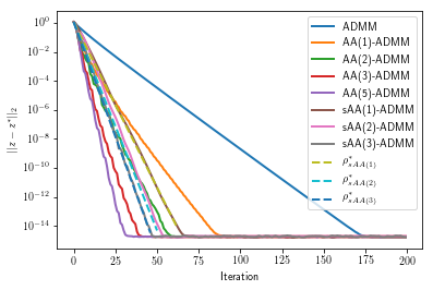
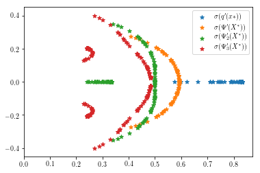
Figure 1: Ridge regression. (top) Comparison of error reduction using ADMM, AA($m$)-ADMM and sAA($m$)-ADMM. (bottom) Spectrum of $\mathbf{q}^{\prime}$ of ADMM, $\mathbf{\Psi}^{\prime}$ of sAA(1)-ADMM, and $\mathbf{\Psi}_{2}^{\prime}$ and $\mathbf{\Psi}_{3}^{\prime}$ of sAA(2)-ADMM and sAA(3)-ADMM.

3.1.3 Convergence results

We obtain convergence plots for the error $\|\mathbf{z}-\mathbf{z}^{*}\|_{2}$ as shown in Figure 1 (top). We see that ADMM converges linearly. The convergence factor of ADMM is substantially improved by the AA-based methods. AA(2) and AA(3) converge slightly faster than AA(1), and sAA(1) converges with similar asymptotic speed.

The convergence improvement of the AA-ADMM methods over ADMM can be understood in terms of spectral properties as follows. Figure 1 (bottom) shows the spectrum of the ADMM iteration matrix $\mathbf{M}$, $\sigma(\mathbf{M})\in(0,1)$. The spectrum is real since $\mathbf{M}$ is symmetric, and the spectral radius $\rho^{*}_{q^{\prime}}=0.833.$ Therefore, according to 3, the optimal $\beta$ for sAA(1) is

$$\beta^{*}=\frac{1-\sqrt{1-\rho^{*}_{q^{\prime}}}}{1+\sqrt{1-\rho^{*}_{q^{\prime}}}}=0.420.$$

The corresponding optimal sAA(1) linear convergence factor is

$$\rho^{*}_{sAA(1)-ADMM}=\rho(\mathbf{\Psi}^{\prime})=1-\sqrt{1-\rho^{*}_{q^{\prime}}}=0.592<0.833.$$

The approximately optimal $\beta_{1}^{*}$ and $\beta_{2}^{*}$ for sAA(2) are

$$\beta_{1}^{*}=0.70,\;\beta_{2}^{*}=-0.10,$$

with sAA(2) linear convergence factor

$$\rho^{*}_{sAA(2)-ADMM}=\rho(\mathbf{\Psi}_{2}^{\prime})=0.516.$$

Similarly, for sAA(3), we obtain

$$\beta_{1}^{*}=0.955,\;\beta_{2}^{*}=-0.250,\;\beta_{3}^{*}=0.028,$$

with sAA(3) linear convergence factor

$$\rho^{*}_{sAA(3)-ADMM}=\rho(\mathbf{\Psi}_{3}^{\prime})=0.4837<\rho(\mathbf{\Psi}_{2}^{\prime})<\rho(\mathbf{\Psi}^{\prime})<\rho^{*}_{q^{\prime}}.$$

Figure 1 (bottom) also shows the spectrum of the sAA(1)-ADMM iteration matrix, $\mathbf{\Psi}^{\prime}$, and of the sAA(2)-ADMM and sAA(3)-ADMM iteration matrices, $\mathbf{\Psi}_{2}^{\prime}$ and $\mathbf{\Psi}_{3}^{\prime}$. The acceleration methods spread the ADMM spectrum out in the complex plane in a way that strongly reduces the asymptotic convergence factor: e.g., $\rho(\mathbf{\Psi}^{\prime})$ is much smaller than $\rho^{*}_{q^{\prime}}$. Note that stationary iterative method (14) maps part of the nonnegative real spectrum of $\mathbf{q}^{\prime}(\mathbf{x}^{*})$ to a circle, according to 1. As seen in Figure 1 (top), the optimal sAA(1)-ADMM factor, $\rho^{*}_{sAA(1)-ADMM}$, provides a useful prediction of the convergence factors of the AA-ADMM methods. The convergence speed of sAA(1)-ADMM matches the theoretical prediction of $\rho^{*}_{sAA(1)-ADMM}$.

3.2 Regularized logistic regression (see, e.g., boyd2011distributed ; nonlinear and smooth problem)

3.2.1 Problem description

We consider a simple logistic regression model in this section. The objective function of the regularized logistic regression model is

$$\min_{\mathbf{x}}\frac{1}{m}\sum_{i=1}^{m}\log(1+\exp(-y_{i}(\mathbf{a}_{i}^{T}\mathbf{w}+\mathbf{c}))+\lambda||\mathbf{x}||_{2}^{2},$$

where

$$A=\begin{bmatrix}\mathbf{a}_{1}^{T}\\ \vdots\\ \mathbf{a}_{m}^{T}\end{bmatrix}\in\mathbb{R}^{m\times n},$$

are $m$ data samples, $y_{1},\cdots,y_{m}$ are the corresponding labels, and

$$\mathbf{x}=\begin{bmatrix}\mathbf{c}\\ \mathbf{w}\end{bmatrix},\quad\mathbf{w}\in\mathbb{R}^{n},\quad\mathbf{c}\in\mathbb{R},$$

are the linear combination coefficients and bias to be optimized. To apply ADMM, we write this problem as

$$\min_{\mathbf{x},\mathbf{z}}\; \frac{1}{m}\sum_{i=1}^{m}\log(1+\exp(-y_{i}(\mathbf{a}_{i}^{T}\mathbf{w}+\mathbf{c})))+\lambda||\mathbf{z}||_{2}^{2},$$

s.t. $$\mathbf{x}-\mathbf{z}=0.$$

This gives the augmented Lagrangian

$$L(\mathbf{x},\mathbf{z},\mathbf{u},\rho)=\frac{1}{m}\sum_{i=1}^{m}\log(1+\exp(-y_{i}(\mathbf{a}_{i}^{T}\mathbf{w}+\mathbf{c})))+\lambda||\mathbf{z}||_{2}^{2}+\frac{\rho}{2}||\mathbf{x}-\mathbf{z}+\mathbf{u}||_{2}^{2}-\frac{\rho}{2}||\mathbf{u}||_{2}^{2}.$$

Hence, we get the ADMM steps

$$\begin{cases}\mathbf{x}_{k+1}=\text{argmin}_{\mathbf{x}}\frac{1}{m}\sum_{i=1}^{m}\log(1+\exp(-y_{i}(\mathbf{a}_{i}^{T}\mathbf{w}+\mathbf{c})))+\frac{\rho}{2}||\mathbf{x}-\mathbf{z}_{k}+\mathbf{u}_{k}||_{2}^{2},\\ \mathbf{z}_{k+1}=\text{argmin}_{\mathbf{z}}\lambda||\mathbf{z}||_{2}^{2}+\frac{\rho}{2}||\mathbf{x}_{k+1}-\mathbf{z}+\mathbf{u}_{k}||_{2}^{2},\\ \mathbf{u}_{k+1}=\mathbf{u}_{k}+\mathbf{x}_{k+1}-\mathbf{z}_{k+1}.\end{cases}$$

To solve for $\mathbf{x}_{k+1}$, we use Newton’s method.

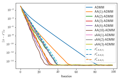
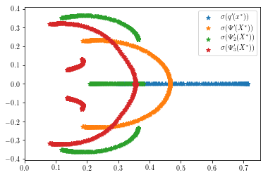
Figure 2: $l_{2}$-regularized logistic regression. (top) Comparison of error reduction using ADMM, AA($m$)-ADMM and sAA($m$)-ADMM. (bottom) Spectrum of $\mathbf{q}^{\prime}$ of ADMM, $\mathbf{\Psi}^{\prime}$ of sAA(1)-ADMM, and $\mathbf{\Psi}_{2}^{\prime}$ and $\mathbf{\Psi}_{3}^{\prime}$ of sAA(2)-ADMM and sAA(3)-ADMM.

3.2.2 Parameters for the test problem

For this problem, we applied our algorithms to the Madelon data set from the UCI machine learning repository. To reduce the amount of computation, we only used a portion of the features and examples. The regularization parameter is $\lambda=2$, and the augmented Lagrangian penalty parameter is $\rho=10$.

3.2.3 Convergence results

Since the FPI representation of ADMM for solving the regularized logistic regression problem is nonlinear, we are now not able to find an explicit expression for $\mathbf{z}_{k+1}=\mathbf{q}(\mathbf{z}_{k})$ like before. To determine the spectrum of $\mathbf{q}^{\prime}(\mathbf{z}^{*})$, we use the first-order finite difference method with step size $h=1\times 10^{-4}$ to approximate $\mathbf{q}^{\prime}(\mathbf{z}^{*})$ at the approximate true solution solved to $10^{-16}$ accuracy.

Figure 2 (top) compares the error norm reduction when using ADMM, AA($m$)-ADMM and sAA($m$)-ADMM. The convergence acceleration seen in the figure can be explained based on the spectra in Figure 2 (bottom). The spectrum of $\mathbf{q}^{\prime}(\mathbf{z}^{*})$ has asymptotic convergence factor $\rho^{*}_{q^{\prime}}=0.714$. We can choose the optimal $\beta^{*}$ the same way as in the ridge regression problem:

$$\beta^{*}=\frac{1-\sqrt{1-\rho^{*}_{q^{\prime}}}}{1+\sqrt{1-\rho^{*}_{q^{\prime}}}}=0.303.$$

The corresponding optimal sAA(1)-ADMM linear convergence factor is

$$\rho^{*}_{sAA(1)-ADMM}=\rho(\mathbf{\Psi}^{\prime})=1-\sqrt{1-\rho^{*}_{q^{\prime}}}=0.465<(\rho^{*}_{q^{\prime}})^{2}.$$

The approximately optimal $\beta_{1}^{*}$ and $\beta_{2}^{*}$ for sAA(2) are

$$\beta_{1}^{*}=0.65,\;\beta_{2}^{*}=-0.10,$$

with sAA(2) linear convergence factor

$$\rho^{*}_{sAA(2)-ADMM}=\rho(\mathbf{\Psi}_{2}^{\prime})=0.450.$$

Similarly, for sAA(3), we obtain

$$\beta_{1}^{*}=0.61,\;\beta_{2}^{*}=-0.115,\;\beta_{3}^{*}=0.009,$$

with sAA(3) linear convergence factor

$$\rho^{*}_{sAA(3)-ADMM}=\rho(\mathbf{\Psi}_{3}^{\prime})=0.364.$$

Figure 2 (top) shows that $\rho^{*}_{sAA(m)-ADMM}$ is a useful prediction for the convergence factors of the AA-accelerated ADMM methods.

3.3 Total variation (see, e.g., boyd2011distributed ; nonlinear and nonsmooth problem, complex spectrum)

3.3.1 Problem description

The total variation model is a widely used method for applications like image denoising. The optimization problem is

$$\min_{\mathbf{x}}\frac{1}{2}||\mathbf{y}-\mathbf{x}||_{2}^{2}+\alpha||\mathbf{D}\mathbf{x}||_{1}^{2},$$

where $\mathbf{x}\in\mathbb{R}^{n}$ is the variable, $\mathbf{y}\in\mathbb{R}^{n}$ is the problem data (e.g. image pixel values), $\alpha>0$ is a smoothing parameter, and $\mathbf{D}\in\mathbb{R}^{(n-1)\times n}$ is the difference operator

$$\mathbf{D}=\begin{bmatrix}-1&1\\ &-1&1\\ &&\ddots&\ddots\\ &&&-1&1\end{bmatrix}.$$

To use ADMM, we write this problem as

$$\min_{\mathbf{x},\mathbf{z}}\; \frac{1}{2}||\mathbf{y}-\mathbf{x}||_{2}^{2}+\alpha||\mathbf{z}||_{1}^{2},$$

s.t. $$\mathbf{D}\mathbf{x}-\mathbf{z}=0.$$

The augmented Lagrangian is

$$L_{\rho}(\mathbf{x},\mathbf{z},\mathbf{u})=\frac{1}{2}||\mathbf{y}-\mathbf{x}||_{2}^{2}+\alpha||\mathbf{z}||_{1}^{2}+\frac{\rho}{2}||\mathbf{D}\mathbf{x}-\mathbf{z}+\mathbf{u}||_{2}^{2}-\frac{\rho}{2}||\mathbf{u}||_{2}^{2}.$$

The ADMM steps for this problem are:

$$\begin{cases}\mathbf{x}_{k+1}=\text{argmin}_{\mathbf{x}}\frac{1}{2}||\mathbf{y}-\mathbf{x}||_{2}^{2}+\frac{\rho}{2}||\mathbf{D}\mathbf{x}-\mathbf{z}_{k}+\mathbf{u}_{k}||_{2}^{2},\\ \mathbf{z}_{k+1}=\text{argmin}_{\mathbf{z}}\alpha||\mathbf{z}||_{1}^{2}+\frac{\rho}{2}||\mathbf{D}\mathbf{x}_{k+1}+\mathbf{u}_{k}-\mathbf{z}||_{2}^{2},\\ \mathbf{u}_{k+1}=\mathbf{u}_{k}+\mathbf{D}\mathbf{x}_{k+1}-\mathbf{z}_{k+1},\end{cases}$$

where $\mathbf{x}_{k+1}$ is the proximal operator of the $l_{2}$ norm which can be evaluated from a least squares problem as before,

$$\mathbf{x}_{k+1}=\text{argmin}_{\mathbf{x}}\left|\left|\begin{bmatrix}\mathbf{D}\\ \frac{1}{\sqrt{\rho}}\mathbf{I}\end{bmatrix}x-\begin{bmatrix}\mathbf{z}_{k}-\mathbf{u}_{k}\\ \frac{1}{\sqrt{\rho}}\mathbf{y}\end{bmatrix}\right|\right|_{2}^{2},$$

and $\mathbf{z}^{k+1}$ is just the proximal operator of the $l_{1}$-norm,

$$\mathbf{z}_{k+1}=\text{prox}_{\frac{\alpha}{\rho}||\cdot||_{1}}(\mathbf{D}\mathbf{x}_{k+1}+\mathbf{u}_{k}).$$

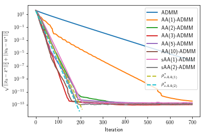
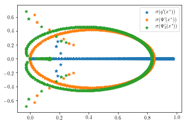
Figure 3: Total variation. (top) Comparison of error reduction using ADMM, AA($m$)-ADMM and sAA($m$)-ADMM. (bottom) Spectrum of ADMM iteration matrix $\mathbf{q}^{\prime}$ and sAA($1$)-ADMM iteration matrix $\mathbf{\Psi}^{\prime}$.

3.3.2 Parameters for the test problem

We test our algorithms on randomly generated data $\mathbf{y}$ of size $1000$ sampled from the standard normal distribution. The smoothing parameter is $\alpha=0.001\cdot||\mathbf{y}||_{\infty}$. For the penalty parameter, we use $\rho=10$.

3.3.3 Convergence results

We use the first-order finite difference method with step size $h=1\times 10^{-5}$ to approximate $\mathbf{q}^{\prime}(\mathbf{z}^{*},\mathbf{u}^{*})$ at the approximate true solution solved to $10^{-16}$ accuracy.

Figure 3 (top) compares the error norm reduction when using ADMM, AA($m$)-ADMM and sAA($m$)-ADMM. The convergence acceleration seen in the figure can be explained based on the spectra in Figure 3 (bottom). The spectrum of $\mathbf{q}^{\prime}(\mathbf{z}^{*},\mathbf{u}^{*})$ has asymptotic convergence factor $\rho^{*}_{q^{\prime}}=0.976$. The spectrum has some complex eigenvalues. We choose $\beta^{*}$ according to 4,

$$\beta^{*}=\frac{1-\sqrt{1-\rho^{*}_{q^{\prime}}}}{1+\sqrt{1-\rho^{*}_{q^{\prime}}}}=0.730.$$

The corresponding lower bound on the optimal sAA(1)-ADMM linear convergence factor is

$$\rho^{*}_{sAA(1)-ADMM}\leq 1-\sqrt{1-\rho^{*}_{q^{\prime}}}=0.844.$$

The spectral radius of the numerically computed $\Psi^{\prime}$ using $\beta^{*}$ is given by

$$\rho_{sAA(1)-ADMM}(\beta^{*})=\rho(\mathbf{\Psi}^{\prime}(\beta^{*}))=0.844<(\rho^{*}_{q^{\prime}})^{2},$$

which is numerically equal to the lower bound. It is interesting to note that it was observed numerically in desterck2020 that, for the case of sAA(1) acceleration of Alternating Least Squares for canonical tensor decomposition, for which $\mathbf{q}^{\prime}(\mathbf{x}^{*})$ has a complex spectrum, the lower bound in 4 is always achieved.

Finally, the approximately optimal $\beta_{1}^{*}$ and $\beta_{2}^{*}$ for sAA(2) are

$$\beta_{1}^{*}=0.95,\;\beta_{2}^{*}=-0.10,$$

with sAA(2) linear convergence factor

$$\rho^{*}_{sAA(2)-ADMM}=\rho(\mathbf{\Psi}_{2}^{\prime})=0.832.$$

3.4 Lasso problem (see, e.g., boyd2011distributed ; nonlinear and nonsmooth problem, complex spectrum)

3.4.1 Problem description

$l_{1}$-regularized linear regression is also called the lasso problem:

$$\min_{\mathbf{x}}\; \frac{1}{2}||\mathbf{A}\mathbf{x}-\mathbf{b}||_{2}^{2}+\lambda||\mathbf{x}||_{1},$$

where $\mathbf{A}\in\mathbb{R}^{m\times n}$ and $\mathbf{b}\in\mathbb{R}^{m}$ are given data, $\lambda>0$ is a scalar regularization parameter, and $\mathbf{x}\in\mathbb{R}^{n}$ is the optimization variable. In typical applications, there are many more features than training examples, and the goal is to find a parsimonious model for the data boyd2011distributed .

To apply ADMM, we solve the following constrained problem

$$\min_{\mathbf{x},\mathbf{z}}\; \frac{1}{2}||\mathbf{A}\mathbf{x}-\mathbf{b}||_{2}^{2}+\lambda||\mathbf{z}||_{1},$$

s.t. $$\mathbf{x}-\mathbf{z}=0.$$

The scaled augmented Lagrangian is

$$L_{\rho}(\mathbf{x},\mathbf{z},\mathbf{u})=\frac{1}{2}||\mathbf{A}\mathbf{x}-\mathbf{b}||_{2}^{2}+\lambda||\mathbf{z}||_{1}+\frac{\rho}{2}||\mathbf{x}-\mathbf{z}+\mathbf{u}||_{2}^{2}-\frac{\rho}{2}||\mathbf{u}||_{2}^{2}.$$

Therefore, we get the ADMM steps

$$\begin{cases}\mathbf{x}_{k+1}=\text{argmin}_{\mathbf{x}}\frac{1}{2}||\mathbf{A}\mathbf{x}-\mathbf{b}||_{2}^{2}+\frac{\rho}{2}||\mathbf{x}-\mathbf{z}_{k}+\mathbf{u}_{k}||_{2}^{2}\\ \mathbf{z}_{k+1}=\text{argmin}_{\mathbf{z}}\lambda||\mathbf{z}||_{1}+\frac{\rho}{2}||\mathbf{x}_{k+1}-\mathbf{z}+\mathbf{u}_{k}||_{2}^{2}\\ \mathbf{u}_{k+1}=\mathbf{u}_{k}+\mathbf{x}_{k+1}-\mathbf{z}_{k+1},\end{cases}$$

which gives

$$\begin{cases}\mathbf{x}_{k+1}=(\mathbf{A}^{T}\mathbf{A}+\rho\mathbf{I})^{-1}\left(\mathbf{A}^{T}\mathbf{b}+\rho(\mathbf{z}_{k}-\mathbf{u}_{k})\right)\\ \mathbf{z}_{k+1}=\text{prox}_{\frac{\lambda}{\rho}||\cdot||_{1}}(\mathbf{x}_{k+1}+\mathbf{u}_{k}),\\ \mathbf{u}_{k+1}=\mathbf{u}_{k}+\mathbf{x}_{k+1}-\mathbf{z}_{k+1},\end{cases}$$

where $\mathbf{x}_{k+1}$ can be solved efficiently as a least squares problem like in ridge regression. Since the update of $\mathbf{z}_{k+1}$ is nonsmooth, $\mathbf{u}_{k+1}$ cannot be expressed explicitly as a function of $\mathbf{z}_{k+1}$, and we will treat one ADMM iteration as a FPI about both variables $\mathbf{z}$ and $\mathbf{u}$ in order to apply Anderson acceleration.

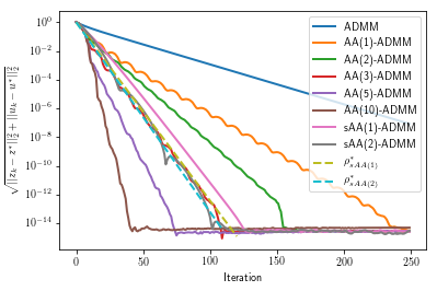
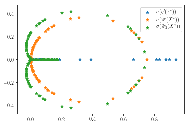
Figure 4: Lasso problem (density = 0.001). (top) comparison of error reduction using ADMM, sAA($m$)-ADMM and AA($m$)-ADMM. (bottom) Spectrum of $\mathbf{q}^{\prime}$ of ADMM, $\mathbf{\Psi}^{\prime}$ of sAA(1)-ADMM, and $\mathbf{\Psi}_{2}^{\prime}$ of sAA(2)-ADMM.

3.4.2 Parameters for the test problem

We test our algorithms on a randomly generate sparse matrix of size $m\times n=150\times 300$ with density 0.001 and 0.01 respectively, sampled from the uniform distribution on [0,1). The $\mathbf{b}$ vector is sampled from the standard normal distribution. The regularization parameter $\lambda=1$, and we pick the penalty parameter $\rho=10$.

3.4.3 Convergence results

Since now the FPI is about variables $\mathbf{z}$ and $\mathbf{u}$, we will accelerate the stacked variable $[\mathbf{z};\mathbf{u}]$. The error norm during the iteration is evaluated as

$$\mathbf{e}_{k}=\sqrt{||\mathbf{z}_{k}-\mathbf{z}^{*}||_{2}^{2}+||\mathbf{u}_{k}-\mathbf{u}^{*}||_{2}^{2}}.$$

We use the first-order finite difference method with step size $h=0.001$ to approximate $\mathbf{q}^{\prime}(\mathbf{z}^{*},\mathbf{u}^{*})$ at the approximate true solution solved to $10^{-16}$ accuracy.

Figure 4 (top) compares the error norm reduction when using ADMM, AA($m$)-ADMM and sAA($m$)-ADMM for the case when the data matrix density is 0.001. The convergence acceleration seen in the figure can be explained based on the spectra in Figure 4 (bottom). The spectrum of $\mathbf{q}^{\prime}(\mathbf{z}^{*})$ has asymptotic convergence factor $\rho^{*}_{q^{\prime}}=0.938$. We can choose the optimal $\beta^{*}$ the same way as in the ridge regression problem,

$$\beta^{*}=\frac{1-\sqrt{1-\rho^{*}_{q^{\prime}}}}{1+\sqrt{1-\rho^{*}_{q^{\prime}}}}=0.601.$$

The corresponding optimal sAA(1)-ADMM linear convergence factor is

$$\rho^{*}_{sAA(1)-ADMM}=\rho(\mathbf{\Psi}^{\prime})=1-\sqrt{1-\rho^{*}_{q^{\prime}}}=0.751<(\rho^{*}_{q^{\prime}})^{2}.$$

The approximately optimal $\beta_{1}^{*}$ and $\beta_{2}^{*}$ for sAA(2) are

$$\beta_{1}^{*}=0.85,\;\beta_{2}^{*}=-0.10,$$

with sAA(2) linear convergence factor

$$\rho^{*}_{sAA(2)-ADMM}=\rho(\mathbf{\Psi}_{2}^{\prime})=0.737.$$

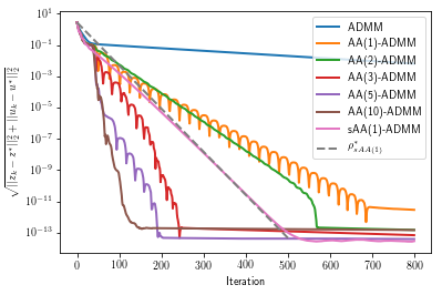
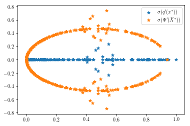
Figure 5: Lasso problem (density = 0.01). (top) Comparison of error reduction using ADMM, sAA($m$)-ADMM and AA($m$)-ADMM. (bottom) Spectrum of ADMM iteration matrix $\mathbf{q}^{\prime}$ and sAA($1$)-ADMM iteration matrix $\mathbf{\Psi}^{\prime}$.

3.4.4 $\mathbf{q}^{\prime}(\mathbf{x})$ with complex eigenvalues

Note that in the lasso test of Figure 4, the eigenvalues of $\mathbf{q}^{\prime}(\mathbf{x}^{*})$ happen to be all real. However, this is not the case if we increase the sparsity density of data matrix $A$. For example, for a density of 0.01, $\mathbf{q}^{\prime}(\mathbf{z}^{*})$ has a few complex eigenvalues as shown in Figure 5 (bottom), where $\rho^{*}_{q^{\prime}}=0.996$. For this case, numerical results comparing the convergence of different algorithms are shown in Figure 5 (top). The value of $\beta^{*}$ we use is chosen according to 4,

$$\beta^{*}=\frac{1-\sqrt{1-\rho^{*}_{q^{\prime}}}}{1+\sqrt{1-\rho^{*}_{q^{\prime}}}}=0.884.$$

The corresponding sAA(1)-ADMM linear convergence factor is

$$\rho^{*}_{sAA(1)-ADMM}=\rho(\mathbf{\Psi}^{\prime})=1-\sqrt{1-\rho^{*}_{q^{\prime}}}=0.938<(\rho^{*}_{q^{\prime}})^{2}.$$

It is interesting to consider the situation when $\mathbf{q}^{\prime}(\mathbf{x}^{*})$ has complex eigenvalues with large imaginary part. Let $\mu_{+}$ be the largest nonnegative real eigenvalue of $\mathbf{q}^{\prime}(\mathbf{x}^{*})$. It is easy to show that, if the equality $\rho^{*}_{sAA(1)}=1-\sqrt{1-\rho^{*}_{q^{\prime}}}$ holds in 4 with $\rho^{*}_{q^{\prime}}=\mu_{+}$ and $\beta^{*}=\frac{1-\sqrt{1-\rho^{*}_{q^{\prime}}}}{1+\sqrt{1-\rho^{*}_{q^{\prime}}}}$, then the rightmost point of the circle of 1 is the image of $\mu_{+}$ under the mapping from $\mu$ to $\lambda$ defined by (15), and this point determines $\rho(\mathbf{\Psi}^{\prime})=\rho^{*}_{sAA(1)}$. According to Corollary S.1 in the supplementary materials of desterck2020 , this also holds when $\rho^{*}_{q^{\prime}}>\mu_{+}$ and $\rho^{*}_{sAA(1)}=1-\sqrt{1-\mu_{+}}$, with $\beta^{*}=\frac{1-\sqrt{1-\mu_{+}}}{1+\sqrt{1-\mu_{+}}}$. In these cases, the spectral radius of $\mathbf{\Psi}^{\prime}$ for sAA(1) with optimal weight is determined by the mapped eigenvalue of $\mu_{+}$, which is the rightmost point of the circle, and the complex eigenvalues of $\mathbf{q}^{\prime}(\mathbf{x}^{*})$ do not influence $\rho(\mathbf{\Psi}^{\prime})$. However, when $\mathbf{q}^{\prime}(\mathbf{x}^{*})$ has complex eigenvalues with large imaginary part, these eigenvalues may be mapped to eigenvalues $\lambda$ of $\mathbf{\Psi}^{\prime}$ that are sufficiently far outside the circle of 1 to determine the spectral radius of $\mathbf{\Psi}^{\prime}$. In this case, we cannot determine the optimal $\beta^{*}$ and $\rho^{*}_{sAA(1)}$ by the expressions (with equality) in 4 or Corollary S.1 in the supplementary materials of desterck2020 . We now give an example demonstrating this. We consider the lasso example with density = 0.06. Figure 6 (bottom) plots the distribution of eigenvalues for both $\mathbf{q}^{\prime}(\mathbf{z}^{*},\mathbf{u}^{*})$ and $\mathbf{\Psi}^{\prime}$, where we have used $\beta=\frac{1-\sqrt{1-\rho^{*}_{q^{\prime}}}}{1+\sqrt{1-\rho^{*}_{q^{\prime}}}}$ in sAA(1)-ADMM. We can see that the largest eigenvalues of $\mathbf{\Psi}^{\prime}$ induced by complex eigenvalues of $\mathbf{q}^{\prime}$ (those that are not lying on the circle) have a larger modulus (=0.944) than the largest-size eigenvalue induced by the real eigenvalues of $\mathbf{q}^{\prime}$, which is of size $1-\sqrt{1-\rho^{*}_{q^{\prime}}}=0.848$ (since for this example it still holds that $\rho^{*}_{q^{\prime}}=\mu_{+}$). Hence, complex eigenvalues of $\mathbf{q}^{\prime}$ dominate the spectrum of $\mathbf{\Psi}^{\prime}$ and the equality in 4 does not hold, since it requires that the largest-size eigenvalue of $\mathbf{\Psi}^{\prime}$ comes from real eigenvalues of $\mathbf{q}^{\prime}$. This observation matches with the numerical results shown in Figure 6 (top), where the convergence of the sAA(1) algorithm using $\beta=(1-\sqrt{1-\rho^{*}_{q^{\prime}}})/(1+\sqrt{1-\rho^{*}_{q^{\prime}}})$ from 4 does not match the convergence factor $1-\sqrt{1-\rho^{*}_{q^{\prime}}}$ that would correspond to 4 if equality were to hold. (Note that for the previous test with density 0.01 we do get a close match (see Figure 5 (top)).) We note that in a case like the one from Figure 6, sAA(1) may generate divergent results when using $\beta=(1-\sqrt{1-\rho^{*}_{q^{\prime}}})/(1+\sqrt{1-\rho^{*}_{q^{\prime}}})$ since this is not the correct optimal $\beta^{*}$. Finding the optimal coefficient $\beta^{*}$ for sAA(1) in this scenario is an open question that needs more investigation.

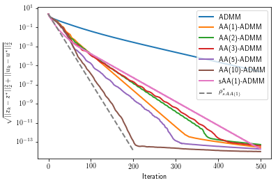
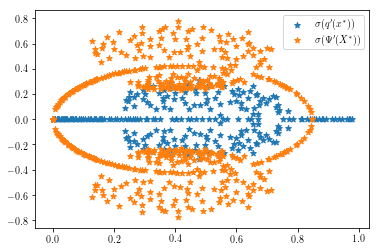
Figure 6: Lasso problem (density = 0.06). (top) Comparison of error reduction using ADMM, sAA($m$)-ADMM and AA($m$)-ADMM. (bottom) Spectrum of ADMM iteration matrix $\mathbf{q}^{\prime}$ and sAA($1$)-ADMM iteration matrix $\mathbf{\Psi}^{\prime}$.

3.5 Nonnegative least squares (see, e.g., fu2019anderson ; nonlinear problem with inequality constraint)

3.5.1 Problem description

The nonnegative least squares problem is

$$\min_{\mathbf{x}}||\mathbf{F}\mathbf{x}-\mathbf{g}||_{2}^{2},\quad\text{s.t.}\quad\mathbf{x}\geq 0,$$

where $\mathbf{x}\in\mathbb{R}^{n}$ is the variable, and $\mathbf{F}\in\mathbb{R}^{m\times n}$ and $\mathbf{g}\in\mathbb{R}^{m}$ are problem data. We can integrate the nonnegativity constraint into the objective function and rewrite the problem as

$$\min_{\mathbf{x},\mathbf{z}}\; ||\mathbf{F}\mathbf{x}-\mathbf{g}||_{2}^{2}+\mathcal{I}_{\mathbb{R}_{+}^{n}}(\mathbf{z}),$$

s.t. $$\mathbf{x}-\mathbf{z}=0,$$

where $\mathcal{I}_{\mathbb{R}_{+}^{n}}$ is the indicator function defined as

$$\mathcal{I}_{\mathbb{R}_{+}^{n}}(\mathbf{z})=\begin{cases}0,&\mathbf{z}\geq 0\\ +\infty,&\text{otherwise}.\end{cases}$$

The scaled augmented Lagrangian of this problem is

$$L_{\rho}(\mathbf{x},\mathbf{z},\mathbf{u})=||\mathbf{F}\mathbf{x}-\mathbf{g}||_{2}^{2}+\mathcal{I}_{\mathbb{R}_{+}^{n}}(\mathbf{z})+\frac{\rho}{2}||\mathbf{x}-\mathbf{z}+\mathbf{u}||_{2}^{2}-\frac{\rho}{2}||\mathbf{u}||_{2}^{2}.$$

The ADMM steps on this problem are:

$$\begin{cases}\mathbf{x}_{k+1}=\text{argmin}_{\mathbf{x}}||\mathbf{F}\mathbf{x}-\mathbf{g}||_{2}^{2}+\frac{\rho}{2}||\mathbf{x}-\mathbf{z}_{k}+\mathbf{u}_{k}||_{2}^{2}\\ \mathbf{z}_{k+1}=\text{argmin}_{\mathbf{z}}\mathcal{I}_{\mathbb{R}_{+}^{n}}(\mathbf{z})+\frac{\rho}{2}||\mathbf{x}_{k+1}+\mathbf{u}_{k}-\mathbf{z}||_{2}^{2}\\ \mathbf{u}_{k+1}=\mathbf{u}_{k}+\mathbf{x}_{k+1}-\mathbf{z}_{k+1}\end{cases}$$

where the first step for $\mathbf{x}_{k+1}$ is the proximal operator of the $l_{2}$-norm. The second step is just the proximal operator of the indicator function, which is equivalent to the projection operator

$$\mathbf{z}_{k+1}=\frac{1}{\rho}\Uppi_{\mathbb{R}_{+}^{n}}(\mathbf{x}_{k+1}+u_{k}).$$

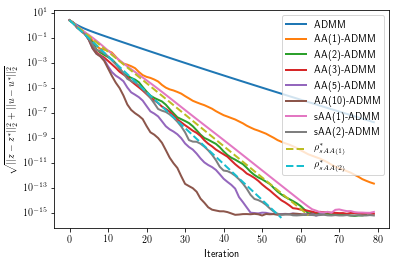
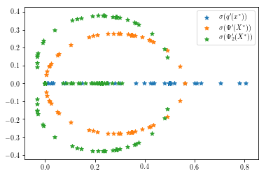
Figure 7: Nonnegative least squares. (top) Comparison of error reduction using ADMM, sAA($m$)-ADMM and AA($m$)-ADMM. (bottom) Spectrum of $\mathbf{q}^{\prime}$ of ADMM, $\mathbf{\Psi}^{\prime}$ of sAA(1)-ADMM, and $\mathbf{\Psi}_{2}^{\prime}$ of sAA(2)-ADMM.

3.5.2 Parameters for the test problem

We test our algorithms on a randomly generated sparse matrix of size $m\times n=150\times 300$ with density 0.001, sampled from the standard normal distribution. The $g$ vector is sampled from the standard normal distribution. The augmented Lagrangian penalty parameter is $\rho=2$.

3.5.3 Convergence results

We use the first-order finite difference method with step size $h=0.001$ to approximate $\mathbf{q}^{\prime}(\mathbf{z}^{*},\mathbf{u}^{*})$ at the approximate true solution solved to $10^{-16}$ accuracy.

Figure 7 (top) compares the error norm reduction when using ADMM, AA($m$)-ADMM and sAA($m$)-ADMM. The convergence acceleration seen in the figure can be explained based on the spectra in Figure 7 (bottom). The spectrum of $\mathbf{q}^{\prime}(\mathbf{z}^{*},\mathbf{u}^{*})$ has asymptotic convergence factor $\rho^{*}_{q^{\prime}}=0.806$. We can choose the optimal $\beta^{*}$ the same way as in the ridge regression problem

$$\beta^{*}=\frac{1-\sqrt{1-\rho^{*}_{q^{\prime}}}}{1+\sqrt{1-\rho^{*}_{q^{\prime}}}}=0.389.$$

The corresponding optimal sAA(1)-ADMM linear convergence factor is

$$\rho^{*}_{sAA(1)-ADMM}=\rho(\mathbf{\Psi}^{\prime})=1-\sqrt{1-\rho^{*}_{q^{\prime}}}=0.560<(\rho^{*}_{q^{\prime}})^{2}.$$

The approximately optimal $\beta_{1}^{*}$ and $\beta_{2}^{*}$ for sAA(2) are

$$\beta_{1}^{*}=0.70,\;\beta_{2}^{*}=-0.10,$$

with sAA(2) linear convergence factor

$$\rho^{*}_{sAA(2)-ADMM}=\rho(\mathbf{\Psi}_{2}^{\prime})=0.516.$$

3.6 Constrained logistic regression (see, e.g., mai2019anderson ; nonlinear problem with box constraint)

3.6.1 Problem description

The constrained regularized logistic regression adds a constraint on $||\mathbf{x}||_{\infty}$ to the regularized logistic regression problem that we have already discussed:

$$\min_{\mathbf{x}}\; \frac{1}{m}\sum_{i=1}^{m}\log(1+\exp(-y_{i}(\mathbf{a}_{i}^{T}\mathbf{w}+\mathbf{c})))+\lambda||\mathbf{x}||_{2}^{2},$$

s.t. $$||\mathbf{x}||_{\infty}\leq 1.$$

To apply ADMM, we rewrite this problem as

$$\min_{\mathbf{x},\mathbf{z}}\; \frac{1}{m}\sum_{i=1}^{m}\log(1+\exp(-y_{i}(a_{i}^{T}\mathbf{w}+\mathbf{c})))+\lambda||\mathbf{x}||_{2}^{2}+\mathcal{I}_{\Omega}(\mathbf{z}),$$

s.t. $$\mathbf{x}-\mathbf{z}=0,$$

where $\Upomega=\{\mathbf{x}:||\mathbf{x}||_{\infty}\leq 1\}$. This gives the augmented Lagrangian

$$L_{\rho}(\mathbf{x},\mathbf{z},\mathbf{u})=\frac{1}{m}\sum_{i=1}^{m}\log(1+\exp(-y_{i}(\mathbf{a}_{i}^{T}\mathbf{w}+\mathbf{c})))+\lambda||\mathbf{x}||_{2}^{2}+\mathcal{I}_{\Omega}(\mathbf{z})+\frac{\rho}{2}||\mathbf{x}-\mathbf{z}+\mathbf{u}||_{2}^{2}-\frac{\rho}{2}||\mathbf{u}||_{2}^{2}.$$

Hence, we get the ADMM steps

$$\begin{cases}\mathbf{x}_{k+1}=\text{argmin}_{\mathbf{x}}\frac{1}{m}\sum_{i=1}^{m}\log(1+\exp(-y_{i}(\mathbf{a}_{i}^{T}\mathbf{w}+\mathbf{c})))+\lambda||\mathbf{x}||_{2}^{2}+\frac{\rho}{2}||\mathbf{x}-\mathbf{z}_{k}+\mathbf{u}_{k}||_{2}^{2}\\ \mathbf{z}_{k+1}=\text{argmin}_{\mathbf{z}}\mathcal{I}_{\Omega}(\mathbf{z})+\frac{\rho}{2}||\mathbf{x}_{k+1}-\mathbf{z}+\mathbf{u}_{k}||_{2}^{2}\\ \mathbf{u}_{k+1}=\mathbf{u}_{k}+\mathbf{x}_{k+1}-\mathbf{z}_{k+1}.\end{cases}$$

Like before, we use Newton’s method to solve for $\mathbf{x}_{k+1}$. For $\mathbf{z}_{k+1}$, since the proximal operation of an indicator function is just a projection, we have

$$\mathbf{z}_{k+1}=\frac{1}{\rho}\Uppi_{\Upomega}(\mathbf{x}_{k+1}+\mathbf{u}_{k}),$$

which is

$$[\mathbf{z}_{k+1}]_{j}=\begin{cases}\frac{1}{\rho},&[\mathbf{x}_{k+1}+\mathbf{u}_{k}]_{j}\in[1,\infty)\\ \frac{1}{\rho}[\mathbf{x}_{k+1}+\mathbf{u}_{k}]_{j},&[\mathbf{x}_{k+1}+\mathbf{u}_{k}]_{j}\in(-1,1)\\ -\frac{1}{\rho},&[\mathbf{x}_{k+1}+\mathbf{u}_{k}]_{j}\in(-\infty,-1].\end{cases}$$

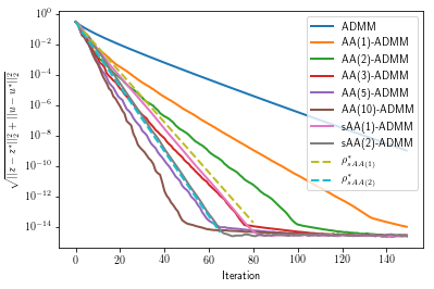
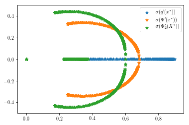
Figure 8: Constrained regularized logistic regression. (top) Comparison of error reduction using ADMM, sAA($m$)-ADMM and AA($m$)-ADMM. (bottom) Spectrum of ADMM iteration matrix $\mathbf{q}^{\prime}_{*}$ and sAA($1$)-ADMM iteration matrix $\mathbf{\Psi}^{\prime}_{*}$.

3.6.2 Parameters for the test problem

We use the same sample data from the Madelon data set as in Section 3.2. The regularization and penalty parameters are $\lambda=2$ and $\rho=10$ respectively, as in Section 3.2.

3.6.3 Convergence results

We use the first-order finite difference method with step size $h=0.001$ to approximate $\mathbf{q}^{\prime}(\mathbf{z}^{*},\mathbf{u}^{*})$ at the approximate true solution solved to $10^{-16}$ accuracy.

Figure 8 (top) compares the error norm reduction when using ADMM, AA($m$)-ADMM and sAA($m$)-ADMM. The convergence acceleration seen in the figure can be explained based on the spectra in Figure 8 (bottom). The spectrum of $\mathbf{q}^{\prime}(\mathbf{z}^{*},\mathbf{u}^{*})$ has asymptotic convergence factor $\rho^{*}_{q^{\prime}}=0.900$. We can choose the optimal $\beta^{*}$ the same way as in the ridge regression problem

$$\beta^{*}=\frac{1-\sqrt{1-\rho^{*}_{q^{\prime}}}}{1+\sqrt{1-\rho^{*}_{q^{\prime}}}}=0.519.$$

The corresponding optimal sAA(1)-ADMM linear convergence factor is

$$\rho^{*}_{sAA(1)-ADMM}=\rho(\mathbf{\Psi}^{\prime})=1-\sqrt{1-\rho^{*}_{q^{\prime}}}=0.684<(\rho^{*}_{q^{\prime}})^{2}.$$

The approximately optimal $\beta_{1}^{*}$ and $\beta_{2}^{*}$ for sAA(2) are

$$\beta_{1}^{*}=0.90,\;\beta_{2}^{*}=-0.15,$$

with sAA(2) linear convergence factor

$$\rho^{*}_{sAA(2)-ADMM}=\rho(\mathbf{\Psi}_{2}^{\prime})=0.612.$$

4 Conclusions

This paper has discussed a strategy for computing the optimal asymptotic convergence factor of stationary Anderson acceleration applied to ADMM, for the case where ADMM by itself converges linearly. Based on the spectra of $\mathbf{q}^{\prime}(\mathbf{x}^{*}))$ and sAA($m$)-ADMM we have provided new insight into how the acceleration is achieved. This approach, based on theoretical results from desterck2020 , finds numerically that convergence factors of the stationary form of Anderson acceleration with coefficients that are chosen to make the convergence factors optimal, provide a useful prediction for the asymptotic convergence speed of non-stationary AA with finite window size, which is the method used in practice. As discussed in desterck2020 , this is intuitively reasonable: the nonstationary AA does not use these globally optimal stationary coefficients, but rather performs a local optimization of the coefficients in every step $k$ by solving least squares problem (10). As $\mathbf{x}$ approaches $\mathbf{x}^{*}$ in the asymptotic regime and $\mathbf{q}^{\prime}(\mathbf{x})$ approaches $\mathbf{q}^{\prime}(\mathbf{x}^{*})$, it is not unreasonable to expect the convergence behavior of AA with locally-optimal $\beta_{i}^{(k)}$ weights to be similar to the behavior of sAA with weights that are, based on $\mathbf{q}^{\prime}(\mathbf{x}^{*})$, globally optimal in obtaining the best asymptotic convergence rate. This is indeed what we have observed numerically in this paper for AA applied to ADMM.

The case of sAA with $m=1$ is easy to analyze and directly leads to the simple analytical prediction formulas of 3 and 4 for the optimal convergence factors $\rho^{*}_{sAA(1)}$, see desterck2020 . While our numerical results show that $\rho^{*}_{sAA(1)-ADMM}$ is a useful prediction for $\rho_{AA(m)-ADMM}$ also when $m>1$, it is clear that computing $\rho^{*}_{sAA(m)-ADMM}$ for $m>1$ is also of interest. As we have illustrated, for $m\geq 2$ the optimal $\rho^{*}_{sAA(m)-ADMM}$ can be obtained by optimization desterck2020 , but the lack of analytical results is an interesting avenue for further research, for example, on how the optimal $\rho^{*}_{sAA(m)-ADMM}$ depends on $m$.

The similarity in asymptotic convergence behavior between AA and optimal sAA allows us to understand the acceleration power of AA in terms of how it reshapes convergence spectra in our numerical tests, in ways that are very similar to how GMRES for linear systems accelerates convergence depending on the spectral and eigenspace properties of the GMRES preconditioner (see desterck2020 for a detailed discussion of this analogy).

The similarity between AA and optimal sAA convergence factors also provides a prediction for convergence acceleration by AA, which is especially useful since the quest for linear asymptotic convergence bounds for AA with finite window size has been elusive, due to the AA coefficients changing in every iteration. This similarity may also inspire theoretical approaches for finding asymptotic convergence factor bounds for AA with finite window size.

Of course, besides providing useful insight, our approach for estimating AA convergence factors is not really practical, since $\rho(\mathbf{q}^{\prime}(\mathbf{x}^{*}))$ needs to be known or computed to compute the optimal $\rho^{*}_{sAA(1)-ADMM}$. However, if an upper bound for $\rho(\mathbf{q}^{\prime}(\mathbf{x}^{*}))$ is known, then an upper bound for the optimal sAA(1)-ADMM convergence factor, $\rho^{*}_{sAA(1)-ADMM}$, can directly be obtained from the formulas in 3 and 4. In preconditioned GMRES for linear systems, depending on the problem, such upper bounds for $\rho(\mathbf{q}^{\prime}(\mathbf{x}^{*}))$ can often be derived desterck2020 . They may, for example, depend on problem parameters or problem sizes, and for many linear problems GMRES preconditioners have been found that provably lead to favorable convergence bounds independent from, or only weakly dependent on, parameters that characterize the difficulty or conditioning of the problem. Similarly, it may be of practical use to pursue this for various ADMM applications, since it may lead to convergence factor bound predictions for AA applied to ADMM with favorable dependence on problem parameters.

Appendix A Derivative of $\mathbf{q}(\mathbf{x})$ for $l_{1}$-regularized problems

We mentioned in the main text that although the $l_{1}$-regularized least squares problem is nonsmooth, the FPI representation $\mathbf{q}(\cdot)$ of ADMM can be differentiable at the true solution $\mathbf{z}^{*}$. To see this, consider the following simple scalar example

$$\min_{x\in\mathbb{R}}f(\mathbf{x}):=\frac{1}{2}x^{2}+|x|.$$

Clearly, the objective function is non-differentiable at $x=0$ and the optimum is also achieved at $x=0$. The equivalent split form is

$$\min_{x,z} \frac{1}{2}x^{2}+|z|,$$

s.t. $$x-z=0.$$

From the ADMM update

$$\begin{cases}x_{k+1}=\frac{\rho}{1+\rho}(z_{k}-u_{k}),\\ z_{k+1}=\textrm{prox}_{\frac{1}{\rho}|\cdot|}(x_{k+1}+u_{k}),\\ u_{k+1}=u_{k}+x_{k+1}-z_{k+1},\end{cases}$$

we can get the FPI representation $(z_{k+1},u_{k+1})=\mathbf{q}(z_{k},u_{k})$, where

$$\begin{bmatrix}z_{k+1}\\ u_{k+1}\end{bmatrix}=\begin{cases}\begin{bmatrix}\frac{\rho}{1+\rho}&\frac{1}{1+\rho}\\ 0&0\end{bmatrix}\begin{bmatrix}z_{k}\\ u_{k}\end{bmatrix}+\begin{bmatrix}-\frac{1}{\rho}\\ \frac{1}{\rho}\end{bmatrix}&\text{if }\frac{\rho}{1+\rho}z_{k}+\frac{1}{1+\rho}u_{k}>\frac{1}{\rho},\\ \\ \begin{bmatrix}0&0\\ \frac{\rho}{1+\rho}&\frac{1}{1+\rho}\end{bmatrix}\begin{bmatrix}z_{k}\\ u_{k}\end{bmatrix}&\text{if }\left|\frac{\rho}{1+\rho}z_{k}+\frac{1}{1+\rho}u_{k}\right|\leq\frac{1}{\rho},\\ \\ \begin{bmatrix}\frac{\rho}{1+\rho}&\frac{1}{1+\rho}\\ 0&0\end{bmatrix}\begin{bmatrix}z_{k}\\ u_{k}\end{bmatrix}+\begin{bmatrix}\frac{1}{\rho}\\ -\frac{1}{\rho}\end{bmatrix}&\text{if }\frac{\rho}{1+\rho}z_{k}+\frac{1}{1+\rho}u_{k}<-\frac{1}{\rho},\end{cases}$$

which is a nonsmooth function. Hence, we have

$$\mathbf{q}^{\prime}\left(z,u\right)=\begin{cases}\begin{bmatrix}\frac{\rho}{1+\rho}&\frac{1}{1+\rho}\\ 0&0\end{bmatrix}&\text{if }\frac{\rho}{1+\rho}z+\frac{1}{1+\rho}u>\frac{1}{\rho},\\ \\ \begin{bmatrix}0&0\\ \frac{\rho}{1+\rho}&\frac{1}{1+\rho}\end{bmatrix}&\text{if }\left|\frac{\rho}{1+\rho}z+\frac{1}{1+\rho}u\right|\leq\frac{1}{\rho},\\ \\ \begin{bmatrix}\frac{\rho}{1+\rho}&\frac{1}{1+\rho}\\ 0&0\end{bmatrix}&\text{if }\frac{\rho}{1+\rho}z+\frac{1}{1+\rho}u<-\frac{1}{\rho}.\\ \end{cases}$$

Because the optimal solution is $z^{*}=u^{*}=0$, we see that $\mathbf{q}^{\prime}(z^{*},u^{*})$ exists and

$$\mathbf{q}^{\prime}\left(z^{*},u^{*}\right)=\begin{bmatrix}0&0\\ \frac{\rho}{1+\rho}&\frac{1}{1+\rho}\end{bmatrix}.$$

From this example, we can see that even when the objective function is nonsmooth, the FPI representation of ADMM for solving the problem can still be differentiable at the optimal solution. In this example this is the case as long as $\frac{\rho}{1+\rho}z^{*}+\frac{1}{1+\rho}u^{*}\pm\frac{1}{\rho}\neq 0$, where $\frac{\rho}{1+\rho}z+\frac{1}{1+\rho}u\pm\frac{1}{\rho}$ is obtained from the proximal operation of the $z$-update at its nondifferentiable point $z=0$. We see that the soft-thresholding operation spreads out the nondifferentiable point at $z=0$ in the original problem to two lines in the $z,u$ plane. From the optimality conditions

$$x^{*}-z^{*}=0,\quad x^{*}+\rho u^{*}=0,$$

we can get

$$z^{*}+\rho u^{*}=0.$$

Therefore, only when

$$z^{*}=\pm\frac{1}{1-\rho},\quad u^{*}=\mp\frac{1}{\rho(1-\rho)},$$

is $\mathbf{q}(\cdot)$ not differentiable at the true solution, but the true solution is $x^{*}=z^{*}=0$ in this example.

We can generalize this observation to multi-dimensional problems. For example, for the total variation problem of Section 3.3, we get

$$\begin{bmatrix}\mathbf{z}_{k+1}\\ \mathbf{u}_{k+1}\end{bmatrix}=\begin{cases}\begin{bmatrix}\rho\mathbf{D}\mathbf{R}\mathbf{D}^{T}&\mathbf{I}-\rho\mathbf{D}\mathbf{R}\mathbf{D}^{T}\\ 0&0\end{bmatrix}\par\begin{bmatrix}\mathbf{z}_{k}\\ \mathbf{u}_{k}\end{bmatrix}+\begin{bmatrix}\mathbf{D}\mathbf{R}\mathbf{y}-\frac{\alpha}{\rho}\mathbf{1}\\ \frac{\alpha}{\rho}\mathbf{1}\end{bmatrix}&\text{if }\mathbf{D}\mathbf{x}_{k+1}+\mathbf{u}_{k}>\frac{\alpha}{\rho}\mathbf{1},\\ \\ \begin{bmatrix}0&0\\ \rho\mathbf{D}\mathbf{R}\mathbf{D}^{T}&\mathbf{I}-\rho\mathbf{D}\mathbf{R}\mathbf{D}^{T}\end{bmatrix}\par\begin{bmatrix}\mathbf{z}_{k}\\ \mathbf{u}_{k}\end{bmatrix}+\begin{bmatrix}0\\ \mathbf{D}\mathbf{R}\mathbf{y}\end{bmatrix}&\text{if }\left|\mathbf{D}\mathbf{x}_{k+1}+\mathbf{u}_{k}\right|\leq\frac{\alpha}{\rho}\mathbf{1},\\ \\ \begin{bmatrix}\rho\mathbf{D}\mathbf{R}\mathbf{D}^{T}&\mathbf{I}-\rho\mathbf{D}\mathbf{R}\mathbf{D}^{T}\\ 0&0\end{bmatrix}\par\begin{bmatrix}\mathbf{z}_{k}\\ \mathbf{u}_{k}\end{bmatrix}+\begin{bmatrix}\mathbf{D}\mathbf{R}\mathbf{y}+\frac{\alpha}{\rho}\mathbf{1}\\ -\frac{\alpha}{\rho}\mathbf{1}\end{bmatrix}&\text{if }\mathbf{D}\mathbf{x}_{k+1}+\mathbf{u}_{k}<-\frac{\alpha}{\rho}\mathbf{1},\\ \end{cases}$$

where $\mathbf{R}=(\mathbf{I}+\rho\mathbf{D}^{T}\mathbf{D})^{-1}$. Hence, we have

$$\mathbf{q}^{\prime}\left(\begin{bmatrix}\mathbf{z}_{k+1}\\ \mathbf{u}_{k+1}\end{bmatrix}\right)=\begin{cases}\begin{bmatrix}\rho\mathbf{D}\mathbf{R}\mathbf{D}^{T}&\mathbf{I}-\rho\mathbf{D}\mathbf{R}\mathbf{D}^{T}\\ 0&0\end{bmatrix}&\text{if }|\mathbf{D}\mathbf{x}_{k+1}+\mathbf{u}_{k}|>\frac{\alpha}{\rho}\mathbf{1},\\ \\ \begin{bmatrix}0&0\\ \rho\mathbf{D}\mathbf{R}\mathbf{D}^{T}&\mathbf{I}-\rho\mathbf{D}\mathbf{R}\mathbf{D}^{T}\end{bmatrix}&\text{if }\left|\mathbf{D}\mathbf{x}_{k+1}+\mathbf{u}_{k}\right|\leq\frac{\alpha}{\rho}\mathbf{1}.\\ \end{cases}$$

When the conditions on $\mathbf{D}\mathbf{x}_{k+1}$ and $\mathbf{u}_{k}$ do not fall completely into one category, we have to interpret the above expressions component-wise like in our analysis for the scalar example.

Similarly, for the lasso problem of Section 3.4 we get

$$\begin{bmatrix}\mathbf{z}_{k+1}\\ \mathbf{u}_{k+1}\end{bmatrix}=\begin{cases}\begin{bmatrix}\rho\mathbf{R}&\mathbf{I}-\rho\mathbf{R}\\ 0&0\end{bmatrix}\par\begin{bmatrix}\mathbf{z}_{k}\\ \mathbf{u}_{k}\end{bmatrix}+\begin{bmatrix}\mathbf{R}\mathbf{A}^{T}\mathbf{b}-\frac{\lambda}{\rho}\mathbf{1}\\ \frac{\lambda}{\rho}\mathbf{1}\end{bmatrix}&\text{if }\mathbf{x}_{k+1}+\mathbf{u}_{k}>\frac{\alpha}{\rho}\mathbf{1},\\ \\ \begin{bmatrix}0&0\\ \rho\mathbf{R}&\mathbf{I}-\rho\mathbf{R}\end{bmatrix}\par\begin{bmatrix}\mathbf{z}_{k}\\ \mathbf{u}_{k}\end{bmatrix}+\begin{bmatrix}0\\ \mathbf{R}\mathbf{A}^{T}\mathbf{b}\end{bmatrix}&\text{if }\left|\mathbf{x}_{k+1}+\mathbf{u}_{k}\right|\leq\frac{\alpha}{\rho}\mathbf{1},\\ \\ \begin{bmatrix}\rho\mathbf{R}&\mathbf{I}-\rho\mathbf{R}\\ 0&0\end{bmatrix}\par\begin{bmatrix}\mathbf{z}_{k}\\ \mathbf{u}_{k}\end{bmatrix}+\begin{bmatrix}\mathbf{R}\mathbf{A}^{T}\mathbf{b}+\frac{\lambda}{\rho}\mathbf{1}\\ -\frac{\lambda}{\rho}\mathbf{1}\end{bmatrix}&\text{if }\mathbf{x}_{k+1}+\mathbf{u}_{k}<-\frac{\alpha}{\rho}\mathbf{1},\\ \end{cases}$$

where $\mathbf{R}=(\mathbf{A}^{T}\mathbf{A}+\rho\mathbf{I})^{-1}$, and

$$\mathbf{q}^{\prime}\left(\begin{bmatrix}\mathbf{z}_{k+1}\\ \mathbf{u}_{k+1}\end{bmatrix}\right)=\begin{cases}\begin{bmatrix}\rho\mathbf{R}&\mathbf{I}-\rho\mathbf{R}\\ 0&0\end{bmatrix}&\text{if }|\mathbf{x}_{k+1}+\mathbf{u}_{k}|>\frac{\lambda}{\rho}\mathbf{1},\\ \\ \begin{bmatrix}0&0\\ \rho\mathbf{R}&\mathbf{I}-\rho\mathbf{R}\end{bmatrix}&\text{if }\left|\mathbf{x}_{k+1}+\mathbf{u}_{k}\right|\leq\frac{\lambda}{\rho}\mathbf{1}.\\ \end{cases}$$

For these multi-dimensional problems with nonsmooth objective function, we find that the Jacobian of the ADMM iteration function, $\mathbf{q}^{\prime}(\mathbf{x})$, exists at the solution $\mathbf{x}^{*}$, which is consistent with the observed linear convergence of ADMM with convergence factor $\rho(\mathbf{q}^{\prime}(\mathbf{x}^{*}))$.

Declarations

Funding HDS gratefully acknowledges support from the Natural Sciences and Engineering Research Council of Canada through the Discovery Grant program (RGPIN-2019-04155).
Conflicts of interest The authors declare that they have no conflict of interest.
Code availability Computer implementation of the algorithms and numerical tests reported on in this paper is freely available at https://github.com/dw-wang/AA-ADMM.
Data availability statement Data sharing is not applicable to this article as no datasets were generated or analysed.

References

• (1) Anderson, D.G.: Iterative procedures for nonlinear integral equations. Journal of the ACM (JACM) 12(4), 547–560 (1965)
• (2) Boley, D.: Linear convergence of ADMM on a model problem. Department of Computer Science and Engineering, University of Minnesota, TR pp. 12–009 (2012)
• (3) Boyd, S., Parikh, N., Chu, E.: Distributed optimization and statistical learning via the alternating direction method of multipliers. Now Publishers Inc (2011)
• (4) Davis, D., Yin, W.: Faster convergence rates of relaxed Peaceman-Rachford and ADMM under regularity assumptions. Mathematics of Operations Research 42(3), 783–805 (2017)
• (5) De Sterck, H.: A nonlinear GMRES optimization algorithm for canonical tensor decomposition. SIAM J. Scientific Computing 34(3), A1351–A1379 (2012)
• (6) De Sterck, H., He, Y.: On the asymptotic linear convergence speed of Anderson acceleration, nestrov acceleration and nonlinear GMRES. to appear, SIAM Journal on Scientific Computing; https://arxiv.org/abs/2007.01996 (2020)
• (7) Deng, W., Yin, W.: On the global and linear convergence of the generalized alternating direction method of multipliers. Journal of Scientific Computing 66(3), 889–916 (2016)
• (8) Franca, G., Robinson, D.P., Vidal, R.: ADMM and accelerated ADMM as continuous dynamical systems. https://arxiv.org/abs/1805.06579 (2018)
• (9) França, G., Robinson, D.P., Vidal, R.: A dynamical systems perspective on nonsmooth constrained optimization. https://arxiv.org/abs/1808.04048 (2018)
• (10) Fu, A., Zhang, J., Boyd, S.: Anderson accelerated Douglas-Rachford splitting. https://arxiv.org/abs/1908.11482 (2019)
• (11) Ghadimi, E., Teixeira, A., Shames, I., Johansson, M.: Optimal parameter selection for the alternating direction method of multipliers (ADMM): quadratic problems. IEEE Transactions on Automatic Control 60(3), 644–658 (2014)
• (12) Goldstein, T., O’Donoghue, B., Setzer, S., Baraniuk, R.: Fast alternating direction optimization methods. SIAM Journal on Imaging Sciences 7(3), 1588–1623 (2014)
• (13) He, B., Yuan, X.: On the $\mathcal{O}(1/n)$ convergence rate of the Douglas–Rachford alternating direction method. SIAM Journal on Numerical Analysis 50(2), 700–709 (2012)
• (14) He, B., Yuan, X.: On non-ergodic convergence rate of Douglas–Rachford alternating direction method of multipliers. Numerische Mathematik 130(3), 567–577 (2015)
• (15) Hong, M., Luo, Z.Q.: On the linear convergence of the alternating direction method of multipliers. Mathematical Programming 162(1-2), 165–199 (2017)
• (16) Kadkhodaie, M., Christakopoulou, K., Sanjabi, M., Banerjee, A.: Accelerated alternating direction method of multipliers. In: Proceedings of the 21th ACM SIGKDD international conference on knowledge discovery and data mining, pp. 497–506 (2015)
• (17) Lions, P.L., Mercier, B.: Splitting algorithms for the sum of two nonlinear operators. SIAM Journal on Numerical Analysis 16(6), 964–979 (1979)
• (18) Mai, V.V., Johansson, M.: Anderson acceleration of proximal gradient methods. https://arxiv.org/abs/1910.08590 (2019)
• (19) Mitchell, D., Ye, N., De Sterck, H.: Nesterov acceleration of alternating least squares for canonical tensor decomposition: Momentum step size selection and restart mechanisms. Numerical Linear Algebra with Applications p. e2297 (2020)
• (20) Nishihara, R., Lessard, L., Recht, B., Packard, A., Jordan, M.I.: A general analysis of the convergence of ADMM. https://arxiv.org/abs/1502.02009 (2015)
• (21) Ortega, J.M., Rheinboldt, W.C.: Iterative solution of nonlinear equations in several variables. SIAM (2000)
• (22) Peng, Y., Deng, B., Zhang, J., Geng, F., Qin, W., Liu, L.: Anderson acceleration for geometry optimization and physics simulation. ACM Transactions on Graphics (TOG) 37(4), 1–14 (2018)
• (23) Poon, C., Liang, J.: Trajectory of alternating direction method of multipliers and adaptive acceleration. In: Advances in Neural Information Processing Systems, pp. 7355–7363 (2019)
• (24) Toth, A., Kelley, C.: Convergence analysis for Anderson acceleration. SIAM Journal on Numerical Analysis 53(2), 805–819 (2015)
• (25) Walker, H.F., Ni, P.: Anderson acceleration for fixed-point iterations. SIAM Journal on Numerical Analysis 49(4), 1715–1735 (2011)
• (26) Zhang, J., Peng, Y., Ouyang, W., Deng, B.: Accelerating ADMM for efficient simulation and optimization. ACM Transactions on Graphics (TOG) 38(6), 1–21 (2019)
• (27) Zhang, R.Y., White, J.K.: GMRES-accelerated ADMM for quadratic objectives. SIAM Journal on Optimization 28(4), 3025–3056 (2018)