Multi-Objective DNN-based Precoder for
MIMO Communications

Abstract

This paper introduces a unified deep neural network (DNN)-based precoder for two-user multiple-input multiple-output (MIMO) networks with five objectives: data transmission, energy harvesting, simultaneous wireless information and power transfer, physical layer (PHY) security, and multicasting. First, a rotation-based precoding is developed to solve the above problems independently. Rotation-based precoding is new precoding and power allocation that beats existing solutions in PHY security and multicasting and is reliable in different antenna settings. Next, a DNN-based precoder is designed to unify the solution for all objectives. The proposed DNN concurrently learns the solutions given by conventional methods, i.e., analytical or rotation-based solutions. A binary vector is designed as an input feature to distinguish the objectives. Numerical results demonstrate that, compared to the conventional solutions, the proposed DNN-based precoder reduces on-the-fly computational complexity more than an order of magnitude while reaching near-optimal performance ($99.45\%$ of the averaged optimal solutions). The new precoder is also more robust to the variations of the numbers of antennas at the receivers.

I Introduction

Wireless communication faces unprecedented challenges in terms of diverse objectives (e.g., throughput, energy efficiency, security, and delay) and emerging applications (e.g., Internet of things (IoT), wearables, drones, etc.). As a recent example, with a daily average data rate over 16.6 Gigabytes, the communication traffic for in-home data usage during the coronavirus (COVID-19) outbreak in March 2020 has increased 18 percent compared to the same period in 2019 [1]. Such multifaceted challenges are conventionally addressed separately in the physical layer (PHY) because it is not possible to come up with one optimal solution satisfying all of those diverse and, at times, clashing requirements and objectives. However, in practice, many of those objectives should be satisfied simultaneously in some applications, e.g., in IoT devices which have limited computational resources but need to harvest energy for their transmission). Conventional solutions may even differ only if the number of antennas at the users.

Motivated by the above, a streamlined system (illustrated in Fig. 1) is unified with prolific transmission functions: high data rates, strong security, and efficient energy exploitation. The integrated transmission system is required for three facets (categories of tasks) simultaneously: 1) data transmission such as wireless information transmission (WIT) and multicasting; 2) green communication, including energy harvesting (EH) and simultaneous wireless information and power transfer (SWIPT); 3) secure communication, e.g., physical layer (PHY) security. This full-featured system motivates us to consider the following question: How can we integrate integrate all of these facets into one system with an acceptable or even better performance?

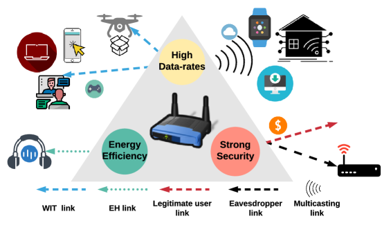
Figure 1: A system with multiple communication services.

To answer this question, it is enlightening to understand the current approaches to address those objectives. As an essential part of the multiple-input and multiple-output (MIMO) communication systems, precoding and power allocation schemes (or equivalently, transmit covariance matrix design) are typically used to address each of those facets independently of the others. More specifically, for each of the five objectives we mentioned (i.e., WIT, EH, SWIPT, PHY security, and multicasting), one or more independent solutions are developed in the literature (see in Table I). For some objective, such as WIT, an optimal closed-form solution is known, which is obtained via celebrated singular value decomposition (SVD) and water-filling [2]. Linear precoding and power allocation solutions for EH and SWIPT can be found in [3] and [4]. For others, such as PHY security in the MIMO wiretap channel, only sub-optimal or iterative solutions are known in general [5, 6, 7] as the problem is not convex. Among them, generalized singular value decomposition (GSVD)-based precoding [5] is fast, sub-optimal solution whereas alternating optimization with water-filling (AO-WF) [6] has better performance but requires much more time. Yet, those methods may not be close to the capacity in some antenna settings [8, 7]. Lastly, multicasting is a min-max fair problem to enlarge the transmission rate for all users. In the multiple-input single-output (MISO) case, semidefinite relaxation (SDR) techniques yield a closed-form solution [9]. In the MIMO case, a cyclic alternating ascent (CAA) linear precoding is proposed in [10].

TABLE I: The Desired Objectives and Existing Solutions

Configuration	Objective Function	Reference
$\mathcal{O}_{1}$	WIT	[2]
$\mathcal{O}_{2}$	EH	[3]
$\mathcal{O}_{3}$	SWIPT	[3, 4]
$\mathcal{O}_{4}$	PHY Security	[5, 6, 8, 7]
$\mathcal{O}_{5}$	Multicasting	[9, 10]

It is seen that various different approaches are used to design precoder for the problems listed in Table I and, yet, some of them are not effective in all antenna settings. Among those problems, $\mathcal{O}_{3}$ to $\mathcal{O}_{5}$ are more challenging. In the first part of this paper, we apply rotation-based precoding (RP) to the latter three problems. This approach uses one method of solution for all those three problems. More importantly, in general, it results in a better performance for these objectives when compared with existing methods. RP can be applied to all of those problems to unify the optimization approach. However, the optimization problems corresponding to those objectives are still solved individually.

In the second part of this paper, we introduce a unified deep neural network (DNN)-based precoder to solve optimization problem corresponding to all of those five objectives ($\mathcal{O}_{1}$ to $\mathcal{O}_{5}$) at once. This will settle the question we raised earlier in this paper. The new question is how we can “teach” a DNN [11] to concurrently and effectively “learn” all objectives together? To this end, we utilize a supervised DNN to learn from the solutions given by the RP by using the backpropagation algorithm which updates internal parameters from presentation layers [11]. We introduce an input feature to distinguish the objectives, and we interpret “learn” as the act of choosing the best precoder. DNN is a good “learner” due to its sensitivity to the same types of input and output pairs, even if mathematical models/solutions for those pairs are totally different. DNN-based precoding can realize unification by regulating all the input objectives with a same structure.

Before this work, DNN has separately been applied to many communications problems independently. To name a few, in [12], DNN is employed to model a Markov chain to obtain the rate-energy region of SWIPT in practical EH circuits. In [13], an autoencoder is proposed in which DNN learns the optimal mapping from encoder to decoder for PHY security. In [14], a DNN-based precoder for wiretap channel is considered for specific antenna settings. We do not expect that supervised DNN to significantly surpass conventional mathematical methods in communications; nevertheless, DNN holds promise for many front-end technologies in complex scenarios [15], such as spectrum intelligence which deceptively manages the radio resource [16, 17, 18]; transmission intelligence which focuses on reaching channel estimation and characterization [19, 20]; network intelligence which enhances the communication quality in a system-level [21].

I-A Motivation and Contribution

Apart from unifying precoder design for multi-objective systems discussed earlier, computation efficiency is another reason that motivates us to investigate a DNN-based precoder.

DNN is a universal function approximator [22] which has achieved a remarkable capacity of algorithm learning [23]. DNN is essentially a set of filters that is applied repeatedly to batches of the input. The network owns fixed times of convolution operation on weight matrices which can avoid the endless loop of iteration. In other words, DNN is able to achieve high resource utilization (e.g., matrix rather than vector operations on GPU), which in turn can substantially reduce the computation costs without sacrificing accuracy. As a data-driven technique, DNN is usually arranged offline and only needs to be performed once.

In this paper, we design a unified precoder based on a DNN architecture which explores a different way of thinking for wireless communication systems. Our main contributions are:

• We introduce rotation-based precoding and power allocation for multiple objectives, including WIT, EH, SWIPT, PHY security, and multicasting. To the best of our knowledge, there is no such work linking so many functions into one model. The rotation-based model can parameterize any covariance matrices, which makes it possible to train a DNN in a unified manner.

• Rotation-based precoders are designed for SWIPT, PHY security, and multicasting, and have a more stable and even better performance than existing methods. Higher secrecy rates are achieved over MIMO wiretap channels with different numbers of antennas. Besides, it enlarges the data transmission rates for multicasting with lower computational complexity.

• Then, we propose a unified DNN-based precoder which “learns” from the conventional mathematical models, including analytical solutions and RP. This precoding is able to solve all objectives at the same time, since the network is trained by all the functions together. To choose the objectives, we design an input feature utilizing binary code. The performance of the DNN-based precoding is very close to that of the conventional methods.

• The proposed DNN-based precoding is more efficient than the state-of-the-art iterative solutions. Specifically, it is more than an order of magnitude faster than numerical solutions using a central processing unit (CPU). In the scenario where a graphics processing unit (GPU) is affordable (like base stations), it takes an average execution time around $0.40$ms and $0.043$ms corresponding to 10 and 100 channels concurrently. These numbers are much smaller than the coherence time of the wireless channels.

• The performance of the DNN-based precoder is evaluated for different numbers of hidden layers (depth) and hidden nodes (width). Increasing the depth and width positively increases the performance but increases the computational complexity.

I-B Organizations and Notations

The remainder of this paper is organized as follows. We introduce the system models for the five objectives in Section II, and formulate rotation-based precoding in Section III. In Section IV, we propose the DNN architecture for our unified precoder. We illustrate the training process and results in Section V. Finally, we conclude the paper in Section VI.

Notations: Bold lowercase letters denote column vectors and bold uppercase letters denote matrices. ${a}_{i,j}$ represents the entry $(i,j)$ of matrix $\mathbf{A}$. ${\rm vec}(\cdot)$ vectorizes a matrix by cascading columns. $|\cdot|$, $(\cdot)^{T}$, ${\rm ln}(\cdot)$, ${\rm tr}(\cdot)$ are the absolute value, Euclidean norm, transpose, natural logarithm, respectively. ${\rm diag}(\cdot)$ designates the diagonal matrix of the set inside. ${\rm sign}(\cdot)$ extracts the sign of a real number. $E\{\cdot\}$ is the expectation of random variables. $[x]^{+}$ expresses the maximum value of 0 and $x$. $\mathbf{I}_{a}$ is an $a\times a$ identical matrix, and $\mathbf{0}_{a\times b}$ ($\mathbf{1}_{a\times b}$) is all-zeros (all-ones) matrix of dimension ${a\times b}$.

II System Models and Mathematical Preliminaries

II-A Channel Model

In this paper, we consider a MIMO wireless communication system with one transmitter and two receivers. The transmitter (Tx) is equipped with $m$ transmit antennas and broadcasts information to the users. Inside Tx, a linear precoder is applied as shown in Fig. 2. In this figure, $\mathbf{s}\triangleq[s_{1},\ldots,s_{m}]^{T}$ is an independent and unit power symbol vector, that is, $\mathbb{E}\{\mathbf{s}\mathbf{s}^{T}\}=\mathbf{I}_{m}$. $\mathbf{\Lambda}\triangleq{\rm diag}(\lambda_{1},\ldots,\lambda_{m})$ represents the power allocation matrix, and $\mathbf{V}\in\mathbb{R}^{m\times m}$ is the precoding matrix. Then, the transmitted signal $\mathbf{x}$ is

$$\mathbf{x}=\mathbf{V}\mathbf{\Lambda}^{\frac{1}{2}}\mathbf{s},$$ (1)

whose covariance matrix is $\mathbf{Q}\triangleq\mathbb{E}\{\mathbf{x}\mathbf{x}^{T}\}=\mathbf{V}\mathbf{\Lambda}\mathbf{V}^{T}$. The channel input is subject to an average total power constraint

$${\rm tr}(\mathbb{E}\{\mathbf{x}\mathbf{x}^{T}\})\leq P.$$ (2)

At the receivers’ side, user equipment 1 (UE1) and user equipment 2 (UE2) are equipped with $n_{1}$ and $n_{2}$ antennas, respectively. It is assumed that the transmission is over a flat fading channel. The input-output relations are given as

$$\mathbf{y}_{1}=\mathbf{H}_{1}\mathbf{x}+\mathbf{w}_{1},$$ (3a)

$$\mathbf{y}_{2}=\mathbf{H}_{2}\mathbf{x}+\mathbf{w}_{2},$$ (3b)

in which $\mathbf{y}_{1}\in\mathbb{R}^{n_{1}\times 1}$ and $\mathbf{y}_{2}\in\mathbb{R}^{n_{2}\times 1}$ are received signals at UE1 and UE2, ${\mathbf{H}_{1}}\in\mathbb{R}^{n_{1}\times m}$ and $\mathbf{H}_{2}\in\mathbb{R}^{n_{2}\times m}$ are the channels corresponding to UE1 and UE2, and $\mathbf{w}_{1}\in\mathbb{R}^{n_{1}\times 1}$ and $\mathbf{w}_{2}\in\mathbb{R}^{n_{2}\times 1}$ are independent and identically distributed (i.i.d) Gaussian noises with zero means and identity covariance matrices. The above-mentioned MIMO communication system can have multiple objectives as described in the following. Throughout this paper, $\mathcal{O}_{i}$ refers to objective $i$, $i\in\{1,\dots,5\}$, as described in Table I.

II-B Objectives

II-B1 WIT ($\mathcal{O}_{1}$)

In this objective, UE1 acts as an information decoding user who seeks for highest transmission rate over the MIMO channel, while UE2 is ignored. The information transmission capacity $\mathcal{C}_{1}$ is obtained by solving the following problem [2]

$$\textmd{(P1)}\quad\mathcal{C}_{1}\triangleq \max\limits_{\mathbf{Q}}\frac{1}{2}\log{|\mathbf{I}_{n_{1}}+\mathbf{H}_{1}\mathbf{Q}\mathbf{H}_{1}^{T}|},$$ (4a)

$${\;\;\rm s.t.\;}\mathbf{Q}\succeq\mathbf{0},\mathbf{Q}=\mathbf{Q}^{T},{\rm tr}(\mathbf{Q})\leq P.$$ (4b)

The optimal solution of (P1) is obtained using singular value decomposition (SVD) and water-filling algorithm [2]. The optimal covariance matrix in (P1) can be expressed as

$$\mathbf{Q}_{1}^{\ast}=\mathbf{A}\mathbf{B}\mathbf{A}^{T},$$ (5)

in which $\mathbf{A}$ is obtained as the right-singular vectors of the channel $\mathbf{H}_{1}$, and $\mathbf{B}$ in is obtained from water-filling algorithm [2]. Later, we will use this analytical solution to generate training sets for $\mathcal{O}_{1}$.

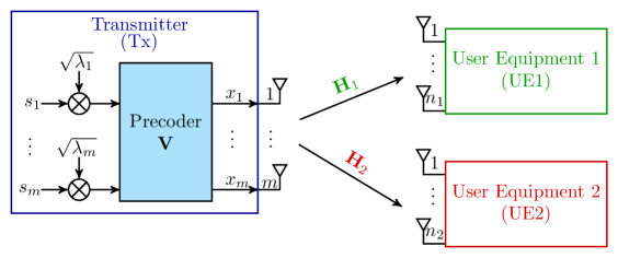
Figure 2: The two-user MIMO network with $m$, $n_{1}$, and $n_{2}$ antennas at Tx, UE1, and UE2, respectively. Here, $\mathbf{x}\in\mathbb{R}^{m\times 1}$ is the transmitted signal, $\mathbf{V}\in\mathbb{R}^{m\times m}$ is the precoding matrix, and $\lambda_{1},\ldots,\lambda_{m}$ are the powers allocated to symbols $s_{1},\ldots,s_{m}$, respectively.

II-B2 EH ($\mathcal{O}_{2}$)

EH refers to transmitting electrical energy originated from a power source. The transmitter emits radio-frequency signals, and UE2, as an EH user, tries to maximize the energy transmission efficiency. The objective function of this problem is shown in [3]

$$\textmd{(P2)}\quad\mathcal{C}_{2}\triangleq \max\limits_{\mathbf{Q}}\eta\cdot{\rm tr}(\mathbf{H}_{2}\mathbf{Q}\mathbf{H}_{2}^{T}),$$ (6a)

$${\;\;\rm s.t.\;}\mathbf{Q}\succeq\mathbf{0},\mathbf{Q}=\mathbf{Q}^{T},{\rm tr}(\mathbf{Q})\leq P,$$ (6b)

where $\eta$ is the converting rate of the harvested energy and, without loss of generality, we assume $\eta=1$ throughout the paper. The optimal analytical solution is given in [3]. It applies SVD to decompose channel $\mathbf{H}_{2}$ as $\mathbf{H}_{2}=\mathbf{E}\mathbf{F}\mathbf{G}^{T}$, in which $\mathbf{E}$ and $\mathbf{G}$ are orthonormal matrices and $\mathbf{F}$ is a diagonal matrix that contains non-negative singular values. If the diagonal elements of $\mathbf{F}$ are in descending order, then the optimal solution of (P2) is given as[3]

$$\mathbf{Q}_{2}^{\ast}=P\mathbf{g}_{1}\mathbf{g}_{1}^{T},$$ (7)

where $\mathbf{g}_{1}$ is the first column of $\mathbf{G}$.

II-B3 SWIPT ($\mathcal{O}_{3}$)

SWIPT is to balance the WIT from Tx to UE1 and the EH at UE2 simultaneously. As defined in [3], SWIPT characterizes the optimal trade-off between the maximum energy and information transfer by the rate-energy region which is formed as [3],

$$\textmd{(P3)}\quad\mathcal{C}_{3}\triangleq \max\limits_{\mathbf{Q}}\frac{1}{2}\cdot\log{|\mathbf{I}_{n_{1}}+\mathbf{H}_{1}\mathbf{Q}\mathbf{H}_{1}^{T}|},$$ (8a)

$${\;\;\rm s.t.\;}\ \eta\cdot{\rm tr}(\mathbf{H}_{2}\mathbf{Q}\mathbf{H}_{2}^{T})\geq{\cal\bar{E}},$$ (8b)

$$\;\qquad\mathbf{Q}\succeq\mathbf{0},\mathbf{Q}=\mathbf{Q}^{T},{\rm tr}(\mathbf{Q})\leq P,$$ (8c)

in which $\cal\bar{E}$ is a dynamic threshold representing the required minimum energy harvested by UE2. The value of $\cal\bar{E}$ is in the range from minimum (${\cal E}_{\min}$) to maximum (${\cal E}_{\max}$),

$${\cal{\bar{E}}}\triangleq{\cal E}_{\min}+q({\cal E}_{\max}-{\cal E}_{\min}),$$ (9)

where $q$ is called the normalized EH level and varies from $0\%$ to $100\%$. Since we are looking for the maximum rate-energy boundary, ${\cal E}_{\min}$ is defined as the energy received by UE2 when UE1 achieves the maximum data rate, i.e., (P1) reaches its optimal. Then, we have ${\cal E}_{\min}=\eta\cdot{\rm tr}(\mathbf{H}_{2}\mathbf{Q}_{1}^{\ast}\mathbf{H}_{2}^{T})$ where $\mathbf{Q}_{1}^{\ast}$ is given in (5). On the other hand, ${\cal E}_{\max}$ can be obtained when UE2 reaches the maximum EH level by solving (P2), i.e., ${\cal E}_{\max}=\mathcal{C}_{2}$. When $q=0\%$ or $q=100\%$, (P3) degenerates to (P1) and (P2), respectively.

II-B4 PHY Security ($\mathcal{O}_{4}$)

Under this objective, UE1 is a legitimate user and requires services while keeping it secret from an eavesdropper, UE2. The precoder is expected to maximize the secrecy transmission rate [24]

$$\textmd{(P4)}\quad\mathcal{C}_{4}\triangleq \max\limits_{\mathbf{Q}}\frac{1}{2}\log\frac{|\mathbf{I}_{n_{1}}+\mathbf{H}_{1}\mathbf{Q}\mathbf{H}_{1}^{T}|}{|\mathbf{I}_{n_{2}}+\mathbf{H}_{2}\mathbf{Q}\mathbf{H}_{2}^{T}|},$$ (10a)

$${\;\;\rm s.t.\;}\mathbf{Q}\succeq\mathbf{0},\mathbf{Q}=\mathbf{Q}^{T},{\rm tr}(\mathbf{Q})\leq P.$$ (10b)

An optimal analytical solution for MIMO wiretap channel only exist in limited cases, including the case when $n_{t}=2$ [8]. Other solutions are numerical like GSVD [5], AO-WF [6], etc.

II-B5 Multicasting ($\mathcal{O}_{5}$)

In this configuration, Tx offers a multicasting message to both users, such as advertisements and emergency alerts. To ensure the multicasting message can be decoded by everyone, multicasting rate is limited to the minimum rate of the receivers. The transmission rate of this problem is formulated as [10]

$$\textmd{(P5)}\quad\mathcal{C}_{5}\triangleq \max\limits_{\mathbf{Q}}\;\min\limits_{u=1,2}\frac{1}{2}\log{|\mathbf{I}_{n_{u}}+\mathbf{H}_{u}\mathbf{Q}\mathbf{H}_{u}^{T}|},$$ (11a)

$${\;\;\rm s.t.\;}\mathbf{Q}\succeq\mathbf{0},\mathbf{Q}=\mathbf{Q}^{T},{\rm tr}(\mathbf{Q})\leq P.$$ (11b)

In the MISO case, SDR techniques yield a closed-form solution [9]. In the MIMO case, CAA is proposed in [10], and [25] mentions that the problem can be solved by semidefinite programming (SDP) directly. Moreover, [26] introduced a nonlinear random search with rotation parameters. However, the existing methods are limited to the computational complexity or are only available for a specific number of antennas.

As we saw, (P1)-(P5) have different expressions and solutions in general. As the objective changes, the corresponding solution changes completely. Moreover, (P3)-(P5) can only be solved iteratively which incur high complexity and thus are slow. To tackle this, we first propose a unified solution for (P3)-(P5), which is robust and reliable in a variety of antenna settings. Then, we propose DNN-based precoding that can solve (P1)-(P5) simultaneously and efficiently.

III Rotation-based Precoding

In this section, we introduce RP and apply it to (P3)-(P5). We should highlight that RP can also be applied to (P1)-(P2) but these two problems have competitive analytical solutions, and there is no need to a new solution.

III-A Rotation-based Precoding (RP)

The covariance matrix $\mathbf{Q}$ can be formed using eigenvalue decomposition as

$$\mathbf{Q}\triangleq\mathbf{V}\mathbf{\Lambda}\mathbf{V}^{T},$$ (12)

in which $\mathbf{\Lambda}\in\mathbb{R}^{m\times m}$ is a diagonal matrix, whose diagonal elements $[\lambda_{1},\ldots,\lambda_{m}]$ are non-negative due to the PSD constraint. Then, the average power constraints in (P1)-(P5) are equivalent to $\sum_{i=1}^{m}\lambda_{i}\leq P$. Thus, the PSD and power constraints can be represented as a set of linear constraints

$$\{\lambda_{i}|\lambda_{i}\geq 0,\;\sum_{i=1}^{m}\lambda_{i}\leq P\}.$$ (13)

Besides, $\mathbf{V}\in\mathbb{R}^{m\times m}$ is an orthonormal matrix due to the symmetric property of $\mathbf{Q}$. It can be modeled as a Given’s matrix [27, 7] also named as a rotation matrix

$$\mathbf{V}=\prod_{i=1}^{m-1}\prod_{j=i+1}^{m}\mathbf{V}_{i,j},$$ (14)

where $\mathbf{V}_{i,j}$ is an identity matrix except for four elements

$$\left[\begin{matrix}v_{i,i}&v_{i,j}\\ v_{j,i}&v_{j,j}\end{matrix}\right]=\left[\begin{matrix}\cos\theta_{i,j}&-\sin\theta_{i,j}\\ \sin\theta_{i,j}&\cos\theta_{i,j}\end{matrix}\right].$$ (15)

Intuitively, for any vector $\mathbf{v}$ in $\mathbb{R}^{m\times 1}$ vector space, $\mathbf{V}_{i,j}\cdot\mathbf{v}$ represents a rotating from the $i$th standard basis to the $j$th standard basis with a certain rotation angle $\theta_{i,j}$. In total, we need

$$n_{a}=\frac{1}{2}m(m-1),$$ (16)

rotation angles to represent $\mathbf{V}$ in (14). There is no constraint on rotation angles, i.e., $\theta_{i,j}\in\mathbb{R}$. In [7], we have proved that an arbitrary covariance matrix $\mathbf{Q}$ can be represented by $m$ non-negative eigenvalues and $n_{a}$ rotation angles. Therefore, the optimization on $\mathbf{Q}$ can be equivalently transformed to optimization parameters using RP with the constraint (13).

It is worth mentioning that the order of multiplication in (14) is not unique and different order will lead to different rotation angles $\theta_{i,j}$. In this paper, without loss of generality, we use the order defined in (14). Then, the rotation parameter vector can be defined as

$$\mathbf{r}\triangleq[{\bm{\lambda}},{\bm{\theta}}]^{T},$$ (17)

where

$${\bm{\lambda}}\triangleq[\lambda_{1},\ldots,\lambda_{m}]\;\text{and}\;{\bm{\theta}}\triangleq[\theta_{1,2},\ldots,\theta_{m-1,m}].$$ (18)

To this end, $\mathbf{Q}$ can be specified by the parameter vector $\mathbf{r}$ with the new constraint

$$\mathbf{L}\mathbf{r}\leq\mathbf{b},$$ (19)

where

$$\textbf{}\mathbf{L}\triangleq\left[\begin{matrix}-\mathbf{I}_{m}&\mathbf{0}_{m\times n_{a}}\\ \mathbf{1}_{1\times m}&\mathbf{0}_{1\times n_{a}}\end{matrix}\right]\textrm{and}\;\mathbf{b}\triangleq\left[\begin{matrix}\mathbf{0}_{1\times m}\\ P\end{matrix}\right].$$ (20)

III-B Rotation-based Precoder for $\mathcal{O}_{3}$ to $\mathcal{O}_{5}$

The problems (P3)-(P5) are challenging and optimal analytical precoding matrices are not known. In the following, we apply RP to the problems, which can parameterize all of the problems with rotation angles and power allocation parameters.

III-B1 RP for SWIPT

Applying the RP on (P3), the objective function of SWIPT becomes

$$\textmd{(P3a)}\quad\mathcal{C}_{3}= \max\limits_{\mathbf{r}}\frac{1}{2}\log{|\mathbf{I}_{n_{1}}+\mathbf{H}_{1}\mathbf{Q}\mathbf{H}_{1}^{T}|},$$ (21a)

$${\;\;\rm s.t.\;}\mathbf{L}\mathbf{r}\leq\mathbf{b},$$ (21b)

$$\qquad\ \eta\cdot{\rm tr}(\mathbf{H}_{2}\mathbf{Q}\mathbf{H}_{2}^{T})\geq{\cal\bar{E}}.$$ (21c)

This problem can be solved by a general optimization tool such as fmincon in Matlab. Here, (21b) is a linear inequality constraint and (21c) can be added as non-linear constrain in fmincon. The For initialization of $\mathbf{Q}$ we use the solution of (P2), i.e., $\mathbf{Q}_{2}^{\ast}$ in (7). Then, we obtain the initial value $\mathbf{r}$ using (12)-(15) or Algorithm 1 in [7]. Finally, we can obtain $\mathbf{Q}_{3}^{\ast}$ which is defined to be the optimal solution for $\mathcal{O}_{3}$.

III-B2 RP for PHY Security

Applying RP to PHY Security problem results in

$$\textmd{(P4a)}\quad\mathcal{C}_{4}= \max\limits_{\mathbf{r}}\frac{1}{2}\log\frac{|\mathbf{I}_{n_{1}}+\mathbf{H}_{1}\mathbf{Q}\mathbf{H}_{1}^{T}|}{|\mathbf{I}_{n_{2}}+\mathbf{H}_{2}\mathbf{Q}\mathbf{H}_{2}^{T}|},$$ (22a)

$${\;\;\rm s.t.\;}\mathbf{L}\mathbf{r}\leq\mathbf{b}.$$ (22b)

Then, this new optimization problem can be solved by convex toolbox such as fmincon in Matlab. Then, we can obtain $\mathbf{Q}_{4}^{\ast}$ for $\mathcal{O}_{4}$. Although the PHY security is known as a non-convex problem, the performance of RP is more reliable compared with existing solutions, such as GSVD [5] and AO-WF [6].

III-B3 RP for Multicasting

Similarly, (P5) can be reformed as

$$\textmd{(P5a)}\quad\mathcal{C}_{5}= \max\limits_{\mathbf{r}}\;\min\left\{R_{u}\right\},u=1,2,$$ (23a)

$${\;\;\rm s.t.\;}\mathbf{L}\mathbf{r}\leq\mathbf{b},$$ (23b)

where $R_{u}$ represents the WIT rates of UE1 and UE2, i.e.,

$$R_{u}(\mathbf{Q})\triangleq\frac{1}{2}\log{|\mathbf{I}_{n_{u}}+\mathbf{H}_{u}\mathbf{Q}\mathbf{H}_{u}^{T}|},u=1,2.$$ (24a)

(P5a) is the minimum of two WIT problems represented in (P1) which is concave [2]. Thus, (P5a) is concave. Define the optimal solutions $\mathbf{Q}_{1}^{*(1)}$ and $\mathbf{Q}_{1}^{*(2)}$ for $R_{1}$ and $R_{2}$ in (24a). Then, the (P5a) in (23) can be solved by three sub-cases:

• Case 1: $R_{1}(\mathbf{Q}_{1}^{*(1)})\leq R_{2}(\mathbf{Q}_{1}^{*(1)})$, then the optimal multicast covariance matrix of (23) is $\mathbf{Q}^{*}_{5}=\mathbf{Q}_{1}^{*(1)}$.

• Case 2: $R_{1}(\mathbf{Q}_{1}^{*(2)})\geq R_{2}(\mathbf{Q}_{1}^{*(2)})$, the optimal multicast covariance matrix of (23) is $\mathbf{Q}^{*}_{5}=\mathbf{Q}_{1}^{*(2)}$.

• Case 3: Otherwise, we solve the rotation parameters in (23) using fmincon.

Since the first two sub-cases are actually WIT problems with analytical solutions, the efficiency of the solution improves compared to iterative solutions such as CAA [10] and SDP. Till now, the solutions $\mathbf{Q}^{*}_{3}$ to $\mathbf{Q}^{*}_{5}$ for $\mathcal{O}_{3}$ to $\mathcal{O}_{5}$ is obtained using the RP, respectively. In the next section, we propose using supervised DNN to learns from the above solutions and find the covariance matrices corresponding to (P1)-(P5) at once.

IV A Unified DNN-based Precoder

In this section, we introduce a unified DNN-based precoding and power allocation, including the DNN structure, the input features, and network outputs. DNN can increase the efficiency by unifying the solution for all of the problems together in contrast to the conventional methods which perform optimization one by one.

Before talking about the details of the DNN, we indicate that $\mathcal{O}_{3}$ (the SWIPT problem) will be differentiated for nine normalized EH level in (9) for

$$q\in\{90\%,80\%,\ldots,10\%\}.$$ (25)

These sub-problems are named $\mathcal{O}_{3}$(90$\%$) to $\mathcal{O}_{3}$(10$\%$) as shown in Table II. Then, for the proposed DNN, a unique index $\mathcal{M}_{k}$, $k\in\{1,\ldots,K\}$, represents different modes. Therefore, we have $K=13$ modes in total. It is worth clarifying that $\mathcal{O}_{i}$ refers to the configurations of precoding objectives, i.e., WIT, EH, etc., while we use $\mathcal{M}_{k}$ for integer index and simplifying the expressions. These are listed in Table II for clarity.

IV-A The DNN Structure

The structure of the proposed DNN-based precoding is demonstrated in Fig. 3. At the top, the parameters of the two users, including mode and channel selection. The DNN-based precoder can provide the precoding solution directly, while it is necessary to activate one of the conventional methods according to the user requirement. The DNN-based precoder can be divided into three parts shown by different colors in Fig. 3. These are 1) the input layer, which pre-processes the input information and generates a feature vector for DNN; 2) DNN is applied to achieve the non-linear mapping between the features and demanded outputs; 3) the output layer that maps the output to a covariance matrix for precoding.

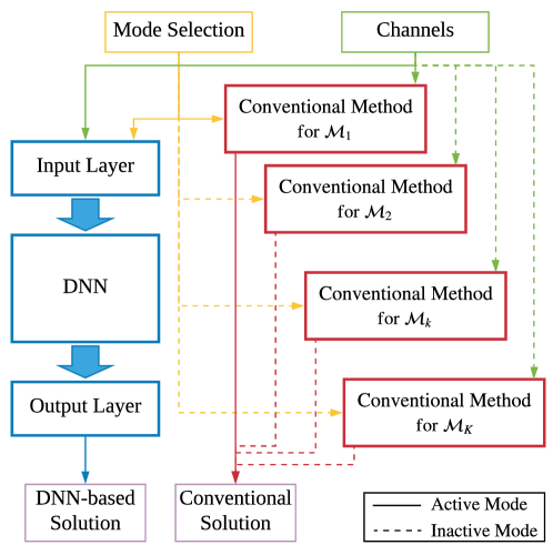
Figure 3: The structure of the proposed DNN-based precoding. The current selected mode is $\mathcal{M}_{k}$.

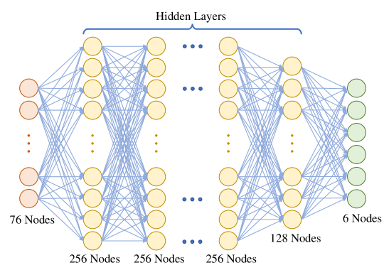
Figure 4: The DNN architecture.

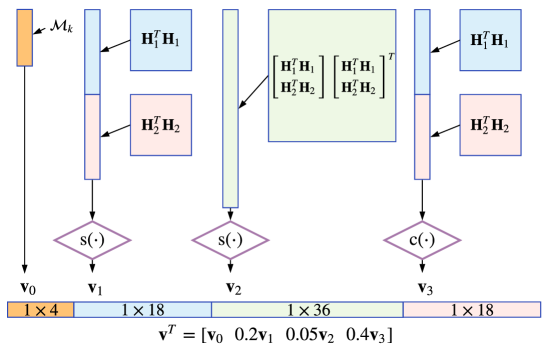
Figure 5: Feature design for the input layer.

As shown in Fig. 4, the architecture of the DNN precoder has ten fully-connected hidden layers equipped with parametric rectified linear units (PReLU) [28] as activation functions. PReLU is defined as

$$f(y)=\left\{\begin{matrix}y,&y\geq 0,\\ \alpha y,&y<0,\\ \end{matrix}\right.$$ (26)

where $\alpha=0.25$ is a trainable initialized parameter. PReLU extends the freedom of the DNN to mimic a mapping and preventing over-fitting at the same time.

IV-B Input Features

TABLE II: Code Vector Design for Each Mode

Objective	Mode	Code ($\mathbf{c}_{k}$)	Objective	Mode	Code ($\mathbf{c}_{k}$)
$\mathcal{O}_{1}$	$\mathcal{M}_{1}$	0001	$\mathcal{O}_{3}$$(40\%)$	$\mathcal{M}_{8}$	1000
$\mathcal{O}_{2}$	$\mathcal{M}_{2}$	0010	$\mathcal{O}_{3}$$(30\%)$	$\mathcal{M}_{9}$	1001
$\mathcal{O}_{3}$$(90\%)$	$\mathcal{M}_{3}$	0011	$\mathcal{O}_{3}$$(20\%)$	$\mathcal{M}_{10}$	1010
$\mathcal{O}_{3}$$(80\%)$	$\mathcal{M}_{4}$	0100	$\mathcal{O}_{3}$$(10\%)$	$\mathcal{M}_{11}$	1011
$\mathcal{O}_{3}$$(70\%)$	$\mathcal{M}_{5}$	0101	$\mathcal{O}_{4}$	$\mathcal{M}_{12}$	1100
$\mathcal{O}_{3}$$(60\%)$	$\mathcal{M}_{6}$	0110	$\mathcal{O}_{5}$	$\mathcal{M}_{13}$	1101
$\mathcal{O}_{3}$$(50\%)$	$\mathcal{M}_{7}$	0111

The schematic diagram of the input layer is shown in Fig. 5. The required inputs are $\mathbf{H}_{1}$, $\mathbf{H}_{2}$, and mode index, which given by $k\in\{1,\ldots,K\}$. The feature vector contains four sub-features, namely, $\mathbf{v}_{0}$, $\mathbf{v}_{1}$, $\mathbf{v}_{2}$, and $\mathbf{v}_{3}$ which are

$$\mathbf{v}_{0}\triangleq\mathbf{c}_{k},$$ (27a)

$$\mathbf{v}_{1}\triangleq{\rm s}({\rm vec}(\mathbf{F}))^{T},$$ (27b)

$$\mathbf{v}_{2}\triangleq{\rm s}({\rm vec}(\mathbf{F}^{T}\mathbf{F}))^{T},$$ (27c)

$$\mathbf{v}_{3}\triangleq{\rm c}({\rm vec}(\mathbf{F}))^{T},$$ (27d)

where $\mathbf{c}_{k}\in\mathbb{R}^{1\times 4}$ is a binary-code vector identifying the $k$-th objective. The objectives and the corresponding code are listed in Table II. $\mathbf{F}$ contains channel information defined as

$$\mathbf{F}\triangleq[\mathbf{H}_{1}^{T}\mathbf{H}_{1}\;\;\mathbf{H}_{2}^{T}\mathbf{H}_{2}].$$ (28)

${{\rm s}(x)}$ is the element-wise square root function keeping the sign of input $x$, i.e.,

$${\rm s}(x)\triangleq{\rm sign}(x)\cdot|x|^{\frac{1}{2}},$$ (29)

Similarly, ${\rm c}(x)$ is the element-wise cubic root function, which defined as

$${\rm c}(x)\triangleq{\rm sign}(x)\cdot|x|^{\frac{1}{3}}.$$ (30)

Among the sub-feature vectors, $\mathbf{v}_{0}$ represents the feature with respect to the mode index. With such a definition, the DNN has a better performance in recognizing the input objectives. Besides, $\mathbf{v}_{1}$, $\mathbf{v}_{2}$, and $\mathbf{v}_{3}$ are formed based on channels matrices. We use $\mathbf{H}_{1}^{T}\mathbf{H}_{1}$ and $\mathbf{H}_{2}^{T}\mathbf{H}_{2}$ rather than using $\mathbf{H}_{1}$ and $\mathbf{H}_{2}$ directly, since

$$|\mathbf{I}+\mathbf{H}\mathbf{Q}\mathbf{H}|=|\mathbf{I}+\mathbf{H}^{T}\mathbf{H}\mathbf{Q}|,$$ (31a)

$${\rm tr}(\mathbf{H}\mathbf{Q}\mathbf{H}^{T})={\rm tr}(\mathbf{H}^{T}\mathbf{H}\mathbf{Q}),$$ (31b)

can be applied to optimization problems introduced in Section II. With such a definition, the dimension of input features is related only to $m$ rather than $m$, $n_{1}$, and $n_{2}$. Furthermore, non-linear combinations of channels are also considered to deliver more information to the DNN in order to achieve a better non-linear capability.

Considering that the distribution of the channel elements are Gaussian, the elements of $\mathbf{F}$ have a high density concentrating around $0$. This decreases the fairness and distinguishability of the input features. To overcome this problem, we use square root and cubic root in (27b)-(27d) to flattens the distribution of the features to some degree. Finally, the input feature vector $\mathbf{v}$ is a cascade of these sub-feature vectors

$$\mathbf{v}\triangleq[\mathbf{v}_{0},0.2\mathbf{v}_{1},0.05\mathbf{v}_{2},0.4\mathbf{v}_{3}]^{T},$$ (32)

where the coefficients are chosen experimentally to normalize the sub-feature vectors and improve the accuracy of the DNN and the speed of learning [29, 30]. In this paper, we consider $P=20$ and $m=3$ while $n_{1}$ and $n_{2}$ can be any number based on specific cases. In this scenario, the size of the input of the DNN is $76$ .

IV-C Network Outputs

Since the covariance matrix is symmetric, the output (vector $\mathbf{q}$) contains only upper triangular elements of $\mathbf{Q}$. That is,

$$\mathbf{q}\triangleq[q_{1,1},q_{2,2},q_{3,3},q_{1,2},q_{2,3},q_{1,3}]^{T}.$$ (33)

Then, $\mathbf{Q}$ can be assembled as

$$\mathbf{Q}=\left[\begin{matrix}q_{1,1}&q_{1,2}&q_{1,3}\\ q_{2,1}&q_{2,2}&q_{2,3}\\ q_{3,1}&q_{3,2}&q_{3,3}\end{matrix}\right]=\mathbf{V}\mathbf{\Lambda}\mathbf{V}^{T}.$$ (34)

The precoding and power allocation matrices $\mathbf{V}$ and $\mathbf{\Lambda}$, respectively, are obtained by eigenvalue decomposition. To ensure the PSD and total power constraints, negative diagonal elements in $\mathbf{\Lambda}$ are normalized to zero and the trace is scaled to $P$. In the training procedure, $\mathbf{q}$ is known through RP corresponding to the problem discussed in Section III. Whereas, during testing, $\mathbf{Q}$ will be obtained from the output vector and the precoding solution is obtained by eigenvalue decomposition [14].

V Training procedure and Numerical Results

In this section, we initially verify the performance of RP which is used to train the network. Then, we explain the details of our data set and the training procedure. Finally, we examine the performance of the proposed DNN-based precoding.

V-A Performance of RP

V-A1 SWIPT ($\mathcal{O}_{3}$)

In Fig. 6, the performance of RP is compared with the time-switching and power-splitting (TS-PS) [3] and random trials of $\mathbf{Q}$. For RP and TS-PS, eleven thresholds ${\cal{\bar{E}}}$ equally dividing the interval $[{\cal E}_{\min},{\cal E}_{\max}]$ are considered in the cases of $P=10$, $20$, and $40$ (W). The channels matrices, which were generated randomly, are

$$\mathbf{H}_{1}=\left[\begin{matrix}-2.2975&0.4896&-1.8310\\ 1.4576&-0.6100&0.3800\\ 0.8998&0.0916&-0.3128\end{matrix}\right],$$ (35a)

$$\mathbf{H}_{2}=\left[\begin{matrix}-0.3276&3.3159&-0.9956\\ 1.5765&0.2604&0.2578\\ -0.3337&1.1478&-0.3364\end{matrix}\right].$$ (35b)

For both channels, RP can reach the same rate-energy region as TS-PS. The random trials are based on $10,000$ realizations of $\mathbf{Q}$.

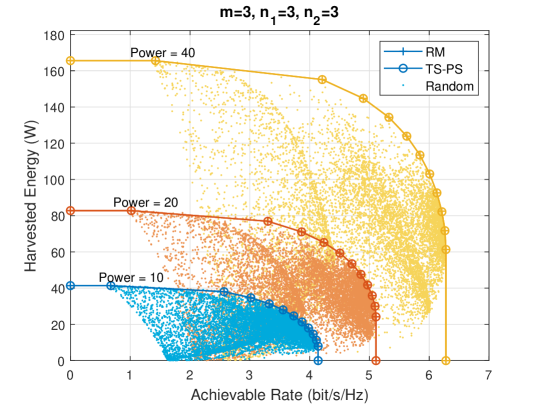
Figure 6: Comparisons of SWIPT region for the RP and TS-PS for 10,000 random trials. The colors distinguish different transmit powers.

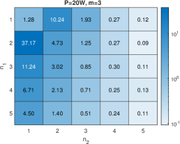
(a) Relative improvement ($\%$) of RP to GSVD.

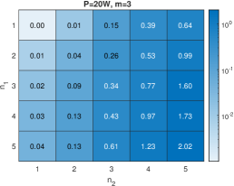
(b) Relative improvement ($\%$) of RP to AO-WF.

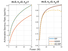
(c) Typical cases that RP exceed GSVD or AO-WF.

Figure 7: Comparisons between the secrecy transmission rate of the RP with GSVD and AO-WF.

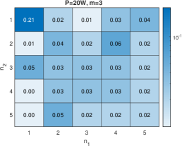
(a) Relative improvement ($\%$) of RP to CAA.

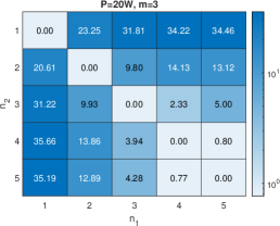
(b) Relative improvement ($\%$) of RP to SDP.

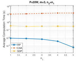
(c) The time consumption of each method.

Figure 8: Comparisons between the multicasting transmission rate and computational cost of the RP with CAA and SDP.

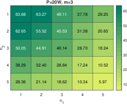
Figure 9: The probability ($\%$) that Case-3 occurswhen the RP is used for multicasting problem.

V-A2 PHY security ($\mathcal{O}_{4}$)

In this subsection, we consider the MIMO wiretap channel. The performance of RP is compared with GSVD [5] and AO-WF [6] in Fig. 7. The achievable secrecy rates are averaged over 200 random channel realizations, where the channels are generated as independent standard Gaussian random variables. Fig. 7(a) and Fig. 7(b) represent relative improvement defined as

$$\eta_{g}=\frac{(R_{r}-R_{g})}{R_{g}}\times 100\%,$$ (36a)

$$\eta_{a}=\frac{(R_{r}-R_{g})}{R_{g}}\times 100\%,$$ (36b)

in which $\eta_{g}$ and $\eta_{a}$ represent the percentages that RP exceeds GSVD and AO-WF, i.e., the bluer, the better. $R_{r}$, $R_{g}$, and $R_{a}$ are the average secrecy rate achieved by RP, GSVD, and AO-WF, respectively. $P=20$W and $m=3$ are set in this figure. Each cell denotes a pair of $n_{1}$ and $n_{2}$. The proposed RP is able to achieve a better secrecy rate in any antenna setting. There is a noticeable gap between RP and GSVD when the eavesdropper has a smaller number of antennas. For a larger $n_{2}$, RP is capable of reaching a higher secrecy rate compared to AO-WF. Further illustrations are shown in Fig. 7(c) considering two cases over 200 channel realizations. The plots show the average secrecy rates versus transmit power in the case of $m=3$, $n_{1}=2$, $n_{2}=1$ and $m=3$, $n_{1}=3$, $n_{2}=5$. We see that RP can perform stably and reliably in those cases. Moreover, the average time costs over all cases in Fig. 7(b) of RP is $27.65$ms which is less than $38.26$ms achieved by AO-WF.

V-A3 Multicasting ($\mathcal{O}_{5}$)

For multicasting, we compare RP with the CAA [10] and standard SDP techniques. Here, we apply CVX [31] to realize SDP solutions for multicasting.

We investigate a variety of combinations of $\{n_{1},n_{2}\}$, and the results are listed in Fig. 8. Similar to (36a)-(36b), we define the relative improvement factors $\eta_{c}$ and $\eta_{s}$ representing the percentages that RP exceeds CAA and SDP, respectively. It can be seen from Fig. 8(a) that RP slightly beats CAA. Besides, RP outperforms SDP when $n_{1}\neq n_{2}$. This advantage is especially remarkable when $n_{1}>n_{2}=1$ or $n_{2}>n_{1}=1$ in Fig. 8(b). It is worth noting that, in the case of $n_{1}=n_{2}$, RP has a very close performance to SDP. This can be found in the diagonal of Fig. 8(b).

Moreover, the benefits of RP in reducing complexity cannot be ignored, which is analyzed in Fig. 8(c). Fig. 8(c) compares the time cost when $n_{1}=n_{2}$ where SDP works well. It can be seen that RP has the best efficiency, while CAA is computationally expensive due to the successive optimization SDP problem. The improvement of time efficiency is partially due to the sub-cases we divided in Section III-B3. In Case-1 and Case-2, the solution can be obtained analytically, which is much efficient than Case-3. The probability of Case-3 is estimated by the Monte Carlo method. The results are obtained over $20,000$ random channels for each specific $n_{1}$ and $n_{2}$ with fixed $P=20$W and $m=3$. As shown in Fig. 9, the probability of Case-3 is reduced with the increase of $n_{1}$ and $n_{2}$, which explains the drop in the time cost of RP in Fig. 8(c).

In summary, RP provides a unified solution for the studied precoding problems. It is feasible for SWIPT. Also, it is reliable for PHY security and multicasting problems in the variety of the number of transmit and receive antennas.

V-B Data Set Generation and Training Procedure

In order to evaluate the performance of the proposed DNN-based precoding, we generate over two million random realizations of $\mathbf{H}_{1}$ and $\mathbf{H}_{2}$. Each element of the channels follows $\mathcal{N}(0,1)$. From these channel realizations, $2,000,000$ channels contribute to the training set and $10,000$ of them are used for testing. Since the number of transmit antennas $m$ and power $P$ are fixed at the Tx side, we set $m=3$ and $P=20$W in all training and test sets. The number of antennas of UE1 and UE2, i.e., $n_{1}$ and $n_{2}$, are randomly chosen from $1$ to $5$ covering most cases of user devices.

For each channel realization in the training and test sets, we generate $13$ samples (defined as input-output pairs) corresponding to the $K$ objectives in Table II. In such $K$ samples, each one contains an input feature vector according to (32) and a corresponding output vector $\mathbf{q}$ formulated as (33) given by the solution of the RP method. That is, for $\mathcal{O}_{1}$ and $\mathcal{O}_{2}$, we have analytical solutions given in Section II-B1 and II-B2; while for $\mathcal{M}_{3}$ to $\mathcal{M}_{5}$, the RP method for each is given in Section III-B1 to III-B3. Therefore, the training set has $26,000,000$ samples and the test set has $130,000$ samples. The details of training and test sets are summarized in Table III.

TABLE III: Data Sets Generation.

Stage	$m$	$n_{1}$	$n_{2}$	Number of Channels	Number of Samples
Training	3	$1,\ldots,5$	$1,\ldots,5$	2,000,000	26,000,000
Test	3	$1,\ldots,5$	$1,\ldots,5$	10,000	130,000

The training procedure is executed on a single graphical card (NVIDA GeForce GTX 1660Ti) using Adam[32] as an optimization method. All training procedures share the same group of hyper-parameters as listed in Table IV. The learning rate controls how quickly the DNN can change the weights, and it drops by $20\%$ after one epoch in this paper. Mini batch size indicates how many samples are considered together for one update of the DNN weights. Max epochs denotes the times that all data set has been taken into the training procedure. After the training process, the DNN-based precoding is ready for testing.

TABLE IV: Hyper-parameters in Training Procedure.

Hyper-parameter	Value	Hyper-parameter	Value
Initial learning rate	0.001	Mini batch size	5000
Learn rate drop factor	0.8	Max epochs	50
Learn rate drop period	1

V-C Numerical Results

In this part, we evaluate the performance of the proposed unified DNN-based precoding in different antenna settings. The DNN precoder is used in the following way. Two users are equipped with any number of antennas covering from $1$ to $5$, respectively. For a given channel pairs $\mathbf{H}_{1}$ and $\mathbf{H}_{2}$ with a required mode from Table II, the input layer converts the channels and the mode to sub-feature vectors as (27b)-(27d) and (27a), respectively. Then, the output $\mathbf{q}$ in (33) can be found in the output layer.

The evaluation of the DNN-precoder contains three metrics:

1. The mean square error (MSE) of elements in $\mathbf{Q}$ provided by the DNN-based precoding;

2. The performance compared to the conventional methods.

3. Time consumption for each objective.

V-C1 MSE of elements of $\mathbf{Q}$

The MSE is evaluated to ensure the feasibility. The MSE is defined as the variance between the ${q}_{i,j}$ given by DNN-based precoder and the one obtained by the corresponding conventional method. The MSE is between $0.0652$ and $0.0918$ averaged over $130,000$ samples in the test set, which indicates the capability of DNN-based precoding.

V-C2 Performance evaluation

The performance of the proposed DNN-based precoder for each objective is shown in Fig. 10, where the achievable rate is in bit/s/Hz and harvested energy in Watt is normalized by the baseband symbol period [3]. Here we plot the first fifty channel realizations from the test set for each objective. We choose $\mathcal{O}_{3}$($60\%$) and $\mathcal{O}_{3}$($20\%$) as representatives for SWIPT. In each subfigure, the solid line represents the achievable rate or harvested energy obtained by conventional methods (analytical solutions for $\mathcal{O}_{1}$ and $\mathcal{O}_{2}$, and RP for $\mathcal{O}_{3}$ to $\mathcal{O}_{5}$), whereas the dashed light-colored line is the result given by the DNN-precoder. It can be seen that the results are almost fitting the corresponding conventional solutions.

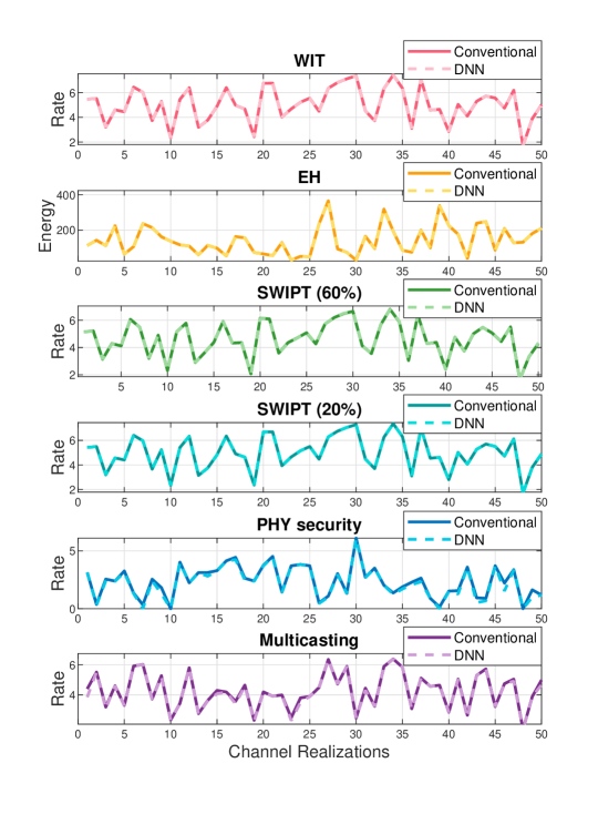
Figure 10: The performance of the proposed DNN-based precoder compared with conventional methods on 6 objectives. In this figure, the achievable rate is in bit per second per hertz (bit/s/Hz) and harvested energy is in Watt (W).

The average achievable rates or harvested energy are reported in Table V. The accuracy is defined as the percentage of DNN-precoder to the conventional methods, i.e.,

$$\zeta_{d}^{(k)}\triangleq\frac{R_{d}^{(k)}}{R_{c}^{(k)}}\times 100\%,\qquad k\in\{1,\ldots,13\},$$ (37)

where $k$ is the mode index, $R_{d}^{(k)}$ and $R_{c}^{(k)}$ are the results (achievable rate or harvested energy) of DNN-precoder and the conventional method. Average accuracy is listed in Table V. On average, the accuracy is $99.45\%$ among all tasks. The performance of the DNN-precoder could be seen the same as the RP method except for $\mathcal{O}_{4}$.

TABLE V: Average Achievable Rate (bit/s/Hz) or Harvested Energy (W).

Objective	Conventional	DNN	Accuracy ($\%$)
$\mathcal{O}_{1}$	4.9746	4.9733	99.97
$\mathcal{O}_{2}$	132.48	132.26	99.84
$\mathcal{O}_{3}$($60\%$)	4.5637	4.5625	99.96
$\mathcal{O}_{3}$($20\%$)	4.9279	4.9261	99.97
$\mathcal{O}_{4}$	2.3153	2.1809	94.19
$\mathcal{O}_{5}$	4.0142	3.9798	99.14

It is worth mentioning that the work in [14] is specifically aimed at $\mathcal{O}_{4}$ and is only feasible for $\{n_{1}=4,n_{2}=3\}$ and $\{n_{1}=2,n_{2}=1\}$. The accuracy in [14] is 97.71$\%$ and 93.72$\%$. In this paper, the DNN-precoder is able to achieve 96.94$\%$ and 93.15$\%$ on those two settings of $n_{1}$ and $n_{2}$. The slight loss is attributed to much wider antenna settings in this problem as shown in Table III.

Next, the rate-energy region of SWIPT is demonstrated with more details. We have arranged nine modes for SWIPT inside the DNN-based precoding, which can be generated as an achievable rate-energy region for any arbitrary channel. In Fig.11, DNN-based solution is compared with conventional methods using the channels in (35). Both of the methods have been executed for $q=[100\%,90\%,\ldots,0\%]$. For the DNN-based precoding, $q=100\%$ is actually $\mathcal{O}_{2}$, EH; $q=0\%$ is obtained by $\mathcal{O}_{1}$, the WIT. Those two methods provide almost the same rate-energy region.

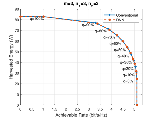
Figure 11: The rate-energy region achievable by DNN-precoder for SWIPT.

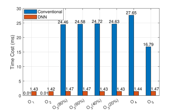
Figure 12: The time cost of each objectives.

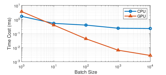
Figure 13: Average execution time over different batch sizes.

V-C3 Time consumption

The average time consumption (averaged over 10,000 channels) of the conventional and DNN-based solutions is compared with conventional methods in Fig. 12. All objectives are implemented on the same CPU, channel by channel. For $\mathcal{O}_{1}$ and $\mathcal{O}_{2}$, conventional methods are more efficient since they are analytical solutions and are faster than the DNN-based precoder. The advantage of the DNN-based precoder will appear on other objectives where only numerical solutions exist. The conventional methods require around 16ms to 27ms to achieve solutions while the proposed DNN-based precoding needs less than 1.5ms. On average, it saves $91.91\%$ of run-time if we assume that the four objectives occur with the same probability.

This indicates that the proposed method is promising for IoT applications as IoT devices which have limited computation capabilities and battery lifetime. DNN-based precoding is also good for complicated equipment, such as base stations that serve a large number of users at the same time, where GPUs are affordable for more than one channel. The average time will reduce dramatically attributed to the parallel computing ability of GPU. We use the batch size denoting the number of channels or objectives processed simultaneously. Fig. 13 reveals the relation between batch size and time computation using CPU and GPU. For example, when batch size is 100, the time cost is 0.4007ms on CPU and 0.0426ms on GPU. Then, the computational load can be largely reduced.

We understand that generating data sets and training the network is time-consuming. However, these procedures are performed only once and in an offline manner. Once this is done, the DNN-based precoder becomes a matrix multiplication that can be used as long as the assumption on the channels are valid. On the other hand, for the conventional solution the optimization problem corresponding to each objective need to be solved for each input channel independently. So, the DNN approach shows its advantages in long-term usages.

TABLE VI: The Accuracy ($\%$) and Time Consumption (ms) of the DNN-based Precoding with Different Depths and Widths

. Width Depth Objective Time Cost $\mathcal{O}_{1}$ $\mathcal{O}_{2}$ $\mathcal{O}_{3}$($80\%$) $\mathcal{O}_{3}$($60\%$) $\mathcal{O}_{3}$($40\%$) $\mathcal{O}_{3}$($20\%$) $\mathcal{O}_{4}$ $\mathcal{O}_{5}$ (ms) 128 10 99.91 99.52 99.87 99.94 99.90 99.91 89.65 98.62 0.94 256 6 99.92 99.58 99.79 99.93 99.94 99.90 90.69 98.69 1.39 256 10 99.97 99.84 99.95 99.97 99.97 99.96 94.19 99.14 1.44 256 14 99.98 99.91 99.95 99.98 99.99 99.97 96.75 99.15 2.03 512 10 99.98 99.90 99.97 99.98 99.98 99.98 96.41 99.46 2.39

V-D The Scale of DNN-based Precoding

In this part, we evaluate the performance of the DNN-based precoding associate with the depth (number of hidden layers) and the width (number of hidden nodes) of the network. The proposed DNN has ten layers in which nine of them have $256$ hidden nodes and the last one has $128$ hidden nodes. So we define this network as 10 in depth and 256 in width. Other networks are trained and tested in the same way as we have done in the previous experiments. The performance is listed in Table VI, including the accuracy in (37) and average time cost. For $\mathcal{O}_{1}$ and $\mathcal{O}_{3}$, all of the networks work well and close to the RP. The performance and the time cost of $\mathcal{O}_{2}$, $\mathcal{O}_{4}$, and $\mathcal{O}_{5}$ are positively related to depth and width. As a balance of solution quality and time consumption, we choose the depth as 10 and width as 256 in this paper, even though better performance can be achieved using a deeper and wider network.

VI Conclusion

In this paper, a unified DNN-based precoder has been proposed for green, secure wireless transmission in two-user MIMO systems. Specifically, WIT, EH, SWIPT, PHY security, and multicasting problems have been considered. We first use rotation-based precoding to derive the transmit covariance matrix for the above problems from which the DNN learns. The overall performance of the rotation-based precoder is better than the existing methods for SWIPT, PHY security, and multicasting. These conventional methods based on the mathematical models are used for data set generation and training procedure of DNN. Next, a DNN-based precoder is designed to unify the solutions for different objectives. This DNN-based precoding can effectively optimize all objectives at the same time. In terms of achievable rates and harvested energy, The performance of the unified DNN-based precoder is similar to the method it learns from, whereas its time cost is substantially lower than the conventional iterative solutions. Due to its lower computational complexity and its high flexibility, the proposed precoding is suitable for emerging existing applications, where the low-latency and low-complexity devices are necessary.

References

- [1] Statista, “COVID-19 impact on digital communications in the U.S. 2020,” 2020. https://www.statista.com/topics/6241/coronavirus-impact-on-online-usage-in-the-us.
- [2] T. M. Cover and J. A. Thomas, Elements of Information Theory. John Wiley & Sons, 2012.
- [3] R. Zhang and C. K. Ho, “MIMO broadcasting for simultaneous wireless information and power transfer,” IEEE Transactions on Wireless Communications, vol. 12, no. 5, pp. 1989–2001, 2013.
- [4] J. Rostampoor, S. M. Razavizadeh, and I. Lee, “Energy efficient precoding design for SWIPT in MIMO two-way relay networks,” IEEE Transactions on Vehicular Technology, vol. 66, no. 9, pp. 7888–7896, 2017.
- [5] S. A. A. Fakoorian and A. L. Swindlehurst, “Optimal power allocation for GSVD-based beamforming in the MIMO Gaussian wiretap channel,” in Proc. IEEE International Symposium on Information Theory (ISIT), pp. 2321–2325, 2012.
- [6] Q. Li, M. Hong, H.-T. Wai, Y.-F. Liu, W.-K. Ma, and Z.-Q. Luo, “Transmit solutions for MIMO wiretap channels using alternating optimization,” IEEE Journal on Selected Areas in Communications, vol. 31, no. 9, pp. 1714–1727, 2013.
- [7] X. Zhang, Y. Qi, and M. Vaezi, “A rotation-based method for precoding in Gaussian MIMOME channels,” arXiv preprint arXiv:1908.00994, 2019.
- [8] M. Vaezi, W. Shin, and H. V. Poor, “Optimal beamforming for Gaussian MIMO wiretap channels with two transmit antennas,” IEEE Transactions on Wireless Communications, vol. 16, no. 10, pp. 6726–6735, 2017.
- [9] N. D. Sidiropoulos, T. N. Davidson, and Z.-Q. Luo, “Transmit beamforming for physical-layer multicasting,” IEEE Transactions on Signal Processing, vol. 54, no. 6, pp. 2239–2251, 2006.
- [10] H. Zhu, N. Prasad, and S. Rangarajan, “Precoder design for physical layer multicasting,” IEEE Transactions on Signal Processing, vol. 60, no. 11, pp. 5932–5947, 2012.
- [11] Y. LeCun, Y. Bengio, and G. Hinton, “Deep learning,” Nature, vol. 521, no. 7553, p. 436, 2015.
- [12] N. Shanin, L. Cottatellucci, and R. Schober, “Rate-power region of SWIPT systems employing nonlinear energy harvester circuits with memory,” arXiv preprint arXiv:1911.01115, 2019.
- [13] R. Fritschek, R. F. Schaefer, and G. Wunder, “Deep learning for the Gaussian wiretap channel,” in Proc. IEEE International Conference on Communications (ICC), pp. 1–6, 2019.
- [14] X. Zhang and M. Vaezi, “Deep learning based precoding for the MIMO Gaussian wiretap channel,” in Proc. IEEE Global Communications Conference (GLOBECOM) Workshops, 2019.
- [15] F.-L. Luo, Machine Learning for Future Wireless Communications. Wiley-Blackwell, 2019.
- [16] W. Lee, “Resource allocation for multi-channel underlay cognitive radio network based on deep neural network,” IEEE Communications Letters, vol. 22, no. 9, pp. 1942–1945, 2018.
- [17] K. N. Doan, M. Vaezi, W. Shin, H. V. Poor, H. Shin, and T. Q. Quek, “Power allocation in cache-aided noma systems: Optimization and deep reinforcement learning approaches,” IEEE Transactions on Communications, 2019.
- [18] S. D’Oro, A. Zappone, S. Palazzo, and M. Lops, “A learning approach for low-complexity optimization of energy efficiency in multicarrier wireless networks,” IEEE Transactions on Wireless Communications, vol. 17, no. 5, pp. 3226–3241, 2018.
- [19] T. O’Shea and J. Hoydis, “An introduction to deep learning for the physical layer,” IEEE Transactions on Cognitive Communications and Networking, vol. 3, no. 4, pp. 563–575, 2017.
- [20] X. Li and A. Alkhateeb, “Deep learning for direct hybrid precoding in millimeter wave massive MIMO systems,” arXiv preprint arXiv:1905.13212, 2019.
- [21] S. Fan, H. Tian, and C. Sengul, “Self-optimization of coverage and capacity based on a fuzzy neural network with cooperative reinforcement learning,” EURASIP Journal on Wireless Communications and Networking, vol. 2014, no. 1, p. 57, 2014.
- [22] K. Hornik, M. Stinchcombe, and H. White, “Multilayer feedforward networks are universal approximators.,” Neural Networks, vol. 2, no. 5, pp. 359–366, 1989.
- [23] B. Zoph and Q. V. Le, “Neural architecture search with reinforcement learning,” arXiv preprint arXiv:1611.01578, 2016.
- [24] T. Liu and S. Shamai, “A note on the secrecy capacity of the multiple-antenna wiretap channel,” IEEE Transactions on Information Theory, vol. 55, no. 6, pp. 2547–2553, 2009.
- [25] P. H. Tan, J. Joung, and S. Sun, “Opportunistic multicast scheduling for unicast transmission in MIMO-OFDM system,” in Proc. IEEE International Conference on Communications (ICC), pp. 3522–3527, 2015.
- [26] M. Vaezi, Y. Qi, and X. Zhang, “A rotation-based precoding for MIMO broadcast channels with integrated services,” IEEE Signal Processing Letters, vol. 26, no. 11, pp. 1708–1712, 2019.
- [27] G. H. Golub and C. F. Van Loan, Matrix Computations, vol. 3. JHU press, 2012.
- [28] K. He, X. Zhang, S. Ren, and J. Sun, “Delving deep into rectifiers: Surpassing human-level performance on imagenet classification,” in Proc. IEEE International Conference on Computer Vision (ICCV), pp. 1026–1034, 2015.
- [29] J. Sola and J. Sevilla, “Importance of input data normalization for the application of neural networks to complex industrial problems,” IEEE Transactions on nuclear science, vol. 44, no. 3, pp. 1464–1468, 1997.
- [30] Y. A. LeCun, L. Bottou, G. B. Orr, and K.-R. Müller, “Efficient backprop,” in Neural networks: Tricks of the trade, pp. 9–48, Springer, 2012.
- [31] M. Grant and S. Boyd, “CVX: Matlab software for disciplined convex programming, version 2.1.” http://cvxr.com/cvx, Mar. 2014.
- [32] D. P. Kingma and J. Ba, “Adam: A method for stochastic optimization,” arXiv preprint arXiv:1412.6980, 2014.