Wind-powered afterglows of gamma-ray bursts: flares, plateaus and steep decays

Abstract

Afterglows of gamma-ray bursts often show flares, plateaus, and sudden intensity drops: these temporal features are difficult to explain as coming from the forward shock. We calculate radiative properties of early GRB afterglows with the dominant contribution from the reverse shock (RS) propagating in an ultra-relativistic (pulsar-like) wind produced by the long-lasting central engine. RS emission occurs in the fast cooling regime - this ensures high radiative efficiency and allows fast intensity variations. We demonstrate that: (i) mild wind power, of the order of $\sim 10^{46}$ erg s^-1, can reproduce the afterglows’ plateau phase; (ii) termination of the wind can produce sudden steep decays; (iii) mild variations in the wind luminosity can produce short-duration afterglow flares.

1 Introduction

Gamma-ray bursts (GRBs) are produced in relativistic explosions (Paczynski, 1986; Piran, 2004) that generate two shocks: forward shock and reversed shock. The standard fireball model (Rees & Meszaros, 1992; Sari & Piran, 1995; Piran, 1999; Mészáros, 2006) postulates that the prompt emission is produced by internal dissipative processes within the flow: collisions of matter-dominated shells, Piran (1999), or reconnection events (Lyutikov, 2006)). The afterglows, according to the fireball model, are generated in the external relativistic blast wave.

One of the most surprising results of the Swift observations of the early afterglow is the presence of temporal structures not expected in the standard model: plateaus and flares (Nousek et al., 2006), and sudden steep decays, e.g. in GRB 070110 (Troja et al., 2007). These features are hardly consistent with the standard fireball model, as discussed by Lyutikov (2009); Lyutikov & Camilo Jaramillo (2017).

The origin of sudden drops in afterglow light curves is especially mysterious. As an example, GRB 070110 starts with a normal prompt emission, followed by an early decay phase until approximately 100 seconds, and a plateau until $\sim 10^{4}$ s. At about $2\times 10^{4}$ seconds, the light curve of the afterglow of GRB 070110 drops suddenly with a temporal slope $>7$ (Sbarufatti et al., 2007; Krimm et al., 2007b, a; Troja et al., 2007).

Such an abrupt steep decay in afterglow light curves is inconsistent with the standard fireball model. Such sharp drops require (at the least) that the emission from the forward shock (FS) switches off instantaneously. This is impossible. First, the microphysics of shock acceleration is not expected to change rapidly (at least we have no arguments why it should). The variations of hydrodynamic properties of the FS, as they translate to radiation, are also expected to produce smooth variations. For example, as a model problem consider a relativistic shock that breaks out from a denser medium (density $n_{1}$) into the less dense one (density $n_{2}\ll n_{1}$). In the standard fireball model total synchrotron power $P_{s}$ per unit area of the shock scale as (Piran, 2004)

$$P_{s}\propto n\Gamma^{2}\gamma^{\prime 2}B^{\prime 2}\propto n^{2}\Gamma^{6}\mbox{}$$

$$\gamma^{\prime}\propto\Gamma\mbox{}$$

$$B^{\prime}\propto\Gamma\sqrt{n}$$ (1)

where $\Gamma$ is the Lorentz factor of the shock, $\gamma^{\prime}$ is the Lorentz factor of accelerated particles.

Importantly, if a shock breaks out from a dense medium into the rarefied one, with $n_{2}\ll n_{1}$, it accelerates to approximately $\Gamma_{2}\approx\Gamma_{1}^{2}$, as the post-shock internal energy in the first medium is converted into bulk motion (Johnson & McKee, 1971; Lyutikov, 2010). Thus a change in power and peak frequency scale as

$$\frac{P_{s,2}}{P_{s,1}}={\Gamma_{1}^{6}}\left(\frac{n_{2}}{n_{1}}\right)^{2}$$ (2)

Thus, even though we assumed $n_{2}\ll n_{1}$, the synchrotron emissivity in the less dense medium is largely compensated by the increase of the Lorentz factor. Since the expected Lorentz factor at the time of sharp drops is $\Gamma_{1}\sim$ few tens, suppression of emission from the forward shock requires the unrealistically large decrease of density.

As we discuss in this paper, the abrupt declines in afterglow curves can be explained if emission originates in the ultra-relativistic reverse shock of a long-lasting engine. Lyutikov & Camilo Jaramillo (2017) (see also Lyutikov, 2017; Barkov & Lyutikov, 2020) developed a model of early GRB afterglows with dominant X-ray contribution from the highly magnetized ultra-relativistic reverse shock (RS), an analog of the pulsar wind termination shock. The critical point is that emission from the RS in highly magnetized pulsar-like wind occurs in the fast cooling regime. Thus it reflects instantaneous wind power, not accumulated mass/energy, as in the case of the forward shock. Thus, it is more natural to produce fast variation in the highly magnetized RS.

The model by Lyutikov & Camilo Jaramillo (2017) has several key features. (i) the high energy X-ray and the optical synchrotron emission from the RS particles occur in the fast cooling regime - this ensures efficient conversion of the wind power into radiation and thus can account for rapid variability due to changes in the wind properties.; (ii) plateaus – parts of afterglow light curves that show slowly decreasing power – are a natural consequence of the RS emission. We study these effects in more detail in the present paper.

In this work, we explore a model that most of the early X-ray afterglow emission comes from the RS of a long-living central engine. This allows us to resolve the problems of plateaus, sudden intensity drops, and flares. Qualitatively, first, at early times, a large fraction of the wind power is radiated: this explains the plateaus. Second, if the wind terminates, so that the emission from RS ceases instantaneously, this will lead to a sharp decrease in observed flux (since particles are cooling fast). Third, variations of the wind intensity can produce observed flares.

2 Emission from relativistic termination shock

2.1 Wind dynamics

Following Lyutikov & Camilo Jaramillo (2017), we assume that a powerful pulsar is born in the initial GRB explosion. The pulsar produces a highly magnetized and highly relativistic pulsar-like wind that shocks against the expanding ejecta. Thus, the system constitutes a relativistic double explosion (Lyutikov, 2017; Barkov & Lyutikov, 2020).

Let the central source produce luminosity per solid angle $dL/d\Omega$ that is carried by particles and magnetic field,

$$\frac{dL}{d\Omega}=(\rho^{\prime}+\frac{B^{\prime,2}}{4\pi})r^{2}\gamma_{w}^{2}=(1+\sigma)\rho^{\prime}r^{2}\gamma_{w}^{2}\mbox{}$$

$$\sigma=\frac{B^{\prime,2}}{4\pi\rho^{\prime}}$$ (3)

where $\rho^{\prime}$ is plasma density, $B^{\prime}$ is the toroidal magnetic field, and $\gamma_{w}$ is the Lorentz factor of the wind; the speed of light was set to unity. In this work, we denote primed variables in the fluid frame.

In a pulsar paradigm, the wind is highly magnetized, $\sigma\gg 1$, and extremely relativistic, $\gamma_{w}\sim 10^{4}-10^{6}$ (Kennel & Coroniti, 1984a; Langdon et al., 1988; Hoshino et al., 1992). This highly magnetized wind shocks against relativistically expanding ejecta, Fig. 1. The emission is produced in the shocked wind moving with the Lorentz factor $\gamma_{RS}\approx\Gamma_{RS}\approx\Gamma_{CD}$, where $\gamma_{RS}$ is the Lorentz factor of the post-reverse shock flow, $\Gamma_{RS}$ is the Lorentz factor of the reverse shock (RS) and $\Gamma_{CD}$ is the Lorentz factor of the contact discontinuity between the wind and the preceding ejecta.

The dynamics of the double relativistic explosions are somewhat complicated (Lyutikov, 2017; Barkov & Lyutikov, 2020). The second shock sweeps-up the tail material from the initial explosion. Thus, the dynamics of the second shock depends on the internal structure of the post-first shock flow, and the wind power; all pressure relations are highly complicated by the relativistic and time-of-flight effects. Under certain conditions, the flow is approximately self-similar.

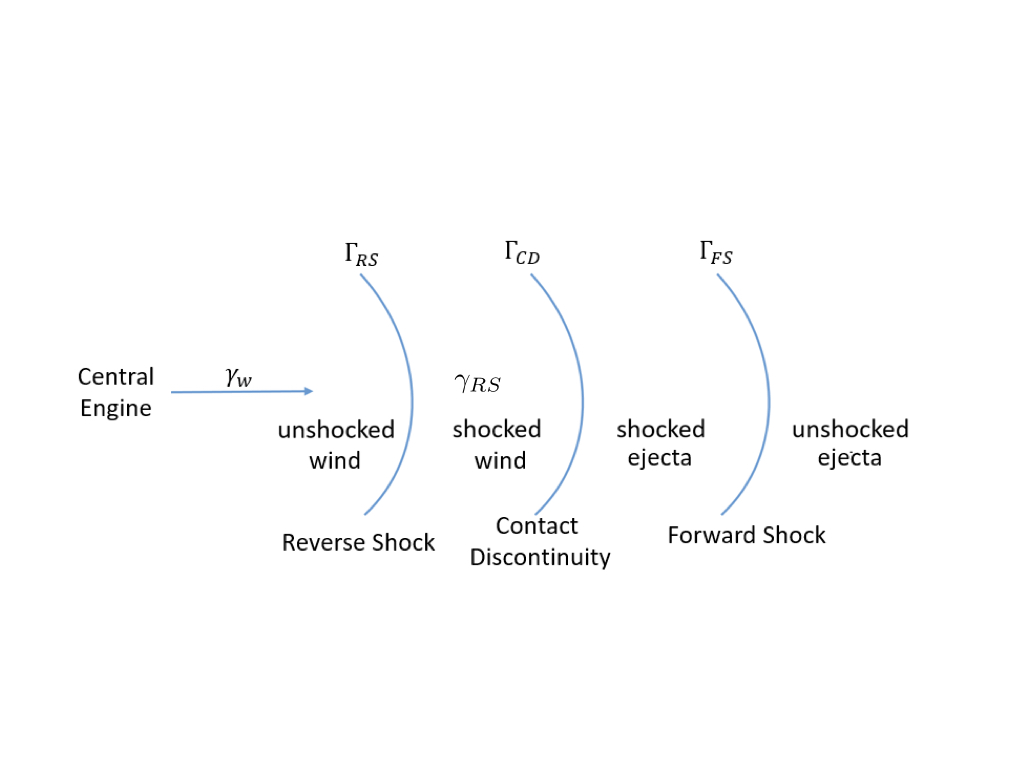
Figure 1: Structure of the wind-ejecta flow. The wind moving with Lorentz factor $\gamma_{w}$ terminates at the reverse shock (RS), which is moving with $\Gamma_{RS}$. The post-RS flow is moving with $\gamma_{RS}\approx\Gamma_{RS}\approx\Gamma_{CD}$ (the Lorentz factor of the contact discontinuity separating wind and ejecta material).

To avoid the mathematical complications, and to demonstrate the essential physical effects most clearly, we assume a simplified dynamics of the second shock, allowing it to propagate with constant velocity. Thus, in the frame of the shock, the magnetic field decreases linearly with time,

$$B^{\prime}=B_{0}^{\prime}\frac{t_{0}^{\prime}}{t^{\prime}}$$ (4)

where time $t_{0}^{\prime}$ and magnetic field is $B_{0}^{\prime}$ are some constants. In the following, we assume that the RS starts to accelerate particles at time $t_{0}^{\prime}$, and we calculate the emission properties of particles injected at the wind termination shock taking into account radiative and adiabatic losses.

2.2 Evolution of the distribution function

As the wind generated by the long-lasting engine starts to interact with the tail part of the flow generated by the initial explosion, the RS forms in the wind, see Fig. 1. Let’s assume that the RS accelerates particles with a power-law distribution,

$$f\left(\gamma^{\prime},t_{i}^{\prime}\right)\propto{\gamma^{\prime}}^{-p}\Theta(\gamma^{\prime}-\gamma_{\text{min}}^{\prime})$$ (5)

where $t_{i}^{\prime}$ is the injection time, $\Theta$ is the step-function, $\gamma$ is the Lorentz factor of the particles, and $\gamma_{\text{min}}^{\prime}$ is the minimum Lorentz factor of the injected particles. $\gamma_{\text{min}}^{\prime}$ can be estimated as (Kennel & Coroniti, 1984b)

$$\gamma_{\text{min}}^{\prime}\sim\gamma_{RS}\sim\gamma_{w}/2\Gamma_{RS}$$ (6)

(We stress that in the pulsar-wind paradigm the minimal Lorentz factor of accelerated particles $\gamma_{\text{min}}^{\prime}$ scales differently from the matter-dominated fireball case.)

The accelerated particles produce synchrotron emission in the ever-decreasing magnetic field, while also experiencing adiabatic losses. Synchrotron losses are given by the standard relations (e.g. Lang, 1999). To take account of adiabatic losses we note that the conservation of the first adiabatic invariant (constant magnetic flux through the cyclotron orbit) gives

$$\partial_{t^{\prime}}\ln\gamma^{\prime}=\frac{1}{2}\partial_{t^{\prime}}\ln B^{\prime}$$ (7)

(thus, we assume that that magnetic field is dominated by the large-scale toroidal field).

Using Eqn. (4) for the evolution of the field, the evolution of a particles’ Lorentz factor follows

$$\frac{{d}\gamma^{\prime}}{{dt^{\prime}}}=-\frac{\tilde{C}_{1}{B_{0}^{\prime}}^{2}{\gamma^{\prime}}^{2}}{{t^{\prime}}^{2}}-\frac{\gamma^{\prime}}{2t^{\prime}}\mbox{}$$

$$\tilde{C}_{1}=\frac{\sigma_{T}{t_{0}^{\prime}}^{2}}{6{\pi m_{e}c}}$$ (8)

where $\sigma_{T}$ is the Thomson cross-section and $t_{0}^{\prime}$ is some reference time.

Solving for the evolution of the particles’ energy in the flow frame,

$$\frac{1}{\gamma^{\prime}}=\frac{2\tilde{C}_{1}{B_{0}^{\prime}}^{2}}{3t^{\prime}}\left(\left(\frac{t^{\prime}}{{t}_{i}^{\prime}}\right)^{3/2}-1\right)+\frac{1}{\gamma_{i}^{\prime}}\sqrt{\frac{t^{\prime}}{t_{i}^{\prime}}},$$ (9)

we can derive the evolution of a distribution function (the Green’s function) (e.g. Kardashev, 1962; Kennel & Coroniti, 1984b)

$$G(\gamma^{\prime},t^{\prime},t_{i}^{\prime})=\left\{\begin{array}[]{cc}{\gamma^{\prime}}^{-p}\left(\frac{t_{i}^{\prime}}{t^{\prime}}\right)^{\frac{p-1}{2}}\left(1-\frac{2}{3}\tilde{C}_{1}{B_{0}^{\prime}}^{2}\gamma_{w}^{\prime}\sqrt{t^{\prime}}\left(\frac{1}{{t_{i}^{\prime}}^{3/2}}-\frac{1}{{t^{\prime}}^{3/2}}\right)\right)^{p-2},&{\gamma_{\text{low}}^{\prime}<\gamma^{\prime}<\gamma_{\text{up}}^{\prime}}\\ 0,&{else}\\ \end{array}\right.\mbox{}$$ (12)

$$\frac{1}{\gamma_{\text{low}}^{\prime}}=\frac{2\tilde{C}_{1}{B_{0}^{\prime}}^{2}}{3t^{\prime}}\left(\left(\frac{t^{\prime}}{t_{i}^{\prime}}\right)^{3/2}-1\right)+\frac{1}{\gamma_{min}^{\prime}}\sqrt{\frac{t^{\prime}}{t_{i}^{\prime}}}\mbox{}$$

$$\frac{1}{\gamma_{\text{up}}^{\prime}}=\frac{2\tilde{C}_{1}{B_{0}^{\prime}}^{2}}{3t^{\prime}}\left(\left(\frac{t^{\prime}}{t_{i}^{\prime}}\right)^{3/2}-1\right)$$ (13)

where $\gamma_{\text{low}}^{\prime}$ is a lower bound of Lorentz factor due to minimum Lorentz factor at injection and $\gamma_{\text{up}}^{\prime}$ is an upper bound of Lorentz factor due to cooling.

Once we know the evolution of the distribution function injected at time $t_{i}^{\prime}$, we can use the Green’s function to derive the total distribution function by integrating over the injection times

$${N}(\gamma^{\prime},t^{\prime})\propto\int_{t_{i}^{\prime}}^{t^{\prime}}\dot{n}(t_{i}^{\prime})G(\gamma^{\prime},t^{\prime},t_{i}^{\prime})dt_{i}^{\prime}$$ (14)

where $\dot{n}(t_{i}^{\prime})$ is the injection rate (assumed to the constant below).

2.3 Observed intensity

The intensity observed at each moment depends on the intrinsic luminosity, the geometry of the flow, relativistic, and time-of-flight effects (e.g. Fenimore et al., 1996; Nakar et al., 2003; Piran, 2004).

The intrinsic emissivity at time $t^{\prime}$ depends on the distribution function $N$ and synchrotron power $P_{\omega}$:

$$L^{\prime}(\omega^{\prime},t^{\prime})=\int\int{N_{A}(\gamma^{\prime},t^{\prime})P_{\omega}(\omega^{\prime})}\,d\gamma^{\prime}dA^{\prime}$$ (15)

where $N_{A}$, the number of particles per unit area, is defined as $N_{A}=N/A=N/(2\pi{r^{\prime}}^{2}(1-\cos\theta_{j}))$, $P(\omega^{\prime})$ is the power per unit frequency emitted by each electron, and $dA^{\prime}$ is the surface differential (unlike Fenimore et al., 1996, we do not have extra $\cos\theta$ in the expression for the area since we use volumetric emissivity, not emissivity from a surface).

We assume that the observer is located on the symmetry axis and that the active part of the RS occupies angle $\theta_{j}$ to the line of sight. The emitted power is then

$$L^{\prime}(\omega^{\prime},t^{\prime})=\int_{0}^{\theta_{j}}\int_{\gamma_{\min}^{\prime}}^{\infty}N_{A}(\gamma^{\prime},t^{\prime})P(\omega^{\prime})d\gamma^{\prime}2\pi{r^{\prime}}^{2}\sin(\theta)d\theta$$ (16)

Figure 2: The illustration of $N_{A}$. We are looking for the number of particles with the angle from $\theta$ to $\theta+\delta\theta$. $N_{A}$ is the number of particles within a unit surface element.

Figure 3: Illustration of the jet opening angle $\theta_{j}$ and calculations of the relation 20. The first light emitted from the central point r=0, which observed at the observed time 0. At the time t, a photon emitted from the location $r=r_{em}$ and angle $\theta$, which observed at $T_{ob}$. The distance between the central point and the observer is assumed to be D. The emission is produced only within the opening angle $\theta_{j}$. $\theta_{i}$ corresponds to an arbitrary place within the opening angle $\theta_{j}$. If the central engine produces an explosion, we would expect the emission from a jet front surface occurs at the same time $t$ in the lab frame. However, in the observed frame, the emission in the jet front surface occurs at a different time (the emission at the emission angle $\theta_{i}$ will occur at $T_{i}$, but the emission at the emission angle $\theta_{j}$ will occur at $T_{j}$). We assume that the observer is looking along the symmetric axis of the jet.

The relation above can be derived from the model shown in Fig. 3. In the lab frame, the first light emitted from the central point and observed at time D/c. At the time t, the ejected particle moves to the location of the radius $r=r_{em}=vt$ and the angle $\theta$. At the same time, a photon is emitted. The time of traveling between the location of the emission and the observer is

$$\Delta t=\frac{\sqrt{\left(D-r_{em}\cos\theta\right)^{2}+\left(r_{em}\sin\theta\right)^{2}}}{c}$$ (17)

The observed time is the difference between the observation of the first light and the light emitted at time t, which can be written as

$$T_{ob}=t+\Delta t-D/c=t+\frac{\sqrt{\left(D-r_{em}\cos\theta\right)^{2}+\left(r_{em}\sin\theta\right)^{2}}}{c}-D/c=t\left(1-\beta\cos\theta\right)$$ (18)

under the assumption of $r_{em}\ll D$.

Photons seen by a distant observer at times $T_{ob}$ are emitted at different radii and angles $\theta$. To take account of the time of flight effects, we note that the distance between the initial explosion point and an emission point $(r^{\prime},\theta)$ is $r^{\prime}=vt^{\prime}=vT_{ob}(1-\beta\cos(\theta))^{-1}\gamma_{RS}^{-1}$, where $T_{ob}$ is the observed time. Supposed that a photon was emitted from the distance $r^{\prime}$ and angle $\theta=0$ at time $t^{\prime}$, and at the same time, the other photon was emitted from the distance $r^{\prime}$ and any arbitrary angle $\theta=\theta_{i}<\theta_{j}$. These two photons will be observed at time $T_{0}$ and $T_{\theta_{i}}$, then the relation between $T_{0}$ and $T_{\theta_{i}}$ is given by:

$$r^{\prime}=vt^{\prime}=\frac{vT_{0}}{(1-\beta)\gamma_{RS}}=\frac{vT_{\theta_{i}}}{(1-\beta\cos(\theta_{i}))\gamma_{RS}}$$ (19)

where, the time $t^{\prime}$ measured in the fluid frame, and the corresponding observe time $T_{ob}$, is a function of $\theta$ and $t^{\prime}$:

$$T_{ob}=t\left(1-\beta\cos\theta\right)=t^{\prime}\left(1-\beta\cos\theta\right)\gamma_{RS}$$ (20)

Taking the derivative of Eqn. (20) we find

$$\sin(\theta)d\theta=-\frac{T_{\text{ob}}}{{t^{\prime}}^{2}\beta\gamma_{RS}}dt^{\prime}\approx-\frac{T_{\text{ob}}}{{t^{\prime}}^{2}\gamma_{RS}}dt^{\prime}$$ (21)

Substitute the relation (21) into (16), the observed luminosity becomes

$$L^{\prime}(T_{ob},\omega^{\prime})\approx\int_{t_{\theta^{\prime}=0}^{\prime}}^{t_{\theta^{\prime}=\theta_{j}}^{\prime}}\int_{\gamma_{\min}^{\prime}}^{\infty}\frac{2\pi c^{2}T_{ob}}{\gamma_{RS}}\times N_{A}(\gamma^{\prime},t^{\prime})P(\omega^{\prime})d\gamma^{\prime}dt^{\prime}$$ (22)

To understand the Eqn. (22), the radiation observed at $T_{ob}$ corresponds to the emission angle from $0$ to $\theta_{j}$, which also corresponds to the emission time $t_{\theta^{\prime}=0}^{\prime}={T_{ob}}/{(1-\beta)\gamma_{RS}}$ to $t_{\theta^{\prime}=\theta_{j}}^{\prime}={T_{ob}}/{(1-\beta\cos\theta_{j})\gamma_{RS}}$. So we need to integrate the emissivity function over the range of the emission angle, or integrate the emissivity function over the range of the emission time from $t_{\theta^{\prime}=0}^{\prime}={T_{ob}}/{(1-\beta)\gamma_{RS}}$ to $t_{\theta^{\prime}=\theta_{j}}^{\prime}={T_{ob}}/{(1-\beta\cos\theta_{j})\gamma_{RS}}$.

Figure 4: The illustration of the model. For the photons observed at $T_{ob}$, they are emitted at different times $t^{\prime}$ in the fluid frame and different angles $\theta$.

Figure 5: The illustration of the model. For the photon observed at $T_{ob}$, they are not emitted from a spherical shell. The distance from the central point (i.e., the time in fluid frame) and the angle respect to the line of sight are related via equation $T_{ob}=t\left(1-\beta\cos\theta\right)=t^{\prime}\left(1-\beta\cos\theta\right)\gamma_{RS}$

Finally, taking into account Doppler effects (Doppler shift $\omega=\delta\omega^{\prime}$ and the intensity boost $I_{\omega}\left(\omega\right)=\delta^{3}I_{\omega^{\prime}}^{\prime}\left(\omega^{\prime}\right)$; where $\delta$ is the Doppler factor $\delta=1/({\gamma_{RS}\left(1-\beta\cos\theta\right)})$), substitute the relation $t^{\prime}={T_{\text{ob}}}/{(1-\beta\cos(\theta))\gamma_{RS}}$ into Eqn.(22) we finally arrive at the equation for the observed spectral luminosity:

$$F_{\omega}=\int_{\frac{T_{\text{ob}}}{(1-\beta\cos(\theta_{j}))\gamma_{RS}}}^{\frac{T_{\text{ob}}}{(1-\beta)\gamma_{RS}}}\int_{\gamma_{\min}^{\prime}}^{\infty}\frac{1}{2\gamma_{RS}}c^{2}D^{-2}T_{\text{ob}}\delta^{3}N_{A}P(\omega/\delta)d\gamma^{\prime}dt^{\prime}$$ (23)

where $D$ is the distance to the GRB.

3 Results

In the following, we apply the general relations derived above to the three specific problem: (i) origin of plateaus in afterglow light curves and (ii) sudden drops in the afterglow light curves §3.1; (iii) afterglow flares, §3.2. For numerical estimates, we assume the redshift $z=1$, the Lorentz factor of the wind $\gamma_{w}=5\times 10^{5}$, the wind luminosity $L_{w}=10^{46}$ erg/s, the initial injection time $t_{0}^{\prime}=10^{5}$s (in jet frame), the power law index of particle distribution $p=2.2$, $\Gamma_{CD}\approx\gamma_{RS}$, and the viewing angle is 0 (observer on the axis) for all calculations.

3.1 Plateaus and sudden intensity drops in afterglow light curves

Particles accelerated at the RS emit in the fast cooling regime. The resulting synchrotron luminosity $L_{s}$ is approximately proportional to the wind luminosity $L_{w}$, as discussed by Lyutikov & Camilo Jaramillo (2017). (For highly magnetized winds with $\sigma\gg 1$ the RS emissivity is only mildly suppressed, by high magnetization, $\propto 1/\sqrt{\sigma}$, due to the fact that higher sigma shocks propagate faster with respect to the wind.) Thus, the constant wind will produce a nearly constant light curve: plateaus are natural consequences in our model in the case of constant long-lasting wind, see Fig. 6. At the early times all light curves show a nearly constant evolution with time, a plateau, with flux $\propto t_{ob}^{-0.1}$. A slight temporal decrease is due to the fact that magnetic field at the RS decreases with time so that particles emit less efficiently. This observed temporal decrease is flatter than what is typically observed, $\propto t_{ob}^{-\alpha_{2}}$ with $\alpha_{2}=0.5-1$ (Nousek et al., 2006). A steeper decrease can be easily accommodated due to the decreasing wind power. This explains the plateaus.

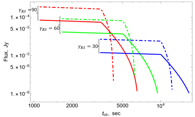
Figure 6: The light curve at 100 KeV for different Lorentz factors of the post-RS flow and different jet angles $1/\gamma_{RS}$ (solid lines) and $1/2\gamma_{RS}$ (dotted-dash lines). Note that for $\theta_{j}<1/\gamma_{RS}$ the drop in intensity is extremely fast.

Next we assume that the central engine suddenly stops operating. This process could be due to the collapse of a neutron star into a black hole or sudden depletion of an accretion disk. At a later time, when the “tail” of the wind reaches the termination shock, acceleration stops. Let the injection terminate at a some time $t_{\text{stop}}^{\prime}$. The distribution function in the shocked part of the wind then become

$${N}(\gamma^{\prime},t^{\prime})\propto\int_{t_{0}^{\prime}}^{\min(t^{\prime},t_{\text{stop}}^{\prime})}G(\gamma^{\prime},t^{\prime},t_{i}^{\prime})dt_{i}^{\prime}$$ (24)

Fig. 7 shows the evolution of the distribution function by assuming the Lorentz factor of RS $\gamma_{RS}=90$, and the injection is stopped at time $t_{\text{stop}}^{\prime}=1.5\times 10^{5}$s (in this case, the $T_{\text{ob,stop}}=833$s in the observer’s frame). The number of high energy particles drops sharply right after the injection is stopped: particles lose their energy via synchrotron radiation and adiabatic expansion in fast cooling regime.

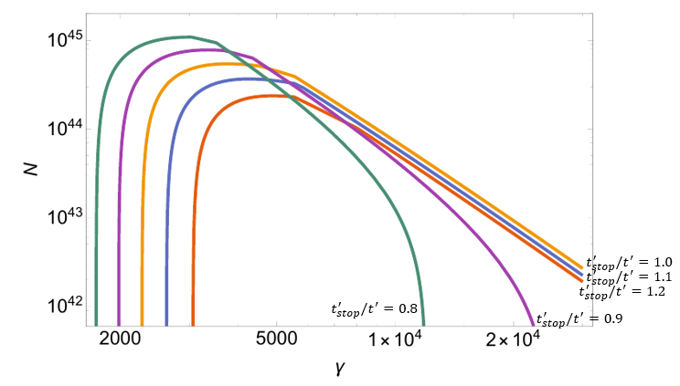
Figure 7: Evolution of the distribution function. Here we take account the effect of radiation loss and adiabatic expansion. In our calculation, the Lorentz factor of RS $\gamma_{RS}=90$, and the injection is stopped at time $t_{\text{stop}}^{\prime}=1.5\times 10^{5}$s, $\gamma_{\min}=\gamma_{w}/\gamma_{RS}=5556$, initial magnetic field $B_{0}=2.1$G. The times are measured in fluid frame at $t_{\text{stop}}^{\prime}/t^{\prime}=1.2,1.1,1.0,0.9,0.8$ from red to green curves.

The resulting light curves are plotted in Fig. 6. We assume post-RS flow $\gamma_{RS}=30,\,60,\,90$ and two jet opening angles of $\sim\gamma_{RS}^{-1}$ and $\sim(1/2)\gamma_{RS}^{-1}$. These particular choices of $\theta_{j}$ are motivated by our expectation that sudden switch-off of the acceleration at the RS will lead to fast decays in the observed flux (in the fast cooling regime).

The injection is stopped at a fixed time in the fluid frame, corresponding to $t_{0}^{\prime}=6\times 10^{5}$s. There is a sudden drop of intensity when the injection is stopped ($T_{\text{ob}}=10000$s for blue curve, $T_{\text{ob}}=5000$s for green curve, and $T_{\text{ob}}=3333$s for red curve). Blue curve has $\gamma_{RS}=30$, $\gamma_{\min}=\gamma_{\text{w}}/\gamma_{RS}=16667$, initial magnetic field $B_{0}$ = 6.4G; green curve has $\gamma_{RS}=60$, $\gamma_{\min}=\gamma_{w}/\gamma_{RS}=8333$, initial magnetic field $B_{0}$=3.2G; red curve has $\gamma_{RS}=90$, $\gamma_{\min}=\gamma_{w}/\gamma_{RS}=5556$, initial magnetic field $B_{0}$ = 2.1G. Here we assume $B_{0}\propto{\gamma_{RS}}^{-1}$ for our calculations. Smaller jet angle produce sharper drop.

In the simplest qualitative explanation, consider a shell of radius $r_{em}$ extending to a finite angle $\theta_{j}$ and producing an instantaneous flash of emission (instantaneous is an approximation to the fast cooling regime). The observed light curve is then Fenimore et al. (1996)

$$\propto\left\{\begin{array}[]{cc}\left(\frac{T_{ob}}{T_{0}}\right)^{-(\alpha+2)},&0<T_{ob}<\frac{r_{em}/c}{2}\theta_{j}^{2}\\ 0&\frac{r_{em}/c}{2}\theta_{j}^{2}<T_{ob}\end{array}\right.$$ (25)

where $T_{0}=\frac{r_{em}/c}{2\gamma_{RS}^{2}}$ and $\alpha$ is the spectral index. Thus, for $\theta_{j}>1/\gamma_{RS}$ the observed duration of a pulse is $\sim T_{0}$, while for $\theta_{j}<1/\gamma_{RS}$ the pulse lasts much shorter, $\sim T_{0}(\theta_{j}\gamma_{RS})^{2}\ll T_{0}$. Thus, in this case a drop in intensity is faster than what would be expected in either faster shocks or shocks producing emission in slowly cooling regime.

3.2 Afterglow flares

Next, we investigate the possibility that afterglow flares are produced due to the variations in wind power. We re-consider the case of $\gamma_{RS}=60$ (the green curve in Fig. 6), but set the ejected power at two, four, and eight times larger than the average power for a short period of time from $2.4\times 10^{5}$s to $2.5\times 10^{5}$s. We consider the two cases: the wide jet angle ($\theta_{j}=1/\gamma_{RS}$) and the narrow jet angle ($\theta_{j}=1/2\gamma_{RS}$). The corresponding light curves are plotted in Fig. 8.

Light curves show a sharp rise around $T_{ob}=2000$ corresponding to the increased ejected power $t=2.4\times 10^{5}$s at emission angle $\theta=0$, followed by a sharp drop around $T_{ob}=4000$s for the case of wide jet and $T_{ob}=2500$s for the case of narrow jet (which corresponds to the ending time of the increased ejected power $t=2.5\times 10^{5}$s at emission angle $\theta=\theta_{j}$). Bright flares are clearly seen. Importantly, the corresponding total injected energy is only $\sim 1\%,\,5\%$ and $10\%$ larger than the averaged value. The magnitude of the rise in flux is less than the magnitude of the rise in ejected power (e.g. the rise in ejected power by a factor eight only gives the rise in flux by a factor two), due to the fact that the emission from the increased ejected power from different angles is spread out in observer time. Thus, variations in the wind power, with minor total energy input, can produce bright afterglow flares.

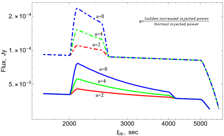
Figure 8: Afterglow flares due to variations in wind luminosity for the case $\gamma_{RS}=60$ (green curve in the Fig. 6). The ejected power is increased by factors $a=2,4,8$ for a short period from $2.4\times 10^{5}$s to $2.5\times 10^{5}$s (in the fluid frame). Solid lines are for $\theta_{j}=\gamma_{RS}$, dashed lines are for $\theta_{j}=1/2\gamma_{RS}$. The relative shift of intensities between the plots for two opening angles is due to our parametrization of the injected power (constant total power).

4 Discussion

In this paper, we calculate emission properties expected from (non-stationary) particle injection at the termination shock of long-lasting GRB engines. We assume a “pulsar paradigm”: the central engine produces ultra-relativistic, highly magnetized wind with particles accelerated at the wind termination shock (Kennel & Coroniti, 1984c). (In contrast, a number of authors, e.g., Rees & Meszaros, 1994, discussed long-lasting engine that produces colliding shells, in analogy with the fireball model for the prompt emission).

The key advantages of the model are high radiation efficiency, and the ability to produce fast temporal variations. We can reproduce

• Afterglow plateaus: in the fast cooling regime the emitted power is comparable to the wind power. Hence, only mild wind luminosity $L_{w}\sim 10^{46}$ erg s^-1 is required

• Sudden drops in afterglow curves: if the central engine stops operating, and if at the corresponding moment the Lorentz factor of the RS is of the order of the jet angle, a sudden drop in intensity will be observed.

• Afterglow flares: if the wind intensity varies, this leads to the sharp variations of afterglow luminosities. Importantly, a total injected energy is small compared to the total energy of the explosion.

Our model may provide explanations to other problems in GRBs’ afterglow. (i) “Naked GRBs problem” (Page et al., 2006; Vetere et al., 2008): if the explosion does not produce a long-lasting wind, then there will be no X-ray afterglow since RS reflects the properties of wind. (ii) “Missing orphan afterglows”: both prompt emission and afterglow emission arise from the engine-powered flow, so they may have similar collimation properties.

Finally, let us comment on another conceptual point: analytical and numerical studies of relativistic double explosions (Lyutikov & Camilo Jaramillo, 2017; Lyutikov, 2017; Barkov & Lyutikov, 2020) assumed that the initial FS has reached a self-similar Blandford & McKee (1976) stage. This is an important (and not fully justified) simplification: in reality one expects that the dynamics of the second set of shocks will be influenced by the density structure of ejecta, resulting in shell-induced variations of the Lorentz factor of the contact discontinuity and of the reverse shock. This will produce additional variations of the RS emissivity.

This research was supported by NASA Swift grant 1619001.

References

- Barkov & Lyutikov (2020) Barkov, M. & Lyutikov, M. 2020, arXiv e-prints, arXiv:2004.13600
- Blandford & McKee (1976) Blandford, R. D. & McKee, C. F. 1976, Physics of Fluids, 19, 1130
- Fenimore et al. (1996) Fenimore, E. E., Madras, C. D., & Nayakshin, S. 1996, ApJ, 473, 998
- Hoshino et al. (1992) Hoshino, M., Arons, J., Gallant, Y. A., & Langdon, A. B. 1992, ApJ, 390, 454
- Johnson & McKee (1971) Johnson, M. H. & McKee, C. F. 1971, Phys. Rev. D, 3, 858
- Kardashev (1962) Kardashev, N. S. 1962, Soviet Ast., 6, 317
- Kennel & Coroniti (1984a) Kennel, C. F. & Coroniti, F. V. 1984a, ApJ, 283, 694
- Kennel & Coroniti (1984b) —. 1984b, ApJ, 283, 710
- Kennel & Coroniti (1984c) —. 1984c, ApJ, 283, 710
- Krimm et al. (2007a) Krimm, H. A., Boyd, P., Mangano, V., Marshall, F., Palmer, D. M., Roming, P. W. A., Sbarufatti, B., Barthelmy, S. D., Burrows, D. N., & Gehrels, N. 2007a, GCN Report, 26
- Krimm et al. (2007b) Krimm, H. A., Boyd, P., Mangano, V., Marshall, F., Sbarufatti, B., & Gehrels, N. 2007b, GRB Coordinates Network, 6014
- Lang (1999) Lang, K. R. 1999, Astrophysical formulae
- Langdon et al. (1988) Langdon, A. B., Arons, J., & Max, C. E. 1988, Physical Review Letters, 61, 779
- Lyutikov (2006) Lyutikov, M. 2006, New Journal of Physics, 8, 119
- Lyutikov (2009) —. 2009, ArXiv e-prints
- Lyutikov (2010) —. 2010, Phys. Rev. E, 82, 056305
- Lyutikov (2017) —. 2017, Physics of Fluids, 29, 047101
- Lyutikov & Camilo Jaramillo (2017) Lyutikov, M. & Camilo Jaramillo, J. 2017, ApJ, 835, 206
- Mészáros (2006) Mészáros, P. 2006, Reports on Progress in Physics, 69, 2259
- Nakar et al. (2003) Nakar, E., Piran, T., & Granot, J. 2003, New. Astr., 8, 495
- Nousek et al. (2006) Nousek, J. A., Kouveliotou, C., Grupe, D., Page, K. L., Granot, J., Ramirez-Ruiz, E., Patel, S. K., Burrows, D. N., Mangano, V., Barthelmy, S., Beardmore, A. P., Campana, S., Capalbi, M., Chincarini, G., Cusumano, G., Falcone, A. D., Gehrels, N., Giommi, P., Goad, M. R., Godet, O., Hurkett, C. P., Kennea, J. A., Moretti, A., O’Brien, P. T., Osborne, J. P., Romano, P., Tagliaferri, G., & Wells, A. A. 2006, ApJ, 642, 389
- Paczynski (1986) Paczynski, B. 1986, ApJ, 308, L43
- Page et al. (2006) Page, K. L., King, A. R., Levan, A. J., O’Brien, P. T., Osborne, J. P., Barthelmy, S. D., Beardmore, A. P., Burrows, D. N., Campana, S., Gehrels, N., Graham, J., Goad, M. R., Godet, O., Kaneko, Y., Kennea, J. A., Markwardt, C. B., Reichart, D. E., Sakamoto, T., & Tanvir, N. R. 2006, ApJ, 637, L13
- Piran (1999) Piran, T. 1999, Phys. Rep., 314, 575
- Piran (2004) —. 2004, Reviews of Modern Physics, 76, 1143
- Rees & Meszaros (1992) Rees, M. J. & Meszaros, P. 1992, MNRAS, 258, 41P
- Rees & Meszaros (1994) —. 1994, ApJ, 430, L93
- Sari & Piran (1995) Sari, R. & Piran, T. 1995, ApJ, 455, L143
- Sbarufatti et al. (2007) Sbarufatti, B., Mangano, V., Mineo, T., Cusumano, G., & Krimm, H. 2007, GRB Coordinates Network, 6008
- Troja et al. (2007) Troja, E., Cusumano, G., O’Brien, P. T., Zhang, B., Sbarufatti, B., Mangano, V., Willingale, R., Chincarini, G., Osborne, J. P., Marshall, F. E., Burrows, D. N., Campana, S., Gehrels, N., Guidorzi, C., Krimm, H. A., La Parola, V., Liang, E. W., Mineo, T., Moretti, A., Page, K. L., Romano, P., Tagliaferri, G., Zhang, B. B., Page, M. J., & Schady, P. 2007, ApJ, 665, 599
- Vetere et al. (2008) Vetere, L., Burrows, D. N., Gehrels, N., Meszaros, P., Morris, D. C., & Racusin, J. L. 2008, in American Institute of Physics Conference Series, Vol. 1000, American Institute of Physics Conference Series, ed. M. Galassi, D. Palmer, & E. Fenimore, 191–195