Fast Adaptation to New Environments via Policy-Dynamics Value Functions

Abstract

Standard RL algorithms assume fixed environment dynamics and require a significant amount of interaction to adapt to new environments. We introduce Policy-Dynamics Value Functions (PD-VF), a novel approach for rapidly adapting to dynamics different from those previously seen in training. PD-VF explicitly estimates the cumulative reward in a space of policies and environments. An ensemble of conventional RL policies is used to gather experience on training environments, from which embeddings of both policies and environments can be learned. Then, a value function conditioned on both embeddings is trained. At test time, a few actions are sufficient to infer the environment embedding, enabling a policy to be selected by maximizing the learned value function (which requires no additional environment interaction). We show that our method can rapidly adapt to new dynamics on a set of MuJoCo domains. Code available at policy-dynamics-value-functions.

1 Introduction

Deep reinforcement learning (RL) has achieved impressive results on a wide range of complex tasks (Mnih et al., 2015; Silver et al., 2016, 2017, 2018; Jaderberg et al., 2019; Berner et al., 2019; Vinyals et al., 2019). However, recent studies have pointed out that RL agents trained and tested on the same environment tend to overfit to that environment’s idiosyncracies and are unable to generalize to even small perturbations (Whiteson et al., 2011; Rajeswaran et al., 2017; Zhang et al., 2018c, a; Henderson et al., 2018; Cobbe et al., 2019; Raileanu & Rocktäschel, 2020; Song et al., 2020). It is often the case that besides the test environments being different from the train environments, they will also have costly interactions, scarce or unavailable feedback, and irreversible consequences. For example, a self-driving car might have to adjust its behavior depending on weather conditions, or a prosthetic control system might have to adapt to a new human. In these cases it is crucial for RL agents to find and execute appropriate policies as quickly as possible.

Our approach is inspired by Sutton et al. (2011) who introduced the notion of general value functions (GVFs), which can be used to gather knowledge about the world in the form of predictions. A GVF estimates the expected return of an arbitrary policy on a certain task (as defined by a reward function, a termination function and a terminal-reward function). Similarly, in this work, we aim to learn a value function conditioned on elements of a space of policies and tasks, but here, a “task” is specified by the transition function of the MDP instead of the reward function.

More specifically, we propose PD-VF, a novel framework for rapid adaptation to new environment dynamics. PD-VF consists of four phases: (i) a reinforcement learning phase in which individual policies are learned for each environment in our training set using standard RL algorithms, (ii) a self-supervised phase in which trajectories generated by these policies are used to learn embeddings for both policies and environments, (iii) a supervised training phase in which a neural network is used to learn the value function of a certain policy acting in some environment. The network takes as inputs the initial state of the environment, as well as the corresponding policy and environment embeddings (as learned in the previous phase) and is trained with supervision of the cumulative reward obtained during an episode, and finally (iv) an evaluation phase in which, given a new environment, its dynamics embedding is inferred using the first few steps of an episode. Then, a policy is selected by finding the policy embedding that maximizes the learned value function. The selected policy is used to act in the environment until the episode ends.

Our framework uses self-supervised interactions with the environment to learn an embedding space of both dynamics and policies. By learning a value function in the policy-dynamics space, PD-VF can discover useful patterns in the complex relation between a family of environment dynamics, various behaviors, and the expected return. The value function is designed to model non-optimal policies along with optimal policies in given environments so that it can understand how changes in dynamics relate to changes in the return of different policies. PD-VF uses the learned space of dynamics to rapidly embed a new environment in that space using only a few interactions. At test time, PD-VF can evaluate or rank policies (from a certain family) on unseen environments without the need of full rollouts (i.e. it does not require full trajectories or rewards to update the policy). We evaluate our method on a set of continuous control tasks (with varying dynamics) in MuJoCo (Todorov et al., 2012). The dynamics of each task instance are determined by physical parameters such as wind direction or limb length and can be sampled from a continuous or discrete distribution. Performance is evaluated on a single episode at test time to emphasize rapid adaptation. We show that PD-VF outperforms other meta-learning and transfer learning approaches on new environments with unseen dynamics.

2 Related Work

Our work draws inspiration from multiple research areas such as transfer learning (Taylor & Stone, 2009; Higgins et al., 2017), skill and task embedding (Devin et al., 2016; Zhang et al., 2018b; Hausman et al., 2018; Petangoda et al., 2019), and general value functions (Precup et al., 2001; Sutton et al., 2011; White et al., 2012).

Multi-Task and Transfer Learning. Taylor & Stone (2009) presents an overview of transfer learning methods in RL. A popular approach for transfer in RL is multi-task learning (Taylor & Stone, 2009; Teh et al., 2017), a paradigm in which an agent is trained on a family of related tasks. By simultaneously learning about different tasks, the agent can exploit their common structure, which can lead to faster learning and better generalization to unseen tasks from the same family (Taylor & Stone, 2009; Lazaric, 2012; Ammar et al., 2012, 2014; Parisotto et al., 2015; Borsa et al., 2016; Gupta et al., 2017; Andreas et al., 2017; Oh et al., 2017; Hessel et al., 2019). A large body of work has been inspired by the Horde architecture (Sutton et al., 2011), which consists of a number of RL agents with different policies and goals. Each agent is tasked with estimating the value function of a particular policy on a given task, thus collectively representing knowledge about the world. Building on these ideas, other methods leverage the shared dynamics of the tasks (Barreto et al., 2017; Zhang et al., 2017; Madjiheurem & Toni, 2019) or the similarity among value functions and the associated optimal policies (Schaul et al., 2015; Borsa et al., 2018; Hansen et al., 2019; Siriwardhana et al., 2019). These approaches assume the same underlying transition function for all tasks. In contrast, we focus on transferring knowledge across tasks with different dynamics.

Meta-Learning and Robust Transfer. A popular approach for fast adaptation to new environments is meta reinforcement learning (meta RL) (Cully et al., 2015; Finn et al., 2017; Wang et al., 2017; Duan et al., 2016; Xu et al., 2018; Houthooft et al., 2018; Sæmundsson et al., 2018; Nagabandi et al., 2018; Humplik et al., 2019; Rakelly et al., 2019). Meta RL methods have been designed to work well with dense reward and recent work has shown that they struggle to learn from a limited number of interactions and optimization steps at test time (Yang et al., 2019). In contrast, our framework is capable of rapid adaptation to new environment dynamics and does not require dense reward or a large number of interactions to find a good policy. Moreover, PD-VF does not update the model parameters at test time, which makes it less computationally expensive than meta RL. Another common approach for transfer across dynamics is model-based RL, which uses Gaussian processes (GPs) or Bayesian neural networks (BNNs) to estimate the transition function (Doshi-Velez & Konidaris, 2013; Killian et al., 2017). However, such methods require fictional rollouts to train a policy from scratch at test time, which makes them computationally expensive and limits their applicability for real-world tasks. Yao et al. (2018) uses a fully-trained BNN to further optimize latent variables during a single test episode, but requires an optimal policy for each training instance, which makes it harder to scale. Robust transfer methods either require a large number of interactions at test time (Rajeswaran et al., 2017) or assume that the distribution over hidden variables is known or controllable (Paul et al., 2018). An alternative approach was proposed by Pinto et al. (2017) who use an adversary to perturb the system, achieving robust transfer across physical parameters such as friction or mass.

Skill and Task Embeddings. A large body of work proposes the use of learned skill and task embeddings for transfer in RL (Da Silva et al., 2012; Sahni et al., 2017; Oh et al., 2017; Gupta et al., 2017; Hausman et al., 2018; He et al., 2018). For example, Hausman et al. (2018) use approximate variational inference to learn a latent space of skills. Similarly, Arnekvist et al. (2018) learn a stochastic embedding of optimal Q-functions for various skills and train a universal policy conditioned on this embedding. In both Hausman et al. (2018) and Arnekvist et al. (2018), adaptation to a new task is done in the latent space with no further updates to the policy network. Co-Reyes et al. (2018) learn a latent space of low-level skills that can be controlled by a higher-level policy, in the context of hierarchical reinforcement learning. This embedding is learned using a variational autoencoder (Kingma & Welling, 2013) to encode state trajectories and decode states and actions. Zintgraf et al. (2018) use a meta-learning approach to learn a deterministic task embedding. Wang et al. (2017) and Duan et al. (2017) learn embeddings of expert demonstrations to aid imitation learning using variational and deterministic methods, respectively. More recently, Perez et al. (2018) learn dynamic models with auxiliary latent variables and use them for model-predictive control. Zhang et al. (2018b) use separate dynamics and reward modules to learn a task embedding. They show that conditioning a policy on this embedding helps transfer to changes in transition or reward function. While the above approaches might learn embeddings of skills or tasks, none of them leverage both the latent space of policies and that of the environments for estimating the expected return and using it to select an effective policy at test time.

More similar to our work is that of Yang et al. (2019), who also focus on fast adaptation to new environment dynamics and evaluate performance on a single episode at test time. Yang et al. (2019) train an inference model and a probe to estimate the underlying latent variables of the dynamics, which are then used as input to a universal control policy. While similar in scope, our approach is significantly different from that of Yang et al. (2019). Importantly, Yang et al. (2019) does not learn a latent space of policies and instead trains a universal policy on all the environments. Learning a value function in a space of policies and dynamics allows the function approximator to capture relations among dynamics, behaviors (both optimal as well as non-optimal), and rewards that a universal policy cannot learn. Moreover, the learned structure can aid transfer to new dynamics.

3 Policy-Dynamics Value Functions

In this work, we aim to design an approach that can quickly find a good policy in an environment with new and unknown dynamics, after being trained on a family of environments with related dynamics. The problem can be formalized as a family of Markov decision processes (MDPs) defined by $(\mathcal{S},\mathcal{A},\mathcal{T},\mathcal{R},\gamma)$, where $(\mathcal{S},\mathcal{A},\mathcal{R},\gamma)$ are the corresponding state space, action space, reward function, and discount factor. Each instance of the family is a stationary MDP with transition function $\mathcal{T}_{d}(s^{\prime}|s,a)\in\mathcal{T}$. Each $\mathcal{T}_{d}$ has a hidden parameter $d$ that is sampled once from a distribution $\mathcal{D}$ and held constant for that instance (i.e. episode). $\mathcal{T}_{d}$ can be continuous or discrete in $d$. By design, the latent variable $d$ that defines the MDP’s dynamics cannot be observed from individual states.

We present Policy-Dynamics Value Functions (PD-VF), a novel framework for rapid adaptation across such MDPs with different dynamics. PD-VF is an extension of a value function that not only conditions on a state, but also on a policy and a transition function.

A conventional value function $V:\mathcal{S}\rightarrow\mathcal{R}$ is defined as the expected future return from state $s$ of policy $\pi$:

$$V(s)=\mathbb{E}\left[G_{t}|S_{t}=s\right]=\mathbb{E}\left[\sum_{k=t+1}^{T}\gamma^{k}r_{k}|S_{t}=s\right].$$

Formally, we define a policy-dynamics value function or PD-VF as a function $W:\mathcal{S}\times\Pi\times\mathcal{T}\rightarrow\mathcal{R}$ with two auxiliary inputs representing the policy $\pi$ and the dynamics $d$:

$$W(s,\pi,d)=\mathbb{E}\left[G_{t}|S_{t}=s,A_{t}\sim\pi,S_{t+1}\sim\mathcal{T}_{d}\right].$$

3.1 Problem setup

The dynamics distribution $\mathcal{D}$ is partitioned into two disjoint sets $\mathcal{D}_{train}$ and $\mathcal{D}_{test}$. These are used to generate a set of training and test environments, each having different transition functions, drawn from their respective distributions.

Our model is learned on the training environments in three stages: (i) a reinforcement learning phase, (ii) a self-supervised phase and (iii) a supervised phase. The resulting PD-VF model is evaluated on test environments, where it only experiences a single episode in each. This evaluation setting probes PD-VF’s ability to very quickly adapt to previously unseen dynamics.

3.2 Reinforcement Learning Phase

The first phase of training uses standard model-free RL algorithms to acquire experience in the training environments. An ensemble of $N$ policies are trained, each with a different random seed on one of the training environments. For each policy, we save a number of checkpoints at different stages throughout training. Then, we collect trajectories using each of these checkpoints in each of our training environments. This results in experience from a diverse set of policies (some good, some bad) across environments with different dynamics. Importantly, this dataset contains the behaviors of policies in environments they haven’t been trained on. In the next section, we describe how the collected trajectories are used to learn policy and dynamics embeddings.

3.3 Self-Supervised Learning Phase

The goal of this phase is to learn an embedding space of the dynamics that captures variations in the transition function, as well as an embedding space of the policies that captures variations in the agent behavior.

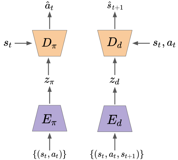
Figure 1: In the self-supervised learning phase, a pair of autoencoders is trained using transitions generated by a diverse set of policies in a set of environments with different dynamics. By exploiting the Markov property of the environment, distinct latent embeddings of the dynamics $z_{d}$ and policy $z_{\pi}$ are produced.

The space of dynamics is learned using an encoder $E_{d}$ parameterised as a Transformer (Vaswani et al., 2017), and a decoder $D_{d}$ parameterised as a feed-forward network. The encoder takes as input a set of transitions $\{(s_{t},a_{t},s_{t+1})\}$ from the first $N_{d}$ steps in each episode and outputs a vector embedding for the dynamics $z_{d}$. The decoder takes as inputs the state $s_{t}$, action $a_{t}$ and dynamics embedding $z_{d}$, and predicts the next state $\hat{s}_{t+1}$. The parameters $\theta_{d}$ and $\phi_{d}$ of the encoder and decoder are trained to minimize the $\ell_{2}$ error of $\hat{s}_{t+1}$ and ${s}_{t+1}$. Formally,

$$z_{d}=E_{d}(\{(s_{t},a_{t},s_{t+1})\};\;\theta_{d})$$

$$\hat{s}_{t+1}=D_{d}(s_{t},a_{t},z_{d};\;\phi_{d}).$$

This arrangement exploits the inductive bias that, conditioned on $d$, the environment is Markovian. By using no positional encoding in the Transformer, the input transitions lack any temporal ordering, thus preserving the Markov property. The decoder receives no historical information (since it is unnecessary in a Markovian setting), so it is forced to embed information about the dynamics into $z_{d}$ to make good predictions. Because the input set contains the actions in each triple, the encoder has no incentive to encode policy information into $z_{d}$. This modeling choice encourages $z_{d}$ to only contain information about the dynamics, rather than the policy used to generate the transitions.

Similarly, the space of policies is learned using an encoder $E_{\pi}$ parameterised as a Transformer and a decoder $D_{\pi}$ parameterised as a feed-forward network. The encoder takes as input a set (again using the Markov property as an inductive bias) of state-action pairs $\{(s_{t},a_{t})\}$ from a full episode and outputs a vector embedding for the policy $z_{d}$. The decoder takes as inputs the state $s_{t}$ and the policy embedding $z_{\pi}$ to predict the action taken by the policy $\hat{a}_{t}$. Since the policy encoder does not have direct access to full environment transitions, $z_{\pi}$ is constrained to capture information about the policy without elements of the dynamics. The parameters $\theta_{\pi}$ and $\phi_{\pi}$ of the encoder and decoder are trained to minimize the $\ell_{2}$ error of $\hat{a}_{t}$ and ${a}_{t}$. Formally,

$$z_{\pi}=E_{\pi}(\{(s_{t},a_{t})\};\;\theta_{\pi})$$

$$\hat{a}_{t}=D_{\pi}(s_{t},z_{\pi};\;\phi_{\pi}).$$

Both the policy and the dynamics embeddings are normalized to have unit $\ell_{2}$-norm.

See Figure 1 for an overview of the self-supervised learning phase.

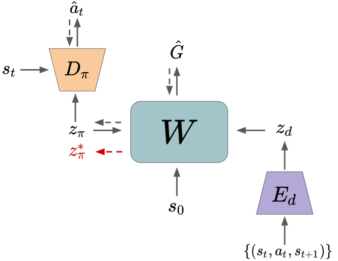
Figure 2: In the supervised learning phase, a parametric value function $W$ is trained to predict the expected return $G$ for an entire space of policies and dynamics. W takes as inputs the initial state $s_{0}$, policy embedding $z_{\pi}$, and dynamics embedding $z_{d}$ (estimated from a small set of transitions). We train $W$ in a supervised fashion, using Monte-Carlo estimates of the expected return $G$ for policy $\pi$ in environment with dynamics $\mathcal{T}_{d}$. At test time, $z_{\pi}$ is optimized to maximize $\hat{G}$ (red dashed arrow), resulting in $z^{*}_{\pi}$ which is then decoded to an actual policy via $D_{\pi}$.

3.4 Supervised Learning Phase

In this phase, the goal is to train an estimator $W$ of the expected return $\hat{G}$ for a space of policies and dynamics. More specifically, $W$ is a function approximator conditioned on the learned policy and dynamics embeddings, $z_{\pi}$ and $z_{d}$.

A central idea of our PD-VF framework is that $W$ provides a scoring function over the policy embedding space. It thus provides a mechanism to allow on-the-fly optimization of $z_{\pi}$ with respect to the estimated return $\hat{G}$, without the need for any environment interaction, given an estimate (or embedding) of the environment’s dynamics. This is key to PD-VF’s ability to rapidly find an effective policy in a new environment, only requiring enough environment interaction to give a reliable estimate of the dynamics embedding $z_{d}$ (just a few steps in practice). We choose $W$ to have a quadratic form to permit easy optimization with respect to $z_{\pi}$:

$$\hat{G}=W(s_{0},z_{\pi},z_{d})=z_{\pi}^{T}\,A(s_{0},z_{d};\psi)\,z_{\pi}.$$

The matrix $A(s_{0},z_{d};\psi)$ is a function of the initial environment state $s_{0}$ as well as the dynamics embedding $z_{d}$. Note that $A$ only needs to model the initial state $s_{0}$ rather than an arbitrary state $s$ since the optimization w.r.t $z_{\pi}$ occurs only once, at the start of an episode. Since $A$ must be Hermitian positive-definite, a feed-forward network with parameters $\psi$ is first used to obtain a lower triangular matrix $L(s_{0},z_{d};\psi)$. Then $A$ is constructed from $LL^{T}$.

Optimizing the policy embedding $z_{\pi}$: The optimization of the policy embedding $z_{\pi}$ has a closed-form solution which is achieved by performing a singular value decomposition, $A=USV^{T}$, and taking the top singular vector of this decomposition $z_{\pi}^{*}$. Unit $\ell_{2}$ normalization is then applied to $z_{\pi}^{*}$. We refer to this vector $z_{\pi}^{*}$ as the optimal policy embedding (OPE) of the PD-VF.

Learning $\psi$ – Initial stage: We collect training data for the PD-VF in the following manner. First, we randomly select a policy and an environment from our training set (described in Section 3.2). Second, we generate full trajectories of that policy in the selected environment and cache the average return obtained across all episodes. This gives us a Monte-Carlo estimate for the expected return of the corresponding policy in that particular environment. Then, we use the first $N_{d}$ steps of that trajectory to infer the dynamics embedding. Similarly, we use the full trajectory to infer the policy embedding (via $E_{\pi}$, not the above optimization procedure). After collecting this data into a buffer, we train the estimator $W$ in a supervised fashion by predicting the expected return $G$ given an initial state $s_{0}$, a policy embedding $z_{\pi}$ and a dynamics embedding $z_{d}$.

Learning $\psi$ – Data Aggregation for the Value Function: For the method to work well, it is important that the learned value function $W$ makes accurate predictions for the entire policy space, and especially for the OPE $z_{\pi}^{*}$ (which correspond to the policies selected to act in the environment). One way to ensure that these estimates are accurate is by adding the OPEs to the training data. After initial training of the PD-VF on the original dataset of policy and dynamics embeddings, we use an iterative algorithm that alternates between collecting a new dataset of OPEs and training the PD-VF on the aggregated data (including the original data as well as data added from all previous iterations). We use early stopping to select the best value function (i.e. the one with the lowest loss) to be used at test time.

Learning $\psi$ – Data Aggregation for the Policy Decoder: Similarly, the policy decoder may poorly estimate an agent’s actions in states not seen during training. Thus, we iteratively train the policy decoder using a combination of the original set of states as well as new states generated by the policy embeddings that maximize the current value function. More specifically, we use the current OPEs (corresponding to the policies that PD-VF thinks are best) as inputs to the policy decoder to generate actions and interact with the environment. Then, we add the states visited by this policy to the data. The policy decoder is trained using the aggregated collection of states which includes both the states visited by the original collection of policies as well as the states visited by the current OPEs selected by the PD-VF.

See Figure 2 for an overview of the supervised learning phase.

3.5 Evaluation Phase

At test time, we want to find a policy that performs well on a single episode of an environment with unseen dynamics. This proceeds as follows: (i) the agent uses one of the pretrained RL policies to act for $N_{d}$ steps; (ii) the generated transitions are then used to infer the dynamics embedding $z_{d}$; (iii) once an estimate of the dynamics is obtained, the matrix $A(s_{0},z_{d};\;\psi)$ can be computed; (iv) we employ the closed-form optimization described above to compute the optimal policy embedding $z_{\pi}^{*}$; (v) the policy decoder, conditioned on the $z_{\pi}^{*}$ embedding, is then used to take actions in the environment until the end of the episode. Note that only a small number of interactions with a new environment is needed in order to adapt, the policy selection being performed internally within the PD-VF model. Performance is evaluated on a single trajectory of each environment instance.

4 Experiments

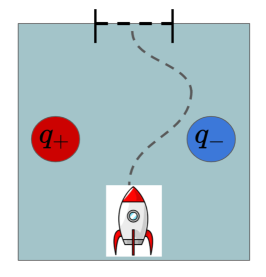
(a) Spaceship

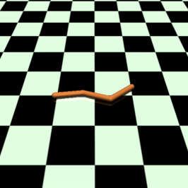
(b) Swimmer

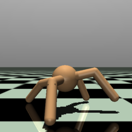
(c) Ant-wind

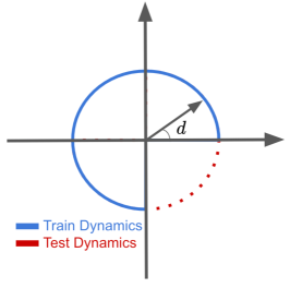
(d) Dynamics

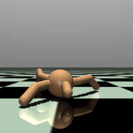
(e) Ant-legs-v1

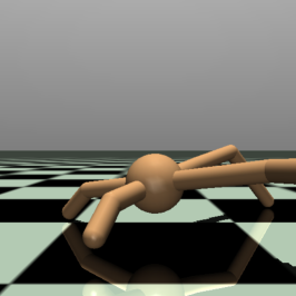
(f) Ant-legs-v2

Figure 3: (a) - (c) illustrate the continuous control domains used for testing adaptation to unseen environment dynamics. In Spaceship, Swimmer, and Ant-wind, the train and test distribution of the dynamics is continuous as illustrated in (d). (e) and (f) show two instances of the Ant-legs task in which limb lengths sampled from a discrete distribution determine the dynamics.

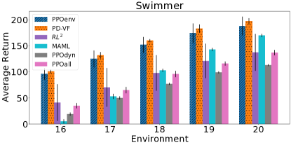
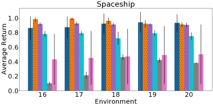
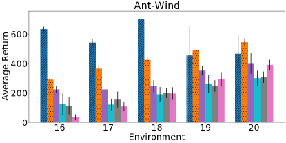
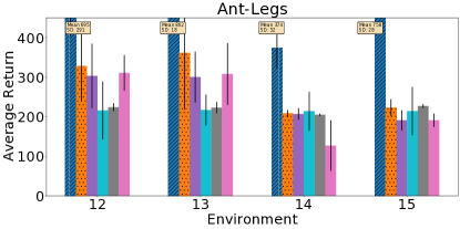
Figure 4: Test Performance. Average return on test environments with unseen dynamics in Swimmer (top-left), Spaceship (top-right), Ant-wind (bottom-left), and Ant-legs (bottom-right) obtained by PD-VF, the upper bound PPOenv, and baselines $RL^{2}$, MAML, PPOdyn, and PPOall. PD-VF outperforms these baselines on most test environments and, in some cases, it is comparable with PPOenv (which was trained directly on the test environments).

4.1 Experimental Setup

We evaluate PD-VF on four continuous control domains, and compare it with an upper bound, four baselines, and four ablations. For each domain, we create a number of environments with different dynamics. Then, we split the set of environments into training and test subsets, so that at test time, the agent has to find a policy that behaves well on unseen dynamics. For all our experiments, we show the mean and standard deviation of the average return (over 100 episodes) across 5 different seeds of each model. The dynamics embeddings are inferred using at most $N_{d}=4$ interactions with the environment.

4.2 Environments

Spaceship is a new continuous control domain designed by us. The task consists of moving a spaceship with a unit point charge from one end of a 2D room through a door at the other end. The action space consists of a fixed-magnitude force vector that is applied at each timestep. The room contains two fixed electric charges that deflect / attract the ship as it moves through the environment (see Figure 3(a)). The polarity and magnitude of these charges are parameterised by $d$ and determine the environment dynamics. The distribution of dynamics $\mathcal{D}$ is chosen to be circular and centered (see Figure 3(d)). Samples $d$ are drawn at intervals of $\pi/10$, each forming a different environment instance with charge configuration $(\cos(d),\sin(d))$. The 5 samples in the range $[\frac{3}{4}2\pi,\ldots,2\pi]$ are held out as evaluation environments, the rest being used for training.

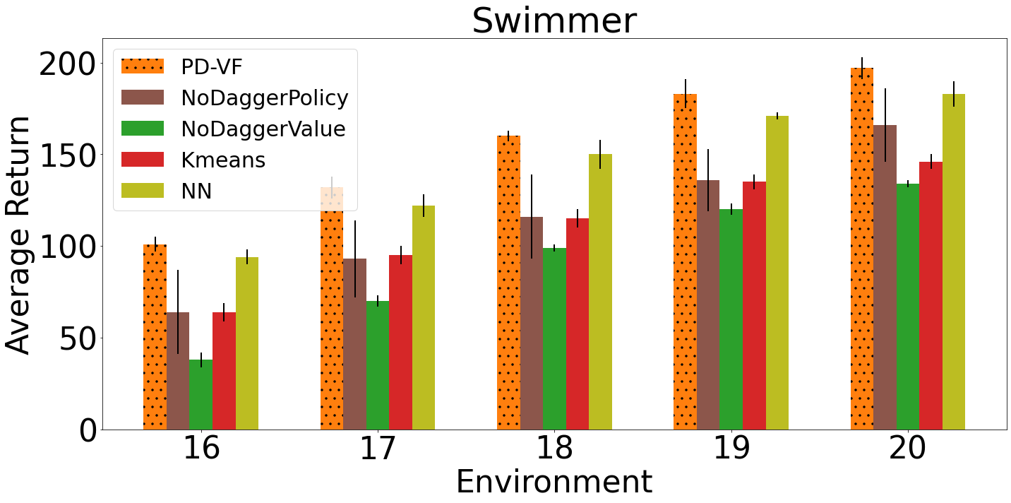
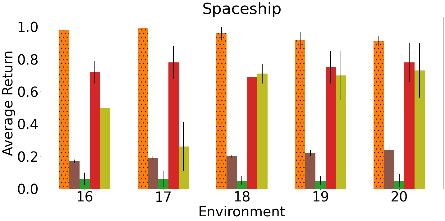
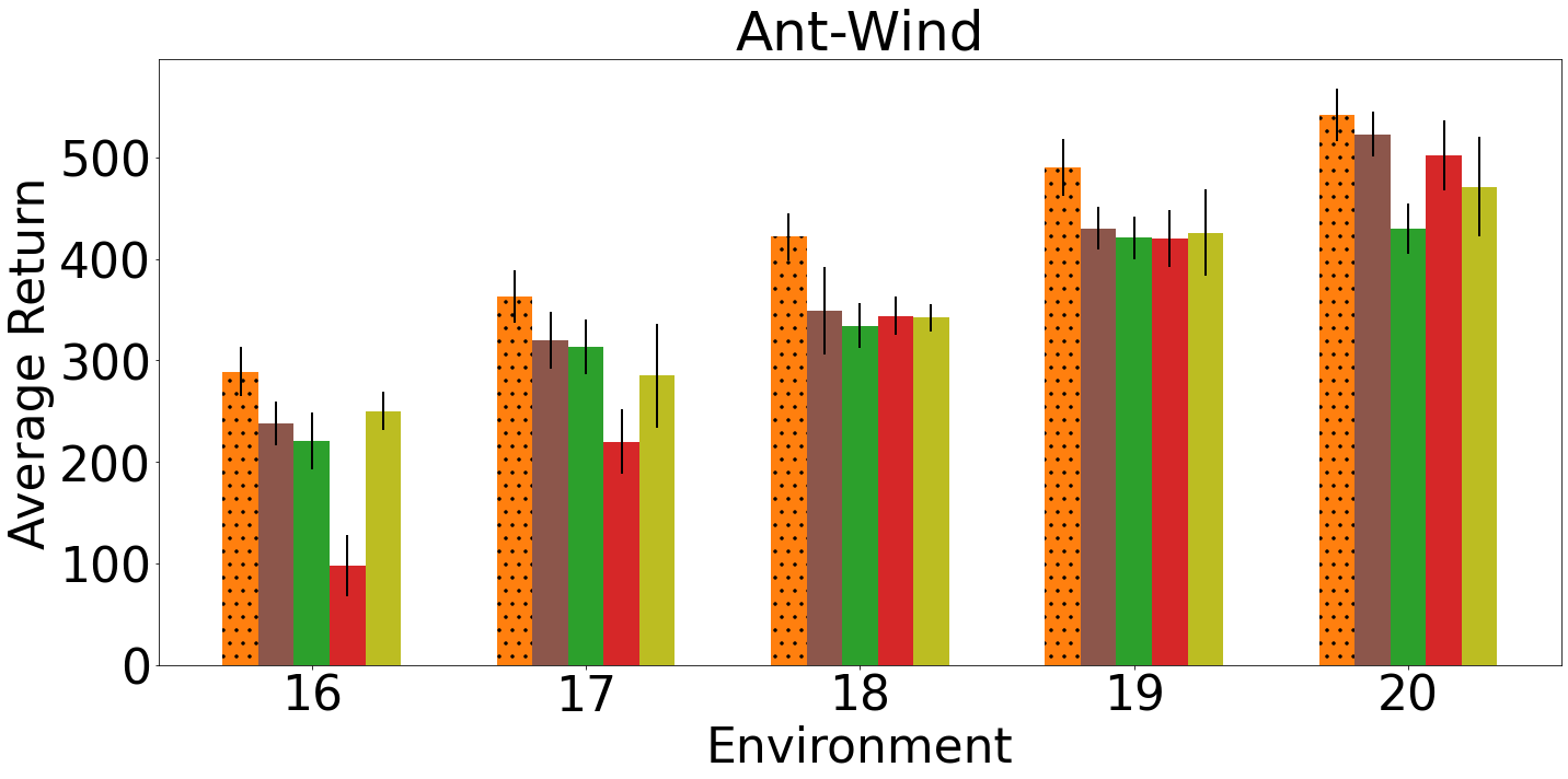
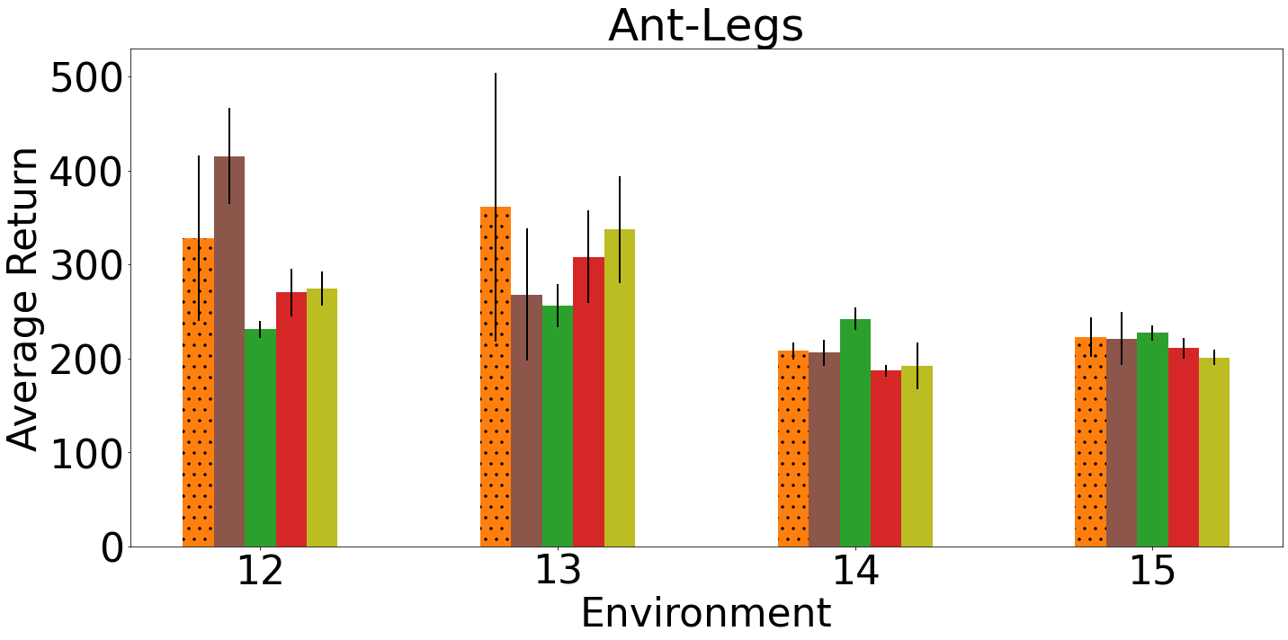
Figure 5: Test Performance. Average return in Swimmer (top-left), Spaceship (top-right), Ant-wind (bottom-left), and Ant-legs (bottom-right) obtained by PD-VF, NoDaggerPolicy, NoDaggerValue, Kmeans, and NN. PD-VF is better than these ablations overall.

Swimmer is a family of environments with varying dynamics based on MuJoCo’s Swimmer-v3 domain (Todorov et al., 2012). The goal is to control a three-link robot in a viscuous fluid to swim forward as fast as possible (Figure 3(b)). The dynamics are determined by a 2D current within the fluid, whose direction changes between environments (but has fixed magnitude). The current direction is determined by an angle $d$, which is sampled in the same manner as for Spaceship above, i.e. train on $3/4$ of all possible directions and hold out the other $1/4$ for evaluation.

Ant-wind is a family of environments based on MuJoCo’s Ant-v3 domain in which the goal is to make a four-legged creature walk forward as fast as possible (Figure 3(c)). The environment dynamics are determined by the direction of a wind $d$, which is sampled from a continuous distribution in the same way as for Swimmer.

Ant-legs is a second task based on MuJoCo’s Ant-v3 domain, in which the dynamics are sampled from a discrete distribution. The training environments are generated by fixing three ankle lengths (short, medium, and long) and generating all possible permutations for the four legs. The length of the ant leg is fixed to medium across all training environments. Symmetries in the training environments are removed by considering ants with the same number of short, medium, or long legs to be the same and choosing one ant from each equivalency class. There are four test environments with both the leg and ankle lengths being either short or long. Note that the test environments are significantly different from all the training ones, thus making Ant-legs a challenging setting for our method. Figures 3(e) and 3(f) show two instances of this environment.

4.3 Baselines

We use PPO (Schulman et al., 2017) as the base RL algorithm for all the baselines and for the reinforcement learning phase of training the PD-VF (Sec. 3.2). We use Adam (Kingma & Ba, 2014) for optimization. All models use the same network architecture for the policy and value functions. For a given environment, all methods use the same number of steps $N_{d}$ (at the beginning of each episode) to infer the embedding of the environment dynamics. Then, they each use a single policy network to act in the environment until the end of the episode. We report the cumulative reward obtained by each method throughout an episodes (in which they first infer the environment dynamics which determines the policy used for acting until the end of the episode). We compare with the following baselines:

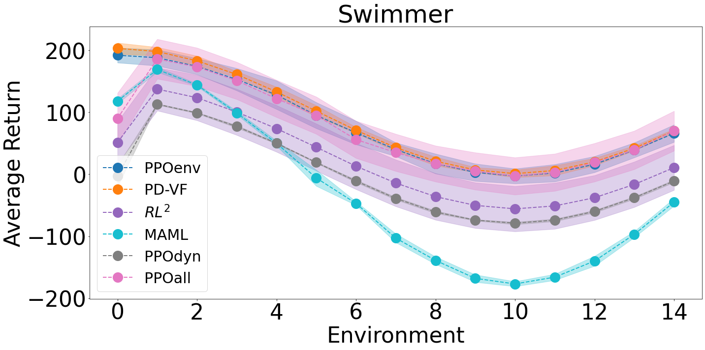
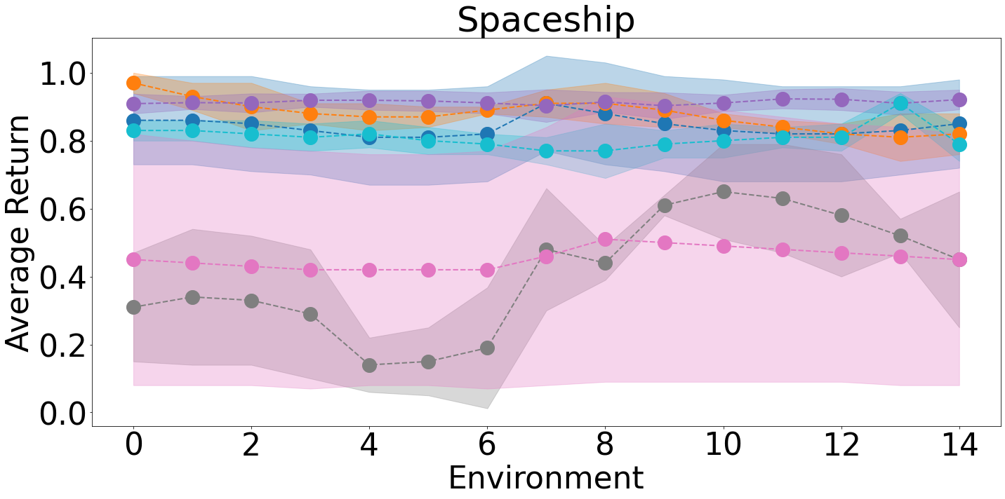
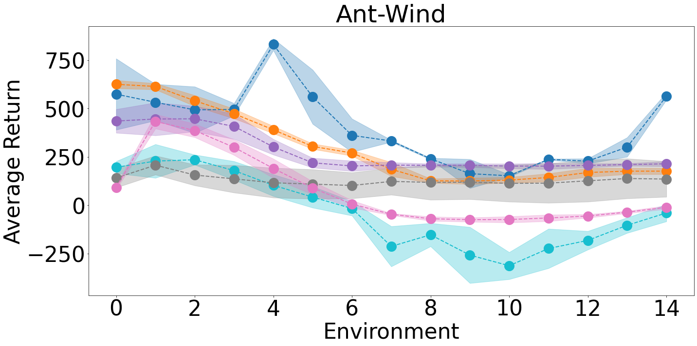
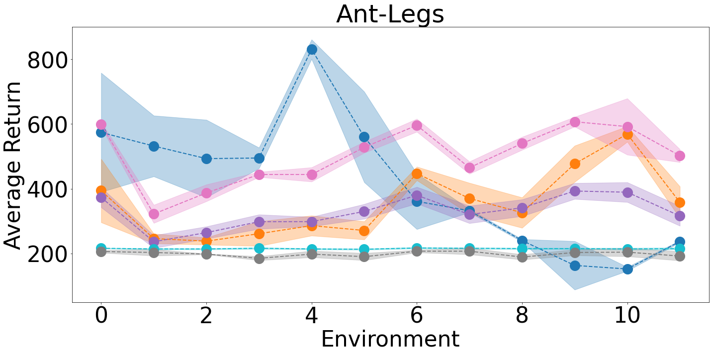
Figure 6: Train Performance. Average return on train environments in Swimmer (top-left), Spaceship (top-right), Ant-wind (bottom-left), and Ant-legs (bottom-right) obtained by PD-VF, the upper bound PPOenv, and baselines $RL^{2}$, MAML, PPOdyn, and PPOall. PD-VF outperforms the baselines and ablations on most test environments and, in some cases, it is comparable with PPOenv (which was trained directly on the test environments). While other methods also perform reasonably well on the training environments, they generalize poorly to new environments with unseen dynamics.

PPOenv trains a PPO policy for each environment in our set. This is used as an upper bound for the other models.

MAML is the meta-learning algorithm from Finn et al. (2017). MAML generally requires some amount of training on the test environments, so to make it more comparable to our method and the other baselines, we allow one gradient step using a trajectory of length $N_{d}$ (i.e. the same length as the one used by PD-VF to infer the embedding of the environment dynamics). Thus, MAML has an advantage over PD-VF which does not make any parameter updates at test time.

$\textbf{RL}^{2}$ is the meta-learning algorithm from Wang et al. (2016) and Duan et al. (2016), which uses a recurrent policy that takes as input the previous action and reward.

PPOdyn trains (using PPO) a single policy network conditioned on the dynamics embedding. At test time, it first infers the dynamics embedding and then conditions the pretrained policy network on that vector. This is a close implementation of the approach in Yang et al. (2019).

PPOall trains a single PPO policy on all the training environments and uses it on the test environments without any additional fine-tuning.

We also compare PD-VF with four ablations:

NN finds the environment that is closest (in Euclidean metric) to the test environment’s embedding and uses the PPOenv policy trained on that environment to act. This ablation aims to tease out the effect of using both the learned space of policies and that of dynamics to adapt to new environments, from that of only using the learned dynamics space.

Kmeans clusters the environment embeddings (using trajectories collected in Section 3.2) into $K$ clusters. Then, for each cluster, we train a new PPO policy on all the environments assigned to that cluster. At test time, we find the closest cluster for the given environment embedding and use the policy corresponding to that cluster to act in the environment.

NoAggValue trains a PD-VF without using dataset aggregation for the value function (see Section 3.4).

NoAggPolicy uses PD-VF without using dataset aggregation for the policy decoder (see Section 3.4).

5 Results

5.1 Adaptation to New Environment Dynamics

As seen in Figures 4 and 5, PD-VF outperforms all other methods on test environments with new dynamics. In some cases (particularly on Spaceship and Swimmer), our approach is comparable to the PPOenv upper bound which was directly trained on the respective test environment (in contrast, PD-VF has never interacted with that environment before). While the strength of PD-VF lies in quickly adapting to new dynamics, its performance on training environments is still comparable to that of the other baselines, as shown in Figure 6. This result is not surprising since current state-of-the-art RL algorithms such as PPO can generally learn good policies for the environments they are trained on, given enough interactions, updates, and the right hyperparamters. However, as predicted, standard model-free RL methods such as the baseline PPOall do not generalize well to environments with dynamics different from the ones experiences during training. Even meta-learning approaches like MAML or $RL^{2}$ struggle to adapt when they are allowed to use only a short trajectory for updating the policy at test time, as is the case here.

But most importantly, PD-VF also outperforms the approaches that use the dynamics embedding such as NN, Kmeans, and PPOdyn. This supports our claim that learning a value function for an entire space of policies (rather than for a single optimal policy as standard RL methods do) can be beneficial for adapting to unseen dynamics. By simultaneously estimating the return of a collection of policies in a family of environments with different but related dynamics, PD-VF can learn how variations in dynamics relate to differences in the performance of various policies. This allows the model to rank different policies and understand that sub-optimal behaviors in certain environments might be optimal in others. Thus, at least in theory, PD-VF has the ability to find policies that are better than the ones seen during training. Our empirical results indicate that this might also hold true in practice. Overall, PD-VF proves to be more robust to changes in dynamics relative to the other methods, especially in completely new environments.

5.2 Analysis of Learned Embeddings

The performance of PD-VF relies on learning useful policy and dynamics embeddings that capture variations in agent behaviors and transition functions, respectively. In this section, we analyze the learned embeddings.

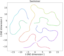
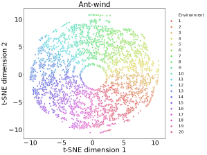
Figure 7: t-SNE plots of the learned environment embeddings $z_{d}$ for Spaceship (a), Swimmer (b), and Ant-wind (c). The color corresponds to the environment that generated the transitions used to encode the corresponding dynamics embeddings. The plot contains embeddings of both train and test environments.

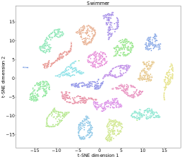
Figure 8: t-SNE plots of the learned policy embeddings $z_{\pi}$ for Spaceship (a), Swimmer (b), and Ant-wind (c). The color corresponds to the policy that generated the transitions used to encode the corresponding policy embeddings. The plot contains embeddings of policies trained on both train and test environments.

Figure 7 shows a t-SNE plot (van der Maaten & Hinton, 2008) of the learned dynamics embeddings on the three continuous control domains used for evaluating our method. Environment $i$ corresponds to dynamics defined by $d=i\times\pi/10$ (i.e. the direction of the wind in Swimmer’s environment 1 is at $\pi/10$ degrees). Environments 1 - 15 are used for training, while 16 - 20 are used for evaluation. The latent space captures the continuous nature of the distribution used to generate the environment dynamics. For example, in Figure 7, one can see the wind direction corresponding to a particular environment, indicating that the learned embedding space uncovers the manifold structure of the true dynamics distribution. Even if, during training, the dynamics model never sees trajectories through the test environments, it is still able to embed them within the 1D manifold, thus preserving smoothness in the latent space.

Similarly, Figure 8 shows the corresponding t-SNE (van der Maaten & Hinton, 2008) of the learned policy embeddings for Spaceship, Swimmer, and Ant. The embeddings are clustered according to the policy that generated them.

6 Discussion and Future Work

In this work, we propose policy-dynamics value functions (PD-VF), a novel framework for fast adaptation to new environment dynamics. The key idea is to learn a value function conditioned on both a policy and a dynamics embedding which are learned in a self-supervised way. At test time, the environment embedding can be inferred from only a few interactions, which allows the selection of a policy that maximizes the learned value function. PD-VF has a number of desirable properties: it leverages the structure in both the policy and the dynamics space to estimate the expected return, it only needs a small number of steps to adapt to unseen dynamics, it does not update any parameters at test time, and it does not require dense reward or long rollouts to find an effective policy in a new environment. Empirical results on a set of continuous control domains show that PD-VF outperforms other methods on unseen dynamics, while being competitive on training environments.

PD-VF opens up many promising directions for future research. First of all, the formulation can be extended to estimate the value function not only for a family of policies and environment dynamics, but also for a family of reward functions. Another avenue for future research is to use a more general class of function approximators (such as neural networks) to parameterise the value estimator instead of a quadratic form. The PD-VF framework can, in principle, also be used to evaluate a family of policies and environments on other metrics of interest besides the expected return, such as, for example, reward variance, agent prosociality, deviation from expert behavior, and so on. Another interesting direction is to integrate additional constraints (or prior knowledge) to the optimization problem (e.g. maximize expected return while only using policies in a certain region of the policy space). As noted by Precup et al. (2001), Sutton et al. (2011), and White et al. (2012), learning about multiple policies in parallel via general value functions can be useful for lifelong learning. Similarly, PD-VF can be a useful tool for an agent to continually gather knowledge about various policies and dynamics in the world. Finally, PD-VF can also be applied to multi-agent settings for adapting to different opponents or teammates whose behaviors determine the environment dynamics.

Appendix A Network Architectures

A.1 Autoencoders

The policy and dynamics autoencoders are parameterised by Transformers using stacked self-attention and point-wise, fully connected layers for the encoder, and a fully connected feed-forward network for the decoder.

Encoders: The encoders consist of one layer composed of two sublayers, followed by another fully connected layer. The first sublayer, is a single-head self-attention mechanism, and the second is a simple fully connected feed-forward network. We employ a residual connection around each of the two sub-layers, followed by layer normalization and dropout. We use a dropout of 0.1 for all experiments. To facilitate these residual connections, all sublayers in the model, as well as the embedding layers, produce outputs of dimension $d_{model}=64$. The second layer of the encoder projects the output of the first layer into the embedding space (from $d_{model}$ to $d_{emb}$).

The policy encoder takes as input a set of state-action pairs $(s_{t},a_{t})$ from an full trajectory and outputs an embedding for the policy.

The dynamics encoder takes as input a set of state-action-next-state tuples $(s_{t},a_{t},s_{t+1})$ from a full trajectory and outputs an embedding for the dynamics.

The dimension of both the policy and dynamics embedding is $d_{emb}=8$ for all environments, with the exception of swimmer which uses a dynamics embedding of dimension 2.

Decoders: The decoder is a simple fully connected feed-forward network with three layers and ReLU activations after the first two layers.

The policy decoder takes as input the state of the environment and the policy embedding (outputted by the policy encoder) and outputs an action (i.e. the predicted action taken by the agent).

The environment decoder takes as input the state of the environment, an action, the dynamics embedding (outputted by the dynamics encoder) and outputs a state (i.e. the predicted next state in the environment).

The dimensions of the states and actions depend on the given environment.

A.2 The Policy-Dynamics Value Function

The Policy-Dynamics Value Function (PD-VF) takes as inputs the initial state of the environment, as well as a policy embedding and a dynamics embedding, and outputs a scalar representing the predicted expected return.

PD-VF is parameterised by a fully connected feed-forward network. First, the environment state and dynamics embedding are concatanated and passed through a linear layer with output dimension 64 followed by a ReLU nonlinearity. The second layer also has output dimension 64 but is followed by a hyperbolic tangent nonlinearity. The output of the second layer is then passed through another linear layer with output dimension equal to the square of the policy embedding dimension which is 64 in this case. Then, the output of this is rearranged in the form of a lower triangular matrix $L$. This matrix is used to construct a Hermitian positive-definite matrix A using the Cholesky decomposition, $A=LL^{T}$. Finally, the value outputted by the network is obtained by computing $z_{\pi}^{T}Az_{\pi}$, where $z_{pi}$ is the policy embedding.

A.3 Baselines

All the pretrained PPO policies as well as all the baselines (except for CondPolicy as explained below) and the ablations use the same actor-critic network architecture. Both the actor and the critic are parameterised two-layer fully connected networks with hidden size 64 and hyperbolic tangent nonlinearities after each layer. Note that the weights are not shared by the two networks. The critic layer has another linear layer on top that outputs the estimated value. The actor network also has a linear layer on top that outputs a vector with the same number of dimensions as the action space. The actions are sampled from a Gaussian distribution with diagonal covariance matrix and means defined by the vector outputted by the actor network. The CondPolicy baseline has a similar architecture. The only difference is the first layer of both the actor and the critic, which has a larger input dimension due to the fact that these networks also take as input the policy embedding (along with the environment state).

Appendix B Training Details

For experiments on Spaceship and Swimmer, we use only $N_{d}=1$ steps to infer the dynamics embedding, while for Ant-wind we use $N_{d}=2$ and for Ant-legs we use $N_{d}=4$. Note that in all four domains, we only need a few steps to infer the environment dynamics, which allows us to quickly find a good policy for acting during the rest of the episode. Consequently, this results in good performance when evaluated on a single episode.

First, we have the reinforcement learning phase, in which we pretrain 5 different initializations of PPO policies in each of the 20 environments in our distribution (both those used for training and those used for evaluation). We train all policies for $3e6$ environment interactions, which we have found to be enough for all of them to converge to a stable expected return.

Then, in the self-supervised learning phase, we use the policies pretrained on the training environments (75 policies for each domain) to generate trajectories through the training environments. For each policy-environment pair, we generate 200 trajectories, half of which are used for training the policy and dynamics autoencodesr and the rest are used for evaluation. We train the autoencoders on this data for a maximum of 200 epochs and we save the models with the lowest evaluation loss. Note that the autoencoders are never trained on trajectories generated in the evaluation environments or by policies pretrained on those environments, but only on data produced by interactions with the training environments.

Once we have the pretrained policy and dynamics autoencoders, we use them for learning the policy-dynamics value function in the supervised training phase. To do this, we again generate 40 trajectories in the training environments (using only the policies pretrained on those environments). Half of these trajectories are used for training the PD-VF, while the rest are used for evaluation. In our experiments, we have found 20 trajectories from each policy-environment pair to be enough for training the model. For each trajectory, a policy embedding is obtained by passing the full trajectory through the policy encoder. Similarly, a corresponding dynamics embedding is obtained for each trajectory by passing the first few $N_{d}$ transitions of that trajectory through the dynamics encoder. The initial state and the return of that trajectory are also recorded. Now we have all the data needed for training the PD-VF with supervision. The PD-VF takes as inputs the initial state, the policy and dynamics embeddings and outputs a prediction for the expected return (corresponding to acting with that policy in the given environment). It is trained with $\ell_{2}$ loss using the observed return. For the initial training stage of the PD-VF, we use 200 epochs, while for the second stage that include data aggregation for the value function and policy decoder, we use 100 epochs. The second stage is repeated a maximum of 20 times (each training for 100 epochs). We select the model that obtains the lowest loss on the evaluation data (out of all the models after each stage). We use this model for probing performace on the evaluation environments.

Appendix C Hyperparameters

For training the PPO policies, as well as the baselines and ablations, we searched for the learning rate in [0.0001, 0.0003, 0.0005, 0.001] and found 0.0003 to work best across the boad. The entropy coefficient was set to 0.0, value loss coefficient 0.5, number of PPO epochs 10, number of PPO steps 2048, number of mini batches 32, gamma 0.99, and generealized advantage estimator coefficient 0.95. We also linearly decay the learning rate. These values were not searched over since they have been previously optimized for MuJoCo domains and have been shown to be robust across these environments.

For MAML, we used the best hyperparameters found in the original paper for MuJoCo, so meta batch size of 20, 10 batches, and 8 workers.

For the dynamics autoencoder, we did a grid search over the learning rate in [0.0001, 0.001, 0.01] and found 0.001 to be best for the dynamics and 0.01 to be best for the policy. We also searched for the right batch size in [8, 32, 256, 2048] and found 8 to work best for the dynamics and 2048 for the policy. We also did grid searches over $d_{emb}\in[2,8,32]$ and found $d_{emb}=8$ for the policy autoencoders and $d_{emb}=2$ for the dynamics autoencoders (except for Ant, in which we use $d_{emb}=8$. We also searched for the hidden dimension of the transformers $d_{model}\in[32,64,128]$ and found $d_{model}=64$ to work best for both the policy and the dynamics embeddings.

For the value function, we tried different values for the number of epochs for the initial training phase $N_{ep,1}\in$ [1000, 500, 200, 100] and for the second training phase $N_{ep,2}\in$ [500, 200, 100] and we found 200 and 100 (i.e. each of the 20 data aggregation stages has 100 epochs) to work best, respectively. We also tried different learning rates from [0.0005, 0.001, 0.005, 0.01] and found 0.005 to be the best. Similarly, we tried batch sizes in [64, 128, 256] and found 128 to be the best.

All the results shown in this paper are obtained using the best hyperparameters found in our grid searches.

Appendix D Environments

D.1 Spaceship Environment

The source code contains the Spaceship domain that we designed, which is wrapped in a gym environment, so it can be easily integrated with any RL algorithm and used to evaluate agents.

The task consists of moving a spaceship with a unit point charge from one end of a 2D room through a door at the other end. The action space consists of a fixed-magnitude force vector that is applied at each timestep. The room contains two fixed electric charges that deflect/attract the ship as it moves through the environment.

At the beginning of each episode, the agentś location is initialized at the center-bottom of the room with coordinates (2.5, 0.2). The target door is always located at the center-top of the room with coordinates (2.5, 5.0). The size of the room is 5, the size of the door is 1, and the temporal resolution is 0.3 (i.e. the time interval used to compute the next position of the spaceship given the current location and the applied force). The observation consists of the spaceshipś 2D location in the room (whose coordinates can be any real number between 0 and 5, the size of the room) and the action consists of the 2D force applied by the agent. The episode ends either when the agent hits a wall, exits the room through the door, or the agent has taken more than 50 steps in the environment. At the end of an episode, the agent receives reward that decreases exponentially with its distance to the target door. The decay factor is set to 3.0. For all other steps, the agent receives no reward. The distribution of dynamics is a centered circle with radius 1.5.

D.2 MuJoCo Environments

For Swimmer we use a circle with radius 0.1 to sample the environment dynamics, while Ant-wind uses a radius of 4.0. For all three domains with continuous distribution of dynamics (i.e. Spaceship, Swimmer, and Ant-wind), we sample 15 environments for training and we hold out 5 for evaluation. The evaluation environments have dynamics covering a closed interval from the distribution thus testing the ability of the model to extrapolate (rather than intrapolate) to different dynamics. The Ant-wind domain has a total of 16 environmets, 4 of which are used for evaluation.

Appendix E Evaluation

In this section, we describe in detail the evaluation method and how the results reported here are obtained. For each trained model (i.e. PD-VF, a baseline or an ablation) and for each (unseen) test environment, we use that model to obtain a full trajectory through the given environment. This is repeated 10 times and the average return of the 10 runs is recorded. Then, we compute the mean and standard deviation (of this average return) across 5 different seeds for each model. These are the statistics shown in Figures 4 and 5.

To generate the t-SNE plots, we generated 10 trajectories for each policy-environment pair, including both the training and the evaluation ones. The encoders are used to obtain policy and dynamics embeddings corresponding to each trajectory. Then, t-Distributed Stochastic Neighbor Embedding (t-SNE) with perplexity 30 is applied to produce Figures 6 and 7. Figure 6 shows the t-SNE for the dynamics embedding, where each point is colored by the environment in which the corresponding trajectory (used to obtain that dynamics embedding) was collected. Conversely, Figure 7 shows the t-SNE for the policy embedding, where each point is colored by the policy which generated the corresponding trajectory (used to obtain that policy embedding).

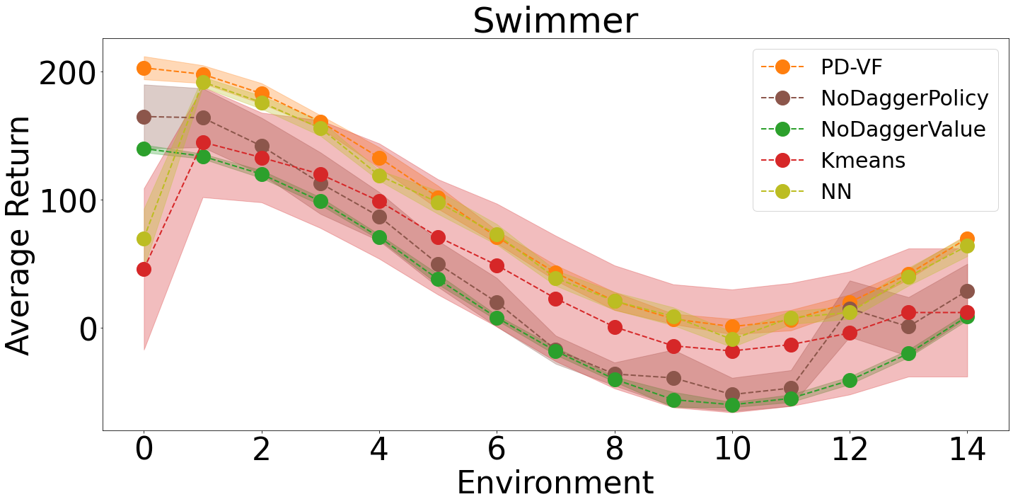
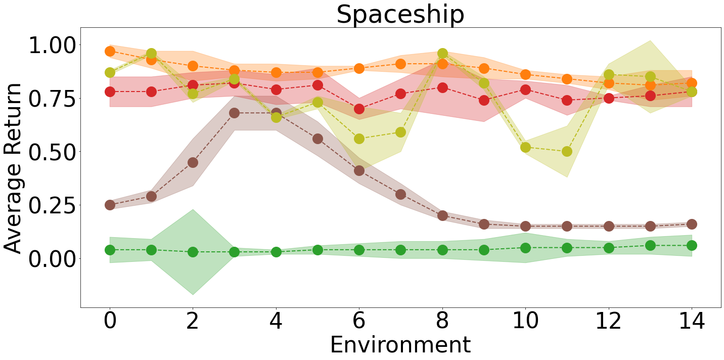
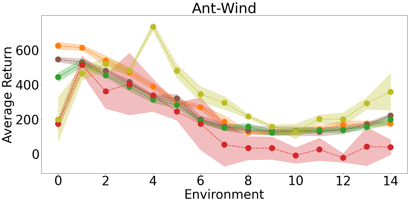
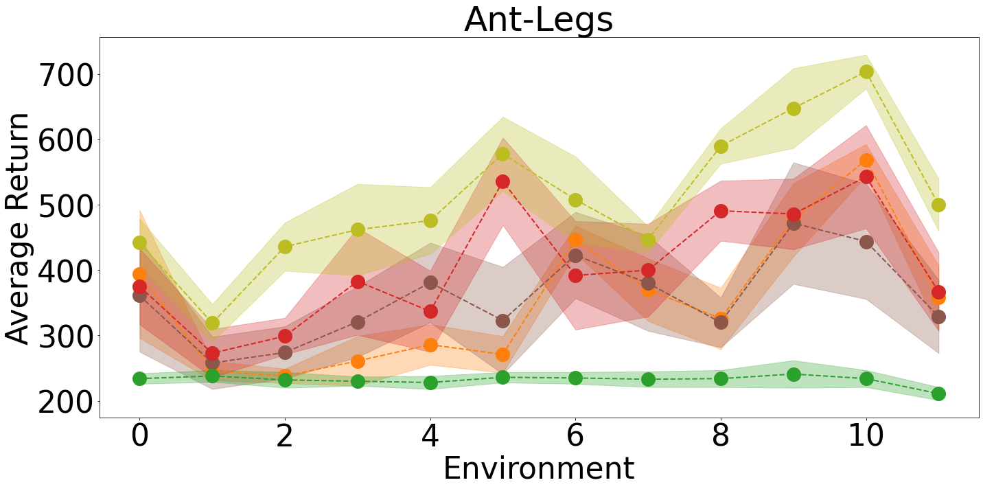
Figure 9: Train Performance. Average return on train environments in Swimmer (top-left), Spaceship (top-right), Ant-wind (bottom-left), and Ant-legs (bottom-right) obtained by PD-VF and a few ablations, namely NoDaggerPolicy, NoDaggerValue, Kmeans, and NN. PD-VF is comparable with or outperforms the ablations on the train environments. While some of these ablations perform reasonably well on the environments they are trained on, they generalize poorly to unseen dynamics.

Appendix F Analysis of Learned Embeddings

Figure 11 shows a t-SNE plot of the learned policy embeddings for Spaceship, Swimmer, and Ant (from left to right). The top and bottom rows color the embeddings by the policy and environment that generated the corresponding trajectory, respectively. Trajectories produced by the same policy have similar embeddings, while those generated in the same environment are not necessarily close in this embedding space. This shows that the policy embedding preserves information about the policy while disregarding elements of the environment (that generated the corresponding embedded trajectory).

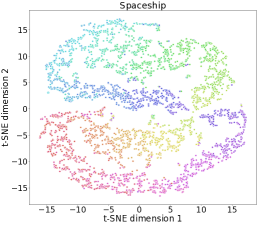
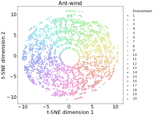
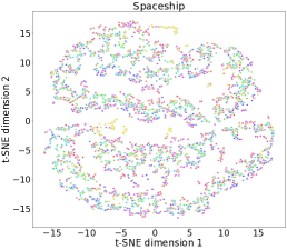
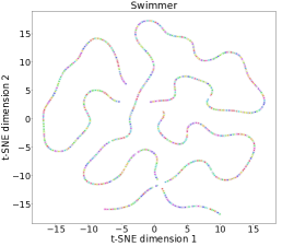
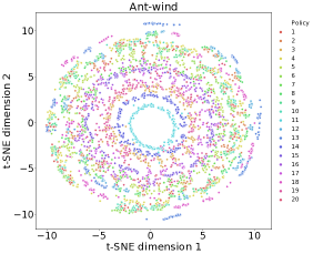
Figure 10: t-SNE plots of the learned environment embeddings $z_{d}$ for Spaceship, Swimmer, and Ant-wind (from left to right). The points are colored by the environment (top) and policy (bottom) used to generate the trajectory of the corresponding dynamics embedding.

Similarly, Figure 10 shows a t-SNE plot of the learned dynamics embeddings on the three continuous control domains used for evaluating our method. The top row colors each point by the corresponding environment used to generate the trajectory (from which the embedding is inferred), while the bottom row colors each point by the corresponding policy. One can see that the embedding space retrieves the true dynamics distribution and preserves the smoothness of the 1D manifold.

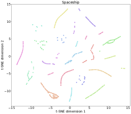
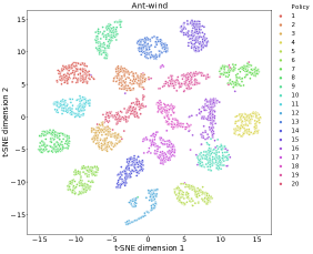
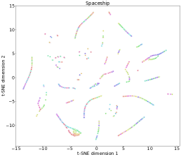
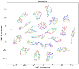
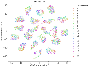
Figure 11: t-SNE plots of the learned policy embeddings $z_{\pi}$ for Spaceship, Swimmer, and Ant-wind (from left to right). The points are colored by the policy (top) and environment (bottom) used to generate the trajectory of the corresponding policy embedding.

Importantly, this analysis shows that the learned policy and dynamics embeddings are generally disentangled (i.e. information about the dynamics is not contained in the policy space and vice versa). This is important as we want the dynamics space to mostly capture information about the transition function and similarly, we want the policy space to capture variation in the agent behavior. The only exception is the dynamics space of Ant-wind, which contains information about both the environment and the policy. This is because in this environment, the policy is dominated by the force applied to the body of the ant, whose goal is to move forward (while incurring a penalty proportional to the applied force). Thus, depending on the wind direction in the training environment, the agent learns to apply a force of a certain magnitude, a characteristic captured in the embedding space. When evaluated on environments with different dynamics, that policy will still apply a similar force. Our experiments indicate that even if the dynamics space is not fully disentangled (yet it contains information about the environment), the PD-VF is still able to make effective use of the embeddings to find good policies for unseen environments and even outperform other state-of-the-art RL methods.

Appendix G The Challenge of Transfer

In this section, we emphasize the fact that the family of environments we designed pose a significant challenge to current state-of-the-art RL methods. To do this, we train PPO policies on each of the environments in our set (until convergence) and evaluate them on all other environments. The results show that any of the policies trained in this way can drastically fail in other environments (with different dynamics) from our training and test sets. This demonstrates that our set of environments provides a wide range of dynamics and that a single policy trained in any of these environments does not generalize well to the other ones. Moreover, when evaluated on a single environments, the performance across the pretrained policies varies greatly, illustrating the diversity of collected behaviors (both optimal and suboptimal). This analysis further supports the need for learning about multiple policies (and their performance in various environments) in order to generalize across widely different scenarios (or dynamics in this case).

	E1	E2	E3	E4	E5	E6	E7	E8	E9	E10
P1	598	354	128	372	291	95.9	-51.8	-50.9	-246	-299
P2	512	461	503	349	228	135	-1.44	-46.8	-28.1	-271
P3	689	620	593	500	334	80	0.4	-152	-51	-258
P4	654	665	557	519	29.9	180	177	-9.41	-90.5	-218.5
P5	935	962	947	930	853	648	429	287	155	-52.9
P6	811	838	794	778	710	600	386	247	123	-5.14
P7	624	659	408	451	351	474	394	82.9	151	55.9
P8	500	470	442	393	321	468	410	315	209	124
P9	303	326	297	295	265	254	243	238	11.1	223
P10	293	54.8	294	293	250	226	200	200	180	-1.28
P11	473	236	212	218	243	144	83.9	132	107	136
P12	266	264	268	242	214	181	55.6	72.7	239.4	240
P13	422	669	612	527	401	270	205	128	68.5	103
P14	436	362	424	366	259	296	97.3	55.7	24.9	-2.44
P15	420	484	264	125	131	66.7	44.5	13.1	5.43	35.1
P16	671	769	573	270	189	212	153	96.4	19.7	0.290
P17	784	793	683	600	56.9	200	56.8	12.4	4.4	19.8
P18	755	703	564	213	170	129	58.1	2.17	-103	-43.7
P19	182	593	415	65.5	250	112	25.8	37.1	-94.9	-19.2
P20	297	589	518	350	134	76.3	6.55	-51.5	-185.4	-11.2

Table 1: Performance of PPO policies on the Ant-wind domain. A row shows the mean episode return of a single policy on all environments, while a column shows the mean episode return of all policies on a single environment. This table contains performance on the first 10 environments.

	E11	E12	E13	E14	E15	E16	E17	E18	E19	E20
P1	-336	-136	-55.2	-7.47	-8.11	168	262	473	498	603
P2	-42.2	-101	-28.3	-112	14.2	132	109	345	510	545
P3	-54.1	-10.1	-232	-6.25	59.9	120	207	136	563	372
P4	-279	-278	-135	-4.81	5.49	113	276	150	484	196
P5	-264	-236	-69.8	14.0	77.6	248	457	602	813	634
P6	20.9	-112	98.7	147	14.9	194	321	524	611	639
P7	0.700	-5.74	-61.6	9.51	89.0	267	212	412	579	536
P8	39.6	-33.5	11.7	53.9	21.5	206	218	29.9	469	509
P9	7.05	216	225	224	248	253	284	266	314	281
P10	176	-159	5.98	5.03	57.8	20.6	77.0	287	249	539
P11	92.8	148	206	244	277	351	280	485	556	582
P12	235	235	232	122	139	151	165	299	272	265
P13	84.6	171	230	285	312	300	328	523	640	504
P14	45.2	159	126	302	369	363	537	457	512	396
P15	-4.98	-70.8	41.3	360	571	654	687	546	393	537
P16	-7.77	19.7	63.4	248	457	600	740	493	731	804
P17	-20.0	-102	-8.87	69.8	254	444	515	658	749	703
P18	-93.7	-59.9	-11.6	125	275	434	577	679	781	781
P19	-10.1	-16.9	1.38	18.6	86.5	126	372	508	489	652
P20	-118	-62.4	-125	-81.7	20.1	82.9	131	195	341	392

Table 2: Performance of PPO policies on the Ant-wind domain. A row shows the mean episode return of a single policy on all environments, while a column shows the mean episode return of all policies on a single environment. This table contains performance on the last 10 environments.

	E1	E2	E3	E4	E5	E6	E7	E8	E9	E10
P1	139.17	133.61	119.29	96.78	69.8	38.3	7.88	-19.59	-41.18	-54.88
P2	197.01	191.23	176.68	154.75	125.97	95.2	64.06	36.33	13.79	-1.1
P3	140.38	135.81	122.1	100.15	72.56	41.97	11.69	-15.47	-37.79	-51.59
P4	139.01	134.82	121.15	98.86	71.07	41.13	10.26	-17.24	-39.25	-54.68
P5	215.38	209.66	196.33	174.77	147.62	115.54	84.68	59.61	36.2	22.31
P6	207.08	201.55	186.96	165.49	138.86	107.64	77.12	49.94	28.6	14.55
P7	210.29	205.73	191.61	169.42	141.29	112.15	81.69	53.65	32.87	18.08
P8	213.98	209.7	198.61	179.11	152.56	124.49	95.18	67.78	45.47	32.82
P9	206.51	201.71	190.56	170.55	142.16	114.04	84.64	56.6	33.8	19.84
P10	204.85	201.04	186.64	168.29	141.0	113.45	80.69	53.39	33.46	19.9
P11	197.34	193.67	182.94	164.05	137.93	109.44	80.39	52.76	32.46	18.77
P12	204.92	201.11	186.85	166.49	138.03	108.22	79.32	50.95	29.97	16.23
P13	202.86	204.16	174.7	174.07	139.94	130.12	88.65	45.72	24.26	15.94
P14	205.89	201.64	187.07	166.63	138.54	108.87	77.48	51.66	29.76	15.68
P15	209.19	186.31	190.71	168.87	142.23	114.88	82.87	56.37	35.82	20.97
P16	214.29	204.26	188.0	165.51	140.3	109.66	80.35	56.25	37.05	23.41
P17	202.78	197.79	183.82	160.93	133.64	103.02	71.89	44.94	22.01	9.32
P18	202.66	204.15	190.16	167.73	139.81	109.03	77.82	51.18	29.4	14.83
P19	208.89	204.35	191.05	168.31	139.9	109.16	79.06	51.99	28.93	14.33
P20	141.37	136.28	122.22	100.69	73.13	42.51	12.4	-15.19	-37.6	-51.74

Table 3: Performance of PPO policies on the Swimmer domain. A row shows the mean episode return of a single policy on all environments, while a column shows the mean episode return of all policies on a single environment. This table contains performance on the first 10 environments.

	E11	E12	E13	E14	E15	E16	E17	E18	E19	E20
P1	-59.39	-54.24	-40.67	-19.18	9.2	39.2	69.81	97.3	119.73	134.49
P2	-6.11	-0.47	13.55	36.02	65.06	96.16	126.34	154.61	177.55	191.34
P3	-57.27	-52.51	-39.14	-16.39	10.56	40.38	71.77	98.78	121.09	135.31
P4	-58.16	-53.38	-39.35	-18.19	9.62	40.21	70.66	98.47	120.61	134.47
P5	16.13	20.32	32.89	56.59	85.07	114.87	144.05	173.91	196.76	210.27
P6	9.8	13.8	27.56	49.58	76.67	107.47	137.03	164.94	188.26	201.71
P7	14.63	19.66	34.54	56.04	82.39	114.16	143.69	171.16	190.65	205.65
P8	25.48	33.05	45.05	68.32	94.65	124.24	153.37	179.63	199.71	210.72
P9	15.39	19.33	31.88	54.41	79.43	110.51	139.44	165.05	186.49	200.29
P10	12.91	16.72	32.59	52.4	79.08	107.42	138.15	161.44	184.87	199.23
P11	12.84	17.28	30.41	50.77	76.78	104.17	132.33	156.83	178.78	191.66
P12	11.56	16.06	29.37	51.48	78.29	108.94	136.79	164.79	187.09	201.86
P13	3.07	-8.63	30.02	59.98	72.13	110.56	128.87	148.73	173.19	192.25
P14	10.65	16.23	30.17	52.24	79.07	109.76	139.88	166.59	187.43	202.78
P15	14.82	21.48	35.28	57.38	82.5	114.19	144.17	169.13	190.07	203.95
P16	18.92	23.92	36.31	57.05	88.57	116.78	147.6	172.97	196.18	209.08
P17	4.5	9.35	23.38	45.9	72.68	103.65	133.52	161.88	183.18	197.69
P18	10.91	14.36	29.04	49.94	78.39	109.27	140.76	167.58	189.9	202.89
P19	9.76	14.41	27.79	49.65	76.61	109.48	140.12	167.97	188.71	203.91
P20	-56.61	-52.49	-38.36	-16.25	11.95	42.14	72.88	100.43	122.74	136.87

Table 4: Performance of PPO policies on the Swimmer domain. A row shows the mean episode return of a single policy on all environments, while a column shows the mean episode return of all policies on a single environment. This table contains performance on the last 10 environments.

	E1	E2	E3	E4	E5	E6	E7	E8	E9	E10
P1	0.00	0.00	0.00	0.00	0.00	0.00	0.00	0.00	0.00	0.00
P2	0.97	0.97	0.92	0.92	0.90	0.91	0.93	0.95	0.99	0.95
P3	0.97	0.92	0.85	0.85	0.86	0.86	0.86	0.91	0.94	0.94
P4	0.00	0.00	0.00	0.00	0.00	0.00	0.00	0.00	0.00	0.00
P5	0.61	0.61	0.60	0.58	0.57	0.55	0.53	0.51	0.50	0.49
P6	0.96	0.90	0.87	0.87	0.88	0.90	0.91	0.92	0.96	0.95
P7	0.83	0.89	0.93	0.96	0.97	0.96	0.94	0.89	0.84	0.80
P8	0.84	0.84	0.84	0.82	0.81	0.79	0.78	0.77	0.75	0.74
P9	0.97	0.93	0.90	0.87	0.86	0.86	0.87	0.87	0.87	0.86
P10	0.91	0.90	0.88	0.87	0.87	0.88	0.89	0.92	0.96	0.98
P11	0.77	0.78	0.79	0.80	0.82	0.78	0.72	0.76	0.79	0.80
P12	0.67	0.56	0.39	0.46	0.58	0.41	0.39	0.46	0.49	0.47
P13	0.38	0.36	0.32	0.26	0.30	0.25	0.32	0.32	0.33	0.40
P14	0.82	0.79	0.76	0.74	0.73	0.72	0.72	0.73	0.75	0.76
P15	0.67	0.66	0.65	0.63	0.62	0.62	0.61	0.61	0.61	0.61
P16	0.00	0.00	0.00	0.00	0.00	0.00	0.00	0.00	0.00	0.00
P17	0.86	0.82	0.80	0.78	0.77	0.78	0.79	0.82	0.85	0.87
P18	0.69	0.68	0.66	0.65	0.64	0.63	0.63	0.63	0.63	0.63
P19	0.80	0.81	0.81	0.73	0.75	0.78	0.81	0.79	0.78	0.90
P20	0.96	0.94	0.90	0.88	0.87	0.86	0.86	0.86	0.85	0.83

Table 5: Performance of PPO policies on the Spaceship domain. A row shows the mean episode return of a single policy on all environments, while a column shows the mean episode return of all policies on a single environment. This table contains performance on the first 10 environments.

	E11	E12	E13	E14	E15	E16	E17	E18	E19	E20
P1	0.00	0.00	0.00	0.00	0.00	0.00	0.00	0.00	0.00	0.00
P2	0.89	0.85	0.82	0.79	0.79	0.79	0.81	0.84	0.87	0.92
P3	0.93	0.91	0.86	0.83	0.82	0.82	0.84	0.86	0.91	0.95
P4	0.00	0.00	0.00	0.00	0.00	0.00	0.00	0.00	0.00	0.00
P5	0.49	0.49	0.49	0.50	0.51	0.53	0.55	0.57	0.59	0.61
P6	0.91	0.85	0.82	0.79	0.78	0.78	0.80	0.82	0.86	0.92
P7	0.74	0.70	0.67	0.65	0.64	0.65	0.66	0.70	0.75	0.79
P8	0.73	0.71	0.70	0.70	0.70	0.71	0.73	0.76	0.79	0.82
P9	0.84	0.82	0.80	0.79	0.80	0.81	0.84	0.87	0.93	0.97
P10	0.94	0.90	0.86	0.84	0.83	0.83	0.85	0.88	0.90	0.92
P11	0.81	0.93	0.90	0.87	0.84	0.82	0.80	0.78	0.77	0.77
P12	0.46	0.83	0.61	0.44	0.77	0.74	0.64	0.59	0.59	0.63
P13	0.43	0.73	0.64	0.81	0.67	0.69	0.80	0.63	0.51	0.41
P14	0.79	0.80	0.82	0.85	0.86	0.89	0.91	0.91	0.89	0.85
P15	0.61	0.62	0.62	0.63	0.64	0.65	0.66	0.67	0.68	0.68
P16	0.00	0.00	0.00	0.00	0.00	0.00	0.00	0.00	0.00	0.00
P17	0.90	0.91	0.92	0.93	0.94	0.96	0.98	0.98	0.94	0.90
P18	0.63	0.63	0.64	0.64	0.65	0.67	0.68	0.69	0.70	0.70
P19	0.91	0.89	0.87	0.93	0.89	0.86	0.83	0.81	0.80	0.80
P20	0.80	0.78	0.77	0.76	0.76	0.77	0.80	0.85	0.90	0.93

Table 6: Performance of PPO policies on the Spaceship domain. A row shows the mean episode return of a single policy on all environments, while a column shows the mean episode return of all policies on a single environment. This table contains performance on the last 10 environments.

References

- Ammar et al. (2012) Ammar, H. B., Tuyls, K., Taylor, M. E., Driessens, K., and Weiss, G. Reinforcement learning transfer via sparse coding. In Proceedings of the 11th international conference on autonomous agents and multiagent systems, volume 1, pp. 383–390. International Foundation for Autonomous Agents and Multiagent Systems …, 2012.
- Ammar et al. (2014) Ammar, H. B., Eaton, E., Taylor, M. E., Mocanu, D. C., Driessens, K., Weiss, G., and Tuyls, K. An automated measure of mdp similarity for transfer in reinforcement learning. In Workshops at the Twenty-Eighth AAAI Conference on Artificial Intelligence, 2014.
- Andreas et al. (2017) Andreas, J., Klein, D., and Levine, S. Modular multitask reinforcement learning with policy sketches. In International Conference on Machine Learning, pp. 166–175, 2017.
- Arnekvist et al. (2018) Arnekvist, I., Kragic, D., and Stork, J. A. Vpe: Variational policy embedding for transfer reinforcement learning. 2019 International Conference on Robotics and Automation (ICRA), pp. 36–42, 2018.
- Barreto et al. (2017) Barreto, A., Dabney, W., Munos, R., Hunt, J. J., Schaul, T., van Hasselt, H. P., and Silver, D. Successor features for transfer in reinforcement learning. In Advances in neural information processing systems, pp. 4055–4065, 2017.
- Berner et al. (2019) Berner, C., Brockman, G., Chan, B., Cheung, V., Debiak, P., Dennison, C., Farhi, D., Fischer, Q., Hashme, S., Hesse, C., Józefowicz, R., Gray, S., Olsson, C., Pachocki, J. W., Petrov, M., de Oliveira Pinto, H. P., Raiman, J., Salimans, T., Schlatter, J., Schneider, J., Sidor, S., Sutskever, I., Tang, J., Wolski, F., and Zhang, S. Dota 2 with large scale deep reinforcement learning. ArXiv, abs/1912.06680, 2019.
- Borsa et al. (2016) Borsa, D., Graepel, T., and Shawe-Taylor, J. Learning shared representations in multi-task reinforcement learning. arXiv preprint arXiv:1603.02041, 2016.
- Borsa et al. (2018) Borsa, D., Barreto, A., Quan, J., Mankowitz, D., Munos, R., van Hasselt, H., Silver, D., and Schaul, T. Universal successor features approximators. arXiv preprint arXiv:1812.07626, 2018.
- Co-Reyes et al. (2018) Co-Reyes, J. D., Liu, Y., Gupta, A., Eysenbach, B., Abbeel, P., and Levine, S. Self-consistent trajectory autoencoder: Hierarchical reinforcement learning with trajectory embeddings. In ICML, 2018.
- Cobbe et al. (2019) Cobbe, K., Klimov, O., Hesse, C., Kim, T., and Schulman, J. Quantifying generalization in reinforcement learning. In ICML, 2019.
- Cully et al. (2015) Cully, A., Clune, J., Tarapore, D., and Mouret, J.-B. Robots that can adapt like animals. Nature, 521:503–507, 2015.
- Da Silva et al. (2012) Da Silva, B., Konidaris, G., and Barto, A. Learning parameterized skills. arXiv preprint arXiv:1206.6398, 2012.
- Devin et al. (2016) Devin, C., Gupta, A., Darrell, T., Abbeel, P., and Levine, S. Learning modular neural network policies for multi-task and multi-robot transfer. 2017 IEEE International Conference on Robotics and Automation (ICRA), pp. 2169–2176, 2016.
- Doshi-Velez & Konidaris (2013) Doshi-Velez, F. and Konidaris, G. Hidden parameter markov decision processes: A semiparametric regression approach for discovering latent task parametrizations. IJCAI : proceedings of the conference, 2016:1432–1440, 2013.
- Duan et al. (2016) Duan, Y., Schulman, J., Chen, X., Bartlett, P. L., Sutskever, I., and Abbeel, P. Rl2: Fast reinforcement learning via slow reinforcement learning. ArXiv, abs/1611.02779, 2016.
- Duan et al. (2017) Duan, Y., Andrychowicz, M., Stadie, B. C., Ho, J., Schneider, J., Sutskever, I., Abbeel, P., and Zaremba, W. One-shot imitation learning. In NIPS, 2017.
- Finn et al. (2017) Finn, C., Abbeel, P., and Levine, S. Model-agnostic meta-learning for fast adaptation of deep networks. In Proceedings of the 34th International Conference on Machine Learning-Volume 70, pp. 1126–1135. JMLR. org, 2017.
- Gupta et al. (2017) Gupta, A., Devin, C., Liu, Y., Abbeel, P., and Levine, S. Learning invariant feature spaces to transfer skills with reinforcement learning. arXiv preprint arXiv:1703.02949, 2017.
- Hansen et al. (2019) Hansen, S., Dabney, W., Barreto, A., Van de Wiele, T., Warde-Farley, D., and Mnih, V. Fast task inference with variational intrinsic successor features. arXiv preprint arXiv:1906.05030, 2019.
- Hausman et al. (2018) Hausman, K., Springenberg, J. T., Wang, Z., Heess, N. M. O., and Riedmiller, M. A. Learning an embedding space for transferable robot skills. In ICLR, 2018.
- He et al. (2018) He, Z., Julian, R., Heiden, E., Zhang, H., Schaal, S., Lim, J. J., Sukhatme, G., and Hausman, K. Zero-shot skill composition and simulation-to-real transfer by learning task representations. arXiv preprint arXiv:1810.02422, 2018.
- Henderson et al. (2018) Henderson, P., Islam, R., Bachman, P., Pineau, J., Precup, D., and Meger, D. Deep reinforcement learning that matters. In Thirty-Second AAAI Conference on Artificial Intelligence, 2018.
- Hessel et al. (2019) Hessel, M., Soyer, H., Espeholt, L., Czarnecki, W., Schmitt, S., and van Hasselt, H. Multi-task deep reinforcement learning with popart. In Proceedings of the AAAI Conference on Artificial Intelligence, volume 33, pp. 3796–3803, 2019.
- Higgins et al. (2017) Higgins, I., Pal, A., Rusu, A. A., Matthey, L., Burgess, C., Pritzel, A., Botvinick, M. M., Blundell, C., and Lerchner, A. Darla: Improving zero-shot transfer in reinforcement learning. In ICML, 2017.
- Houthooft et al. (2018) Houthooft, R., Chen, R. Y., Isola, P., Stadie, B. C., Wolski, F., Ho, J., and Abbeel, P. Evolved policy gradients. ArXiv, abs/1802.04821, 2018.
- Humplik et al. (2019) Humplik, J., Galashov, A., Hasenclever, L., Ortega, P. A., Teh, Y. W., and Heess, N. Meta reinforcement learning as task inference. arXiv preprint arXiv:1905.06424, 2019.
- Jaderberg et al. (2019) Jaderberg, M., Czarnecki, W. M., Dunning, I., Marris, L., Lever, G., Castaneda, A. G., Beattie, C., Rabinowitz, N. C., Morcos, A. S., Ruderman, A., et al. Human-level performance in 3d multiplayer games with population-based reinforcement learning. Science, 364(6443):859–865, 2019.
- Killian et al. (2017) Killian, T. W., Konidaris, G., and Doshi-Velez, F. Robust and efficient transfer learning with hidden parameter markov decision processes. Advances in neural information processing systems, 30:6250–6261, 2017.
- Kingma & Ba (2014) Kingma, D. P. and Ba, J. Adam: A method for stochastic optimization. arXiv preprint arXiv:1412.6980, 2014.
- Kingma & Welling (2013) Kingma, D. P. and Welling, M. Auto-encoding variational bayes. CoRR, abs/1312.6114, 2013.
- Lazaric (2012) Lazaric, A. Transfer in reinforcement learning: a framework and a survey. In Reinforcement Learning, pp. 143–173. Springer, 2012.
- Madjiheurem & Toni (2019) Madjiheurem, S. and Toni, L. State2vec: Off-policy successor features approximators. arXiv preprint arXiv:1910.10277, 2019.
- Mnih et al. (2015) Mnih, V., Kavukcuoglu, K., Silver, D., Rusu, A. A., Veness, J., Bellemare, M. G., Graves, A., Riedmiller, M., Fidjeland, A. K., Ostrovski, G., et al. Human-level control through deep reinforcement learning. Nature, 518(7540):529–533, 2015.
- Nagabandi et al. (2018) Nagabandi, A., Clavera, I., Liu, S., Fearing, R. S., Abbeel, P., Levine, S., and Finn, C. Learning to adapt in dynamic, real-world environments through meta-reinforcement learning. arXiv preprint arXiv:1803.11347, 2018.
- Oh et al. (2017) Oh, J., Singh, S., Lee, H., and Kohli, P. Zero-shot task generalization with multi-task deep reinforcement learning. arXiv preprint arXiv:1706.05064, 2017.
- Parisotto et al. (2015) Parisotto, E., Ba, J. L., and Salakhutdinov, R. Actor-mimic: Deep multitask and transfer reinforcement learning. arXiv preprint arXiv:1511.06342, 2015.
- Paul et al. (2018) Paul, S., Osborne, M. A., and Whiteson, S. Fingerprint policy optimisation for robust reinforcement learning. In ICML, 2018.
- Perez et al. (2018) Perez, C. F., Such, F. P., and Karaletsos, T. Efficient transfer learning and online adaptation with latent variable models for continuous control. ArXiv, abs/1812.03399, 2018.
- Petangoda et al. (2019) Petangoda, J. C., Pascual-Diaz, S., Adam, V., Vrancx, P., and Grau-Moya, J. Disentangled skill embeddings for reinforcement learning. ArXiv, abs/1906.09223, 2019.
- Pinto et al. (2017) Pinto, L., Davidson, J., Sukthankar, R., and Gupta, A. Robust adversarial reinforcement learning. In ICML, 2017.
- Precup et al. (2001) Precup, D., Sutton, R. S., and Dasgupta, S. Off-policy temporal-difference learning with function approximation. In ICML, pp. 417–424, 2001.
- Raileanu & Rocktäschel (2020) Raileanu, R. and Rocktäschel, T. Ride: Rewarding impact-driven exploration for procedurally-generated environments. ArXiv, abs/2002.12292, 2020.
- Rajeswaran et al. (2017) Rajeswaran, A., Lowrey, K., Todorov, E. V., and Kakade, S. M. Towards generalization and simplicity in continuous control. In Advances in Neural Information Processing Systems, pp. 6550–6561, 2017.
- Rakelly et al. (2019) Rakelly, K., Zhou, A., Finn, C., Levine, S., and Quillen, D. Efficient off-policy meta-reinforcement learning via probabilistic context variables. In International conference on machine learning, pp. 5331–5340, 2019.
- Sæmundsson et al. (2018) Sæmundsson, S., Hofmann, K., and Deisenroth, M. P. Meta reinforcement learning with latent variable gaussian processes. arXiv preprint arXiv:1803.07551, 2018.
- Sahni et al. (2017) Sahni, H., Kumar, S., Tejani, F., and Isbell, C. Learning to compose skills. arXiv preprint arXiv:1711.11289, 2017.
- Schaul et al. (2015) Schaul, T., Horgan, D., Gregor, K., and Silver, D. Universal value function approximators. In International conference on machine learning, pp. 1312–1320, 2015.
- Schulman et al. (2017) Schulman, J., Wolski, F., Dhariwal, P., Radford, A., and Klimov, O. Proximal policy optimization algorithms. arXiv preprint arXiv:1707.06347, 2017.
- Silver et al. (2016) Silver, D., Huang, A., Maddison, C. J., Guez, A., Sifre, L., Van Den Driessche, G., Schrittwieser, J., Antonoglou, I., Panneershelvam, V., Lanctot, M., et al. Mastering the game of go with deep neural networks and tree search. nature, 529(7587):484, 2016.
- Silver et al. (2017) Silver, D., Schrittwieser, J., Simonyan, K., Antonoglou, I., Huang, A., Guez, A., Hubert, T., Baker, L., Lai, M., Bolton, A., et al. Mastering the game of go without human knowledge. nature, 550(7676):354–359, 2017.
- Silver et al. (2018) Silver, D., Hubert, T., Schrittwieser, J., Antonoglou, I., Lai, M., Guez, A., Lanctot, M., Sifre, L., Kumaran, D., Graepel, T., et al. A general reinforcement learning algorithm that masters chess, shogi, and go through self-play. Science, 362(6419):1140–1144, 2018.
- Siriwardhana et al. (2019) Siriwardhana, S., Weerasakera, R., Matthies, D. J., and Nanayakkara, S. Vusfa: Variational universal successor features approximator to improve transfer drl for target driven visual navigation. arXiv preprint arXiv:1908.06376, 2019.
- Song et al. (2020) Song, X., Jiang, Y., Tu, S., Du, Y., and Neyshabur, B. Observational overfitting in reinforcement learning. ArXiv, abs/1912.02975, 2020.
- Sutton et al. (2011) Sutton, R. S., Modayil, J., Delp, M., Degris, T., Pilarski, P. M., White, A., and Precup, D. Horde: a scalable real-time architecture for learning knowledge from unsupervised sensorimotor interaction. In AAMAS, 2011.
- Taylor & Stone (2009) Taylor, M. E. and Stone, P. Transfer learning for reinforcement learning domains: A survey. Journal of Machine Learning Research, 10(Jul):1633–1685, 2009.
- Teh et al. (2017) Teh, Y., Bapst, V., Czarnecki, W. M., Quan, J., Kirkpatrick, J., Hadsell, R., Heess, N., and Pascanu, R. Distral: Robust multitask reinforcement learning. In Advances in Neural Information Processing Systems, pp. 4496–4506, 2017.
- Todorov et al. (2012) Todorov, E., Erez, T., and Tassa, Y. Mujoco: A physics engine for model-based control. 2012 IEEE/RSJ International Conference on Intelligent Robots and Systems, pp. 5026–5033, 2012.
- van der Maaten & Hinton (2008) van der Maaten, L. and Hinton, G. E. Visualizing data using t-sne. 2008.
- Vaswani et al. (2017) Vaswani, A., Shazeer, N., Parmar, N., Uszkoreit, J., Jones, L., Gomez, A. N., Kaiser, Ł., and Polosukhin, I. Attention is all you need. In Advances in neural information processing systems, pp. 5998–6008, 2017.
- Vinyals et al. (2019) Vinyals, O., Babuschkin, I., Czarnecki, W. M., Mathieu, M., Dudzik, A., Chung, J., Choi, D. H., Powell, R., Ewalds, T., Georgiev, P., et al. Grandmaster level in starcraft ii using multi-agent reinforcement learning. Nature, 575(7782):350–354, 2019.
- Wang et al. (2016) Wang, J. X., Kurth-Nelson, Z., Soyer, H., Leibo, J. Z., Tirumala, D., Munos, R., Blundell, C., Kumaran, D., and Botvinick, M. M. Learning to reinforcement learn. ArXiv, abs/1611.05763, 2016.
- Wang et al. (2017) Wang, Z., Merel, J., Reed, S. E., de Freitas, N., Wayne, G., and Heess, N. M. O. Robust imitation of diverse behaviors. In NIPS, 2017.
- White et al. (2012) White, A., Modayil, J., and Sutton, R. S. Scaling life-long off-policy learning. In 2012 IEEE International Conference on Development and Learning and Epigenetic Robotics (ICDL), pp. 1–6. IEEE, 2012.
- Whiteson et al. (2011) Whiteson, S., Tanner, B., Taylor, M. E., and Stone, P. Protecting against evaluation overfitting in empirical reinforcement learning. 2011 IEEE Symposium on Adaptive Dynamic Programming and Reinforcement Learning (ADPRL), pp. 120–127, 2011.
- Xu et al. (2018) Xu, Z., van Hasselt, H., and Silver, D. Meta-gradient reinforcement learning. In NeurIPS, 2018.
- Yang et al. (2019) Yang, J., Petersen, B., Zha, H., and Faissol, D. Single episode policy transfer in reinforcement learning. arXiv preprint arXiv:1910.07719, 2019.
- Yao et al. (2018) Yao, J., Killian, T. W., Konidaris, G., and Doshi-Velez, F. Direct policy transfer via hidden parameter markov decision processes. 2018.
- Zhang et al. (2018a) Zhang, A., Ballas, N., and Pineau, J. A dissection of overfitting and generalization in continuous reinforcement learning. arXiv preprint arXiv:1806.07937, 2018a.
- Zhang et al. (2018b) Zhang, A., Satija, H., and Pineau, J. Decoupling dynamics and reward for transfer learning. ArXiv, abs/1804.10689, 2018b.
- Zhang et al. (2018c) Zhang, C., Vinyals, O., Munos, R., and Bengio, S. A study on overfitting in deep reinforcement learning. arXiv preprint arXiv:1804.06893, 2018c.
- Zhang et al. (2017) Zhang, J., Springenberg, J. T., Boedecker, J., and Burgard, W. Deep reinforcement learning with successor features for navigation across similar environments. In 2017 IEEE/RSJ International Conference on Intelligent Robots and Systems (IROS), pp. 2371–2378. IEEE, 2017.
- Zintgraf et al. (2018) Zintgraf, L. M., Shiarlis, K., Kurin, V., Hofmann, K., and Whiteson, S. Fast context adaptation via meta-learning. In ICML, 2018.