Non-Markovianity of Quantum Brownian Motion

Abstract

We study quantum non-Markovian dynamics of the Caldeira-Leggett model, a prototypical model for quantum Brownian motion describing a harmonic oscillator linearly coupled to a reservoir of harmonic oscillators. Employing the exact analytical solution of this model one can determine the size of memory effects for arbitrary couplings, temperatures and frequency cutoffs. Here, quantum non-Markovianity is defined in terms of the flow of information between the open system and its environment, which is quantified through the Bures metric as distance measure for quantum states. This approach allows us to discuss quantum memory effects in the whole range from weak to strong dissipation for arbitrary Gaussian initial states. A comparison of our results with the corresponding results for the spin-boson problem show a remarkable similarity in the structure of non-Markovian behavior of the two paradigmatic models.

I Introduction

How do memory effects manifest themselves in the dynamics of open quantum systems Breuer and Petruccione (2002), what are the characteristic features of these effects and how can they be rigorously defined and quantified? These questions play an important role in many applications of quantum mechanics and have received a tremendous amount of interest in recent years (see, e.g., the reviews Rivas et al. (2014); Breuer et al. (2016); de Vega and Alonso (2017)). In fact, the problems of the mathematical definition and of the physical implications of quantum memory effects in open systems has initiated a large variety of interesting applications to diverse quantum systems and phenomena. Examples include Ising and Heisenberg spin chains and Bose-Einstein condensates Apollaro et al. (2011); Haikka et al. (2011, 2012), quantum phase transitions Gessner et al. (2014a), optomechanical systems Gröblacher et al. (2015), chaotic systems Znidaric et al. (2011); García-Mata et al. (2012), energy transfer processes in photosynthetic complexes Rebentrost and Aspuru-Guzik (2011), spectral line shapes and two-dimensional spectra Green et al. (2019), continuous variable quantum key distribution Vasile et al. (2011a), and quantum metrology Chin et al. (2012). Moreover, experimental realizations of quantum non-Markovianity and its control have been reported for both photonic and trapped ion systems Liu et al. (2011); Li et al. (2011); Smirne et al. (2011); Gessner et al. (2014b); Cialdi et al. (2014); Tang et al. (2015).

As shown in Ref. Breuer et al. (2009) a systematic approach to the theoretical description of memory effects of open systems can be based on concepts of quantum information theory. Within this approach memory effects are connected to the exchange of information between the open system and its environment. This means that Markovian, i.e. memoryless behaviour is characterized by a continuous loss of information, that is by a continuous flow of information from the open system to its surroundings, while non-Markovian dynamics is distinguished by a back flow of information from the environment to the open system. Employing the trace distance between quantum states as a measure for their distinguishably Helstrom (1976); Hayashi (2006) and, hence, as a measure for the amount of information inside the open system, Markovian quantum dynamics is characterized by a monotonic decrease of the trace distance, while non-Markovian dynamics features a non-monotonic behaviour of the trace distance for a pair of quantum states.

Here, we apply these concepts to the Caldeira-Leggett model of quantum Brownian motion Caldeira and Leggett (1983); Grabert et al. (1988). To this end, we study the integrable case of a harmonic oscillator, representing the open system, which is coupled to a harmonic oscillator reservoir, and perform a systematic analysis of the quantum non-Markovianity based on the concept of the information flow between open system and reservoir. However, for technical simplicity we follow the approach of Ref. Vasile et al. (2011b) and use, instead of the trace distance, the Bures metric Hayashi (2006) as distance measure for quantum states. This metric is defined by means of the fidelity of quantum states, it is closely related to the trace distance and has similar mathematical properties. In particular, trace preserving completely positive maps are contractions for the Bures metric, a property which is important for the definition of quantum non-Markovianity Laine et al. (2010). The advantage of this approach is that the Bures distance between two Gaussian states can easily be determined by means of an analytical expression, which enables an efficient calculation of the non-Markovianity in a wide range of system-reservoir coupling, reservoir temperatures and frequency cutoffs.

The paper is organized as follows. In Sec. II we briefly recall the concepts of information flow and non-Markovianity of the dynamics of open quantum systems. In particular, we discuss the treatment of arbitrary Gaussian initial states as well as the application of the general approach to the Caldeira-Leggett model. The simulation results are discussed in detail in Sec. III. In particular, we investigate the strong damping limit and compare our results with previous results obtained for the spin-boson model. Moreover, we examine the limiting case described by the Caldeira-Leggett master equation, and study also the case of an external driving of the system or the reservoir. Finally, in Sec. IV we summarise our results and draw our conclusions.

II Quantum information flow and memory effects

II.1 Non-Markovianity and Gaussian initial states

As mentioned in the Introduction we will use here the approach to quantum non-Markovianity proposed in Ref. Breuer et al. (2009) which is based on the trace distance between two quantum states $\rho_{1}$ and $\rho_{2}$ defined by

$$D(\rho_{1},\rho_{2})=\frac{1}{2}\operatorname{Tr}|\rho_{1}-\rho_{2}|,$$ (1)

where $|A|=\sqrt{A^{\dagger}A}$ denotes the modulus of an operator $A$. The time evolution of the states can be represented by a family of trace-preserving and completely positive (CP) quantum dynamical maps $\Phi_{t}$,

$$\Phi=\Big{\{}\Phi_{t}\mid\Phi_{0}={\rm id},\,t\in[0,t_{\rm max}]\Big{\}},$$ (2)

such that $\rho_{1,2}(t)=\Phi_{t}\rho_{1,2}(0)$ represent the states at time $t\in[0,t_{\rm max}]$. In view of the interpretation of the trace distance in terms of the distinguishability of the quantum states, a dynamical decrease of $D(\rho_{1}(t),\rho_{2}(t))$ can be interpreted as a loss of information from the open system into the environment characteristic of Markovian dynamics and, vice versa, any increase of $D(\rho_{1}(t),\rho_{2}(t))$ as a flow of information from the environment back to the system signifying memory effects and non-Markovian behavior. Since trace-preserving positive and completely positive maps are contractions for the trace distance, any P-divisible or CP-divisible dynamics Breuer et al. (2016) provides an example of a monotonically decreasing trace distance and, hence, of a Markovian dynamics Chruściński et al. (2011); Wißmann et al. (2015). In particular, any dynamics given by a semigroup with a generator in Lindblad form is Markovian according to this definition.

The degree of memory effects of a given dynamics can be quantified by integrating the total information backflow from the environment to the system leading to the non-Markoviantiy measure Breuer et al. (2009)

$$\mathcal{N}(\Phi)=\max_{\rho_{1,2}(0)}\int_{\sigma>0}\text{d}t\ \sigma(t),$$ (3)

where

$$\sigma(t)=\frac{d}{dt}D\big{(}\Phi_{t}\rho_{1}(0),\Phi_{t}\rho_{2}(0)\big{)},$$ (4)

and the integration is taken over all time intervals of the full interval $[0,t_{\rm max}]$ in which $\sigma(t)>0$.

In this paper we will investigate the time evolution of Gaussian initial states, which preserve their Gaussianity under the action of the time evolution operators generated by the quadratic Caldeira-Leggett Hamiltonian. As explained in the Introduction, instead of the trace distance we will consider here the Bures distance Hayashi (2006) of quantum states which leads to a simple expression for Gaussian states in terms of the first two moments of the position and momentum operators of the open system Vasile et al. (2011b). To this end, we introduce the quantum fidelity defined by

$$\mathcal{F}(\rho_{1},\rho_{2})=\left[\operatorname{Tr}\left\{\sqrt{\sqrt{\rho_{1}}\rho_{2}\sqrt{\rho_{1}}}\right\}\right]^{2},$$ (5)

which is equal to one if and only if $\rho_{1}=\rho_{2}$ and equal to zero if and only if $\rho_{1}$ and $\rho_{2}$ have orthogonal support. We introduce the dimensionless quadrature operators $X=(\hat{a}+\hat{a}^{\dagger})/\sqrt{2}$ and $P=i(\hat{a}^{\dagger}-\hat{a})/\sqrt{2}$, which we can arrange in the vector operator $\mathbf{R}=(X,P)^{T}$. The fidelity can then be expressed in terms of the first two moments of the two single mode Gaussian states $\rho_{1}$ and $\rho_{2}$ as

$$\mathcal{F}(\rho_{1},\rho_{2})=\frac{2}{\sqrt{\Delta+\delta}-\sqrt{\delta}}e^{-\frac{1}{2}(\mathbf{d}_{2}-\mathbf{d}_{1})^{T}(\bm{\sigma}_{1}+\bm{\sigma}_{2})^{-1}(\mathbf{d}_{2}-\mathbf{d}_{1})},$$ (6)

where

$$\Delta =4\det(\bm{\sigma}_{1}+\bm{\sigma}_{2}),$$ (7)

$$\delta =16\left[\det(\bm{\sigma}_{1})-\frac{1}{4}\right]\left[\det(\bm{\sigma}_{2})-\frac{1}{4}\right].$$ (8)

Here, $\bm{\sigma}_{1,2}$ are the covariance matrices of the states with the elements

$$(\bm{\sigma}_{1,2})_{ij}=\frac{1}{2}\langle\{R_{i},R_{j}\}\rangle_{\rho_{1,2}}-\langle R_{i}\rangle_{\rho_{1,2}}\langle R_{j}\rangle_{\rho_{1,2}}$$ (9)

and

$$\mathbf{d}_{1,2}=\langle\mathbf{R}\rangle_{\rho_{1,2}}$$ (10)

represent the mean values of the two states.

Now, the Bures distance is defined with help of the fidelity by means of

$$D_{B}(\rho_{1},\rho_{2})=\sqrt{2-2\sqrt{\mathcal{F}(\rho_{1},\rho_{2})}}.$$ (11)

We note that, like the trace distance, the Bures distance is contracting under any trace-preserving (completely) positive map. Moreover, the Bures distance and the trace distance are related by the inequalities Bengtsson and Zyczkowski (2006)

$$\sqrt{2-2\sqrt{1-D(\rho_{1},\rho_{2})^{2}}}\leq D_{B}(\rho_{1},\rho_{2})\leq\sqrt{2D(\rho_{1},\rho_{2})}.$$ (12)

The measure for non-Markovianity (3) involves a maximization over all pairs of initial states in order to make the expression a functional of the family $\Phi$ of dynamical maps given in Eq. (2). In the following we will omit this maximization and consider a fixed pair of initial states. The measure thus describes the degree of memory effects for the specific process defined by the dynamical map and a certain pair of initial conditions. Summarizing, in the following we will investigate the quantity

$$\mathcal{N}(\Phi)=\int_{\sigma>0}\text{d}t\ \sigma(t),$$ (13)

where

$$\sigma(t)=\frac{d}{dt}D_{B}\big{(}\rho_{1}(t),\rho_{2}(t)\big{)}.$$ (14)

II.2 Application to the Caldeira-Leggett model

The Caldeira-Leggett model describes an open quantum system linearly coupled via the position coordinate to an infinite bath of quantum harmonic oscillators. We assume that the open system also represents a harmonic oscillator such that the Hamiltonian is given by Caldeira and Leggett (1983)

$$H= \underbrace{\frac{1}{2m}p^{2}+\frac{1}{2}m\omega_{0}^{2}x^{2}}_{\text{$H_{S}$}}+\underbrace{\sum_{n}\left(\frac{1}{2m_{n}}p_{n}^{2}+\frac{1}{2}m_{n}\omega_{n}^{2}x_{n}^{2}\right)}_{\text{$H_{B}$}}$$

$$\underbrace{-x\sum_{n}\kappa_{n}x_{n}}_{\text{$H_{I}$}}+\underbrace{x^{2}\sum_{n}\frac{\kappa_{n}^{2}}{2m_{n}\omega_{n}^{2}}}_{\text{counterterm}}.$$ (15)

The coordinate and momentum operators of the central oscillator and the bath oscillators are $x$, $p$ and $x_{n}$, $p_{n}$, respectively. The first two terms $H_{S}$ and $H_{B}$ are the energy contributions of the open system and the bath oscillators, respectively. The third part is the interaction term between the system and the bath. The coupling strength between the system and the $j$-th bath oscillator is represented by $\kappa_{j}$. Furthermore a counter term is typically introduced in the Hamiltonian, which accounts for a renormalization of the central oscillator frequency due to the interaction with the bath Grabert et al. (1988).

The bath and interaction characteristics are fully described by the so-called spectral density

$$J(\omega)=\sum_{n}\frac{\kappa_{n}^{2}}{2m_{n}\omega_{n}}\delta(\omega-\omega_{n}).$$ (16)

In the limit of infinitely many bath oscillators the spectral density may be represented by a smooth function of frequency. In the following we choose an Ohmic spectral density with a Lorentz-Drude cutoff of the form

$$J(\omega)=\frac{2m\gamma}{\pi}\omega\ \frac{\Omega^{2}}{\Omega^{2}+\omega^{2}}.$$ (17)

We call $\gamma$ the coupling strength and $\Omega$ the frequency cutoff.

In order to calculate the time evolution of the Bures distance for Gaussian initial states we need to find the time evolution of the first two moments of the momentum and position operators of the open system. Those in turn can be calculated by finding the time evolution of the position and momentum operators in the Heisenberg picture. From the Heisenberg equation of motions of $x(t)$, $x_{n}(t)$, $p(t)$ and $p_{n}(t)$ generated by the total Caldeira-Leggett Hamiltonian it is possible to derive the following operator valued integro-differential equation for the position operator Breuer and Petruccione (2002)

$$\ddot{x}(t)+\omega_{0}^{2}x(t)+\frac{d}{dt}\int\limits_{0}^{t}dt^{\prime}\gamma(t-t^{\prime})x(t^{\prime})=\frac{1}{m}B(t),$$ (18)

where

$$B(t)=\sum_{n}\kappa_{n}\sqrt{\frac{1}{2m_{n}\omega_{n}}}\left(e^{-i\omega_{n}t}a_{n}+e^{+i\omega_{n}t}a_{n}^{\dagger}\right)$$ (19)

is the stochastic force and

$$\gamma(t)=\frac{2}{m}\int_{0}^{\infty}d\omega\frac{J(\omega)}{\omega}\cos(\omega t)$$ (20)

the damping kernel. This equation can be solved by Laplace transformation with the solution

$$x(t)=G_{1}(t)x(0)+G_{2}(t)\frac{p(0)}{m}+\frac{1}{m}\int\limits_{0}^{t}dt^{\prime}G_{2}(t-t^{\prime})B(t^{\prime}).$$ (21)

The solution for the time evolution of the momentum operator is determined by $p(t)=m\frac{d}{dt}x(t)$. The functions $G_{1}(t)$ and $G_{2}(t)$ are the solutions of the homogeneous part of Eq. (18) corresponding to the initial conditions $G_{1}(0)=1$, $\dot{G}_{1}(0)=0$ and $G_{2}(0)=0$, $\dot{G}_{2}(0)=1$, respectively. These Green’s functions can be obtained by Laplace transformation which yields

$$\hat{G}_{2}(z)=\frac{\hat{G}_{1}(z)}{z}=\frac{1}{z^{2}+z\hat{\gamma}(z)+\omega_{0}^{2}}.$$ (22)

The Laplace transform of the damping kernel corresponding to a Lorentz-Drude spectral density reads

$$\hat{\gamma}(z)=2\gamma\frac{\Omega}{z+\Omega}$$ (23)

and, hence, the Laplace transform of $G_{2}(t)$ is given in this case by

$$\hat{G}_{2}(z)=\frac{z+\Omega}{z^{3}+\Omega z^{2}+(\omega_{0}^{2}+2\gamma\Omega)z+\omega_{0}^{2}\Omega}.$$ (24)

With help of the residual theorem one performs the back transformation and arrives at

$$G_{2}(t)=\sum_{i=1}^{3}d_{i}e^{z_{i}t},$$ (25)

where $z_{i}$ are the poles of $\hat{G}_{2}(z)$ determined by the roots of the cubic polynomial in the denominator in Eq. (24),

$$z^{3}+\Omega z^{2}+(\omega_{0}^{2}+2\gamma\Omega)z+\omega_{0}^{2}\Omega=0.$$ (26)

The discriminant of this cubic equation in dependence on the coupling strength $\gamma$ and the frequency cutoff $\Omega$ is depicted in Figure 1.

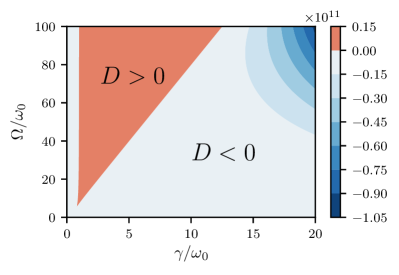
Figure 1: The discriminant of the cubic equation (26) as function of the parameters $\Omega$ and $\gamma$. Blue colours indicate negative values and red colours positive values of the discriminant.

In the blue region the discriminant is negative and hence there exist two complex solutions, while in the red region the discriminant is positive which indicates the existence of only real solutions. The factors $d_{i}$ are given by

$$d_{i}=\prod_{j\neq i}\frac{z_{i}+\Omega}{z_{j}-z_{i}}.$$ (27)

We assume a factorizing initial condition $\rho(0)=\rho_{S}\otimes\rho_{B}$, where $\rho_{S}$ is an arbitrary single mode Gaussian state and $\rho_{B}=\exp\big{(}-H_{B}/(k_{B}T)\big{)}/Z_{B}$ is a thermal equilibrium state of the bath. From this initial conditions we obtain the time evolution of the mean values

$$\langle x(t)\rangle =G_{1}(t)\langle x(0)\rangle+\frac{1}{m}G_{2}(t)\langle p(0)\rangle,$$ (28)

$$\langle p(t)\rangle =m\dot{G}_{1}(t)\langle x(0)\rangle+\dot{G}_{2}(t)\langle p(0)\rangle,$$ (29)

and the elements of the covariance matrix

$$\sigma_{xx}(t) =G_{1}^{2}(t)\sigma_{xx}(0)+\frac{1}{m^{2}}G_{2}^{2}(t)\sigma_{pp}(0)$$ (30)

$$\qquad+\frac{1}{m}G_{1}(t)G_{2}(t)\sigma_{xp}(0)+\langle I^{2}_{x}(t)\rangle,$$

$$\sigma_{pp}(t) =m^{2}\dot{G}_{1}^{2}(t)\sigma_{xx}(0)+\dot{G}_{2}^{2}(t)\sigma_{pp}(0)$$ (31)

$$\qquad+m\dot{G}_{1}(t)\dot{G}_{2}(t)\sigma_{xp}(0)+\langle I^{2}_{p}(t)\rangle,$$

$$\sigma_{px}(t) =m\dot{G}_{1}(t)G_{1}(t)\sigma_{xx}(0)+\frac{1}{m}\dot{G}_{2}(t)G_{2}(t)\sigma_{pp}(0)$$

$$\qquad+\big{(}\dot{G}_{1}(t)G_{2}(t)+\dot{G}_{2}(t)G_{1}(t)\big{)}\sigma_{xp}(0)$$

$$\qquad+\langle I^{2}_{px}(t)\rangle.$$ (32)

The crucial part in explicitly evaluating the covariance matrix for each time step is to calculate the noise contributions, which are of the form

$$\langle I_{xx}(t)\rangle =\frac{1}{2m^{2}}\int\limits^{t}_{0}ds\int\limits^{t}_{0}ds^{\prime}G_{2}(t-s)G_{2}(t-s^{\prime})\langle\{B(s),B(s^{\prime})\}\rangle,$$ (33)

$$\langle I_{pp}(t)\rangle =\frac{1}{2}\int\limits^{t}_{0}ds\int\limits^{t}_{0}ds^{\prime}\dot{G}_{2}(t-s)\dot{G}_{2}(t-s^{\prime})\langle\{B(s),B(s^{\prime})\}\rangle,$$ (34)

$$\langle I_{px}(t)\rangle =\frac{1}{2m}\int\limits^{t}_{0}ds\int\limits^{t}_{0}ds^{\prime}\dot{G}_{2}(t-s)G_{2}(t-s^{\prime})\langle\{B(s),B(s^{\prime})\}\rangle.$$ (35)

For factorizing initial conditions the correlation function $\langle\{B(t),B(t^{\prime})\}\rangle$ of the stochastic force equals the so called noise kernel $D_{1}(t-t^{\prime})$, which has the following connection to the spectral density

$$D_{1}(t-t^{\prime})=2\int\limits_{0}^{\infty}d\omega J(\omega)\coth\left(\frac{\omega}{2k_{B}T}\right)\cos\left[\omega(t-t^{\prime})\right].$$ (36)

For the Lorentz Drude spectral density it can be explicitly calculated to be

$$D_{1}(t-t^{\prime})=4m\gamma k_{B}T\Omega^{2}\sum_{n=-\infty}^{\infty}\frac{\Omega e^{-\Omega|t-t^{\prime}|}-|\nu_{n}|e^{-\nu_{n}|t-t^{\prime}|}}{\Omega^{2}-\nu_{n}^{2}},$$ (37)

where $\nu_{n}=2\pi nk_{B}T$ are the so-called Matsubara frequencies. The noise contributions can then be brought in the form

$$\langle I_{\alpha}(t)\rangle=\frac{2\gamma k_{B}T\Omega^{2}}{m}\sum_{n=-\infty}^{\infty}\frac{1}{\Omega^{2}-\nu_{n}^{2}}\mathcal{I}_{\alpha}(t,n),$$ (38)

where the index $\alpha$ stands for $xx$, $pp$ or $px$. We show in Appendix A how to explicitly calculate the factors $\mathcal{I}_{\alpha}(t,n)$. With this it is possible to determine the time evolution of the elements of the covariance matrix by numrically calculating the infinite series which appears in the noise contributions. This series turns out to converge rapidly for medium and high temperatures. Also for low temperatures evaluating the series numerically is preferable to a numerical integration of Eqs. (33)-(34).

It is also possible to derive the time evolution of the first two moments for the Caldeira-Leggett master equation

$$\frac{d}{dt}\rho_{S}(t)=-i\left[H_{S},\rho_{S}(t)\right]-i\gamma\left[x,\left\{p,\rho_{S}(t)\right\}\right]$$

$$-2m\gamma k_{B}T\left[x,\left[x,\rho_{S}(t)\right]\right]$$ (39)

which can be derived within the Born-Markov approximation under the conditions $\gamma,\omega_{0}\ll\text{Min}\{\Omega,2\pi k_{B}T\}$. From this master equation one can derive a system of coupled differential equations for the first two moments. It turns out that the solution of this coupled differential equations approximates the exact solution of the model under the under the conditions $\gamma,\omega_{0}\ll\Omega\ll 2\pi k_{B}T$. The mean values have the same structure as in Eqs. (28) and (29) with the Green’s functions

$$G_{1}(t) =\Big{[}\frac{\gamma}{\nu}\sin(\nu t)+\cos(\nu t)\Big{]}e^{-\gamma t},$$ (40)

$$G_{2}(t) =\frac{1}{\nu}\sin(\nu t)e^{-\gamma t},$$ (41)

where $\nu=\sqrt{\omega_{0}^{2}-\gamma^{2}}$. The elements of the covariance matrix have the same structure as in Eqs. (30)-(II.2) with the Green’s functions (40) and (41), and the noise contributions

$$\langle I_{xx}(t)\rangle \approx\frac{k_{B}T}{m\omega_{0}^{2}}\Bigg{[}1-e^{-2\gamma t}\Big{(}1+\frac{\gamma}{\nu}\sin(2\nu t)+2\frac{\gamma^{2}}{\nu^{2}}\sin^{2}(\nu t)\Big{)}\Bigg{]},$$ (42)

$$\langle I_{pp}(t)\rangle \approx mk_{B}T\Bigg{[}1-e^{-2\gamma t}\Big{(}\frac{\omega_{0}^{2}}{\nu^{2}}-\frac{\gamma^{2}}{\nu^{2}}\cos(2\nu t)-\frac{\gamma}{\nu}\sin(2\nu t)\Big{)}\Bigg{]},$$ (43)

$$\langle I_{px}(t)\rangle \approx 2\gamma k_{B}TG_{2}^{2}(t).$$ (44)

III Simulation results and discussion

III.1 Time evolution of the Bures distance

With help of the methods developed in the previous section we are now in the position to calculate the time evolution of the first two moments of the position and momentum operators of the open system. As initial states we consider here two pure coherent states,

$$\rho_{1}(0)=|\alpha_{1}\rangle\langle\alpha_{1}|,\qquad\rho_{2}(0)=|\alpha_{2}\rangle\langle\alpha_{2}|,$$ (45)

where

$$\alpha_{1}=\sqrt{\frac{m\omega_{0}}{2}}\langle x_{1}\rangle,\qquad\alpha_{2}=\sqrt{\frac{m\omega_{0}}{2}}\langle x_{2}\rangle.$$ (46)

To explicitly evaluate the noise contributions appearing in the covariance matrix elements we need to truncate the infinite series in Eq. (38) when sufficient accuracy is reached. For all results that we present in the following, we truncated the infinite series in the noise contribution after a number of terms $N_{c}$ such that the difference of the partial sums $\langle I_{\alpha}(t)\rangle_{(k)}$ satisfy

$$|\langle I_{\alpha}(t)\rangle_{(N_{c})}-\langle I_{\alpha}(t)\rangle_{(N_{c}-1)}|<10^{-3}$$ (47)

for every calculated time step. From the time evolution of the first two moments we are then able to compute the time evolution of the Bures distance with help of Eqs. (6) and (11).

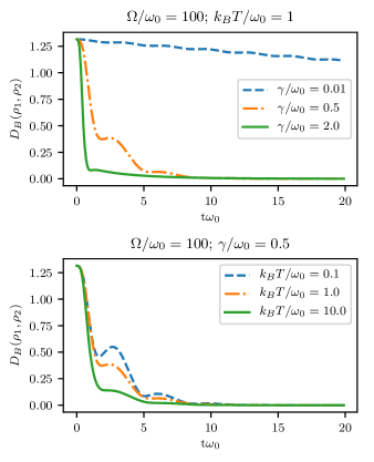
Figure 2: Time evolution of the Bures distance for different parameter combinations of the coupling strengths $\gamma$ and initial bath temperatures $T$ for a cut off $\Omega/\omega_{0}=100$. The initial states $\rho_{1}(0)$ and $\rho_{2}(0)$ are two coherent states with $\sigma_{x_{1,2}x_{1,2}}m\omega_{0}=\sigma_{p_{1,2}p_{1,2}}/(m\omega_{0})=0.5$, $\sigma_{p_{1,2}x_{1,2}}=0$ and displacements $\langle x_{1}\rangle\sqrt{2m\omega_{0}}=-1$, $\langle x_{2}\rangle\sqrt{2m\omega_{0}}=1$, as well as $\langle p_{1}\rangle=\langle p_{2}\rangle=0$.

In Figure 2 the time evolution of the Bures distance between two initial coherent states is plotted for low, medium and high coupling strengths $\gamma$ and initial bath temperatures $T$ for the cutoff frequency $\Omega/\omega_{0}=100$. The Bures distance starts in both plots nearly at its maximal value $\sqrt{2}$, indicating an almost maximal distinguishability between the initial states which are nearly orthogonal, and decreases to zero during the time evolution. Furthermore we observe clear non-monotonic behaviour of the Bures distance. We can already see from these plots, that the bumps appearing are stronger for intermediate couplings and smaller for high and low couplings. Furthermore, we see that the non-monotonicity gets stronger by lowering the initial bath temperature.

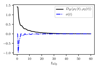
Figure 3: Black line: time evolution of the Bures distance obtained via the Caldeira-Leggett master equation. Blue line: time derivative of the Bures distance. The coupling strength is $\gamma/\omega_{0}=0.1$ and the temperature is $k_{B}T/\omega_{0}=100$. The initial states are two coherent states with variances $\sigma_{x_{1,2}x_{1,2}}m\omega_{0}=\sigma_{p_{1,2}p_{1,2}}/(m\omega_{0})=0.5$, $\sigma_{p_{1,2}x_{1,2}}=0$ and displacements $\langle x_{1}\rangle\sqrt{2m\omega_{0}}=-3$, $\langle x_{2}\rangle\sqrt{2m\omega_{0}}=3$, as well as $\langle p_{1}\rangle=\langle p_{2}\rangle=0$.

We compare this to the limiting case $\gamma,\omega_{0}\ll\Omega\ll k_{B}T$, where the dynamics of the open system can be described by the Caldeira-Leggett master equation as mentioned in the previous section. In Figure 3 we show the time evolution of the Bures distance obtained from the Caldeira-Leggett master equation and its time derivative $\sigma(t)$ for the coupling strength $\gamma/\omega_{0}=0.1$ and the initial bath temperature $k_{B}T/\omega_{0}=100$. The initial states are two coherent states with displacements $\langle x_{1}\rangle\sqrt{2m\omega_{0}}=-3$, $\langle x_{2}\rangle\sqrt{2m\omega_{0}}=3$, as well as $\langle p_{1}\rangle=\langle p_{2}\rangle=0$. We observe that $\sigma(t)$ is always negative. This implies that the Bures distance is monotonically decreasing and, hence, that our non-Markovianity measure of the dynamics is zero. Note that this fact is not obvious from the beginning since the Caldeira-Leggett master equation is not in Lindblad form.

III.2 Non-Markovianity

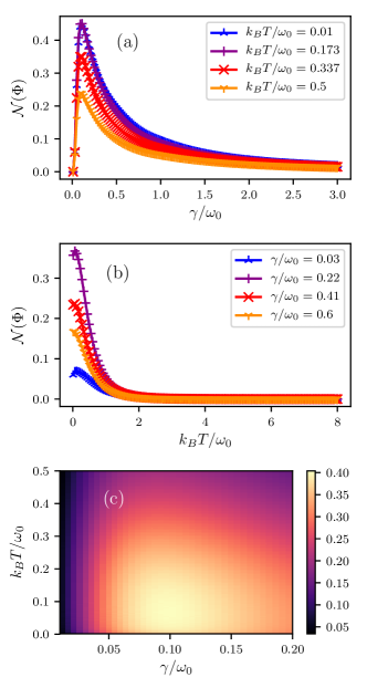
Figure 4: (a) $\mathcal{N}$ in dependence on the coupling strength $\gamma$ for different temperatures $T$. (b) $\mathcal{N}$ in dependence on the temperature $T$ for different coupling strengths $\gamma$. The maximal evaluated time is $t_{\text{max}}\omega_{0}=40$. The displacements are $\langle x_{1}\rangle\sqrt{2m\omega_{0}}=-3$, $\langle x_{2}\rangle\sqrt{2m\omega_{0}}=3$, as well as $\langle p_{1}\rangle=\langle p_{2}\rangle=0$. (c) $\mathcal{N}$ in dependence of the coupling strength $\gamma$ and the initial bath temperature $T$. The maximal evaluated time is $t_{\text{max}}\omega_{0}=25$. The displacements are $\langle x_{1}\rangle\sqrt{2m\omega_{0}}=-1$, $\langle x_{2}\rangle\sqrt{2m\omega_{0}}=1$, as well as $\langle p_{1}\rangle=\langle p_{2}\rangle=0$. In all plots the cutoff frequency is $\Omega/\omega_{0}=100$.

We continue with our main goal of this paper to characterize the non-Markovianity measure (13) in dependence on various parameters in the Caldeira-Leggett model. The numerical evaluation of the non-Markovianity measure is done as follows. Given that we calculated the time evolution of the Bures distance on a grid of $N$ points of time $t_{l}=l\Delta t$ ($l=1,...,N$) with grid size $\Delta t$, we can numerically evaluate the non-Markovianity measure by

$$\mathcal{N}(\Phi)\approx\sum_{l=0}^{N-1}\left[D_{B}(t_{l+1})-D_{B}(t_{l})\right],$$ (48)

where the sum is extended over all $l$ for which $D_{B}(t_{l+1})-D_{B}(t_{l})>0$ holds. From this it is obvious that the precision of the numerical calculation solely depends on the grid size $\Delta t$, which we chose to be $\omega_{0}\Delta t=0.01$ in the following. Furthermore we call $t_{\text{max}}=N\Delta t$ the maximal evaluated time.

We first consider the dependence of the non-Markovianity on the coupling strength $\gamma$ and on the initial bath temperature $T$. In the following plots the initial system states $\rho_{1}$ and $\rho_{2}$ are always two differently displaced coherent states with variances $\sigma_{x_{1,2}x_{1,2}}m\omega_{0}=\sigma_{p_{1,2}p_{1,2}}/(m\omega_{0})=0.5$, $\sigma_{p_{1,2}x_{1,2}}=0$.

In Fig. 4 (a) we show the non-Markovianity measure $\mathcal{N}$ in dependence on the coupling strength $\gamma$ for different temperatures of the initial bath state and a fixed frequency cutoff $\Omega/\omega_{0}=100$. We observe that $\mathcal{N}$ rapidly decreases as the coupling strength goes to zero. This can be understood from the fact that in the limiting case $\gamma/\omega_{0}\ll 1$ the dynamics is very well approximated by the quantum optical (weak coupling) master equation for the damped harmonic oscillator which is in Lindblad form and, hence, Markovian Breuer and Petruccione (2002). As can be seen from Fig. 4 (c) for sufficiently small values of $\gamma/\omega_{0}$ the non-Markovianity remains small for all temperatures, pointing to the fact that the Markov approximation is good in this regime uniformly in temperature Breuer and Petruccione (2002). At intermediate couplings we see a maximum of the non-Markovianity measure, the height of which decreases for higher temperatures. Tuning the coupling to higher values leads to a decrease of $\mathcal{N}$, which is surprising on first sight since stronger couplings should increase the ability of information exchange between system and bath.

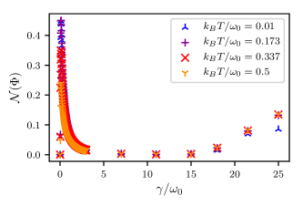
Figure 5: The non-Markovianity $\mathcal{N}$ as a function of the coupling strength $\gamma$ for different temperatures $T$. The parameters are the same as in Fig. 4 (a), but here we show a larger range of the coupling to demonstrate the increase of the non-Markovianity for very high damping.

The fact that $\mathcal{N}$ decreases to zero for increasing couplings can be understood from the following argument which holds in the strong friction Smoluchowski regime given by $\gamma/\omega_{0}\gg 1$ and $\gamma/\omega_{0}\gg\omega_{0}/k_{B}T$ Ankerhold et al. (2001); Łuczka et al. (2005). First, decoherence times are very small in the strong friction limit which leads to a very rapid decay of the off-diagonals of the density matrix in the position representation. Moreover, within the Smoluchowski regime the diagonals of the density matrix in the position representation are governed by the Smoluchowski equation which is of the form of a Fokker-Planck equation and, thus, describes a Markovian process.

What happens if one increases the coupling $\gamma$ even further such that one re-enters (for a fixed cutoff $\Omega$) the blue region of Fig. 1 in which the discriminant is negative and two complex roots of (26) exist? In view of the oscillatory nature of the solution one should expect that in this regime of ultra strong damping non-Markovian dynamics re-emerges, which is indeed confirmed by Fig. 5.

Finally, in Fig. 4(b) we observe a rapid decrease of $\mathcal{N}$ for high temperatures. At very low temperatures our simulations indicate the existence of a maximum of the non-Markovianity as a function of temperature. The height of this maximum increases below a certain value of the coupling and decreases again for higher couplings.

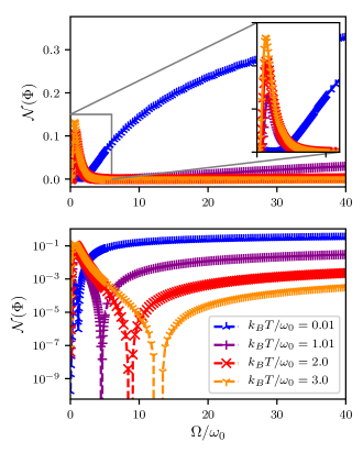
Figure 6: Top: Non-Markovianity measure $\mathcal{N}(\Phi)$ in dependence on the cutoff frequency $\Omega$ of the Lorentz-Drude spectral density for different initial bath temperatures $T$ and a fixed coupling $\gamma/\omega_{0}=0.1$. The maximal evaluated time is $t_{\text{max}}\omega_{0}=40$. The displacements are $\langle x_{1}\rangle\sqrt{2m\omega_{0}}=-3$, $\langle x_{2}\rangle\sqrt{2m\omega_{0}}=3$, as well as $\langle p_{1}\rangle=\langle p_{2}\rangle=0$. Bottom: The same plot with a logarithmic scale on the vertical axis.

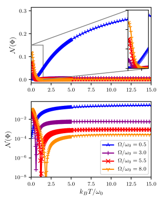
Figure 7: Top: Non-Markovianity measure $\mathcal{N}(\Phi)$ in dependence on the initial bath temperatures $T$ for different cutoff frequencies $\Omega$ of the Lorentz-Drude spectral density and a fixed coupling $\gamma/\omega_{0}=0.1$. The maximal evaluated time is $t_{\text{max}}\omega_{0}=40$. The displacements are $\langle x_{1}\rangle\sqrt{2m\omega_{0}}=-3$, $\langle x_{2}\rangle\sqrt{2m\omega_{0}}=3$, as well as $\langle p_{1}\rangle=\langle p_{2}\rangle=0$. Bottom: The same plot with a logarithmic scale on the vertical axis.

Next, we consider the non-Markovianity in dependence on the cutoff frequency $\Omega$ and the initial bath temperature $T$. Figure 6 shows the non-Markovianity as a function of the cutoff frequency $\Omega$ for different initial bath temperatures $T$. The system-bath coupling is fixed to $\gamma/\omega_{0}=0.1$. The first point one notices in the upper plot of Fig. 6 is that there exists a local maximum not far from the cutoff frequency $\Omega/\omega_{0}=1$, which increases and slightly shifts to lower cutoffs for higher temperatures. In the bottom plot we show the same graphs on a logarithmic scale in the vertical axis. This also reveals a minimum of the non-Markovianity measure, which moves to higher cutoffs and gets broader for increasing temperatures. We will come back to an explanation of this feature below.

In Fig. 7 we present the non-Markovianity measure $\mathcal{N}$ in dependence on the initial bath temperature $T$ for different cutoff frequencies $\Omega$ and a fixed coupling $\gamma/\omega_{0}=0.1$. Also here we can see from the upper plot a maximum at very low temperatures. After this maximum $\mathcal{N}$ drops rapidly for increasing temperature. The bottom plot, where the vertical axis has a logarithmic scale, reveals again a minimum of $\mathcal{N}$ which moves to higher temperatures for increasing cutoffs. The dependence of this minimum on the cutoff and the temperature can be seen in the top plot of Fig. 8. In the bottom plot of Fig. 8 we show for a comparison the results of a similar study on the non-Markovianity measure in the spin-boson model Clos and Breuer (2012). The authors of this study investigated the originally proposed non-Markovianity measure involving the trace distance and carried out the maximization procedure by a random sampling of the initial states over the whole Bloch sphere. Furthermore, they utilized the second-order Born approximation of the master equation (without the Markov approximation) in order determine the dynamics of the spin. It is quite remarkable that, despite all these differences $\mathcal{N}(\Omega,T)$ behaves almost the same in both models. The main reasons for these striking similarities are on the one hand the close relationship between the trace distance and the Bures distance and, on the other hand, the fact that both models describe an open system with a single transition frequency $\omega_{0}$, a linear system-bath interaction and the same spectral density.

In order to explain the cutoff and temperature dependent minimum of the non-Markovianity discussed above we employ an argument developed in Ref. Clos and Breuer (2012). This argument is based on the effective spectral density

$$J_{\text{eff}}(\omega,\Omega,T)=J(\omega,\Omega)\coth\left(\frac{\omega}{2k_{B}T}\right)$$ (49)

which determines the frequency spectrum of the noise kernel defined in Eq. (36). If the effective spectral density is maximal at $\omega=\omega_{0}$ the oscillator ‘feels’ a spectral density which is approximately constant in the vicinity of its eigenfrequency $\omega_{0}$ and, therefore, approximately corresponds to the spectrum of white noise favoring Markovian behavior. The idea is thus that

$$\left.\frac{\partial J_{\text{eff}}(\omega,\Omega,T)}{\partial\omega}\right|_{\omega=\omega_{0}}=0$$ (50)

is an appropriate condition for predominantly Markovian dynamics. It is easy to verify that this resonance condition yields a curve in the $(\Omega,T)$ plane which is given by

$$\Omega=\omega_{0}\sqrt{\frac{k_{B}T\sinh\left(\frac{\omega_{0}}{k_{B}T}\right)+\omega_{0}}{k_{B}T\sinh\left(\frac{\omega_{0}}{k_{B}T}\right)-\omega_{0}}}$$ (51)

and shown as white curves in Fig. 8. As can be seen from the figure the resonance condition very well reproduces the location of the minima of the non-Markovinaity measure.

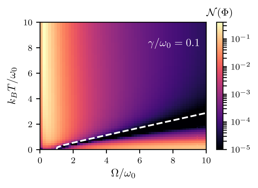
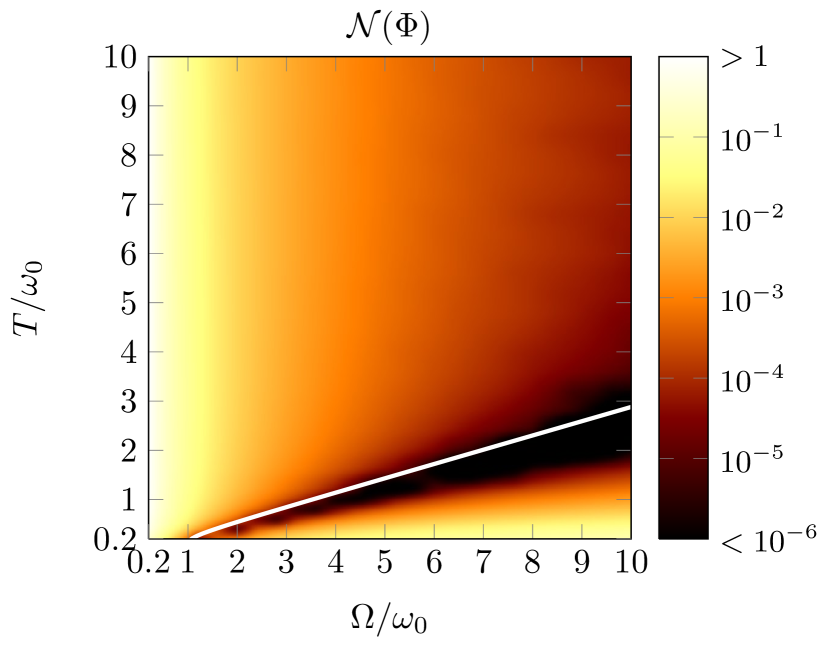
Figure 8: Top: Non-Markovianity measure for the Caldeira-Leggett model in dependence on $\gamma$ and $\Omega$. The initial states were two coherent states with displacements $\langle x_{1}\rangle\sqrt{2m\omega_{0}}=-3$, $\langle x_{2}\rangle\sqrt{2m\omega_{0}}=3$, and $\langle p_{1}\rangle=\langle p_{2}\rangle=0$. The maximal evaluated time is $t_{\text{max}}\omega_{0}=25$. The coupling is fixed to $\gamma/\omega_{0}=0.1$ Bottom: Non-Markovianity measure defined with help of the trace distance in dependence on temperature $T$ and cutoff frequency $\Omega$ for the Spin-Boson model by the second-order Born approximation Clos and Breuer (2012). The coupling was fixed to $\gamma/\omega_{0}=0.1$. The initial states of the spin correspond to antipodal points of the Bloch sphere. In both plots the white curve represents the resonance condition of Eq. (51).

III.3 Influence of external driving on non-Markovianity

Finally, we investigate the impact of an external force on the non-Markovianity measure, driving the open system and/or the bath modes. Remarkably, it turns out that driving does not influence the non-Markovianity in our case. This is in contrast to other studies, which have investigated the influence of driving on a similar measure of non-Markovianity on an open two-level systems, for example in Ref. Poggi et al. (2017). In Sampaio et al. (2017) it was shown that the system driving can even increase non-Markovian effects.

A general driving of the system or bath modes results in an additional term in the Hamiltonian (II.2) of the form

$$H_{\text{ext}}(t)=-\left(d_{0}x+\sum_{n}d_{n}x_{n}\right)F(t),$$ (52)

where the $d_{\alpha}$ represent the driving strengths of the system and the bath modes and $F(t)$ is the external force. It is straightforward to repeat the derivation of the Heisenberg equation (18) taking into account the terms stemming from the external Hamiltonian contribution (52). The result is

$$\ddot{x}(t)+\omega_{0}^{2}x(t)+\frac{d}{dt}\int\limits_{0}^{t}dt^{\prime}\gamma(t-t^{\prime})x(t^{\prime})=\frac{1}{m}(B(t)+F_{\text{eff}}(t)),$$ (53)

where

$$F_{\text{eff}}(t)=d_{0}F(t)+\int\limits_{0}^{t}dt^{\prime}\Lambda(t-t^{\prime})F(t^{\prime})$$ (54)

with $\Lambda(t)=\sum_{n}\frac{d_{n}\kappa_{n}}{m_{n}\omega_{n}}\sin\left(\omega_{n}t\right)$ is the effective driving force consisting of the direct external driving of the system and the indirect driving mediated by the bath Grabert and Thorwart (2018). We again solve this equation via a Laplace transformation. This results in an additional term

$$x_{D}(t)=\frac{1}{m}\int\limits_{0}^{t}dt^{\prime}G_{2}(t-t^{\prime})F_{\text{eff}}(t^{\prime})$$ (55)

to the previously obtained solution of Eq. (21), which we now call $x_{H}(t)$ such that

$$x(t)=x_{H}(t)+x_{D}(t).$$ (56)

Since the driving term $x_{D}(t)$ is a c-number function it follows that

$$\big{\langle}x_{D}^{2}(t)\big{\rangle} =\big{\langle}x_{D}(t)\big{\rangle}^{2},$$ (57)

$$\big{\langle}x_{H}(t)x_{D}(t)\big{\rangle} =\big{\langle}x_{H}(t)\big{\rangle}\big{\langle}x_{D}(t)\big{\rangle},$$ (58)

which means that the driving term has no influence on the position variance. Analogously, one can see that the driving term has also no influence on the other elements of the covariance matrix. Still, the mean values of the position and momentum are affected and are given by

$$\big{\langle}x(t)\big{\rangle} =\big{\langle}x_{H}(t)\big{\rangle}+\int\limits_{0}^{t}dt^{\prime}G_{2}(t-t^{\prime})F_{\text{eff}}(t^{\prime}),$$ (59)

$$\big{\langle}p(t)\big{\rangle} =\big{\langle}p_{H}(t)\big{\rangle}+\int\limits_{0}^{t}dt^{\prime}\dot{G}_{2}(t-t^{\prime})F_{\text{eff}}(t^{\prime}).$$ (60)

However, in the expression (6) for the quantum fidelity of Gaussian states only the difference between the mean values $\mathbf{d}_{2}-\mathbf{d}_{1}$ enters, such that the driving contributions cancel each other since they are independent of the initial conditions. Hence, the fidelity is not influenced by the driving of the system and/or bath modes and thus also the non-Markovianity measure remains unaffected. The above derivation shows that the main reasons for this fact are the Gaussian nature of the initial states and the linearity of the model.

IV Conclusions

In this article we investigated the emergence of memory effects in the Caldeira-Leggett model for different parameter regimes of the coupling strength, the frequency cutoff of the spectral density and the bath temperature. We quantified non-Markovianity with help of a measure especially suitable for continuous variable systems, which is based on the Bures metric as distance measure for quantum states. We used Gaussian initial states for the open system which allowed us to exactly determine the time evolution for arbitrary parameter combinations without any approximation.

Our main results may be summarized as follows.

• We found that the non-Markovianity measure exhibits a non-monotonic behaviour as a function of the coupling strength and the bath temperature. In particular, it shows a maximum at intermediate coupling strengths and decreases for higher values of the latter (see Sec. III.2).

• For small coupling strength the non-Markovianity measure as a function of frequency cutoff and temperature shows remarkable similarities to the spin-boson model for which an analogous study is discussed in Ref. Clos and Breuer (2012). In both models one finds a pronounced Markovian area (minimum of the non-Markovianity measure) inside a non-Markovian regime which can be understood as a resonance effect resulting from the maximum of an effective, temperature-dependent spectral density (see, in particular, Eq. (50)).

• The decrease of the non-Markovianity with increasing coupling strength in the regime of strong dissipation can be explained as resulting from the dynamical behavior in the Smoluchowski regime Ankerhold et al. (2001); Łuczka et al. (2005). In addition, we observe an anew increase of the non-Markovianity for ultra strong coupling (see Sec. III.2).

• We showed that non-Markovianity cannot be generated within the approximation provided by the Caldeira-Leggett master equation for Gaussian initial states (see Sec. III.1).

• Finally, we demonstrated that a driving of the system and/or the bath modes by an arbitrary external force has no influence on the non-Markovianity of the open system dynamics which is due to the linearity of the model and the use of Gaussian initial states (see Sec. III.3).

In summary, we observed a rich behavior of the non-Markovianity of quantum Brownian motion, even though our model is linear and thus integrable. Several of the features described obviously depend on the linearity and on the Gaussian character of the initial states. We expect that further interesting phenomena emerge if one considers a nonlinear open system or non-Gaussian initial states. Another interesting problem is to study further the relations between different physical models with regard to their degree of non-Markovianity. Our findings on the similarity between quantum Brownian motion and the spin-boson model point to a kind of universality of non-Markovian behavior which should be scrutinized in more detail.

Appendix A Calculation of the Noise contributions

We illustrate the procedure of determining the noise integrals (33)-(35) by means of $\langle I_{xx}(t)\rangle$ in the following. We have

$$\langle I_{xx}(t)\rangle=\frac{2\gamma k_{B}T\Omega^{2}}{m}\sum_{n=-\infty}^{\infty}\frac{1}{\Omega^{2}-\nu_{n}^{2}}\mathcal{I}(t,n),$$ (61)

where

$$\mathcal{I}(t,n) =\int^{t}_{0}ds\int^{t}_{0}ds^{\prime}G_{2}(t-s)G_{2}(t-s^{\prime})\left(\Omega e^{-\Omega|s-s^{\prime}|}-|\nu_{n}|e^{-|\nu_{n}||s-s^{\prime}|}\right)$$ (62)

$$=\sum_{i,j=1}^{3}d_{i}d_{j}e^{(z_{i}+z_{j})t}\int^{t}_{0}ds\int^{t}_{0}ds^{\prime}e^{-(z_{i}s+z_{j}s^{\prime})}\left(\Omega e^{-\Omega|s-s^{\prime}|}-|\nu_{n}|e^{-|\nu_{n}||s-s^{\prime}|}\right).$$ (63)

We change to the new integration variables $\tilde{s}=s-s^{\prime}$ and $\tau=s^{\prime}$. This leads to

$$\mathcal{I}(t,n)=\sum_{i,j=1}^{3}d_{i}d_{j}e^{(z_{i}+z_{j})t}\int^{t}_{0}d\tau\int^{t-\tau}_{-\tau}d\tilde{s}e^{-(z_{i}(\tilde{s}+\tau)+z_{j}\tau)}\left(\Omega e^{-\Omega|\tilde{s}|}-|\nu_{n}|e^{-|\nu_{n}||\tilde{s}|}\right).$$ (64)

The time integrals can be evaluated straightforwardly to obtain the expression

$$\begin{split}\mathcal{I}(t,n)=\sum_{i,j=1}^{3}d_{i}d_{j}&\Bigg{\{}\frac{|\nu_{n}|}{|\nu_{n}|-z_{i}}\bigg{(}\frac{1-e^{(z_{i}+z_{j})t}}{z_{i}+z_{j}}-\frac{e^{(-|\nu_{n}|+z_{i})t}-e^{(z_{i}+z_{j})t}}{|\nu_{n}|+z_{j}}\bigg{)}\\ &-\frac{\Omega}{\Omega-z_{i}}\bigg{(}\frac{1-e^{(z_{i}+z_{j})t}}{z_{i}+z_{j}}-\frac{e^{(-\Omega+z_{i})t}-e^{(z_{i}+z_{j})t}}{\Omega+z_{j}}\bigg{)}\\ &+\frac{|\nu_{n}|}{|\nu_{n}|+z_{i}}\bigg{(}\frac{1-e^{(z_{j}-|\nu_{n}|)t}}{|\nu_{n}|-z_{j}}+\frac{1-e^{(z_{i}+z_{j})t}}{z_{i}+z_{j}}\bigg{)}-\frac{\Omega}{\Omega+z_{i}}\bigg{(}\frac{1-e^{(z_{j}-\Omega)t}}{\Omega-z_{j}}+\frac{1-e^{(z_{i}+z_{j})t}}{z_{i}+z_{j}}\bigg{)}\Bigg{\}}.\end{split}$$ (65)

References

- Breuer and Petruccione (2002) H.-P. Breuer and F. Petruccione, The Theory of Open Quantum Systems (Oxford University Press, Oxford, 2002).
- Rivas et al. (2014) A. Rivas, S. F. Huelga, and M. B. Plenio, Rep. Prog. Phys. 77, 094001 (2014).
- Breuer et al. (2016) H.-P. Breuer, E.-M. Laine, J. Piilo, and B. Vacchini, Rev. Mod. Phys. 88, 021002 (2016).
- de Vega and Alonso (2017) I. de Vega and D. Alonso, Rev. Mod. Phys. 89, 015001 (2017).
- Apollaro et al. (2011) T. J. G. Apollaro, C. Di Franco, F. Plastina, and M. Paternostro, Phys. Rev. A 83, 032103 (2011).
- Haikka et al. (2011) P. Haikka, S. McEndoo, G. De Chiara, G. M. Palma, and S. Maniscalco, Phys. Rev. A 84, 031602 (2011).
- Haikka et al. (2012) P. Haikka, J. Goold, S. McEndoo, F. Plastina, and S. Maniscalco, Phys. Rev. A 85, 060101 (2012).
- Gessner et al. (2014a) M. Gessner, M. Ramm, H. Häffner, A. Buchleitner, and H.-P. Breuer, EPL 107, 40005 (2014a).
- Gröblacher et al. (2015) S. Gröblacher, A. Trubarov, N. Prigge, G. D. Cole, M. Aspelmeyer, and J. Eisert, Nature Communications 6, 7606 (2015).
- Znidaric et al. (2011) M. Znidaric, C. Pineda, and I. García-Mata, Phys. Rev. Lett. 107, 080404 (2011).
- García-Mata et al. (2012) I. García-Mata, C. Pineda, and D. Wisniacki, Phys. Rev. A 86, 022114 (2012).
- Rebentrost and Aspuru-Guzik (2011) P. Rebentrost and A. Aspuru-Guzik, J. Chem. Phys. 134, 101103 (2011).
- Green et al. (2019) D. Green, B. S. Humphries, A. G. Dijkstra, and G. A. Jones, The Journal of Chemical Physics 151, 174112 (2019), https://doi.org/10.1063/1.5119300 .
- Vasile et al. (2011a) R. Vasile, S. Olivares, M. Paris, and S. Maniscalco, Phys. Rev. A. 83, 042321 (2011a).
- Chin et al. (2012) A. W. Chin, S. F. Huelga, and M. B. Plenio, Phys. Rev. Lett. 109, 233601 (2012).
- Liu et al. (2011) B.-H. Liu, L. Li, Y.-F. Huang, C.-F. Li, G.-C. Guo, E.-M. Laine, H.-P. Breuer, and J. Piilo, Nature Physics 7, 931 (2011).
- Li et al. (2011) C.-F. Li, J.-S. Tang, Y.-L. Li, and G.-C. Guo, Phys. Rev. A 83, 064102 (2011).
- Smirne et al. (2011) A. Smirne, D. Brivio, S. Cialdi, B. Vacchini, and M. G. A. Paris, Phys. Rev. A 84, 032112 (2011).
- Gessner et al. (2014b) M. Gessner, M. Ramm, T. Pruttivarasin, A. Buchleitner, H.-P. Breuer, and H. Häffner, Nature Physics 10, 105 (2014b).
- Cialdi et al. (2014) S. Cialdi, A. Smirne, M. G. A. Paris, S. Olivares, and B. Vacchini, Phys. Rev. A 90, 050301 (2014).
- Tang et al. (2015) J.-S. Tang, Y.-T. Wang, G. Chen, Y. Zou, C.-F. Li, G.-C. Guo, Y. Yu, M.-F. Li, G.-W. Zha, H.-Q. Ni, Z.-C. Niu, M. Gessner, and H.-P. Breuer, Optica 2, 1014 (2015).
- Breuer et al. (2009) H.-P. Breuer, E.-M. Laine, and J. Piilo, Phys. Rev. Lett. 103, 210401 (2009).
- Helstrom (1976) C. W. Helstrom, Quantum Detection and Estimation Theory (Academic Press, New York, 1976).
- Hayashi (2006) M. Hayashi, Quantum Information (Springer, Berlin, 2006).
- Caldeira and Leggett (1983) A. Caldeira and A. Leggett, Annals of Physics 149, 374 (1983).
- Grabert et al. (1988) H. Grabert, P. Schramm, and G.-L. Ingold, Physics Reports 168, 115 (1988).
- Vasile et al. (2011b) R. Vasile, S. Maniscalco, M. G. A. Paris, H.-P. Breuer, and J. Piilo, Phys. Rev. A 84, 052118 (2011b).
- Laine et al. (2010) E.-M. Laine, J. Piilo, and H.-P. Breuer, Phys. Rev. A 81, 062115 (2010).
- Chruściński et al. (2011) D. Chruściński, A. Kossakowski, and A. Rivas, Phys. Rev. A 83, 052128 (2011).
- Wißmann et al. (2015) S. Wißmann, B. Vacchini, and H.-P. Breuer, Phys. Rev. A 92, 042108 (2015).
- Bengtsson and Zyczkowski (2006) I. Bengtsson and K. Zyczkowski, Geometry of Quantum States: An Introduction: An Introduction to Quantum Entanglement (Cambridge University Press, UK, 2006).
- Ankerhold et al. (2001) J. Ankerhold, P. Pechukas, and H. Grabert, Phys. Rev. Lett. 87, 086802 (2001).
- Łuczka et al. (2005) J. Łuczka, R. Rudnicki, and P. Hänggi, Physica A: Statistical Mechanics and its Applications 351, 60 (2005).
- Clos and Breuer (2012) G. Clos and H.-P. Breuer, Phys. Rev. A 86, 012115 (2012).
- Poggi et al. (2017) P. M. Poggi, F. C. Lombardo, and D. A. Wisniacki, EPL (Europhysics Letters) 118, 20005 (2017).
- Sampaio et al. (2017) R. Sampaio, S. Suomela, R. Schmidt, and T. Ala-Nissila, Phys. Rev. A 95, 022120 (2017).
- Grabert and Thorwart (2018) H. Grabert and M. Thorwart, Phys. Rev. E 98, 012122 (2018).