Effective epidemic model for COVID-19 using accumulated deaths

Abstract

The severe acute respiratory syndrome COVID-19 has been in the center of the ongoing global health crisis in 2020. The high prevalence of mild cases facilitates sub-notification outside hospital environments and the number of those who are or have been infected remains largely unknown, leading to poor estimates of the crude mortality rate of the disease. Here we use a simple model to describe the number of accumulated deaths caused by COVID-19. The close connection between the proposed model and an approximate solution of the SIR model provides a system of equations whose solutions are robust estimates of epidemiological parameters. We find that the crude mortality varies between $10^{-4}$ and $10^{-3}$ depending on the severity of the outbreak which is lower than previous estimates obtained from laboratory confirmed patients. We also estimate quantities of practical interest such as the basic reproduction number and the expected number of deaths in the asymptotic limit with and without social distancing measures and lockdowns, which allow us to measure the efficiency of these interventions.

1 Introduction

Outbreaks of infectious diseases have been a common occurrence throughout history, often linked or followed by disruptions in societies and human activities [1]. There are several ways to measure the impact of outbreaks but death tolls are the most relevant ones whenever the disease can threaten lives. For instance, 32 million persons have died between 1981 and 2019 in the ongoing HIV epidemics, 700 000 in 2018 alone [2]. Aside from this large scale epidemic, the world has experienced several other recent outbreaks with varying degrees of severity and scale: Zika fever, whose symptoms are mild but can produce long-lasting effects in newborns (microcephaly) [3, 4]; Ebola virus disease, with a high mortality rate estimated between 20 and 75% [5, 6]; Swine flu/H1N1, which became a pandemic in 2009-2010 although with a lower mortality rate than regular flu [7]. In 2019-2020, the severe acute respiratory syndrome COVID-19 has emerged as the most recent pandemic, caused by the virus named SARS-CoV-2 [8, 9]. Due to its novelty and lack of previous exposition, humans have no immunity against this threat, leading to increased number of infections. At the time of this writing, the specifics of the pathogen transmission are still being investigated, as well as the complete infection process once the virus enters the host. However, it has been shown that the main human-to-human transmission mode occurs by the spreading of contaminated droplets, similar to other flu-like diseases [8]. In sharp contrast with H1N1, however, the mortality rate of COVID-19 is estimated in the range 1-4%, with higher ill-outcomes among persons of old age [10, 11]. This situation creates a unique scenario where healthcare facilities and workers can be overwhelmed in a short period of time, ultimately leading to untreated patients of COVID-19 as well as other diseases [12].

To make matters even worse, asymptomatic patients can spread the pathogen for an extended period of time, showing none or mild symptoms during the course of the infection. As a result, laboratory tests to detect the viral load are necessary to identify the correct number of cases outside hospital environments. Similar to the H1N1 pandemic, the required number of tests far exceeds the current amount available in most countries. Without timely tracking of new cases, contact tracing becomes a challenging task, hindering estimates of new cases per infection summarized by the basic reproduction number, $\mathcal{R}_{0}$. The significance of this parameter lies in the fact that it provides a way to glimpse the values of the transmission rates. Those can then be used in compartmental models – mathematical models that describe the evolution of epidemics assuming nearly homogeneous populations [13, 14]. Earlier estimates for $\mathcal{R}_{0}$ using epidemiological data from Wuhan, China, set $\mathcal{R}_{0}$ between $1.5$ to $5.7$ without additional measures to restrict the spreading [15, 16, 17]. With measures in place – such as lockdown, self-isolation, and social distancing – $\mathcal{R}_{0}$ was estimated to be around $1.05$ [15]. More importantly, the insufficient number of tests, in addition to the long waiting time for lab results, affects the quality of epidemic models.

In the absence of mass testings, the death toll can be used as an alternative metric to probe the extension of the epidemic. The medical staff can assess the cause of death from clinical reports, which may contain test results or not, using the best of their knowledge. Additional tests may also be appended to reports to further specify the cause of death.

Both numbers of cases and deaths are publicly available as part of a global effort to tackle the pandemic. Here, we study the evolution of COVID-19 deaths in order to reduce the issues caused by the limited number of laboratory confirmed tests. We show that the accumulated deaths can be effectively described by simple functions, namely, sigmoids whose parameters are explained in terms of the SIR epidemic model. The SIR model is a compartmental model with the following health states: susceptible, infective, and removed [18]. The removed state represents those who have passed away or have developed immunity, either by recovering from the disease or any other method such as vaccination. The SIR model was chosen in detriment of epidemic models with additional health states or reinfections because it is the simplest model that addresses immunity. Among our results, we show that crude mortality rates can be computed from the parameters of sigmoids and that the rates can change up to one order of magnitude, depending on the severity of the outbreak in a given region. The paper is organized as follows. Sec. 2 contains the description of the data and variables used along the text. Sec. 3 explains how the SIR model is reduced from a system of differential equations to a single non-linear differential equation, with emphasis on the expansion around equilibrium. Data is modeled in Sec. 4 via sigmoidal functions, whose parameters are explained in terms of the epidemiological parameters of the SIR model. Time windows are addressed in Sec. 5, with special emphasis on $\mathcal{R}_{0}$, crude mortality rate, and quantitative effects of the confinement. Final comments and conclusions are listed in Sec 6.

2 Data

The European Center for Disease Prevention and Control (ECDC) provides COVID-19 data updated in a daily schedule [19]. The daily reports portray the distribution of new confirmed cases and new deaths presented as time series. The dataset also displays the population size $N$ according to 2018 World Bank census for each geographical region (see Table 1).

Table 1: Example of ECDC time series for daily number of new cases and new deaths in France [19].

date	day	month	year	cases	deaths	country	geoId	country code	$N$
08/04/2020	8	4	2020	3777	1417	France	FR	FRA	66987244
07/04/2020	7	4	2020	3912	833	France	FR	FRA	66987244
06/04/2020	6	4	2020	1873	518	France	FR	FRA	66987244
05/04/2020	5	4	2020	4267	1053	France	FR	FRA	66987244
04/04/2020	4	4	2020	5233	2004	France	FR	FRA	66987244

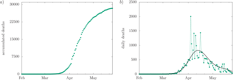
Figure 1: Evolution of COVID-19 deaths in France. a) Accumulated COVID-19 deaths (circles). Countrywide measures to increase social distance and enforce confinement were introduced on March 16, and progressively removed starting from May 11 in a per region criteria. b) Asymmetry of the daily deaths (dotted line) in France induced by measures to control and reduce the spreading of the virus among the population. (Solid line) Bézier curve for 7 days moving average for daily deaths.

To better grasp the nature of the data, consider the number of accumulated deaths in France, as shown in Fig. 1. Similar to other European countries, France was heavily affected by the pandemic nearing the mark of 30 000 deaths, with a sharp increase in deaths of infected patients around April-May. These deaths are linked to infections which took place between 3 to 6 weeks prior. On March 16, the French government implemented measures to mitigate the propagation of the disease. The measures included confinement of non-essential workers and temporary closures of schools and universities, as well as commercial stores and services. The effects of said measures did not show up immediately on the data (see Fig. 1b) but instead they appeared after some time had passed, around 4 weeks, reducing the number of daily fatalities.

Before diving into modeling, we seek for general features that can be used to model outbreaks. These features concern the spreading regime of the disease among the population, excluding spatial effects and temporal delays. As noted above, the death toll experienced a rapid growth between March and April (see Fig. 1). This regime is the hallmark of epidemics and denotes the exponential phase. In general, the growth rate in compartmental epidemic models is summarized by $\mathcal{R}_{0}$ that is the ratio of the transmission rate $\alpha$ to the removal rate $\lambda$. As the name implies, the transmission rate dictates the average number of persons a given infective individual typically infects during a fixed time interval. The inverse of the removal rate is the characteristic time in which a person remains contagious.

The inflection point is another important feature. However, unlike small scale outbreaks, where the disease spreads uninterruptedly among elements of a given population, the introduction of large scale control measures forcibly modifies the transmission rate. This sudden perturbation reduces the value of the transmission rate in a short time interval, creating an artificial inflection point.

After the exponential phase, the system relaxes toward an equilibrium state with no infective people, with a characteristic time scale, namely, the relaxation time $\tau$. We shall investigate the relationship between $\tau$ with epidemiological parameters in the next section. Considering these three aspects, and using Fig. 1 as reference, it becomes clear that the number of accumulated deaths is a monotonic function, with an early exponential growth only to be replaced by a smooth relaxation towards equilibrium. Therefore, sigmoids appears as ideal candidates to model the data.

3 SIR model

For the sake of simplicity, let us assume the spreading dynamics can be approximated by the standard SIR model in a homogeneous population of size $N$. The model comprises a population whose subjects can be classified in three distinct health states, namely, susceptible, infective, and removed. The removed state includes individuals that have either died or recovered from the disease. The latter are assumed to not be infective anymore, nor susceptible to become sick again because of some kind of immunity. The fraction of individuals in each compartment is, respectively, $S(t)$, $I(t)$, and $R(t)$, at time instant $t$. The dynamic goes as follows. Infective subjects in the population transmit the pathogen to susceptible ones, under adequate conditions. The transmission occurs with rate $\alpha$, and we assume the homogeneous mixture of the population, that is, each person in the population is statistically equivalent to each other [14]. Once infected, the person remains infective for an average period $1/\lambda$, where $\lambda$ is the removal rate. The dynamical equations that describe the model are:

$$\frac{dS}{dt} =-\alpha S(t)I(t),$$ (1a)

$$\frac{dI}{dt} =+\alpha S(t)I(t)-\lambda I(t),$$ (1b)

$$\frac{dR}{dt} =+\lambda I(t),$$ (1c)

with the constraint $S+I+R=1$, i.e., conservation of the population size. The model certainly simplifies or neglects recent aspects of the COVID-19 pandemic such as differentiation between asymptomatic and symptomatic transmission or age-dependent rates [20, 21]. In fact, research on the biological characteristics of the ongoing pandemic are still ongoing [22], but evidence indicates re-infections should be minimal in recovered patients [23]. Therefore, we make a case for an approximate description of the problem via the SIR model over the inclusion of extra complexities and uncertainties, aiming to capture dominant aspects.

The system of differential equations (1a-1c) can be further reduced to a single first-order differential equation as follows. From (1c) and (1a), one finds $S(t)=S_{0}\textrm{e}^{-(\alpha/\lambda)\,R(t)}$. The constant $S_{0}=S(0)\textrm{e}^{(\alpha/\lambda)\,R(0)}$ depends on the initial conditions $S(0)$ and $R(0)=1-S(0)-I(0)$. Usually, we are more interested in scenarios in which $R(0)=0$ and thus $S_{0}=1-I(0)$, similar to the onset of an emerging disease. The complete expression for $S_{0}$ must be used for different initial conditions, which can become a problem whenever the ratio $\alpha/\lambda$ is unknown. Ignoring constant solutions, it can be shown [24] that the equation can be further reduced to

$$\frac{dR}{dt}=-\lambda S_{0}\textrm{e}^{-(\alpha/\lambda)R(t)}-\lambda R+\lambda,$$ (2)

whose general solution can be obtained by quadrature

$$t-t_{0}=\frac{1}{\lambda}\int_{R(0)}^{R(t)}\frac{dr}{1-r-S_{0}\textrm{e}^{-(\alpha/\lambda)r}}.$$ (3)

The stationary condition in (2) gives the value $R_{\infty}$ as a solution of the transcendental equation $R_{\infty}=1-S_{0}\textrm{e}^{-(\alpha/\lambda)R_{\infty}}$.

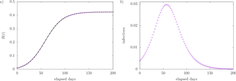
Figure 2: SIR model. a) Numerical solution of the SIR model (empty circles) with $\mathcal{R}_{0}=1.3$. A good agreement is found between the sigmoidal curve (5) whose parameters were found by least-square fitting (line) and the SIR model, being less accurate for increasing values of $\mathcal{R}_{0}$. b) The curve that represents the infective fraction of the population in the SIR model is symmetrical, with peak at the center, as long as parameters remain constant.

The solution $R(t)$ can be obtained by inverting (3), for which a general method remains unknown. To circumvent the issue, one may expand (2) around points of interest, for example, around $R=0$ or $R=R_{\infty}$. Each expansion has advantages and issues. The linear term in the expansion around $R=0$ dictates the exponential growth of $R(t)$, with an effective rate $\alpha S_{0}-\lambda$. We use the adjective effective rather loosely here because at some point the curve should change its curvature and converge to an equilibrium value. Unfortunately, the competition between the early exponential growth and relaxation towards equilibrium is often difficult to assess near the onset of the outbreak, requiring higher order contributions in the expansion.

Alternatively, we can get a better picture of the problem by expanding $R(t)$ around the equilibrium. By doing so, the expansion only requires contributions up to second order, as it already carries the information regarding $R_{\infty}$. Furthermore, the expansion near the equilibrium also ensures that $\tau$ describes the dominant relaxation time, rather than combinations of several decay modes, each one with its own timescale. Define $\delta R(t)=R_{\infty}-R(t)\geqslant 0$. The expansion of (2) near $\delta R\ll 1$, together with the transcendental equation for $R_{\infty}$, gives

$$\frac{1}{\lambda}\frac{d}{dt}\delta R=-\left[1-(1-R_{\infty})\frac{\alpha}{\lambda}\right]\delta R+\frac{1-R_{\infty}}{2}\,\left(\frac{\alpha}{\lambda}\right)^{2}\delta R^{2}+o(\delta R^{3}).$$ (4)

Keeping terms up to $o(\delta R^{2})$, one converts (4) into a Bernoulli equation with relaxation time $\tau=[\lambda-\alpha(1-R_{\infty})]^{-1}$. Solving for $\delta R$ and transforming back to $R$, we find the approximate solution (see Fig. 2)

$$R(t)=\frac{R_{\infty}-A\,\textrm{e}^{-t/\tau}}{\;\;\;\;1+B\,\textrm{e}^{-t/\tau}}\;,$$ (5)

with $A=R_{\infty}-(1+B)R(0)$, $B=c_{0}\tau/z_{0}$, $\,z_{0}=[R_{\infty}-R(0)]^{-1}-c_{0}\tau$, and $c_{0}=(\lambda/2)(1-R_{\infty})(\alpha/\lambda)^{2}$.

4 Effective model

The sigmoidal expression in (5) satisfies the requirements listed in Sec. 2 and it is an excellent candidate to model the data of accumulated deaths. However, the removed compartment corresponding to $R(t)$ holds both recovered and deceased fractions of the population, i.e., all the infected who are unable to spread the disease. We can simplify this issue by assuming the existence of a simple relation between $R(t)$ and the accumulated number of deaths divided by the population size, $g(t)$, at the time instant $t$. To keep the model as simple as possible, we neglect temporal delays and impose

$$g(t)=fR(t),$$ (6)

where the crude mortality rate $f$ is the ratio between deceased and infected. As such, it also can be used as an estimator for the likelihood to die after contracting the disease.

The equilibrium value $g_{\infty}$ varies from country to country and can be used to characterize the outbreak, more specifically, to assess the impact of the outbreak in the afflicted population. The monotonic nature of cumulative quantities together with the upper bound $g_{\infty}$ restrict the possible functional forms for $g(t)$. Sigmoids are natural candidates to describe $g(t)$ since they are bounded and monotonic. Here we consider the following expression in tandem with (5):

$$g_{\textrm{eff}}(t)\equiv\frac{g_{\infty}-a\,\textrm{e}^{-t/\tau}}{1+b\,\textrm{e}^{-t/\tau}}.$$ (7)

The timescale $\tau$ dictates the relaxation of $g(t)$ towards $g_{\infty}$, with inflection at $t_{c}=\tau\ln b$. Equation (7) has 3 or 4 parameters depending on whether $g_{\textrm{eff}}(t)$ must pass by the initial entry $g_{\textrm{eff}}(0)=g(0)=g_{0}$ or not. The former implies the constraint $a=g_{\infty}-g_{0}(1+b)$, whereas the later $g_{\textrm{eff}}(0)=(g_{\infty}-a)/(1+b)$ with $a\leqslant g_{\infty}$. Since the data are noisy, we do not require the fitting curve to pass by $g_{0}$.

The relationship between $g(t)$ and $R(t)$ is consistent if the following equations hold:

$$\frac{1}{\tau} =\lambda-\alpha\left(1-\frac{g_{\infty}}{f}\right),$$ (8a)

$$g_{\infty} =f-fS_{0}\textrm{e}^{-(\alpha/\lambda f)g_{\infty}},$$ (8b)

$$b =\frac{(f-g_{\infty})[g_{\infty}-g_{\textrm{eff}}(0)]\alpha^{2}}{2\omega\lambda^{2}f^{2}-(f-g_{\infty})[g_{\infty}-g_{\textrm{eff}}(0)]\alpha^{2}}$$ (8c)

The system of equations (8a-8c) connects the epidemiological parameters $(\alpha,\lambda,f,S_{0})$ with the parameters $(\tau,g_{\infty},b)$ of the sigmoid curve (5), which can be estimated by a least-square fitting procedure. However, there are more variables than equations so at least one epidemiological variable must be fixed. There are two reasonable choices, namely, either $S_{0}$ or $\lambda$. The first choice should be selected if the data includes the onset of the outbreak because $S_{0}\approx 1$, since the majority of the population should be in the susceptible state at the early stage of the epidemic. However, if the beginning of the outbreak is unknown, the assumption $S_{0}\approx 1$ is no longer valid. Alternatively, one may consider an estimate for the removal rate $\lambda$, or its probability distribution. In this case, the input parameter to solve (8a-8c) depends solely on the characteristics of the disease and local demographics. It does not require details concerning the disease spreading nor the moment in which the outbreak begins. Therefore, evidence-based values for $\lambda$ from patient data are far more suitable for the purposes of this study, and shall be used hereafter.

5 Time windows

Fig. 3 shows the death toll in France from March 16 to May 25. Unlike the theoretical SIR model, agreement between data and the sigmoidal fit (performed with a standard non-linear least-square fitting procedure) is poor. The fitted curve becomes negative in early March and converges to a different equilibrium value. Thus, we must refute the sigmoid to describe the death toll in the complete time interval. Alternatively, the parameter optimization of the SIR model agrees well with the input data, except for the first 20 days. However, the optimization returns $\lambda_{\textrm{opt}}=0.103$ days^-1 which does not match the signature value for COVID-19 $\lambda=0.2$ day^-1. If the value $\lambda=0.2$ days^-1 is held fixed during the optimization (not shown), then the optimal set of parameters become highly sensitive to the initial guess of the optimization algorithm.

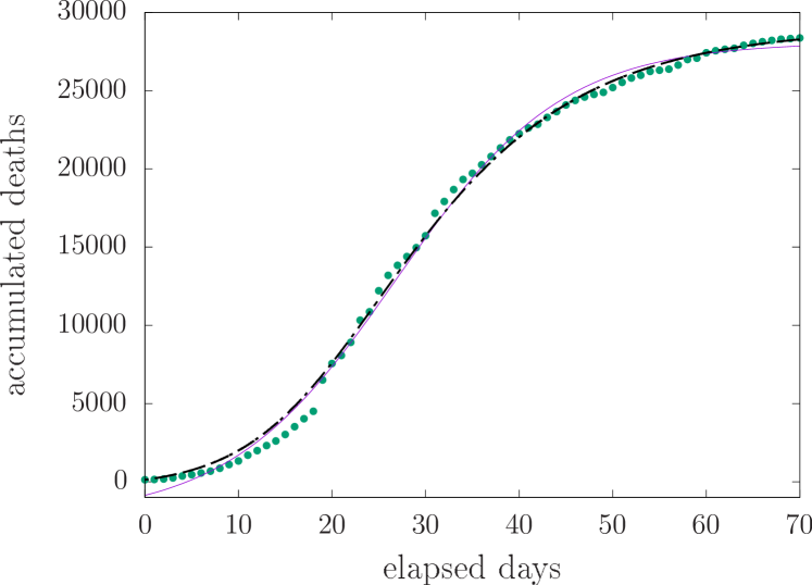
Figure 3: Issues when one tries to model the data with a single time window using French COVID-19 deaths from March 16 to May 25. Parameter optimization of the SIR model (dashed line) agrees well with input data (circles), especially after April 5. The optimization neglects the effects of control measures to reduce the transmission rate, while reducing the removal rate to $\lambda=0.103$ day^-1. The fit by a sigmoidal curve (solid line) underestimates $g_{\infty}$ and the curve turns negative in early March.

The observation above inquires whether the SIR model describes the data or not. However, this issue can be understood by inspecting the number of daily deaths (see Fig. 1a). An asymmetry is observed around the peak of daily deaths (see Fig. 1b), which is in sharp contrast with the corresponding curve in the theoretical SIR model (see Fig. 2b). The asymmetry can be explained by a variation in the transmission rate. Unlike other recent epidemics, several countries have adopted control measures such as lockdowns of non-essential workers, flight and other travel restrictions. The efforts effectively reduce the transmission rate of COVID-19 once they are in place. Thus, the data must be divided in non-overlapping time windows, each with its own set of epidemiological parameters.

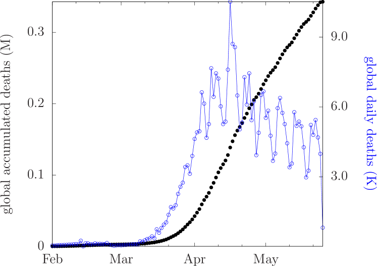
Figure 4: Global evolution of COVID-19. Accumulated deaths in millions (full circles). Daily deaths in the thousands (line with circles).

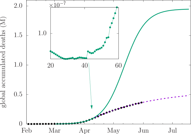
Figure 5: Time windows and the global evolution of COVID-19. The data (circles) are separated in two consecutive time windows (February 29 - April 9) and (April 10 - May 31). The fit (7) in the first time window (solid line) predicts over $2.0$ million deaths in a scenario without control measures. With control measures in place in the second time window, the death toll converges to $0.6$ million deaths (dashed line). (inset) residue per degree of freedom $r^{2}$. The size of the first time window is chosen as to maximize the adherence of the fitting curve (minimize $r^{2}$) while increasing the number of data points. $r^{2}$ forms a plateau for sizes between $29$ to $41$ days followed by a sudden increase for $42$ days, indicating that $41$ days is the optimal size of the time window (February 29 - April 9).

As a first example of data where the necessity to consider several time windows is obvious, we consider the global deaths between February 29 and May 31 (see Fig. 4). This case is interesting because countries afflicted by the epidemic have implemented various control measures at different schedules, of varying effectiveness. Thus, reduction of the global transmission rate cannot be pinpointed to a single day or week a priori. Similar to Fig. 1, the number of daily deaths exhibits an asymmetry, with center in mid-April, indicating the approximate interval in which the global transmission rate changes. European countries with most cases at the time (France, Italy, Spain) introduced lockdown and other strategies in mid-March, with others following shortly. Afterwards, the daily number of deaths starts to reduce, followed by an oscillatory pattern (7 days period) likely tied to work routines of medical staff and death cases reports.

In the following, we decide to divide the observation time in two consecutive time windows. Let us explain how we determine the optimal separation time (optimal duration of the first time window). Let $g_{k}$ be the fraction of the global population that dies due to complications caused by COVID-19, starting from February 29. The index $k=0,1,\ldots,m-1$ indicates the number of elapsed days in the time window with duration $m$. The data are fitted via (7) with parameters $g_{\infty},a,b$ and $\tau$, using trust region reflective algorithm (Python/Scipy). It is convenient to fit the data using $\tau^{-1}$ instead of $\tau$ and a finite interval $0\leqslant\tau^{-1}\leqslant 1$, so the infection lasts at least one day in the mathematical model. In the fitting procedure, we use bounds for $b$ which depends on the time interval $t_{c}$ between the inflection point and the initial entry, more specifically, $t_{c}=\tau\ln b$. For $t_{c}>0$ we restrict the search to $t_{c}/\tau<10$ so that $b\sim o(10^{4})$; for $t_{c}<0$, i.e., starting the counting after the inflection point, the parameter space of $b$ is limited between 0 and 1. Thus, we set the $0<b\leqslant 10^{4}$. The remaining parameters are restricted to $0\leqslant g_{\infty},a\leqslant 1$.

The quality of the fit is quantified by the square residue divided by the size of time window, namely, $r^{2}=(1/m)\sum_{k=0}^{m-1}[g_{k}-g_{\textrm{eff}}(k)]^{2}$. The first time window comprises $m$ consecutive days that minimize $r^{2}$ while increasing $m$, as indicated by the inset in Fig. 5, from February 29 to April 10, whereas days starting from the $m+1$ day are put into the second time window. The curve fit in the first interval corresponds to a scenario in which control measures were not implemented outside China and South Korea. These two time windows are consistent with the asymmetry observed in the number of daily deaths in Fig. 4, whose peak lies in mid-April. The fit converges to near $2.0$ million deaths, significantly above the equilibrium value ($0.6$ million deaths) in the second time window, from April 11 to May 31. We stress that the number of fatalities avoided ($1.4$ million) highlights the effectiveness of lockdowns and other control measures.

The curve fitting in the first time window, which includes the phase with exponential growth, can be challenging though. Even more so if the fitting data contains a large number of entries around the inflection point induced by the introduction of control measures. This inflection point is not the natural inflection point which occurs in an uncontrolled epidemic with constant parameters. Due to the significance of inflection points in the curve fitting, the induced inflection point can be responsible for the artificially low value of the equilibrium value $g_{\infty}$ in the first time window. Also, early data often contain far less entries, thus being more susceptible to fluctuations.

Conversely, the presence of inflection points caused by the introduction of control measures greatly simplifies the fitting procedure in the second time window. For instance, Fig. 6 depicts the death toll in Denmark after April 3, within the second time window. The fitting (7) is in excellent agreement with data for $g_{\infty}=(1.03\pm 0.01)\times 10^{-4}$ (approximately $600$ deaths) and $\tau=15.84\pm 0.65$ days. Next, we solve the system (8a-8c) for $\lambda$ distributed according to some probability distribution, centered around $\lambda=0.2$ days^-1. In practical terms, the width of the probability distribution forms the ground to compute uncertainties of the transmission and crude mortality rates. However, the finer details of the distribution of $\lambda$ remain unknown so we resort to a uniform distribution for virus shedding, whose interval lies between 3 and 7 days [25, 20]. By doing so, we overestimate the uncertainties of the remaining epidemiological parameters of the SIR model and find $\mathcal{R}_{0}=0.81\pm 0.07$. Our estimate for the crude mortality rate $f=(0.68\pm 0.15)\times 10^{-4}$ is compatible with the estimate $f_{\textrm{DNK}}=8.2\times 10^{-4}$ ( confidence interval: $[5.9-15.4]\times 10^{-4}$) obtained by screening antibodies of $20640$ blood donors below the age of 70, in Denmark [26]. Also, the asymptotic value $R_{\infty}=g_{\infty}/f=0.15\pm 0.03$ places the fraction of infected well below the threshold ($60\%$) for herd immunity. Thus, a new wave of infections is likely to occur if the disease becomes seasonal unless a vaccine becomes available or social distancing measures remain in place.

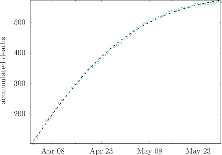
Figure 6: COVID-19 deaths in Denmark from April 4 to May 31. The sigmoidal fitting (line) of input data (cicles) followed by the resolution of (8a-8b) produce $\mathcal{R}_{0}=0.81$ and $f=6.86\times 10^{-4}$.

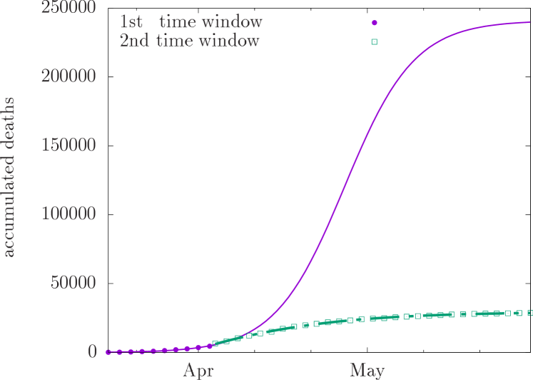
Figure 7: Evolution of COVID-19 in France between March 16 and May 31. Reduced number of data points for clarity. Data (full circles) and sigmoidal fit (solid line) between March 16 and April 3, with $\mathcal{R}_{0,1}=3.25$ and crude mortality rate $f_{1}=4.23\times 10^{-3}$. The effects of confinement emerge shortly after April 3, with a significant reduction in $\mathcal{R}_{0,2}=0.74$, as indicated by the sigmoidal fit (dashed line) of data in the second time window (empty squares). The mortality rate remains nearly unchanged $f_{2}=4.60\times 10^{-3}$.

We can now move to more complicated cases, in which the data themselves contains artifacts and the fitting procedure can be tricky. That is the case of France, for instance. The lockdown was issued on March 16, and unaccounted deaths in nursing homes were added to the official statistics on April 3 and 4, producing a large fluctuation in the number of daily deaths. In this case, we separate the time windows according to the number of deaths. The first time window lies between 100 and 5000 deaths (March 16 - April 3), whereas the remaining days until May 31 comprises the second time window, as shown in Fig. 7.

The curve fitting in the second time window is far more stable and insensitive to initial guesses, or bounds, with equilibrium death toll nearing $29440\pm 158$ and time scale $\tau=15.12\pm 0.72$ days, which approaches the typical recovery time for mild COVID-19 infections. The solution of the system (8a-8c) returns $\mathcal{R}_{0,2}=0.74\pm 0.08<1$ in agreement with the decline of new infections, where the notation $\mathcal{R}_{0,k}$ with $k=1$ and $2$ refers to the first and second time windows, respectively. In addition, the crude mortality rate in the second time window reads $f_{2}=(4.67\pm 1.16)\times 10^{-3}$, one order of magnitude higher than Denmark or Germany (see Table. 2).

Table 2: Parameters of the SIR model and sigmoid from April 4 to May 31 for selected countries, using a uniform distribution for $\lambda$.

	$\alpha$	$\mathcal{R}_{0}$	$f\,(10^{-3})$	$S_{0}$	$g_{\infty}\,(10^{-4})$
France	$0.17\pm 0.07$	$0.74\pm 0.08$	$4.67\pm 1.16$	$0.97\pm 0.02$	$4.40\pm 0.02$
Italy	$0.19\pm 0.07$	$0.84\pm 0.07$	$4.17\pm 0.78$	$0.96\pm 0.02$	$5.75\pm 0.01$
Spain	$0.19\pm 0.07$	$0.83\pm 0.07$	$2.31\pm 0.63$	$0.90\pm 0.06$	$6.08\pm 0.04$
UK	$0.18\pm 0.07$	$0.82\pm 0.07$	$5.86\pm 1.08$	$0.97\pm 0.01$	$6.26\pm 0.05$
Germany	$0.18\pm 0.07$	$0.83\pm 0.07$	$0.39\pm 0.11$	$0.90\pm 0.06$	$1.05\pm 0.01$
Sweden	$0.19\pm 0.07$	$0.85\pm 0.06$	$4.84\pm 0.77$	$0.98\pm 0.01$	$5.08\pm 0.18$
Denmark	$0.18\pm 0.07$	$0.81\pm 0.07$	$0.68\pm 0.15$	$0.95\pm 0.02$	$1.03\pm 0.01$
Belgium	$0.17\pm 0.07$	$0.73\pm 0.08$	$9.97\pm 2.55$	$0.97\pm 0.02$	$8.54\pm 0.05$

The analysis in the first time window requires more care. The fitting procedure requires bounds, otherwise the fit may incorrectly converge to an equilibrium value that is much lower than the one obtained for the second time window. In addition, multiple solutions can be found for (8a-8c), several of which are not realistic. Instead of using brute force, it is far more convenient to approximate the solution and set $S_{0}=0.99$. In such case, (8c) is discarded and the remaining equations produce $\mathcal{R}_{0,1}=3.25\pm 1.71$. The crude mortality rate in the first time window, $f_{1}=(4.23\pm 0.58)\times 10^{-3}$, shares the same order of magnitude as $f_{2}$, indicating that overall the French health care system remained responsive throughout the epidemic. If control measures had not been implemented, the expected number of deaths would have soared and reached 240 000, with equilibrium infected fraction of population $R_{\infty}=0.96$, assuming the mortality rate would have remained roughly the same.

6 Conclusion

The tragic developments in the COVID-19 pandemic have exposed flawed aspects in protocols used to assess large scale epidemics. Despite the various improvements in the global capacity to produce laboratory tests, usually based on reverse-transcription polymerase chain reaction (rRT-PCR), the majority of afflicted countries were unable to enforce mass testing policies. This shortcoming has also been experienced in 2002 with the SARS epidemic but in a smaller scale. The lack of mass testing contributed in keeping the number of cases unknown, affecting the accuracy of disease spreading models. In this paper, we resort to the death toll from April 4 to May 31 instead of reported cases as our primary data source as death certificates are mandatory and may contain other medical assessments linking the cause of death with COVID-19 outbreaks. We emphasize this methodology is not immune itself from sub-notification, nor unforeseen delays on death certificates.

We model the death toll via the sigmoid curve in (7), which requires the parameters $g_{\infty}$ (capacity) and $\tau$ (time scale). The capacity limits the growth of the outbreak, which is expected to vary with geographic region, healthcare quality, and efforts to control the spreading of the virus. Together with the crude mortality rate $f$, which also depends on healthcare and population demographics, they give access to a far more credible estimate for the infected fraction of the population $R_{\infty}=g_{\infty}/f$. To keep the model as simple as possible, we also neglect temporal delays between $g(t)$ and $R(t)$. The inclusion of said delay may introduce additional effects, but those are not expected to be dominant in this case since spatial effects are not being investigated.

The advantage of our approach relies on the curve fitting of a monotonic curve (death toll) to a sigmoid in sharp contrast to complex optimization schemes for models with multiple health states [20, 21]. Epidemiological parameters are extracted by solving the algebraic system of equations (8a-8c) for transmission rate, crude mortality rate and initial condition, respectively, $\alpha,f,$ and $S_{0}$. Alternatively, the epidemiological parameters calculated from the curve fitting can be used as educated guesses in optimization algorithms reducing the likelihood of obtaining unrealistic optimal solutions. We stress that if $f$ is known, then the fraction of reported cases can be easily computed $R(t)=g(t)/f$. We find that $f$ ranges from $o(10^{-4})$ to $o(10^{-3})$, depending on geographic location. Such values lie well below recent the estimate [27] using only rRT-PCR tests from hospitalized cases ($7.2\%$), whereas it is more in line with the values obtained from antibody screening with large sample size in Denmark [26]. Interestingly, countries lightly afflicted by the epidemic exhibit lower $f$ even though the transmission of the virus is similar to neighbouring countries. Taking Germany or Denmark as examples, we see that both have $f\sim o(10^{-4})$ while maintaining $\mathcal{R}_{0}$ compatible with other European countries. The result is likely attributed to healthcare resources and services either being more accessible or efficient, including early surveillance.

The sigmoidal fitting becomes far more reliable once the outbreak has been active for some time as the data starts to move away from the exponential phase. The distance from the inflection point is another important factor that affects the quality of the fit, especially the value of $g_{\infty}$. The introduction of lockdowns and other social distancing measures reduce the transmission rate and effectively create a new inflection point, which is different from the one expected without control measures. Thus, the fitting curve may converge to an incorrect equilibrium value if the fitting data include points around the induced inflection point. This can only be solved by introducing disjoint time windows for different regimes of $\alpha$ as Fig. 7 shows. The difference between the equilibrium values of $g_{\infty}$ from each time window returns the fraction of avoided deaths and it evaluates the effectiveness of control measures and policies. For instance, approximately $210\,000$ deaths or about seven times the current projection have been avoided in France. This is compatible with the large decrease in the basic reproduction number, placing it below the endemic threshold. However, some care is needed in interpreting these estimates as our analysis considers only two time windows and therefore does not anticipates second waves of infections.

Concerning deviations in parameters estimated through (8a-8c), they can be tracked to the uncertainties in the removal rate. In general, the inverse of the removal rate describes the average time required for an infective person to change to the removed state. For COVID-19, virus shedding occurs more prominently between 3 and 7 days, with a peak at day 5 since the onset of symptoms [25]. The exact probability distribution for $\lambda$ remains an open issue so our analysis assume a uniform distribution.

Finally, the SIR model rests on the random mixing hypothesis but deviations are expected with stronger effects in population with varying demographics or populations at risk. In particular, communicable respiratory diseases become major issues in correctional facilities, given the lack of adequate environmental and sanitary conditions. The combination of higher transmission rate of pathogens and reduced removal rate with reduced healthcare can increase the crude mortality rate for incarcerated individuals. By a similar argument, outbreaks in nursing homes may affect estimates of epidemiological parameters because the disease becomes disproportionately more lethal for older patients. In this study, both effects are neglected in hopes to understand the disease spreading of the average population with the minimal number of parameters possible.

Author contributions statement

GN wrote the paper and carried out the numerical analysis. CD, BG, and MB designed the research and edited the paper. All authors reviewed the manuscript.

Data availability

The datasets analysed and numerical code generated during the current study are available in the Zenodo repository, https://doi.org/10.5281/zenodo.3931666

Additional information

Competing interests The authors declare no conflict of interest.

References

- [1] Morabia, A. A history of epidemiologic methods and concepts (Birkhauser Verlag, Basel Boston, 2004).
- [2] WHO. World Health Statistics 2018 : monitoring health for the SDGs : sustainable development goals (World Health Organization, Geneva, Switzerland, 2018).
- [3] Mlakar, J. et al. Zika virus associated with microcephaly. N. Engl. J. Med. 374, 951–958 (2016). URL http://dx.doi.org/10.1056/NEJMoa1600651. http://dx.doi.org/10.1056/NEJMoa1600651.
- [4] de Oliveira, W. K. et al. Infection-related microcephaly after the 2015 and 2016 zika virus outbreaks in Brazil: a surveillance-based analysis. Lancet 390, 861 – 870 (2017). URL http://www.sciencedirect.com/science/article/pii/S0140673617313685.
- [5] Team, W. E. R. West african ebola epidemic after one year — slowing but not yet under control. N. Engl. J. Med. 372, 584–587 (2015). URL http://dx.doi.org/10.1056/NEJMc1414992. http://dx.doi.org/10.1056/NEJMc1414992.
- [6] Van Kerkhove, M. D., Bento, A. I., Mills, H. L., Ferguson, N. M. & Donnelly, C. A. A review of epidemiological parameters from ebola outbreaks to inform early public health decision-making. Sci. Data 2, 150019 EP – (2015). URL http://dx.doi.org/10.1038/sdata.2015.19. Data Descriptor.
- [7] Simonsen, L. et al. Global mortality estimates for the 2009 influenza pandemic from the glamor project: A modeling study. PLOS Med. 10, 1–17 (2013). URL https://doi.org/10.1371/journal.pmed.1001558.
- [8] Chan, J. F.-W. et al. A familial cluster of pneumonia associated with the 2019 novel coronavirus indicating person-to-person transmission: a study of a family cluster. Lancet 395, 514–523 (2020). URL https://doi.org/10.1016/S0140-6736(20)30154-9.
- [9] Chen, N. et al. Epidemiological and clinical characteristics of 99 cases of 2019 novel coronavirus pneumonia in Wuhan, China: a descriptive study. Lancet 395, 507–513 (2020). URL https://doi.org/10.1016/S0140-6736(20)30211-7.
- [10] WHO. Report of the WHO-China joint mission on coronavirus disease 2019 (covid-19) (2020). Access April 20, 2020.
- [11] Baud, D. et al. Real estimates of mortality following COVID-19 infection. Lancet Infect. Dis. (2020). URL https://doi.org/10.1016/S1473-3099(20)30195-X.
- [12] Walker, P. et al. Report 12: The global impact of COVID-19 and strategies for mitigation and suppression. Tech. Rep., Imperial College London (2020). URL http://doi.org/10.25561/77735.
- [13] Keeling, M. & Eames, K. Networks and epidemic models. J. R. Soc. Interface 2, 295–307 (2005).
- [14] Bansal, S., Grenfell, B. T. & Meyers, L. A. When individual behaviour matters: homogeneous and network models in epidemiology. J. R. Soc. Interface 4, 879–891 (2007).
- [15] Kucharski, A. J. et al. Early dynamics of transmission and control of COVID-19: a mathematical modelling study. Lancet Infect. Dis. 20, 553–558 (2020). URL https://doi.org/10.1016/S1473-3099(20)30144-4.
- [16] Li, Q. et al. Early transmission dynamics in Wuhan, China, of novel coronavirus–infected pneumonia. N. Engl. J. Med. 382, 1199–1207 (2020). URL https://doi.org/10.1056/nejmoa2001316.
- [17] Sanche, S. et al. High contagiousness and rapid spread of severe acute respiratory syndrome coronavirus 2. Emerg. Infect. Dis. 26 (2020). URL https://doi.org/10.3201/eid2607.200282.
- [18] Kermack, W. O. & McKendrick, A. G. A contribution to the mathematical theory of epidemics. Proc. R. Soc. A 115, 700–721 (1927). URL http://rspa.royalsocietypublishing.org/content/115/772/700.
- [19] European-Center of Disease Prevention and Control. & Geographic distribution of COVID-19 cases worldwide (2020). Dataset retrieved from https://opendata.ecdc.europa.eu/covid19/casedistribution/csv.
- [20] Prem, K. et al. The effect of control strategies to reduce social mixing on outcomes of the COVID-19 epidemic in Wuhan, China: a modelling study. Lancet Public Health (2020). URL https://doi.org/10.1016/S2468-2667(20)30073-6.
- [21] Giordano, G. et al. Modelling the COVID-19 epidemic and implementation of population-wide interventions in Italy. Nat. Med. (2020). URL https://doi.org/10.1038/s41591-020-0883-7.
- [22] Gandhi, R. T., Lynch, J. B. & del Rio, C. Mild or moderate covid-19. N. Engl. J. Med. (2020). URL https://doi.org/10.1056/nejmcp2009249.
- [23] Ota, M. Will we see protection or reinfection in COVID-19? Nat. Rev. Immunol. (2020). URL https://doi.org/10.1038/s41577-020-0316-3.
- [24] Harko, T., Lobo, F. S. & Mak, M. Exact analytical solutions of the susceptible-infected-recovered (sir) epidemic model and of the sir model with equal death and birth rates. Appl. Math. Comput. 236, 184 – 194 (2014). URL http://www.sciencedirect.com/science/article/pii/S009630031400383X.
- [25] Wölfel, R. et al. Virological assessment of hospitalized patients with COVID-2019. Nature 581, 465–469 (2020). URL https://doi.org/10.1038/s41586-020-2196-x.
- [26] Erikstrup, C. et al. Estimation of SARS-CoV-2 infection fatality rate by real-time antibody screening of blood donors. Clin. Infect. Dis. (2020). URL https://doi.org/10.1093/cid/ciaa849.
- [27] Onder, G., Rezza, G. & Brusaferro, S. Case-fatality rate and characteristics of patients dying in relation to COVID-19 in Italy. JAMA (2020). URL https://doi.org/10.1001/jama.2020.4683.